Rotation-Angle Solution and Singularity Handling of Five-Axis Machine Tools for Dual NURBS Interpolation

Abstract

Dual NURBS interpolation has been proven an essential technique for high-speed precision machining of complex surfaces. The solution of rotation angles and their derivatives is the basis of kinematic transformation and feedrate optimization in dual NURBS interpolation. The characteristics of the rotation motion of five-axis machine tools with different structures are analyzed. A generic model of dual heads of the vertical five-axis machine tool is established to unify the solution of rotation angles. Then, a generic method for solving the rotation angles and derivatives based on the vector inner product is proposed, and the solution space is analyzed. A singularity handling is given to avoid abrupt rotation angles based on the higher derivatives of the tool orientation vector. The proposed method obtained smooth rotation angles at the singularity points in the cardioid dual NURBS interpolation experiment. It reduced the machining time by 43.3% compared with the simple inverse trigonometric method based on kinematic transformation. Experiment results demonstrate that the proposed method is feasible and effective, and has significant theoretical and practical value for optimizing five-axis CNC machining.

1. Introduction

With the application of complex surface structural parts in aerospace, automobile, shipbuilding, energy, and power industries, five-axis CNC machining has become an essential method of high-efficiency and quality machining of complex surface parts. As one of the critical technologies of five-axis NC machining, kinematic transformation is to determine the relationship between the tool path and the feeding axis according to the structural form and parameters of the machine tool. At the same time, to realize high-order continuous smoothing of the machining trajectory and further improve the machining accuracy and efficiency, the direct interpolation of dual NURBS curves has become the focus research topic in five-axis machining [1,2]. The tool orientation vector is changed from the original discrete vector to a high-order continuous vector in the representation of the tool path using dual NURBS curves. The CNC system needs to calculate the rotation angles corresponding to the tool orientation vector and the derivatives of the rotation angles with respect to the curve parameter, which becomes the difficulty and emphasis in five-axis kinematic transformation [3]. Therefore, it is of great significance to study five-axis linkage kinematic models with different structural forms and to realize the method of solving the rotation angles for direct interpolation of dual NURBS curves.

The solution of the rotation angles of a five-axis machine tool is generally a part of the solution of the five-axis inverse kinematics. For five-axis CNC machine tools with different structural forms, kinematic solving methods mainly include the following three types: (1) a model based on mechanism and homogeneous coordinate transformation [4,5,6,7,8,9]; (2) a generic model based on multi-body kinematics theory [10,11]; (3) a general kinematic solution method based on a decoupling and differential method [12,13,14]. Although the above methods can realize the solution of the rotation angles, they may lead to an abrupt rotation angle at the singular point [15,16]. Scholars have also researched the smoothing of the rotation axis and the optimization of singular points of five-axis machine tools. Farouki, R.T. et al. [17] studied the inverse kinematic solution problem to minimize the orientation change between the tool axis and the surface normal under the constraint of constant cutting speed, while the solution is dependent upon the surface normal along the toolpath. Lin, T.K. et al. [18] proposed a general method to convert the tool position (CL) data into NC data for the non-orthogonal worktable type five-axis machine tool. The rotation angles of two rotation axes can be directly derived from the tool orientation vector. Yu, D. et al. [19] proposed a method of integrating corner selection, optimization, and singular region processing to solve the problems of the collision. Although this method is effective in solving the problems of rotation-angle optimization of linear segments and singularity processing, it cannot be used in curve direct interpolation. Hong, X.Y. et al. [20] proposed a singularity optimization method based on the rotation change rate which adjusts the tool orientation vector by controlling the rotation change rate to avoid the singular problem in five-axis machining. Beudaert, X. et al. [21] proposed a decoupling method for separating the geometric processing of the programmed tool path from the feedrate interpolation, and the algorithm is complicated to calculate. Through the iterative algorithm, the motion parameters of each axis are solved. In addition, scholars also realized smoothing by adjusting the discrete tool direction change of the tool path [22]. Li, Z. [11] improved the calculation method of the rotation angle by defining the “minimum movement circle” to improve the rotation continuity of the C-axis workbench effectively, and the method is limited to the five-axis orthogonal machine tools with a C turntable. Castagnetti, C. et al. [23] confirmed that the kinematic performance of five-axis machining can be improved by sliding the rotation axes in the machine coordinate system rather than adjusting the tool orientation in the workpiece coordinate system. Wang, Q.R. et al. [24] constructed a discrete domain of feasible directions at the tool path points and optimized the tool direction sequence with the shortest path, bypassing the singularity by changing the tool directions. Hu, P.C. et al. [25] established the angular acceleration function according to the numerical solution of the inverse kinematic equations, which realized the directional constraint optimization of the tool axis.

It is the standard method to establish the relationship between the tool orientation and the rotation angles according to the homogeneous transformation and calculate the rotation angles by the inverse trigonometric function [26]. Calculating the rotation transformation matrix of the non-orthogonal rotation axes is more complex. The main problems are as follows: (1) the range of arcsine and arccosine functions is often limited to the semicircle angle, which cannot make full use of the stroke of the rotation axes; (2) there may be infinite solutions at the singular point of the tool orientation, which results in violent and uncontrollable movements of machine tools.

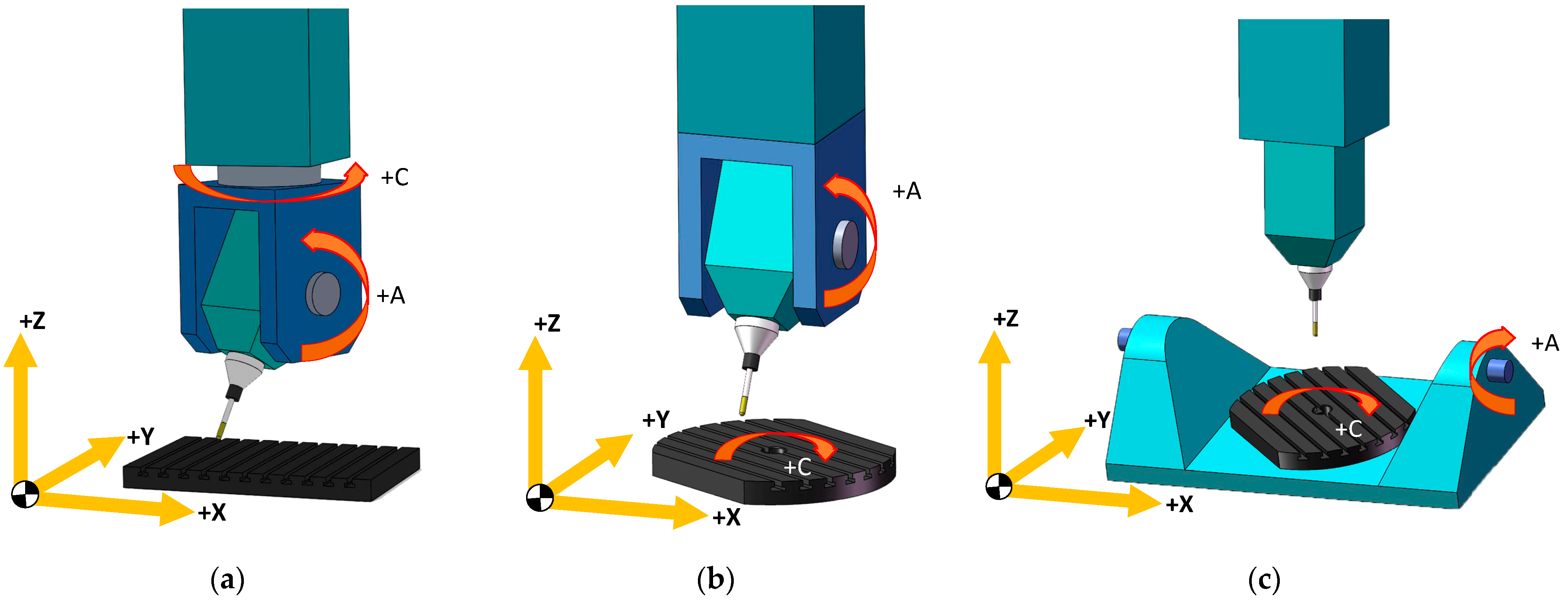
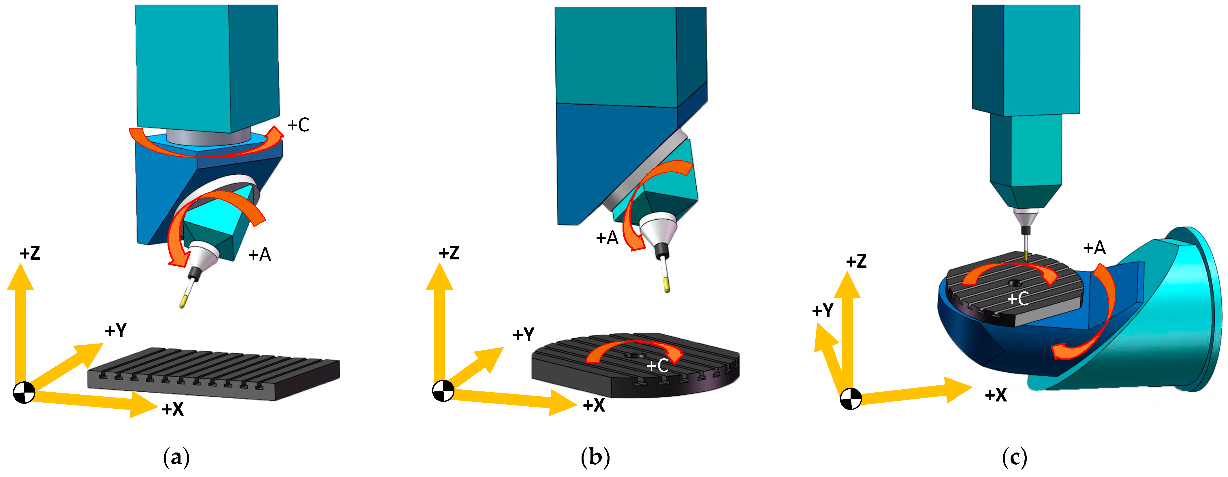
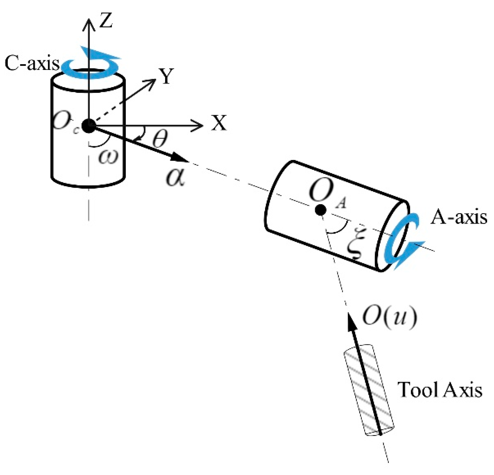
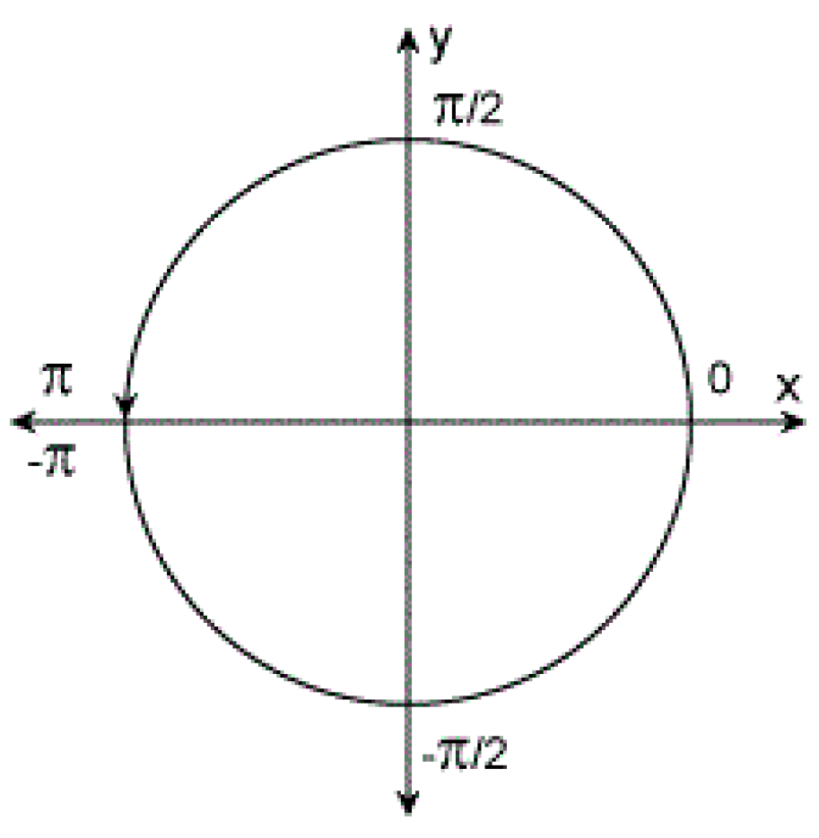
To solve the above problems, this paper focuses on the generic solution of the rotation angles of five-axis machine tools for dual NURBS direct interpolation, and a singularity handling method is given. The organization of the rest of this paper is as follows: In chapter 2, the direct interpolation model of dual NURBS curves is given, and rotation motion characteristics of the typical dual rotation axes layout are studied. The generic method for solving the rotation angles of five-axis machine tools based on the vector inner product is proposed, and the rotation-angle solution space and singularity handling are analyzed. In chapter 3, the effectiveness and superiority of the method are verified and compared. In chapter 4, the research contents and experimental results are summarized.

2. Rotation-Angle Solution of Five-Axis Machine Tools for Dual NURBS Interpolation

2.1. Dual NURBS Interpolation

Dual NURBS generally consists of the tool tip point trajectory curve and the scanning curve of the tool axis point, shown as follows:

$$\{\begin{array}{l}C\left(u\right)=\frac{{\displaystyle \sum _{i=0}^n{N}_{i,p}\left(u\right)w_i{P}_i}}{{\displaystyle \sum _{i=0}^n{N}_{i,p}\left(u\right)w_i}}\\ T\left(u\right)=\frac{{\displaystyle \sum _{i=0}^n{N}_{i,p}\left(u\right)w_i{H}_i}}{{\displaystyle \sum _{i=0}^n{N}_{i,p}\left(u\right)w_i}}\end{array}$$

(1)

where $C\left(u\right)$ is the trajectory curve of the tool tip point, $T\left(u\right)$ is the scanning trajectory curve of a fixed point on the tool axis, $\left\{P_i|i=0,1,\dots ,n\right\}$ are the control points of the curve $C\left(u\right)$, $\left\{H_i|i=0,1,\dots ,n\right\}$ are the control points of the curve $T\left(u\right)$, $\left\{w_i|i=0,1,\dots ,n\right\}$ are the factors, and $N_{i,p}\left(u\right)$ is the pth-degree B-spline basis function defined on the quasi-uniform knot vector $U=\left[u_0,u_1,\dots ,u_{n+p},u_{n+p+1}\right]$.

The B-spline basis function can be calculated as follows:

$$\{\begin{array}{l}{N}_{i,p}\left(u\right)=\frac{u-u_i}{u_{i+p}-u_i}{N}_{i,p-1}\left(u\right)+\frac{u_{i+p+1}-u}{u_{i+p+1}-u_{i+1}}{N}_{i+1,p-1}\left(u\right)\\ N_{i,0}\left(u\right)=\{\begin{array}{l}1,u_i\le u\le u_{i+1}\\ 0, \mathrm{otherwise}\end{array}\end{array}$$

(2)

The vector of the tool orientation $O\left(u\right)$ is expressed as:

$$O\left(u\right)=\frac{T\left(u\right)-C\left(u\right)}{\Vert T\left(u\right)-C\left(u\right)\Vert }$$

(3)

The interpolation process of dual NURBS is to calculate the following parameter of the spline in each cycle task that satisfies the distance between the current point and the next point of the curve equal to the step length.

$$\Vert C\left(u_{i+1}\right)-C\left(u_i\right)\Vert =\Delta s_i$$

(4)

where $u_i$ is the current curve parameter, $u_{i+1}$ is the next curve parameter, and $\Delta s_i$ is the current step length, which can be determined by the velocity and acceleration in the interpolation interval.

The parameter $u_{i+1}$ can be estimated by Taylor series expansion.

$$u_{i+1}=u_i+u_s\left(u_i\right)\Delta s_i+\frac{1}{2}{u}_{ss}\left(u_i\right){\left(\Delta s_i\right)}^2$$

(5)

where $u_s\left(u_i\right)$ is the current derivative of the parameter with respect to the arc length of curve $C\left(u\right)$, and $u_{ss}\left(u_i\right)$ is the current second derivative of the parameter with respect to the arc length.

The linear feed-axis positions are obtained by the kinematic transformation of the machine tool, and the homogeneous form of the transformation can be expressed as follows:

$$\left[\begin{array}{c}{Q}_{L,i+1}\\ 1\end{array}\right]=\mathbf{M}\left({\theta }_{i+1},{\phi }_{i+1}\right)\left[\begin{array}{c}C\left(u_{i+1}\right)\\ 1\end{array}\right]$$

(6)

where $Q_{L,i+1}$ is the position vector of linear axes, $C\left(u_{i+1}\right)$ is the interpolation tool tip location in the workpiece coordinate system, $\mathbf{M}\left({\theta }_{i+1},{\phi }_{i+1}\right)$ is the homogeneous matrix of the kinematic transformation from workpiece coordinate system to machine tool coordinate system, and ${\theta }_{i+1}$ and ${\phi }_{i+1}$ are the current rotation angles of the machine tool under the current tool orientation vector $O\left(u_{i+1}\right)$. The matrix $\mathbf{M}\left(\theta ,\phi \right)$ is a nonlinear matrix function of the rotation angles $\theta$ and $\phi$, which can be obtained according to the kinematic chain of the machine tool by the Denavit–Hartenberg transformation method.

The feedrate of the dual NURBS is usually optimized offline based on optimization theory to achieve the minimum interpolation time under geometric, kinematic, and dynamic constraints. The constraints of feed axes can be expressed as follows:

$$\{\begin{array}{l}\left|\dot{q}\left(u\right)\right|=\left|q_s\left(u\right)V\left(u\right)\right|\le V_{m,q}\\ \left|\ddot{q}\left(u\right)\right|=\left|q_{ss}\left(u\right)V{\left(u\right)}^2+q_s\left(u\right)A\left(u\right)\right|\le A_{m,q}\\ \left|\stackrel{⃛}{q}\left(u\right)\right|=\left|q_{sss}\left(u\right)V{\left(u\right)}^3+3q_{ss}\left(u\right)V\left(u\right)A\left(u\right)+q_s\left(u\right)J\left(u\right)\right|\le J_{m,q}\end{array}q=X,Y,Z,\cdots$$

(7)

where q represents a specific axis position of the machine tool, $\dot{q}\left(u\right),\ddot{q}\left(u\right),\stackrel{⃛}{q}\left(u\right)$ are, respectively, the velocity, acceleration, and jerk of the machine tool feed axis q corresponding to the curve parameter u, $q_s,q_{ss},q_{sss}$ are, respectively, the first, second, and third derivatives of the feed-axis position with respect to the curve arc parameter, which can be calculated by taking high-order derivatives of Equation (6). $V\left(u\right)$ is the feedrate of the dual NURBS interpolation, $A\left(u\right)$ is the tangential acceleration, $J\left(u\right)$ is the tangential jerk, and $V_{m,q},A_{m,q},J_{m,q}$ are, respectively, the maximum allowable velocity, acceleration, and jerk of the machine tool feed axis.

The axis positions and the derivatives of the machine tool can be calculated by the tool tip curve $C\left(u\right)$ and tool orientation vector $O\left(u\right)$ based on the kinematic transformation. Solving the corresponding rotation angle and derivatives according to the tool orientation vector is the basis of the dual NURBS interpolation and feedrate optimization.

2.2. Generic Method of Rotation-Angle Solution of Five-Axis Machine Tools

2.2.1. Typical Layouts of Rotary Axes of Five-Axis Machine Tools and Analysis

The layout of the dual-rotation axis of the five-axis machine tool can be divided into two categories: orthogonal structure and pendulous structure. In this paper, machine tools with AC rotation axes are taken as examples to describe the two structures, as shown in Figure 1 and Figure 2. For the machine tool with an orthogonal structure, the A-axis and C-axis rotation axes are perpendicular to the coordinate planes. Meanwhile, the tool axis and A-axis rotation axis are perpendicular. In contrast, for pendulous structure machine tools, only the C-axis rotation axis is perpendicular to the coordinate plane, while the A-axis rotation axis is usually perpendicular to neither the coordinate plane nor the tool axis.

According to the installation structure, the layouts of the machine tool with double rotation axes can be divided into three types: dual-head type, single-head and single-turntable type, and dual-turntable type.

For AC dual-turntable machine tools, the tool orientation vector rotates around axis X relative to the workpiece when the turntable rotates around A-axis, as shown in Figure 1c. For single-head and single-turntable machine tools, the A-axis rotation can also realize that the tool orientation vector rotates around axis X relative to the workpiece, as shown in Figure 1b. In the same way, the rotation motion of the orthogonal dual-head machine tool has the same effect on changing the relative tool orientation vector, as shown in Figure 1a.

Therefore, the rotation-angle solution of the dual-head type can represent the relationship between the rotation angles of the three orthogonal structure types and the tool orientation vector relative to the workpiece.

By the exact analysis of the rotation motion of the machine tools with pendulous rotary axes, as shown in Figure 2, the dual-head type can be used to unify the rotation angles solution of different types. Moreover, the tool orientation vector of the dual-head type is the same as that of the workpiece coordinate system, simplifying the solution process. In the following sections, the dual-head type machine tools will be taken as the specific research object.

2.2.2. Generic Method for Solving the Rotation Angles of Five-Axis Machine Tools Based on the Vector Inner Product

A generic dual-head model of the vertical five-axis machine tool is constructed, as shown in Figure 3. The C-axis rotation axis is parallel to the Z-axis. The angle between the A-axis rotation axis and the C-axis rotation axis is $\omega$, and the angle between the tool axis and the A-axis rotation axis is $\xi$. Due to the symmetry and requirements of five-axis machining, the angle ranges are $\omega \in (0,\pi ), \xi \in (0,\pi )$. The unit rotation axis direction vector of the A-axis can be expressed by the C-axis angle as follows.

$$\alpha ={\left[\sin \omega \cos \theta ,\sin \omega \sin \theta ,-\cos \omega \right]}^T$$

(8)

where $\alpha$ is the A-axis rotation axis vector, and $\theta$ is the rotation angle of the C-axis.

Since the angle between the tool orientation vector $O\left(u\right)$ and the unit rotation direction vector of the A-axis is a constant angle $\left(\pi -\xi \right)$, the inner product of the vector $O\left(u\right)$ and vector $\alpha$ is constant.

$$\mathrm{dot}\left(\alpha ,O\left(u\right)\right)=\cos \left(\pi -\varphi \right)=-\cos \xi$$

(9)

where dot( , ) is the inner-product function of vectors.

The equation of angle $\theta$ can be obtained as follows by substituting Equation (8) into Equation (9).

$$\sin \omega \left(i\cos \theta +j\sin \theta \right)=k\cos \omega -\cos \xi$$

(10)

where i, j, and k are the components of the vector $O\left(u\right)$ in the X-axis, Y-axis, and Z-axis.

As $\sin \omega >0$, Equation (10) can be reduced to the following equation:

$$i\cos \theta +j\sin \theta =\eta$$

(11)

where $\eta =\frac{1}{\sin \omega }\left(k\cos \omega -\cos \xi \right)$.

The solution of Equation (11) is calculated as follows, according to the knowledge of the conic curves when $i^2+j^2>{\eta }^2$.

$$\{\begin{array}{l}\cos \theta =\frac{\eta i+j\sqrt{i^2+j^2-{\eta }^2}}{i^2+j^2}\\ \sin \theta =\frac{\eta j-i\sqrt{i^2+j^2-{\eta }^2}}{i^2+j^2}\end{array},or\{\begin{array}{l}\cos \theta =\frac{\eta i-j\sqrt{i^2+j^2-{\eta }^2}}{i^2+j^2}\\ \sin \theta =\frac{\eta j+i\sqrt{i^2+j^2-{\eta }^2}}{i^2+j^2}\end{array}$$

(12)

The function $\arctan 2\left(Y,X\right)$ is a four-quadrant arctangent function, as shown in the Figure 4, and returns the angle value in the interval $\left[-\pi ,\pi \right]$ based on the values of Y and X.

The result of angle $\theta$ is solved as follows. The value closest to the previous angle of the C-axis is taken as the optimal solution to maintain the continuity of the angle of C-axis.

$$\{\begin{array}{l}{\theta }_1=\arctan 2\left(\eta j-i\sqrt{i^2+j^2-{\eta }^2},\eta i+j\sqrt{i^2+j^2-{\eta }^2}\right)\\ {\theta }_2=\arctan 2\left(\eta j+i\sqrt{i^2+j^2-{\eta }^2},\eta i-j\sqrt{i^2+j^2-{\eta }^2}\right)\end{array}$$

(13)

The derivative relation between vector O and $\alpha$ is obtained by differentiating the parameter u on both sides of Equation (9).

$$\{\begin{array}{l}\mathrm{dot}\left({\alpha }_u,O\right)+\mathrm{dot}\left(\alpha ,O_u\right)=0\\ \mathrm{dot}\left({\alpha }_{uu},O\right)+2\mathrm{dot}\left({\alpha }_u,O_u\right)+\mathrm{dot}\left(\alpha ,O_{uu}\right)=0\\ \mathrm{dot}\left({\alpha }_{uuu},O\right)+3\mathrm{dot}\left({\alpha }_{uu},O_u\right)+3\mathrm{dot}\left({\alpha }_u,O_{uu}\right)+\mathrm{dot}\left(\alpha ,O_{uuu}\right)=0\end{array}$$

(14)

Then, the higher derivatives of the angle $\theta$ with respect to the parameter u can be calculated as follows.

$$\{\begin{array}{l}{\theta }_u=\frac{-\mathrm{dot}\left(\alpha ,O_u\right)}{\mathrm{dot}\left({\alpha }_{\theta },O\right)}\\ {\theta }_{uu}=-\frac{\mathrm{dot}\left({\alpha }_{\theta \theta },O\right){\theta }_u^2+2\mathrm{dot}\left({\alpha }_u,O_u\right)+\mathrm{dot}\left(\alpha ,O_{uu}\right)}{\mathrm{dot}\left({\alpha }_{\theta },O\right)}\\ {\theta }_{uuu}=-\frac{\mathrm{dot}\left({\theta }_u^3{\alpha }_{\theta \theta \theta }+3{\theta }_u{\theta }_{uu}{\alpha }_{\theta \theta },O\right)+3\mathrm{dot}\left({\alpha }_{uu},O_u\right)+3\mathrm{dot}\left({\alpha }_u,O_{uu}\right)+\mathrm{dot}\left(\alpha ,O_{uuu}\right)}{\mathrm{dot}\left({\alpha }_{\theta },O\right)}\end{array}$$

(15)

The new tool orientation vector $\widehat{O}$ can be obtained as follows when both the tool axis and A-axis are rotated by angle $-\theta$ around the C-axis rotation axis.

$$\widehat{O}=\mathbf{Q}\cdot O\left(u\right)$$

(16)

where Q is the transformation matrix of the rotation around the C-axis. It can be expressed as follows.

$$\mathbf{Q}=\left[\begin{array}{ccc}\cos \theta & \sin \theta & 0\\ -\sin \theta & \cos \theta & 0\\ 0& 0& 1\end{array}\right]$$

(17)

The higher derivatives of the new tool orientation vector $\widehat{O}$ can be calculated as follows.

$$\{\begin{array}{l}{\widehat{O}}_u={\mathbf{Q}}_u\cdot O\left(u\right)+\mathbf{Q}\cdot O_u\left(u\right)\\ {\widehat{O}}_{uu}={\mathbf{Q}}_{uu}\cdot O\left(u\right)+2{\mathbf{Q}}_u\cdot O_u\left(u\right)+\mathbf{Q}\cdot O_{uu}\left(u\right)\\ {\widehat{O}}_{uuu}={\mathbf{Q}}_{uuu}\cdot O\left(u\right)+3{\mathbf{Q}}_{uu}\cdot O_u\left(u\right)+3{\mathbf{Q}}_u\cdot O_{uu}\left(u\right)+\mathbf{Q}\cdot O_{uuu}\left(u\right)\end{array}$$

(18)

The tool orientation vector $\widehat{O}$ can be expressed as follows by the A-axis angle $\phi$.

$$\widehat{O}=\left[\begin{array}{c}-\sin \omega \cos \xi +\cos \omega \sin \xi \cos \phi \\ -\sin \xi \sin \phi \\ \cos \omega \cos \xi +\sin \omega \sin \xi \cos \phi \end{array}\right]$$

(19)

The A-axis angle $\phi$ is solved by combining Equations (16) and (19).

$$\phi =\arctan 2\left(-\widehat{j},\widehat{i}\cos \omega +\widehat{k}\sin \omega \right)$$

(20)

where $\widehat{i}$, $\widehat{j}$, and $\widehat{k}$ are the components of the vector $\widehat{O}$ in the X-axis, Y-axis, and Z-axis.

The higher derivatives of the angle $\phi$ with respect to the parameter u can be calculated as follows.

$$\{\begin{array}{l}{\phi }_u=\frac{1}{{\sin }^2\xi }dot\left({\widehat{O}}_u,{\widehat{O}}_{\phi }\right)\\ {\phi }_{uu}=\frac{1}{{\sin }^2\xi }dot\left({\widehat{O}}_{uu}-{\widehat{O}}_{\phi \phi }{\theta }_u^2,{\widehat{O}}_{\phi }\right)\\ {\phi }_{uuu}=\frac{1}{{\sin }^2\xi }dot\left({\widehat{O}}_{uuu}-{\widehat{O}}_{\phi \phi \phi }{\theta }_u^3-3{\widehat{O}}_{\phi \phi }{\theta }_u{\theta }_{uu},{\widehat{O}}_{\phi }\right)\end{array}$$

(21)

2.3. Solution Space of the Generic Method

The A-axis angle exists and is unique after determining the C-axis angle according to Equation (20). Therefore, the solution space of rotation angles in the dual NURBS interpolation can be analyzed according to the solution of the C-axis angle. The solution space of the C-axis angle can be divided into three categories based on Equations (12) and (13).

(a)

No solution. The tool orientation vector $O\left(u\right)$ cannot be realized by rotation axes as the tool orientation vector is beyond the reach of the machine tool when $i^2+j^2<{\eta }^2$.

(b)

Finite solutions. The C-axis angle has two sets of solutions when $i^2+j^2\ge {\eta }^2$ and $i^2+j^2>0$, as shown in Equation (13). The rotation angles are high-order continuous with respect to the parameter u, when the tool orientation vector is high-order continuous.

(c)

Infinite solutions. The C-axis angle has infinite sets of solutions when $i^2+j^2={\eta }^2=0$. The tool orientation vector is at the singularity point, which cannot be changed no matter the C-axis angle. The tool orientation and the layout of rotation axes must meet the following conditions.

$$\{\begin{array}{l}O={\left[0,0,1\right]}^T\\ \omega =\xi \end{array} , \mathrm{or} \{\begin{array}{l}O={\left[0,0,-1\right]}^T\\ \omega +\xi =\pi \end{array}$$

(22)

The A-axis angle is always as follows at the singularity point.

$$\phi =\{\begin{array}{l}0, \mathrm{when} \omega =\xi \\ \pi , \mathrm{when} \omega +\xi =\pi \end{array}$$

(23)

2.4. Singularity Handling

The tool axis is parallel to the rotation axis of the C-axis when the tool orientation vector is located at the singularity point. The inner product of the tool orientation vector and any order derivative of the rotation axis vector of the A-axis is 0. Equation (14) can be simplified as follows.

$$\mathrm{dot}\left(\alpha ,O_u\right)=0$$

(24)

Since the modulus of the tool orientation vector is a constant of value 1, the first-order derivative vector $O_u={\left[i_u,j_u,k_u\right]}^T$ is perpendicular to the rotation axis of the C axis, and the value of $k_u$ is 0. Equation (24) can be expressed as follows.

$$\sin \omega \left(i_u\cos \theta +j_u\sin \theta \right)=0$$

(25)

The angle $\theta$ can be solved when $i_u^2+j_u^2>0$, while the equation needs more information such as the second derivative of vector $O\left(u\right)$ to be solved when $i_u^2+j_u^2=0$. The equation of $\theta$ can be established by higher derivates when the lower derivative information cannot determine the rotation angle. The handling is listed in

Table 1. Rotation-angle handling at the singularity point based on the derivatives of the tool orientation vector.

Conditions of the Tool Orientation	Equation of the Rotation Angle	Solutions
$\{\begin{array}{l}{i}^2+j^2=0\\ i_u^2+j_u^2>0\end{array}$	$\sin \omega \left(i_u\cos \theta +j_u\sin \theta \right)=0$	$\{\begin{array}{l}{\theta }_1=\arctan 2\left(-i_u,j_u\right)\\ {\theta }_2=\arctan 2\left(i_u,-j_u\right)\end{array}$
$\{\begin{array}{c}{i}^2+j^2=0\\ i_u^2+j_u^2=0\\ i_{uu}^2+j_{uu}^2>0\end{array}$	$\sin \omega \left(i_{uu}\cos \theta +j_{uu}\sin \theta \right)=0$	$\{\begin{array}{l}{\theta }_1=\arctan 2\left(-i_{uu},j_{uu}\right)\\ {\theta }_2=\arctan 2\left(i_{uu},-j_{uu}\right)\end{array}$
$\{\begin{array}{c}{i}^2+j^2=0\\ i_u^2+j_u^2=0\\ i_{uu}^2+j_{uu}^2=0\\ i_{uuu}^2+j_{uuu}^2>0\end{array}$	$\sin \omega \left(i_{uu}\cos \theta +j_{uu}\sin \theta \right)=0$	$\{\begin{array}{l}{\theta }_1=\arctan 2\left(-i_{uuu},j_{uuu}\right)\\ {\theta }_2=\arctan 2\left(i_{uuu},-j_{uuu}\right)\end{array}$
…	…	…

.

The derivatives of the C-axis angle can be obtained according to the tool orientation vector derivatives after determining the C-axis angle at the singularity point. When the orders of the derivatives of the tool orientation vector are not high enough, the higher-order derivative of the C-axis angle at the singular point cannot be obtained, which can be set to 0.

3. Experiments and Discussions

3.1. Experiment on an Open-Pocket Tool Path

The rotation angles are simulated on a dual NURBS tool path, i.e., a third-degree open-pocket tool path as shown in Figure 5, and the control points and knot vector are shown in Appendix A. The dual turntable machine tools with orthogonal and pendulous structures are selected, respectively, for machining, as shown in Figure 1c and Figure 2c. For the machine tool with a pendulous structure, the angle between the two rotation axes is 45 degrees. Meanwhile, the angle between the X-axis and A-axis are also 45 degrees.

The rotation angles of the orthogonal structure can be solved by the proposed unified solution method by setting the angle $\omega$ and $\xi$ of the generic dual-head model to be both 90 degrees. However, the relationship between the rotation angles and the tool orientation vector is as follows from the kinematic transformation.

$$O={\left[\sin \phi \sin \theta ,-\sin \phi \cos \theta ,\cos \phi \right]}^T$$

(26)

The A-axis angle can be easily solved by the inverse cosine function according to the Z-axis component of Equation (26), and then the C-axis angle can be solved. The results of the two methods are shown in Figure 6a.

In the same way, the rotation angles of the pendulous structure are calculated by the proposed method by setting the angle ω and $\xi$ of the generic dual-head model to be both 45 degrees. The tool orientation vector can be expressed by the rotation angles of the pendulous structure as follows.

$$O=\left[\begin{array}{c}\frac{1}{2}\cos \theta \left(1-\cos \phi \right)-\frac{\sqrt{2}}{4}\sin \theta \sin \phi \\ \frac{1}{2}\sin \theta \left(1-\cos \phi \right)+\frac{\sqrt{2}}{4}\cos \theta \sin \phi \\ \frac{1+\cos \phi }{2}\end{array}\right]$$

(27)

The A-axis and C-axis angles can be solved in steps by the inverse trigonometric method proposed in Ref [26]. The solution results of the pendulous structure by the two methods are shown in Figure 6b.

The proposed unified solution method can effectively solve the rotation angles of machine tools with different structures and obtain the same exact solution as the traditional inverse trigonometric method based on kinematic transformation. Solving the rotation angles can be unified and simplified by the proposed method.

3.2. Experiment on a Cardioid Curve

A cardioid dual NURBS curve with singular points is used to conduct simulation and machining experiments. The curve parameters are shown in Appendix B. The tool tip point curve and the tool axis point curve share the same knot vector and weights. The cardioid curve and tool orientation vector are shown in Figure 7. The layout of the five-axis machine tool used in the experiment is the dual orthogonal rotary table in Figure 1c. The A-axis and C-axis angles corresponding to the tool orientation vector of the cardioid curve are solved by the proposed unified solution method and the simple inverse trigonometric method based on kinematic transformation.

Figure 8a shows the solution results of the A-axis angle. The A-axis angle solved by the proposed method is smooth and continuous throughout the curve, and the A-axis angle in the middle section is positive. The A-axis angle solved by the simple inverse trigonometric method is not positive throughout the curve. The A-axis angle is zero, and the tool orientation vector is at a singular point when the curve parameter u is 0.284 or 0.716. Figure 8b shows the solution results of the C-axis angle. The C-axis angle starts at 0 and ends at 360 degrees. The C-axis angle solved by the proposed method is smooth and continuous. However, the C-axis angle solved by the simple inverse trigonometric method changes 180 degrees at the two singular points, when the cardioid curve must be divided to three segments. Additional rotation movements of the C-axis must be added at the singularity points to meet the dynamics constraints of machine tools.

The feedrate of the cardioid curve interpolation is optimized by the optimal feedrate planning method proposed in Ref [27]. The kinematic and dynamic constraints of the five-axis machine tool and the geometric constraint are listed in

Table 2. The kinematic and dynamic constraints of the five-axis machine tool and the geometric constraint.

Axis	Maximum Velocity (Unit/s)	Maximum Acceleration (Unit/s2)	Maximum Jerk (Unit/s3)
X/Y/Z (mm)	100	500	3000
A (degree)	22.9	28.6	85.9
C (degree)	45.8	28.6	85.9
Maximum Chord Error (mm)	0.125
Interpolation Cycle Time (s)	0.002

. The cutting parameters of the cardioid curve are listed in

Table 3. The cutting parameters of the cardioid curve.

Feedrate (mm/s)	Spindle Speed (rpm)	Cutting Depth (mm)	Cutting Width (mm)
20	6000	9	0.2

.

Figure 9a shows the feedrate optimization results of the cardioid curve interpolation with rotation angles solved by the proposed method in this paper and the simple inverse trigonometric method. There are five decelerations in the middle interpolation process solved by the proposed method. The feedrate is greater than 5 mm/s except for the start and end of the cardioid curve. The feedrate of the rotation angles solved by the simple inverse trigonometric method is divided into three segments for optimization, and the velocities at the parameters of the singularity point are set to 0. Additional C-axis rotation movements at the singularity point are also optimized, which is shown in Figure 9b. It is seen from the C-axis angle curves with the interpolation time that the total cutting time by the proposed method is 25.34 s. In contrast, the total cutting time by the simple inverse trigonometric method is 44.69 s, which consists of the interpolation time of the cardioid curve and the time of two additional rotation movements of the C-axis. The vector-based rotation-angle solution method saves 43.3% of the cutting time compared with the simple inverse trigonometric method in this simulation.

The blanks made of nylon resin were machined along the cardioid curve on the experimental machine tool according to the results of feedrate optimization and interpolation. The machining process is shown in Figure 10.

The machining results are shown in Figure 11. It can be seen from the front picture that the cutting quality of the front side of the workpiece by the two rotation-angle solving methods is similar. Positions A and B are the singularity points. The machined surface on the back by the proposed rotation-angle solving method is smooth. There are two obvious rough areas at the singularity points of the workpiece machined by the simple inverse trigonometric method, as shown in Figure 11b, as the actual velocity is too low, and the residence time near the singular point is too long.

The surface roughness of the singular point region at Position B was measured using a roughness instrument (Type: Mitutoyo SJ-210). Figure 12 shows the evaluation curves of the surface roughness. The curve amplitude of the part machined by the proposed method does not change obviously at any measuring position. Meanwhile, the curve amplitude of the part machined by the simple inverse trigonometric method increases substantially near the singularity point. The roughness results are listed in

Table 4. The roughness results near the singularity point.

Method	Ra (μm)	Rq (μm)	Rz (μm)
The proposed method	1.26	1.55	6.89
The simple inverse trigonometric method	5.67	7.48	33.78

Note: Standard: ISO 4287: 1997. Cut-off wavelength: 0.8 mm. Filter type: Gauss.

. The arithmetic mean roughness Ra, root-mean-square roughness Rq, and maximum profile height Rz of the part machined by the proposed method are 1.26 μm, 1.55 μm, and 6.89 μm, respectively, which are all much smaller than that by the simple inverse trigonometric method with values of 5.67 μm, 7.48 μm, and 33.78 μm. The proposed method achieved higher machining quality near the singularity points in this experiment.

4. Conclusions

The rotation-angle solution and singularity handling of five-axis machine tools for dual NURBS interpolation are studied in this paper. The rotation-angle solutions of machine tools with different layout structures are unified into a rotation-angle solving problem of the dual-head type machine tool. A generic method for solving the rotation angles of five-axis machine tools is proposed based on the vector inner product. The solution space of the generic method is analyzed, and the conditions of different solutions are given. The singularity handling based on the higher derivatives of the tool orientation vector is given. Compared with the simple inverse trigonometric method based on the kinematic transformation, the proposed method effectively avoided abrupt C-axis angle at the singular points, reduced the cutting time, and achieved better machining quality. The experiment results demonstrate that the proposed generic method is effective and practical. The proposed method provides a better basis for tool vector optimization and dynamic analysis of multi-axis paths, considering the dynamic performance of machine tools.

References

1. Li, D.D.; Zhang, W.M.; Zhou, W.; Shang, T.F.; Fleischer, J. Dual NURBS Path Smoothing for 5-Axis Linear Path of Flank Milling. Int. J. Precis. Eng. Man. 2018, 19, 1811–1820. [Google Scholar] [CrossRef]
2. Sun, Y.; Bao, Y.; Kang, K.; Guo, D. An adaptive feedrate scheduling method of dual NURBS curve interpolator for precision five-axis CNC machining. Int. J. Adv. Manuf. Technol. 2013, 68, 1977–1987. [Google Scholar] [CrossRef]
3. Xu, J.T.; Zhang, D.Y.; Sun, Y.W. Kinematics performance oriented smoothing method to plan tool orientations for 5-axis ball-end CNC machining. Int. J. Mech. Sci. 2019, 157, 293–303. [Google Scholar] [CrossRef]
4. Takeuchi, Y.; Watanabe, T. Generation of 5-axis control collision-free tool path and postprocessing for NC data. CIRP Ann. 1992, 41, 539–542. [Google Scholar] [CrossRef]
5. Lee, R.; She, C. Developing a postprocessor for three types of five-axis machine tools. Int. J. Adv. Manuf. Technol. 1997, 13, 658–665. [Google Scholar] [CrossRef]
6. Mahbubur, R.; Heikkala, J.; Lappalainen, K.; Karjalainen, J.A. Positioning accuracy improvement in five-axis milling by post processing. Int. J. Mach. Tools Manuf. 1997, 37, 223–236. [Google Scholar] [CrossRef]
7. She, C.; Chang, C. Development of a five-axis postprocessor system with a nutating head. J. Mater Process. Tech. 2007, 187, 60–64. [Google Scholar] [CrossRef]
8. She, C.; Huang, Z. Postprocessor development of a five-axis machine tool with nutating head and table configuration. Int. J. Adv. Manuf. Technol. 2008, 38, 728–740. [Google Scholar] [CrossRef]
9. She, C.; Chang, C. Design of a generic five-axis postprocessor based on generalized kinematics model of machine tool. Int. J. Mach. Tools Manuf. 2007, 47, 537–545. [Google Scholar] [CrossRef]
10. Peng, Y.; Ma, J.; Wang, L.; Yan, R.; Li, B. Post-processing Algorithm Based on Total Differential Method for Multi-axis Machine Tools with Arbitrary Configuration. J. Mech. Eng. 2012, 48, 121–126. [Google Scholar] [CrossRef] [Green Version]
11. Li, Z. Research and Application on Kinematic Generic Modeling Theory for Five-Axis; Southwest Jiaotong University: Chengdu, China, 2013. [Google Scholar] [CrossRef]
12. He, Y.X.; Xu, Q.H.; Zhou, Y.H. Kinematics model and its solution for NC machines of arbitrary configuration. J. Mech. Eng. 2002, 38, 31–36. [Google Scholar] [CrossRef]
13. Tan, G.Z.; Chen, H.R.; Dai, Y.X. Study on Kinematics Analysis and Non-Linear Error of a TATC Five-Axis Machine Tool. Mach. Des. Manuf. 2018, 332, 229–232. [Google Scholar] [CrossRef]
14. My, C.A.; Bohez, E. A novel differential kinematics model to compare the kinematic performances of 5-axis CNC machines. Int. J. Mech. Sci. 2019, 163, 105–117. [Google Scholar] [CrossRef]
15. Xu, R.F.; Cheng, X.; Zheng, G.M.; Chen, Z.T. A tool orientation smoothing method based on machine rotary axes for five-axis machining with ball end cutters. Int. J. Adv. Manuf. Tech. 2017, 92, 3615–3625. [Google Scholar] [CrossRef]
16. Liu, Y.; Wan, M.; Xing, W.J.; Xiao, Q.B.; Zhang, W.H. Generalized actual inverse kinematic model for compensating geometric errors in five-axis machine tools. Int. J. Mech. Sci. 2018, 145, 299–317. [Google Scholar] [CrossRef]
17. Farouki, R.T.; Han, C.Y.; Li, S.Q. Inverse kinematics for optimal tool orientation control in 5-axis CNC machining. Comput. Aided. Geom. D 2014, 31, 13–26. [Google Scholar] [CrossRef]
18. Lin, T.K.; Lin, A.C. Conversion CL data to NC data using an instinctive method for non-orthogonal table-type 5 axis machines. In Mechatronics and Applied Mechanics II, Pts 1 and 2; 2nd International Conference on Mechatronics and Applied Mechanics (ICMAM2012); Wang, C.K., Guo, J., Eds.; Trans Tech Publications Ltd.: Bach, Switzerland, 2013; Volume 300–301, pp. 232–235. [Google Scholar]
19. Yu, D.; Yan, G.R.; Fan, Q.X.; Ding, T.; Xu, X.Y. Research on Optimization of Rotation Angle and Singular Area Handling in Five-Axis Post-Processing. J. Graph. 2016, 37, 614–619. [Google Scholar] [CrossRef]
20. Hong, X.Y.; Hong, R.J.; Lin, X.C. Analysis and optimization of singular problem in five-axis machining. J. Nanjing Univ. Technol. (Nat. Sci. Ed.) 2021, 43, 58–64. [Google Scholar] [CrossRef]
21. Beudaert, X.; Lavernhe, S.; Tournier, C. Feedrate interpolation with axis jerk constraints on 5-axis NURBS and G1 tool path. Int. J. Mach. Tools Manuf. 2012, 57, 73–82. [Google Scholar] [CrossRef] [Green Version]
22. Lu, Y.A.; Wang, C.Y. Smoothing method of generating flank milling tool paths for five-axis flat-end machining considering constraints. Int. J. Adv. Manuf. Tech. 2020, 110, 3295–3309. [Google Scholar] [CrossRef]
23. Castagnetti, C.; Duc, E.; Ray, P. The Domain of Admissible Orientation concept: A new method for five-axis tool path optimisation. Comput. Aided. Design 2008, 40, 938–950. [Google Scholar] [CrossRef]
24. Wang, Q.R.; Feng, Y.X.; Zhang, Z.X.; Tan, J.R. Tool orientation sequence smoothing method based on the discrete domain of feasible orientations. Int. J. Adv. Manuf. Tech. 2017, 92, 4501–4510. [Google Scholar] [CrossRef]
25. Hu, P.C.; Tang, K. Improving the dynamics of five-axis machining through optimization of workpiece setup and tool orientations. Comput. Aided. Design 2011, 43, 1693–1706. [Google Scholar] [CrossRef]
26. Sorby, K. Inverse kinematics of five-axis machines near singular configurations. Int. J. Mach. Tools Manuf. 2007, 47, 299–306. [Google Scholar] [CrossRef]
27. Liu, H.; Liu, Q.; Sun, P.P.; Liu, Q.T.; Yuan, S.M. The optimal feedrate planning on five-axis parametric tool path with geometric and kinematic constraints for CNC machine tools. Int. J. Prod. Res. 2017, 55, 3715–3731. [Google Scholar] [CrossRef]
Figure 1. Common structure layouts of machine tools with orthogonal rotary axes. (a) Dual-head style, (b) single-head and single-turntable style, (c) dual-turntable style.
Machines 11 00281 g001
Figure 2. Common structure layouts of machine tools with pendulous rotary axes. (a) Dual-head style, (b) single-head and single-turntable style, (c) dual-turntable style.
Machines 11 00281 g002
Figure 3. Generic dual-head model of the vertical five-axis machine tool.
Machines 11 00281 g003
Figure 4. Value diagram of the four−quadrant arctangent function.
Machines 11 00281 g004
Figure 5. The open−pocket tool path.
Machines 11 00281 g005
Figure 6. The rotation-angle results of the open-pocket curve. (a) The rotation angles of the machine tool with dual orthogonal turntables. (b) The rotation angles of the machine tool with dual pendulous turntables.
Machines 11 00281 g006
Figure 7. The cardioid curve and tool orientation vector.
Machines 11 00281 g007
Figure 8. Solution results of rotation angles in the cardioid curve interpolation. (a) Results of the A−axis angle. (b) Results of the C−axis angle.
Machines 11 00281 g008
Figure 9. The optimization results of the cardioid curve feedrate. (a) The feedrate curves in the parameter field. (b) The C−axis angles with interpolation time.
Machines 11 00281 g009
Figure 10. The machining process of the cardioid curve interpolation.
Machines 11 00281 g010
Figure 11. The machining results of the cardioid curve interpolation. (a) The rotation angles solved by the proposed method. (b) The rotation angles solved by the inverse trigonometric method.
Machines 11 00281 g011
Figure 12. The evaluation curves of the roughness near the singularity point.
Machines 11 00281 g012