Observer-Based Robust Fuzzy Controller Design for Uncertain Singular Fuzzy Systems Subject to Passivity Criterion

Abstract

This paper discusses an observer-based control problem for uncertain Takagi–Sugeno Fuzzy Singular Systems (T-SFSS) subject to passivity performance constraints. Through the Parallel Distributed Compensation (PDC) approach and the Proportional Derivative (PD) control scheme, an observer-based fuzzy controller is constructed to achieve the stability of the considered system. An unlimited positive definite matrix is utilized to construct the Lyapunov function and derive sufficient stability conditions to develop a relaxed design method. Moreover, some technologies, such as the Schur complement, projection lemma, and Singular Value Decomposition (SVD), are applied to convert the conditions to Linear Matrix Inequality (LMI) form. Therefore, the convex optimization algorithm is used to solve the LMI conditions to find feasible solutions. The observer-based fuzzy controller is established with the obtained solutions to guarantee stability and passivity performance for the uncertain nonlinear singular systems. Finally, two examples are provided to verify the availability of the proposed fuzzy control approach.

1. Introduction

The singular system, also called a differential-algebraic system or an implicit system, has been broadly studied for many years because it is widely applied to describe impulse behaviors in numerous dynamical systems. Some practical systems can be represented as singular systems, such as bio-economic systems [1], electrical circuit systems [2], and DC motors [3]. The impulse behaviors may stop the system from working and are not generally expected to appear. Moreover, the stability analysis of singular systems is more intricate than one of the classical systems because the consideration of the properties as regular and impulse-free is ensured by [4]. Therefore, the singular system can be stabilized [5] when the system has a unique solution or a controller eliminates the impulse behavior. Due to the above problem, the stabilization issues of linear singular systems have been investigated by [6,7,8] to achieve, respectively, robust control, passive control, and event-triggered control. In those research studies, the scholars guarantee the admissibility of the systems by the state feedback controller.

In fact, most practical systems are described by complex nonlinear dynamic equations. As is well known, linear control theories can only be used to solve control problems for the local dynamic of nonlinear systems. Therefore, the stability analysis and synthesis of nonlinear singular systems are worth discussing. The Takagi–Sugeno (T-S) fuzzy modeling approach [9] has been widely applied to represent complex nonlinear dynamics. With the T-S fuzzy model, linear control theories can solve the stability problems of nonlinear systems [10,11,12,13,14,15,16,17,18,19,20,21,22]. According to the T-S fuzzy modeling approach, the nonlinear singular systems are separated into several linear subsystems through the fuzzy sets and IF–THEN rules. To deal with the control problem of T-S Fuzzy Singular Systems (T-SFSS) in [10,11,12], a fuzzy controller was designed using the Parallel Distributed Compensation (PDC) technique [13]. The concept of PDC is that the fuzzy controller is constructed with the same membership function as the model. Moreover, some uncertainties have naturally arisen when modeling errors or aging components have occurred. Uncertainty usually brings inaccurate signal transmission and poor control performance. Therefore, the robust control issue is always investigated to guarantee the stability of systems with admissible uncertainty. In addition, the external disturbance effect on systems is usually caused by external factors that lead to instability. Thus, the issues with robust control and passive control cannot be easily ignored for practical operation. To deal with the problem caused by external disturbance, passivity theory [14,15,16,17] is applied to achieve attenuation of the effect of disturbance.

For the practical control problem [23,24,25,26], the full states of physical systems are not always measurable. Thus, observer theory [27,28,29] provides an effective approach for estimating unmeasured states. To discuss the stability analysis of T-SFSS, the observer-based controller design method, such as state feedback and output feedback for T-SFSS, was also investigated in [29,30,31,32]. According to the above methods [29,30,31], two portions were proposed to discuss the admissibility of T-SFSS. The first portion is for ensuring that the considered system is regular and impulse-free, and the other portion is for analyzing the stability of the considered systems. To reduce the procedure of ensuring the admissibility of T-SFSS, the Proportional Derivative (PD) control method was applied in [11,12,33,34,35]. Referring to Remark 1 of [34], one can realize that the derivative state of the PD controller can mainly eliminate the singularity of singular systems. Therefore, the Observer-Based PD (OBPD) fuzzy controller design method was developed in [36,37] for T-SFSS. However, there is conservatism in the positive definite matrix chosen by [36]. In the literature [36], the positive definite matrix is limited to a diagonal case so that stability conditions can be successfully transferred into the Linear Matrix Inequality (LMI) form. Apparently, the limitation increases conservatism in the calculation seeking feasible solutions. Thus, an important issue for decreasing the conservatism of stability conditions is investigated in this paper.

According to the above motivations, a relaxed OBPD fuzzy controller design method is proposed such that the uncertain nonlinear singular system with external disturbances achieves asymptotical stability and passivity. Based on the T-S fuzzy modeling method, the nonlinear singular system is represented by uncertain T-SFSS with external disturbances. To reduce the complexity of discussing the admissibility of the considered system, the OBPD fuzzy controller is designed by using the PDC concept. In addition, the stability conditions are converted into LMI form by the Schur complement, projection lemma [38], and the Singular Value Decomposition (SVD) [29] technique. Then, the conditions can be effectively calculated by a convex optimization algorithm [39] to find the controller gains and the observer gains. The main contributions of this paper can be summarized as follows: (1) The proposed control design method is more realistic than [36] because the perturbations and external disturbances are considered, and (2) the stability conditions of this paper are more relaxed than [36] because the positive definite matrix in this paper is not required to be a diagonal case. Finally, two examples are applied to demonstrate the effectiveness of the proposed control method.

This paper is organized as follows. In Section 2, the uncertain nonlinear singular system with external disturbances is represented by the T-S fuzzy model. In Section 3, some sufficient conditions for the considered system are derived. In Section 4, two examples are applied to illustrate the applicability of the proposed control method. In Section 5, the conclusion is given for this paper.

Notation: $I$ represents the identity matrix with approximate dimension. ${\mathsf{\aleph }}_{\perp }$ represents the null-space matrix of $\mathsf{\aleph }$. ${\mathsf{\aleph }}^{\mathrm{T}}={\mathsf{\aleph }}^{-1}$ denotes the orthogonal matrix. ${\Re }^{n_x}$ and ${\Re }^{n_x\times n_u}$ represent the $n_x$-dimensional vector and the $n_x\times n_u$-dimensional matrix, respectively. $sym\left\{\phi \right\}$ denotes the shorthand of $\phi +{\phi }^{\mathrm{T}}$. $\ast$ denotes the symmetric term in the matrix. $\mathsf{\aleph }\left(h_{ij}\right)$ denotes the shorthand of ${\displaystyle \sum _{i=1}^n{\displaystyle \sum _{j=1}^n{h}_i{h}_j\left\{\mathsf{\aleph }\right\}}}$, and $\mathsf{\aleph }\left(h_i\right)$ denotes the shorthand of ${\displaystyle \sum _{i=1}^n{h}_i\left\{\mathsf{\aleph }\right\}}$. $rank(\mathsf{\aleph })$ denotes the rank of $\mathsf{\aleph }$. $0_{3\times 3}$ represents the $3\times 3$-dimensional matrix.

2. System Descriptions and Problem Statements

In this section, the complex nonlinear singular system considered with uncertainty and external disturbance is expressed by the following uncertain T-SFSS with external disturbances.

Plant Rule i:

IF $q_1\left(t\right)$ is ${\mathrm{M}}_{i1}$ and … and $q_r\left(t\right)$ is ${\mathrm{M}}_{ir}$, THEN

$$\begin{array}{c}E\dot{x}\left(t\right)=\left(A_i+\Delta A_i\left(t\right)\right)x\left(t\right)+\left(B_i+\Delta B_i\left(t\right)\right)u\left(t\right)+\left(D_i+\Delta D_i\left(t\right)\right)w\left(t\right)\hfill \end{array}$$

(1a)

$$\begin{array}{c}z\left(t\right)=C_{zi}x\left(t\right)+J_{i}w\left(t\right)\hfill \end{array}$$

(1b)

$$\begin{array}{c}y\left(t\right)=C_{y}x\left(t\right)\hfill \end{array}$$

(1c)

where $q\left(t\right)=\left[\begin{array}{cccc}{q}_1\left(t\right)& q_2\left(t\right)& \cdots & q_r\left(t\right)\end{array}\right]$ are the premise variables; $M_{ir}$ is the fuzzy set; $r$ is the number of premise variables; $i=1,2\dots ,m$ and $m$ are the number of rules; $x\left(t\right)\in {\Re }^{n_x}$ is the state vector; $u\left(t\right)\in {\Re }^{n_u}$ is the control input vector; $w\left(t\right)\in {\Re }^{n_w}$ is the external disturbance vector; $y\left(t\right)\in {\Re }^{n_y}$ is the measured output vector; and $z\left(t\right)\in {\Re }^{n_z}$ is the output vector. $A_i\in {\Re }^{n_x\times n_x}$, $B_i\in {\Re }^{n_x\times n_u}$, $C_y\in {\Re }^{n_y\times n_x}$, $D_i\in {\Re }^{n_x\times n_w}$, $C_{zi}\in {\Re }^{n_z\times n_x}$, and $J_i\in {\Re }^{n_z\times n_w}$ are constant matrices. $E\in {\Re }^{n_x\times n_x}$ is a constant matrix with $rank(E)<n_x$. $\Delta A_i\left(t\right)\in {\Re }^{n_x\times n_x}$, $\Delta B_i\left(t\right)\in {\Re }^{n_x\times n_u}$, and $\Delta D_i\left(t\right)\in {\Re }^{n_x\times n_w}$ are the unknown matrices expressing uncertainties, which are represented as $\Delta A_i$, $\Delta B_i$, and $\Delta D_i$ in the following context for simplicity and are constructed as

$$\left[\begin{array}{ccc}\Delta A_i& \Delta B_i& \Delta D_i\end{array}\right]=\left[\begin{array}{ccc}{H}_{Ai}\Delta \left(t\right)W_{Ai}& H_{Bi}\Delta \left(t\right)W_{Bi}& H_{Di}\Delta \left(t\right)W_{Di}\end{array}\right]$$

(2)

where $H_{Ai}$, $H_{Bi}$, $H_{Di}$, $W_{Ai}$, $W_{Bi}$, and $W_{Di}$ are real constant matrices with appropriate dimensions and $\Delta \left(t\right)$ is the unknown time-varying function satisfying ${\Delta }^{\mathrm{T}}\left(t\right)\Delta \left(t\right)\le I$.

Furthermore, the overall T-S fuzzy model is constructed as follows:

$$E\dot{x}\left(t\right)={\displaystyle \sum _{i=1}^m{h}_i\left(q\left(t\right)\right)\left\{\left(A_i+\Delta A_i\right)x\left(t\right)+\left(B_i+\Delta B_i\right)u\left(t\right)+\left(D_i+\Delta D_i\right)w\left(t\right)\right\}}$$

(3a)

$$z\left(t\right)={\displaystyle \sum _{i=1}^m{h}_i\left(q\left(t\right)\right)}\left(C_{zi}x\left(t\right)+J_{i}w\left(t\right)\right)$$

(3b)

$$y\left(t\right)=C_{y}x\left(t\right)$$

(3c)

where $h_i\left(q\left(t\right)\right)=\frac{{\displaystyle \prod _{l=1}^r{\mathrm{M}}_{il}\left(q_l\left(t\right)\right)}}{{\displaystyle \sum _{i=1}^m{\displaystyle \prod _{l=1}^r{\mathrm{M}}_{il}}}\left(q_l\left(t\right)\right)}$, $h_i\left(q\left(t\right)\right)\ge 0$, ${\displaystyle \sum _{i=1}^m{h}_i\left(q\left(t\right)\right)=1}$ and ${\mathrm{M}}_{il}\left(q_l\left(t\right)\right)$ is the grade of the membership of $q_l\left(t\right)$ in ${\mathrm{M}}_{il}$.

For simplification, $h_i\left(q\left(t\right)\right)\triangleq h_i$ is defined in the following context. For unmeasurable states, the PD fuzzy observer is constructed as follows:

Observer Rule i:

IF $q_1\left(t\right)$ is ${\mathrm{M}}_{i1}$ and … and $q_r\left(t\right)$ is ${\mathrm{M}}_{ir}$ THEN

$$E\dot{\widehat{x}}\left(t\right)=A_i\widehat{x}\left(t\right)+B_{i}u\left(t\right)+L_{pi}\left(y\left(t\right)-\widehat{y}\left(t\right)\right)+L_{di}\left(\dot{y}\left(t\right)-\dot{\widehat{y}}\left(t\right)\right)$$

(4a)

$$\widehat{y}\left(t\right)=C_y\widehat{x}\left(t\right)$$

(4b)

where $\widehat{x}\left(t\right)\in {\Re }^{n_x}$ is the estimated state vector and $\widehat{y}\left(t\right)\in {\Re }^{n_y}$ is the estimated output vector. The matrices $L_{pi}$ and $L_{di}$ are the observer gains. Then, the overall fuzzy observer can be further expressed as follows:

$$E\dot{\widehat{x}}\left(t\right)={\displaystyle \sum _{i=1}^m{h}_i\left\{A_i\widehat{x}\left(t\right)+B_{i}u\left(t\right)+L_{pi}\left(y\left(t\right)-\widehat{y}\left(t\right)\right)+L_{di}\left(\dot{y}\left(t\right)-\dot{\widehat{y}}\left(t\right)\right)\right\}}$$

(5a)

$$\widehat{y}\left(t\right)=C_y\widehat{x}\left(t\right)$$

(5b)

Based on the concept of PDC, the OBPD fuzzy controller is constructed in the following form.

Controller Rule i:

IF $q_1\left(t\right)$ is ${\mathrm{M}}_{i1}$ and … and $q_r\left(t\right)$ is ${\mathrm{M}}_{ir}$ THEN

$$u\left(t\right)=-F_{pi}\widehat{x}\left(t\right)-F_{di}\dot{\widehat{x}}\left(t\right)$$

(6)

where $F_{pi}$ and $F_{di}$ are controller gains. Then, the overall fuzzy controller can be represented as follows:

$$u\left(t\right)={\displaystyle \sum _{i=1}^m{h}_i\left\{-F_{pi}\widehat{x}\left(t\right)-F_{di}\dot{\widehat{x}}\left(t\right)\right\}}$$

(7)

The following assumptions are given to ensure the stability issue of System (3). Assumption 1 is to ensure the observability and controllability of System (3). For convenience, we assume that the output matrix $C$ can be represented by SVD in Assumption 2.

Assumption 1 [36].

System (3) is completely controllable and completely observable if the following equalities are satisfied:

$$rank\left(\left[\begin{array}{cc}sE-A_i& B_i\end{array}\right]\right)=rank\left(\left[\begin{array}{cc}E& B_i\end{array}\right]\right)=n_x\mathrm{and}rank\left(\left[\begin{array}{c}sE-A_i\\ C_y\end{array}\right]\right)=rank\left(\left[\begin{array}{c}E\\ C_y\end{array}\right]\right)=n_x$$

where $\forall s\in {ℂ}_{+}$, ${ℂ}_{+}$ is the open right half of the complex plane. □

Assumption 2 [29].

If the matrix$C_y\in {\Re }^{n_y\times n_x}$has full row rank, the singular value decomposition of matrix $C_y$is described as

$$C_y=U\left[\begin{array}{cc}Q& 0\end{array}\right]V^{\mathrm{T}}$$

where $U\in {\Re }^{n_y\times n_y}$ and $V\in {\Re }^{n_x\times n_x}$ are orthogonal matrices and $Q\in {\Re }^{n_y\times n_y}$ is a diagonal matrix with positive diagonal elements. □

In defining the estimation error function $e\left(t\right)=x\left(t\right)-\widehat{x}\left(t\right)$, the following relationship is easily derived by using (3a) and (5a):

$$\begin{array}{l}E\dot{e}\left(t\right)=E\dot{x}\left(t\right)-E\dot{\widehat{x}}\left(t\right)\\ ={\displaystyle \sum _{i=1}^m{h}_i\left\{\left(A_i+\Delta A_i\right)x\left(t\right)+\left(B_i+\Delta B_i\right)u\left(t\right)\right.}+\left(D_i+\Delta D_i\right)w\left(t\right)\\ \left.-\left(A_i\widehat{x}\left(t\right)+B_{i}u\left(t\right)+L_{pi}\left(y\left(t\right)-C_y\widehat{x}\left(t\right)\right)+L_{di}\left(\dot{y}\left(t\right)-C_y\dot{\widehat{x}}\left(t\right)\right)\right)\right\}\\ ={\displaystyle \sum _{i=1}^m{\displaystyle \sum _{j=1}^m{h}_i{h}_j\left\{\left(\Delta A_i-\Delta B_i{F}_{pj}\right)x\left(t\right)+\left(A_i+\Delta B_i{F}_{pj}-L_{pi}{C}_y\right)e\left(t\right)\right.}}\\ -\Delta B_i{F}_{dj}\dot{x}\left(t\right)\left.+\left(\Delta B_i{F}_{dj}-L_{di}{C}_y\right)\dot{e}\left(t\right)+\left(D_i+\Delta D_i\right)w\left(t\right)\right\}\end{array}$$

(8)

Based on (3a) and (8), the following augmented system can be directly inferred:

$$\begin{array}{l}\left[\begin{array}{cc}E& 0\\ 0& E\end{array}\right]\left[\begin{array}{c}\dot{x}\left(t\right)\\ \dot{e}\left(t\right)\end{array}\right]={\displaystyle \sum _{i=1}^m{\displaystyle \sum _{j=1}^m{h}_i{h}_j\left\{\left[\begin{array}{cc}{A}_i+\Delta A_i-B_i{F}_{pj}-\Delta B_i{F}_{pj}& B_i{F}_{pj}+\Delta B_i{F}_{pj}\\ \Delta A_i-\Delta B_i{F}_{pj}& A_i+\Delta B_i{F}_{pj}-L_{pi}{C}_y\end{array}\right]\left[\begin{array}{c}x\left(t\right)\\ e\left(t\right)\end{array}\right]\right.}}\\ \left.+\left[\begin{array}{cc}-B_i{F}_{dj}-\Delta B_i{F}_{dj}& B_i{F}_{dj}+\Delta B_i{F}_{dj}\\ -\Delta B_i{F}_{dj}& \Delta B_i{F}_{dj}-L_{di}{C}_y\end{array}\right]\left[\begin{array}{c}\dot{x}\left(t\right)\\ \dot{e}\left(t\right)\end{array}\right]+\left[\begin{array}{c}{D}_i+\Delta D_i\\ D_i+\Delta D_i\end{array}\right]w\left(t\right)\right\}\end{array}$$

(9)

The following equation can be further obtained by organizing (9):

$${\tilde{E}}_{Rij}\left(h_{ij}\right)\dot{\tilde{x}}\left(t\right)={\tilde{A}}_{Rij}\left(h_{ij}\right)\tilde{x}\left(t\right)+{\tilde{D}}_i\left(h_i\right)w\left(t\right)$$

(10)

where $\tilde{x}\left(t\right)={\left[\begin{array}{cc}{x}^{\mathrm{T}}\left(t\right)& e^{\mathrm{T}}\left(t\right)\end{array}\right]}^{\mathrm{T}}$, ${\tilde{E}}_{Rij}=E_{Rij}+{\tilde{H}}_{Bi}\Delta \left(t\right){\tilde{W}}_{BDij}$, $E_{Rij}=\left[\begin{array}{cc}E+B_i{F}_{dj}& -B_i{F}_{dj}\\ 0& E+L_{di}{C}_y\end{array}\right]$, ${\tilde{H}}_{Bi}=\left[\begin{array}{c}{H}_{Bi}\\ H_{Bi}\end{array}\right]$, ${\tilde{W}}_{BDij}=\left[\begin{array}{cc}{W}_{Bi}{F}_{dj}& -W_{Bi}{F}_{dj}\end{array}\right]$, ${\tilde{A}}_{Rij}=A_{Rij}+{\tilde{H}}_{Ai}\Delta \left(t\right){\tilde{W}}_{Ai}+{\tilde{H}}_{Bi}\Delta \left(t\right){\tilde{W}}_{BPij}$, $A_{Rij}=\left[\begin{array}{cc}{A}_i-B_i{F}_{pj}& B_i{F}_{pj}\\ 0& A_i-L_{pi}{C}_y\end{array}\right]$, ${\tilde{H}}_{Ai}=\left[\begin{array}{c}{H}_{Ai}\\ H_{Ai}\end{array}\right]$, ${\tilde{W}}_{Ai}=\left[\begin{array}{cc}{W}_{Ai}& 0\end{array}\right]$, ${\tilde{W}}_{BPij}=\left[\begin{array}{cc}-W_{Bi}{F}_{pj}& W_{Bi}{F}_{pj}\end{array}\right]$, ${\tilde{D}}_i=D_{Ri}+{\tilde{H}}_{Di}\Delta \left(t\right)W_{Di}$, $D_{Ri}=\left[\begin{array}{c}{D}_i\\ D_i\end{array}\right]$ and ${\tilde{H}}_{Di}=\left[\begin{array}{c}{H}_{Di}\\ H_{Di}\end{array}\right]$.

Based on Assumption 1, $E_{Rij}$ is rendered full rank and invertible with controller gain $F_{dj}$ and observer gain $L_{di}$. Therefore, one can find the following equation from (10):

$$\dot{\tilde{x}}\left(t\right)={\tilde{E}}_{Rij}^{-1}\left(h_{ij}\right)\left({\tilde{A}}_{Rij}\left(h_{ij}\right)\tilde{x}\left(t\right)+{\tilde{D}}_i\left(h_i\right)w\left(t\right)\right)$$

(11)

According to (11), the regularity and nonimpulsiveness of (10) can be certainly guaranteed by $F_{dj}$ and $L_{di}$.

To attenuate the disturbance effect on the system, Definition 1 for passivity is proposed.

Definition 1 [17].

If there exist the given constant matrices $S_1$, $S_2\ge 0$, and  $S_3$ satisfying the following inequality, then the system is passive with the external disturbance $w\left(t\right)$ and output $z\left(t\right)$ for all terminal time $t_p>0$:

$$2{\displaystyle {\int }_0^{t_p}{z}^{\mathrm{T}}}\left(t\right)S_{1}w\left(t\right)dt>{\displaystyle {\int }_0^{t_p}{z}^{\mathrm{T}}}\left(t\right)S_{2}z\left(t\right)dt+{\displaystyle {\int }_0^{t_p}{w}^{\mathrm{T}}}\left(t\right)S_{3}w\left(t\right)dt$$

(12)

□

Furthermore, an effective method for dealing with perturbations in the augmented system (10) is provided as follows.

Lemma 1 [11].

Given real appropriate dimension matrices$H$, $W$, and $\Delta \left(t\right)$with${\Delta }^{\mathrm{T}}\left(t\right)\Delta \left(t\right)\le I$and a scalar $\epsilon >0$, one can find the result as follows:

$$sym\left\{H\Delta \left(t\right)W\right\}\le \epsilon H{H}^{\mathrm{T}}+{\epsilon }^{-1}{W}^{\mathrm{T}}W$$

(13)

□

In order to convert the stability conditions into LMI form, the following lemma is provided.

Lemma 2 [38].

Given the matrices$\Psi \in {\Re }^{m_{\Psi }\times m_{\Xi }}$,  $\Lambda \in {\Re }^{m_{\Lambda }\times m_{\Xi }}$ and symmetric matrix $\Xi \in {\Re }^{m_{\Xi }\times m_{\Xi }}$ that satisfy  $rank\left(\Psi \right)<m_{\Xi }$ and  $rank\left(\Lambda \right)<m_{\Xi }$, if and only if there exists any matrix  $\Pi$ such that

$$\Xi +{\Psi }^{\mathrm{T}}\Pi \Lambda +{\Lambda }^{\mathrm{T}}\Pi {}_{\mathrm{T}}\Psi <0$$

(14a)

then the following inequalities are held:

$${\Psi }_{\perp }^{\mathrm{T}}\Xi {\Psi }_{\perp }<0\mathrm{and}{\Lambda }_{\perp }^{\mathrm{T}}\Xi {\Lambda }_{\perp }<0$$

(14b)

where ${\Psi }_{\perp }$ and ${\Lambda }_{\perp }$ are the null-space matrices of $\Psi$ and $\Lambda$, respectively. □

3. Stability Conditions Derivation for the T-S Fuzzy Singular System

In this section, the stability criterion for the closed-loop system (11) is proposed to guarantee asymptotical stability and passivity. Furthermore, the derived conditions are converted into LMI form.

Theorem 1.

Given the matrices$S_1$,$S_2\ge 0$, and  $S_3$, the closed-loop system (11) is asymptotically stable and passive if there exist the matrices  $P=P_{}^{\mathrm{T}}>0$,  $F_{pj}$,  $F_{dj}$,  $L_{pi}$,  $L_{di}$, and  $R$, and a scalar $\epsilon$ such that the following stability conditions are satisfied:

$$\left[\begin{array}{ccc}sym\left\{-E_{Rij}^{\mathrm{T}}{\Pi }^{-1}\right\}+{\Gamma }_{1ij}& P+{\Pi }^{-\mathrm{T}}{A}_{Rij}+{\Pi }^{-\mathrm{T}}{E}_{Rij}+{\Gamma }_{2ij}& {\Pi }^{-\mathrm{T}}{D}_{Ri}\\ \ast & -2P+{\Gamma }_{3ij}& {\Gamma }_{4i}\\ \ast & \ast & {\Gamma }_{5i}+{\epsilon }^{-1}{W}_{Di}^{\mathrm{T}}{W}_{Di}\end{array}\right]<0$$

(15)

where ${\Gamma }_{1ij}=\epsilon \left({\Pi }^{-\mathrm{T}}{\tilde{H}}_{Bi}{\tilde{H}}_{Bi}^{\mathrm{T}}{\Pi }^{-1}+{\Pi }^{-\mathrm{T}}{\tilde{H}}_{Ai}{\tilde{H}}_{Ai}^{\mathrm{T}}{\Pi }^{-1}+{\Pi }^{-\mathrm{T}}{\tilde{H}}_{Di}{\tilde{H}}_{Di}^{\mathrm{T}}{\Pi }^{-1}\right)+{\epsilon }^{-1}{\tilde{W}}_{BDij}^{\mathrm{T}}{\tilde{W}}_{BDij}^{}$, ${\Gamma }_{2ij}={\epsilon }^{-1}\left({\tilde{W}}_{BPij}^{\mathrm{T}}{\tilde{W}}_{BPij}^{}+{\tilde{W}}_{BDij}^{\mathrm{T}}{\tilde{W}}_{BPij}^{}+{\tilde{W}}_{BPij}^{\mathrm{T}}{\tilde{W}}_{BDij}^{}+{\tilde{W}}_{BDij}^{\mathrm{T}}{\tilde{W}}_{BDij}^{}+{\tilde{W}}_{Ai}^{\mathrm{T}}{\tilde{W}}_{Ai}^{}\right)+{\tilde{C}}_{zi}^{\mathrm{T}}{S}_2{\tilde{C}}_{zi}$, ${\Gamma }_{3ij}=-{\epsilon }^{-1}\left({\tilde{W}}_{BDij}^{\mathrm{T}}{\tilde{W}}_{BPij}^{}+{\tilde{W}}_{BDij}^{\mathrm{T}}{\tilde{W}}_{BDij}^{}\right)$, ${\Gamma }_{5i}=J_i^{\mathrm{T}}{S}_2{J}_i+S_3-J_i^{\mathrm{T}}{S}_1-S_1^{\mathrm{T}}{J}_i$, ${\Gamma }_{4i}={\tilde{C}}_{zi}^{\mathrm{T}}{S}_2{J}_i-{\tilde{C}}_{zi}^{\mathrm{T}}{S}_1$, $\Pi =\left[\begin{array}{cc}VR{V}^{\mathrm{T}}& 0\\ *& \alpha VR{V}^{\mathrm{T}}\end{array}\right]$, $P=\left[\begin{array}{cc}{P}_1& P_3\\ \ast & P_2\end{array}\right]$ and ${\tilde{C}}_{zi}=\left[\begin{array}{cc}{C}_{zi}& 0\end{array}\right]$.

Proof. 

Let us choose the following Lyapunov function:

$$V\left(\tilde{x}\left(t\right)\right)={\tilde{x}}^{\mathrm{T}}\left(t\right)P\tilde{x}\left(t\right)$$

(16)

Based on the augmented system (11), the following derivative of the Lyapunov function (16) is inferred:

$$\begin{array}{l}\dot{V}\left(\tilde{x}\left(t\right)\right)={\dot{\tilde{x}}}^{\mathrm{T}}\left(t\right)P\tilde{x}\left(t\right)+{\tilde{x}}^{\mathrm{T}}\left(t\right)P\dot{\tilde{x}}\left(t\right)\\ ={\left({\tilde{E}}_{Rij}^{-1}\left(h_{ij}\right){\tilde{A}}_{Rij}\left(h_{ij}\right)\tilde{x}\left(t\right)+{\tilde{E}}_{Rij}^{-1}\left(h_{ij}\right){\tilde{D}}_i\left(h_i\right)w\left(t\right)\right)}^{\mathrm{T}}P\tilde{x}\left(t\right)\\ +{\tilde{x}}^{\mathrm{T}}\left(t\right)P\left({\tilde{E}}_{Rij}^{-1}\left(h_{ij}\right){\tilde{A}}_{Rij}\left(h_{ij}\right)\tilde{x}\left(t\right)+{\tilde{E}}_{Rij}^{-1}\left(h_{ij}\right){\tilde{D}}_i\left(h_i\right)w\left(t\right)\right)\\ ={\left[\begin{array}{c}\tilde{x}\left(t\right)\\ w\left(t\right)\end{array}\right]}^{\mathrm{T}}\left[\begin{array}{cc}sym\left\{P{\tilde{E}}_{Rij}^{-1}\left(h_{ij}\right){\tilde{A}}_{Rij}\left(h_{ij}\right)\right\}& P{\tilde{E}}_{Rij}^{-1}\left(h_{ij}\right){\tilde{D}}_i\left(h_i\right)\\ \ast & 0\end{array}\right]\left[\begin{array}{c}\tilde{x}\left(t\right)\\ w\left(t\right)\end{array}\right]\end{array}$$

(17)

For nonzero external disturbance, that is, $w\left(t\right)\ne 0$, the following performance function is defined with zero initial condition:

$$\begin{array}{l}\mathsf{\Gamma }\left(z,w,t\right)={\displaystyle {\int }_0^{t_p}\left(z^{\mathrm{T}}\left(t\right)S_{2}z\left(t\right)+w^{\mathrm{T}}\left(t\right)S_{3}w\left(t\right)-2z^{\mathrm{T}}\left(t\right)S_{1}w\left(t\right)\right)dt}\\ ={\displaystyle {\int }_0^{t_p}\left(z^{\mathrm{T}}\left(t\right)S_{2}z\left(t\right)+w^{\mathrm{T}}\left(t\right)S_{3}w\left(t\right)-2z^{\mathrm{T}}\left(t\right)S_{1}w\left(t\right)+\dot{V}\left(\tilde{x}\left(t\right)\right)\right)dt}-V\left(x\left(t_p\right)\right)\\ \le {\displaystyle {\int }_0^{t_p}\left(z^{\mathrm{T}}\left(t\right)S_{2}z\left(t\right)+w^{\mathrm{T}}\left(t\right)S_{3}w\left(t\right)-2z^{\mathrm{T}}\left(t\right)S_{1}w\left(t\right)+\dot{V}\left(\tilde{x}\left(t\right)\right)\right)dt}\\ ={\displaystyle {\int }_0^{t_p}G\left(z,w,t\right)dt}\end{array}$$

(18)

where

$$G\left(z,w,t\right)=z^{\mathrm{T}}\left(t\right)S_{2}z\left(t\right)+w^{\mathrm{T}}\left(t\right)S_{3}w\left(t\right)-2z^{\mathrm{T}}\left(t\right)S_{1}w\left(t\right)+\dot{V}\left(\tilde{x}\left(t\right)\right)$$

(19)

Substituting (3b) and (17) into (19), one can obtain

$$G\left(z,w,t\right)={\left[\begin{array}{c}\tilde{x}\left(t\right)\\ w\left(t\right)\end{array}\right]}^{\mathrm{T}}{\Phi }_{ij}\left(h_{ij}\right)\left[\begin{array}{c}\tilde{x}\left(t\right)\\ w\left(t\right)\end{array}\right]$$

(20)

where ${\Phi }_{ij}\left(h_{ij}\right)=\left[\begin{array}{cc}sym\left\{P{\tilde{E}}_{Rij}^{-1}\left(h_{ij}\right){\tilde{A}}_{Rij}\left(h_{ij}\right)\right\}+{\tilde{C}}_{zi}^{\mathrm{T}}\left(h_i\right)S_2{\tilde{C}}_{zi}\left(h_i\right)& P{\tilde{E}}_{Rij}^{-1}\left(h_{ij}\right){\tilde{D}}_i\left(h_{ij}\right)+{\Gamma }_{4i}\left(h_i\right)\\ \ast & {\Gamma }_{5i}\left(h_i\right)\end{array}\right]$.

According to the assumptions ${\displaystyle \sum _{i=1}^n{h}_i}=1$ and $0\le h_i\le 1$, Condition (15) can be rewritten as the following inequality:

$$\left[\begin{array}{ccc}\begin{array}{l}sym\left\{-E_{Rij}^{\mathrm{T}}\left(h_{ij}\right){\Pi }^{-1}\right\}\\ +{\Gamma }_{1ij}\left(h_{ij}\right)\end{array}& \begin{array}{l}P+{\Gamma }_{2ij}\left(h_{ij}\right)\\ +{\Pi }^{-\mathrm{T}}\left(A_{Rij}\left(h_{ij}\right)+E_{Rij}\left(h_{ij}\right)\right)\end{array}& {\Pi }^{-\mathrm{T}}{D}_{Ri}\left(h_i\right)\\ \ast & -2P+{\Gamma }_{3ij}\left(h_{ij}\right)& {\Gamma }_{4i}\left(h_i\right)\\ \ast & \ast & {\Gamma }_{5i}\left(h_i\right)+{\epsilon }^{-1}{W}_{Di}^{\mathrm{T}}\left(h_i\right)W_{Di}\left(h_i\right)\end{array}\right]<0$$

(21)

Applying Lemma 1, the following inequalities can be obtained from (21):

$$\begin{array}{l}sym\left\{\left[\begin{array}{c}{\Pi }^{-\mathrm{T}}{\tilde{H}}_{Bi}\left(h_i\right)\\ 0\\ 0\end{array}\right]\Delta \left(t\right){\left[\begin{array}{c}-{\tilde{W}}_{BDij}^{\mathrm{T}}\left(h_{ij}\right)\\ {\tilde{W}}_{BPij}^{\mathrm{T}}\left(h_{ij}\right)+{\tilde{W}}_{BDij}^{\mathrm{T}}\left(h_{ij}\right)\\ 0\end{array}\right]}^{\mathrm{T}}\right\}\\ \le \epsilon \left[\begin{array}{c}{\Pi }^{-\mathrm{T}}{\tilde{H}}_{Bi}\left(h_i\right)\\ 0\\ 0\end{array}\right]{\left[\begin{array}{c}{\Pi }^{-\mathrm{T}}{\tilde{H}}_{Bi}\left(h_i\right)\\ 0\\ 0\end{array}\right]}^{\mathrm{T}}+{\epsilon }^{-1}\left[\begin{array}{c}-{\tilde{W}}_{BDij}^{\mathrm{T}}\left(h_{ij}\right)\\ {\tilde{W}}_{BPij}^{\mathrm{T}}\left(h_{ij}\right)+{\tilde{W}}_{BDij}^{\mathrm{T}}\left(h_{ij}\right)\\ 0\end{array}\right]{\left[\begin{array}{c}-{\tilde{W}}_{BDij}^{\mathrm{T}}\left(h_{ij}\right)\\ {\tilde{W}}_{BPij}^{\mathrm{T}}\left(h_{ij}\right)+{\tilde{W}}_{BDij}^{\mathrm{T}}\left(h_{ij}\right)\\ 0\end{array}\right]}^{\mathrm{T}}\end{array}$$

(22a)

$$\begin{array}{l}sym\left\{\left[\begin{array}{c}{\Pi }^{-\mathrm{T}}{\tilde{H}}_{Ai}\left(h_i\right)\\ 0\\ 0\end{array}\right]\Delta \left(t\right){\left[\begin{array}{c}0\\ {\tilde{W}}_{Ai}^{\mathrm{T}}\left(h_i\right)\\ 0\end{array}\right]}^{\mathrm{T}}\right\}\\ \le \epsilon \left[\begin{array}{c}{\Pi }^{-\mathrm{T}}{\tilde{H}}_{Ai}\left(h_i\right)\\ 0\\ 0\end{array}\right]{\left[\begin{array}{c}{\Pi }^{-\mathrm{T}}{\tilde{H}}_{Ai}\left(h_i\right)\\ 0\\ 0\end{array}\right]}^{\mathrm{T}}+{\epsilon }^{-1}\left[\begin{array}{c}0\\ {\tilde{W}}_{Ai}^{\mathrm{T}}\left(h_i\right)\\ 0\end{array}\right]{\left[\begin{array}{c}0\\ {\tilde{W}}_{Ai}^{\mathrm{T}}\left(h_i\right)\\ 0\end{array}\right]}^{\mathrm{T}}\end{array}$$

(22b)

$$\begin{array}{l}sym\left\{\left[\begin{array}{c}{\Pi }^{-\mathrm{T}}{\tilde{H}}_{Di}\left(h_i\right)\\ 0\\ 0\end{array}\right]\Delta \left(t\right){\left[\begin{array}{c}0\\ 0\\ W_{Di}^{\mathrm{T}}\left(h_i\right)\end{array}\right]}^{\mathrm{T}}\right\}\\ \le \epsilon \left[\begin{array}{c}{\Pi }^{-\mathrm{T}}{\tilde{H}}_{Di}\left(h_i\right)\\ 0\\ 0\end{array}\right]{\left[\begin{array}{c}{\Pi }^{-\mathrm{T}}{\tilde{H}}_{Di}\left(h_i\right)\\ 0\\ 0\end{array}\right]}^{\mathrm{T}}+{\epsilon }^{-1}\left[\begin{array}{c}0\\ 0\\ W_{Di}^{\mathrm{T}}\left(h_i\right)\end{array}\right]{\left[\begin{array}{c}0\\ 0\\ W_{Di}^{\mathrm{T}}\left(h_i\right)\end{array}\right]}^{\mathrm{T}}\end{array}$$

(22c)

Therefore, one can find that the following inequality can be satisfied by (21) and (22):

$$\left[\begin{array}{ccc}sym\left\{-E_{Rij}^{\mathrm{T}}\left(h_{ij}\right){\Pi }^{-1}\right\}+{\overline{\Gamma }}_{1ij}\left(h_{ij}\right)& \begin{array}{l}P+{\overline{\Gamma }}_{2ij}\left(h_{ij}\right)\\ +{\Pi }^{-\mathrm{T}}\left(A_{Rij}\left(h_{ij}\right)+E_{Rij}\left(h_{ij}\right)\right)\end{array}& \begin{array}{l}{\Pi }^{-\mathrm{T}}{D}_{Ri}\left(h_i\right)\\ +{\Pi }^{-T}{\tilde{H}}_{Di}^{}\Delta \left(t\right){\tilde{W}}_{Di}^{}\end{array}\\ \ast & -2P+{\Gamma }_{3ij}\left(h_{ij}\right)& {\Gamma }_{4i}\left(h_i\right)\\ \ast & \ast & {\Gamma }_{5i}\left(h_i\right)\end{array}\right]<0$$

(23)

where ${\overline{\Gamma }}_{11}\left(h_{ij}\right)=sym\left\{-{\Pi }^{-\mathrm{T}}{\tilde{H}}_{Bi}\left(h_i\right)\Delta \left(t\right){\tilde{W}}_{BDij}^{}\left(h_{ij}\right)\right\}$ and ${\overline{\Gamma }}_{12}\left(h\right)={\Pi }^{-\mathrm{T}}{\tilde{H}}_{Bi}\left(h_i\right)\Delta \left(t\right)\left({\tilde{W}}_{BPij}^{}\left(h_{ij}\right)+{\tilde{W}}_{BDij}^{}\left(h_{ij}\right)\right)+{\Pi }^{-\mathrm{T}}{\tilde{H}}_{Ai}\left(h_i\right)\Delta \left(t\right){\tilde{W}}_{Ai}^{}\left(h_i\right)$.

The inequality (23) can also be rewritten as follows:

$$\Xi +sym\left\{{\Psi }^{\mathrm{T}}{\Pi }^{-1}\Lambda \right\}<0$$

(24)

where $\Xi =\left[\begin{array}{ccc}0& P& 0\\ \ast & -2P+{\Gamma }_{3ij}\left(h_{ij}\right)& {\Gamma }_{4i}\left(h_i\right)\\ \ast & \ast & {\Gamma }_{5i}\left(h_i\right)\end{array}\right]$, ${\Psi }^{\mathrm{T}}=\left[\begin{array}{c}-{\tilde{E}}_{Rij}^{\mathrm{T}}\left(h_{ij}\right)\\ {\tilde{A}}_{Rij}^{\mathrm{T}}\left(h_{ij}\right)+{\tilde{E}}_{Rij}^{\mathrm{T}}\left(h_{ij}\right)\\ {\tilde{D}}_i^{\mathrm{T}}\left(h_i\right)\end{array}\right]$ and $\Lambda =\left[\begin{array}{ccc}I& 0& 0\end{array}\right]$.

According to Lemma 2, the following inequalities can be obtained from (24):

$${\Psi }_{\perp }^{\mathrm{T}}\Xi {\Psi }_{\perp }<0\mathrm{and}{\Lambda }_{\perp }^{\mathrm{T}}\Xi {\Lambda }_{\perp }<0$$

(25)

where ${\Psi }_{\perp }^{\mathrm{T}}=\left[\begin{array}{ccc}{\tilde{A}}_{Rij}^{\mathrm{T}}\left(h_{ij}\right){\tilde{E}}_{Rij}^{-\mathrm{T}}\left(h_{ij}\right)+I& I& 0\\ {\tilde{D}}_i^{\mathrm{T}}\left(h_i\right){\tilde{E}}_{Rij}^{-\mathrm{T}}\left(h_{ij}\right)& 0& I\end{array}\right]$ and ${\Lambda }_{\perp }^{\mathrm{T}}=\left[\begin{array}{ccc}0& I& 0\end{array}\right]$. Based on the definitions ${\Psi }_{\perp }^{\mathrm{T}}$, $\Xi$ and ${\Lambda }_{\perp }^{\mathrm{T}}$, the inequalities in (25) can be directly formulated as the following equations:

$${\Psi }_{\perp }^{\mathrm{T}}\Xi {\Psi }_{\perp }=\left[\begin{array}{cc}sym\left\{P{\tilde{E}}_{Rij}^{-1}\left(h_{ij}\right){\tilde{A}}_{Rij}\left(h_{ij}\right)\right\}+{\tilde{C}}_{zi}^{\mathrm{T}}\left(h_i\right)S_2{\tilde{C}}_{zi}\left(h_i\right)& P{\tilde{E}}_{Rij}^{-1}\left(h_{ij}\right){\tilde{D}}_i\left(h_i\right)+{\Gamma }_{4i}\left(h_i\right)\\ \ast & {\Gamma }_{5i}\left(h_i\right)\end{array}\right]$$

(26a)

and

$${\Lambda }_{\perp }^{\mathrm{T}}\Xi {\Lambda }_{\perp }=-2P+{\tilde{C}}_{zi}^{\mathrm{T}}\left(h_i\right)S_2{\tilde{C}}_{zi}\left(h_i\right)$$

(26b)

Obviously, if Condition (15) of Theorem 1 is held, ${\Psi }_{\perp }^{\mathrm{T}}\Xi {\Psi }_{\perp }<0$ and ${\Lambda }_{\perp }^{\mathrm{T}}\Xi {\Lambda }_{\perp }<0$ can be guaranteed. Furthermore, ${\Psi }_{\perp }^{\mathrm{T}}\Xi {\Psi }_{\perp }<0$ implies ${\Phi }_{ij}\left(h\right)<0$ such that $G\left(z,w,t\right)<0$ is obtained from (20). Therefore, passive performance of the closed-loop system (11) is achieved by satisfying Condition (15). To analyze the stability of the closed-loop system (11), the following inequality can be obtained from (19) with $G\left(z,w,t\right)<0$ and by assuming $w\left(t\right)=0$:

$$\dot{V}\left(x\left(t\right)\right)<-x^{\mathrm{T}}\left(t\right){\tilde{C}}_{zi}^{\mathrm{T}}{S}_2{\tilde{C}}_{zi}x\left(t\right)$$

(27)

Since $S_2\ge 0$, $\dot{V}\left(x\left(t\right)\right)<0$ can be directly inferred by (27), the system (11) is asymptotically stable and passive due to satisfying Condition (15). The proof of Theorem 1 is completed. □

However, the stability condition in Theorem 1 cannot be directly calculated by the convex optimization algorithm owing to the existence of bilinear terms. To apply the convex optimization algorithm, Condition (15) is converted into LMI problems by the Schur complement and Assumption 2 in the following theorem:

Theorem 2.

Given the matrices$U$,  $Q$,  $V$,  $S_1$,  $S_2\ge 0$,  $S_3$ and a scalar $\alpha$, the closed-loop system (11) is asymptotically stable and passive if there exist matrices  $R=\left[\begin{array}{cc}{Z}_{11}& 0\\ Z_{21}& Z_{22}\end{array}\right]$,  $Y_{dj}$,  $Y_{pj}$,  $K_{di}$,  $K_{pi}$,  ${\tilde{P}}_1={\tilde{P}}_1^{\mathrm{T}}>0$,  ${\tilde{P}}_2={\tilde{P}}_2^{\mathrm{T}}>0$,  ${\tilde{P}}_3$ and a scalar $\epsilon$ such that

$$\left[\begin{array}{cccc}{\Omega }_{1ij}& {\Omega }_{2ij}& {\Omega }_{3ij}& {\Omega }_{4i}\\ \ast & {\Omega }_{5i}& {\Omega }_{6ij}& {\Omega }_{7i}\\ \ast & \ast & {\Omega }_8& 0_{3\times 3}\\ \ast & \ast & \ast & {\Omega }_9\end{array}\right]<0fori,j=1,2,\dots ,n$$

(28)

where ${\Omega }_{1ij}=\left[\begin{array}{ccc}-sym\left\{EVR{V}^{\mathrm{T}}+B_i{Y}_{dj}\right\}& \alpha B_i{Y}_{dj}& \begin{array}{l}{\tilde{P}}_1+A_{i}VR{V}^{\mathrm{T}}-B_i{Y}_{pj}\\ +EVR{V}^{\mathrm{T}}+B_i{Y}_{dj}\end{array}\\ \ast & -sym\left\{\alpha EVR{V}^{\mathrm{T}}+\alpha K_{di}{C}_y\right\}& {\tilde{P}}_3^{\mathrm{T}}\\ \ast & \ast & -2{\tilde{P}}_1\end{array}\right]$, ${\Omega }_{2ij}=\left[\begin{array}{ccc}{\tilde{P}}_3+\alpha B_i{Y}_{pj}-\alpha B_i{Y}_{dj}& D_i& \epsilon H_{Bi}\\ \begin{array}{l}{\tilde{P}}_2+\alpha A_{i}VR{V}^{\mathrm{T}}+\alpha EVR{V}^{\mathrm{T}}\\ -\alpha K_{pi}{C}_y+\alpha K_{di}{C}_y\end{array}& D_i& \epsilon H_{Bi}\\ -2{\tilde{P}}_3& \begin{array}{l}V{R}^{\mathrm{T}}{V}^{\mathrm{T}}{C}_{zi}^{\mathrm{T}}{S}_2{J}_i\\ -V{R}^{\mathrm{T}}{V}^{\mathrm{T}}{C}_{zi}^{\mathrm{T}}{S}_1\end{array}& 0\end{array}\right]$, ${\Omega }_{3ij}=\left[\begin{array}{ccc}\epsilon H_{Ai}& \epsilon H_{Di}& -Y_{dj}^{\mathrm{T}}{W}_{Bi}^{\mathrm{T}}\\ \epsilon H_{Ai}& \epsilon H_{Di}& +\alpha Y_{dj}^{\mathrm{T}}{W}_{Bi}^{\mathrm{T}}\\ 0& 0& -Y_{pj}^{\mathrm{T}}{W}_{Bi}^{\mathrm{T}}+Y_{dj}^{\mathrm{T}}{W}_{Bi}^{\mathrm{T}}\end{array}\right]$, ${\Omega }_{4i}=\left[\begin{array}{ccc}0& 0& 0\\ 0& 0& 0\\ V{R}^{\mathrm{T}}{V}^{\mathrm{T}}{W}_{Ai}^{\mathrm{T}}& 0& V{R}^{\mathrm{T}}{V}^{\mathrm{T}}{C}_{zi}^{\mathrm{T}}\sqrt{S_2}\end{array}\right]$, ${\Omega }_{5i}=\left[\begin{array}{ccc}-2{\tilde{P}}_2& 0& 0\\ \ast & {\Gamma }_{5i}& 0\\ \ast & \ast & -\epsilon I\end{array}\right]$, ${\Omega }_{6ij}=\left[\begin{array}{ccc}0& 0& \alpha Y_{pj}^{\mathrm{T}}{W}_{Bi}^{\mathrm{T}}-\alpha Y_{dj}^{\mathrm{T}}{W}_{Bi}^{\mathrm{T}}\\ 0& 0& 0\\ 0& 0& 0\end{array}\right]$, ${\Omega }_{7i}=\left[\begin{array}{ccc}0& 0& 0\\ 0& W_{Di}^{\mathrm{T}}& 0\\ 0& 0& 0\end{array}\right]$, ${\Omega }_8=\left[\begin{array}{ccc}-\epsilon I& 0& 0\\ \ast & -\epsilon I& 0\\ \ast & \ast & -\epsilon I\end{array}\right]$ and ${\Omega }_9=\left[\begin{array}{ccc}-\epsilon I& 0& 0\\ \ast & -\epsilon I& 0\\ \ast & \ast & -I\end{array}\right]$.

Proof. 

Applying the Schur complement to (15), one can find the following inequality:

$$\left[\begin{array}{cc}{\Theta }_{1ij}& {\Theta }_{2ij}\\ \ast & {\Theta }_3\end{array}\right]<0$$

(29)

where ${\Theta }_{1ij}=\left[\begin{array}{ccccc}-sym\left\{E_{Rij}^{\mathrm{T}}{\Pi }^{-1}\right\}& P+{\Pi }^{-T}\left(A_{Rij}+E_{Rij}\right)& {\Pi }^{-T}{D}_{Ri}& \epsilon {\Pi }^{-T}{\tilde{H}}_{Bi}& \epsilon {\Pi }^{-T}{\tilde{H}}_{Ai}\\ \ast & -2P& {\Gamma }_{4i}& 0& 0\\ \ast & \ast & {\Gamma }_{5i}& 0& 0\\ \ast & \ast & \ast & -\epsilon I& 0\\ \ast & \ast & \ast & \ast & -\epsilon I\end{array}\right]$, ${\Theta }_{2ij}=\left[\begin{array}{ccccc}\epsilon {\Pi }^{-T}{\tilde{H}}_{Di}& -{\tilde{W}}_{BDij}^{\mathrm{T}}& 0& 0& 0\\ 0& {\tilde{W}}_{BPij}^{\mathrm{T}}+{\tilde{W}}_{BDij}^{\mathrm{T}}& {\tilde{W}}_{Ai}^{\mathrm{T}}& 0& {\tilde{C}}_{zi}^{\mathrm{T}}\sqrt{S_2}\\ 0& 0& 0& W_{Di}^{\mathrm{T}}& 0\\ 0& 0& 0& 0& 0\\ 0& 0& 0& 0& 0\end{array}\right]$ and ${\Theta }_3=\left[\begin{array}{ccccc}-\epsilon I& 0& 0& 0& 0\\ \ast & -\epsilon I& 0& 0& 0\\ \ast & \ast & -\epsilon I& 0& 0\\ \ast & \ast & \ast & -\epsilon I& 0\\ \ast & \ast & \ast & \ast & -I\end{array}\right]$.

By pre- and postmultiplying $diag\left\{{\Pi }^{\mathrm{T}},{\Pi }^{\mathrm{T}},I,I,I,I\right\}$ and its transposed matrix on (29), the following inequality can be inferred by defining $Y_{dj}=F_{dj}VR{V}^{\mathrm{T}}$ and $Y_{pj}=F_{pj}VR{V}^{\mathrm{T}}$:

$$\left[\begin{array}{cccc}{\widehat{\Theta }}_{1ij}+{\Im }_{1i}& {\widehat{\Theta }}_{2ij}+{\Im }_{2i}& {\widehat{\Theta }}_{3ij}& {\widehat{\Theta }}_{4i}\\ \ast & {\widehat{\Theta }}_{5i}& {\widehat{\Theta }}_{6ij}& {\widehat{\Theta }}_{7i}\\ \ast & \ast & {\Omega }_8& 0_{3\times 3}\\ \ast & \ast & \ast & {\Omega }_9\end{array}\right]<0$$

(30)

where ${\widehat{\Theta }}_{1ij}=\left[\begin{array}{ccc}-sym\left\{EVR{V}^{\mathrm{T}}+B_i{Y}_{dj}\right\}& \alpha B_i{Y}_{dj}& \begin{array}{l}{\tilde{P}}_1+\left(A_i+E\right)VR{V}^{\mathrm{T}}\\ -B_i{Y}_{pj}+B_i{Y}_{dj}\end{array}\\ \ast & -sym\left\{\alpha EVR{V}^{\mathrm{T}}\right\}& {\tilde{P}}_3^{\mathrm{T}}\\ \ast & \ast & -2{\tilde{P}}_1\end{array}\right]$, ${\widehat{\Theta }}_{2ij}=\left[\begin{array}{ccc}\begin{array}{l}{\tilde{P}}_3+\alpha B_i{Y}_{pj}\\ -\alpha B_i{Y}_{dj}\end{array}& D_i& \epsilon H_{Bi}\\ {\tilde{P}}_2+\alpha \left(A_i+E\right)VR{V}^{\mathrm{T}}& D_i& \epsilon H_{Bi}\\ -2{\tilde{P}}_3& \begin{array}{l}V{R}^{\mathrm{T}}{V}^{\mathrm{T}}{C}_{zi}^{\mathrm{T}}{S}_2{J}_i\\ -V{R}^{\mathrm{T}}{V}^{\mathrm{T}}{C}_{zi}^{\mathrm{T}}{S}_1\end{array}& 0\end{array}\right]$, ${\widehat{\Theta }}_{5i}=\left[\begin{array}{ccc}-2{\tilde{P}}_2& 0& 0\\ \ast & {\Gamma }_{5i}& 0\\ \ast & \ast & -\epsilon I\end{array}\right]$, ${\widehat{\Theta }}_{3ij}=\left[\begin{array}{ccc}\epsilon H_{Ai}& \epsilon H_{Di}& -Y_{dj}^{\mathrm{T}}{W}_{Bi}^{\mathrm{T}}\\ \epsilon H_{Ai}& \epsilon H_{Di}& \alpha Y_{dj}^{\mathrm{T}}{W}_{Bi}^{\mathrm{T}}\\ 0& 0& -Y_{pj}^{\mathrm{T}}{W}_{Bi}^{\mathrm{T}}+Y_{dj}^{\mathrm{T}}{W}_{Bi}^{\mathrm{T}}\end{array}\right]$, ${\widehat{\Theta }}_{6ij}=\left[\begin{array}{ccc}0& 0& \alpha Y_{pj}^{\mathrm{T}}{W}_{Bi}^{\mathrm{T}}-\alpha Y_{dj}^{\mathrm{T}}{W}_{Bi}^{\mathrm{T}}\\ 0& 0& 0\\ 0& 0& 0\end{array}\right]$, ${\widehat{\Theta }}_{4i}=\left[\begin{array}{ccc}0& 0& 0\\ 0& 0& 0\\ V{R}^{\mathrm{T}}{V}^{\mathrm{T}}{W}_{Ai}^{\mathrm{T}}& 0& V{R}^{\mathrm{T}}{V}^{\mathrm{T}}{C}_{zi}^{\mathrm{T}}\sqrt{S_2}\end{array}\right]$, ${\widehat{\Theta }}_{7i}=\left[\begin{array}{ccc}0& 0& 0\\ 0& W_{Di}^{\mathrm{T}}& 0\\ 0& 0& 0\end{array}\right]$, ${\Im }_{1i}=\left[\begin{array}{ccc}0& 0& 0\\ \ast & -sym\left\{\alpha L_{di}{C}_{y}VR{V}^{\mathrm{T}}\right\}& 0\\ \ast & \ast & 0\end{array}\right]$, ${\Im }_{2i}=\left[\begin{array}{ccc}0& 0& 0\\ \alpha \left(L_{di}-L_{pi}\right)C_{y}VR{V}^{\mathrm{T}}& 0& 0\\ 0& 0& 0\end{array}\right]$, ${\tilde{P}}_1={\Pi }^{\mathrm{T}}{P}_1\Pi$, ${\tilde{P}}_2={\Pi }^{\mathrm{T}}{P}_2\Pi$ and ${\tilde{P}}_3={\Pi }^{\mathrm{T}}{P}_3\Pi$.

To convert the above elements into linear variables such that (30) becomes LMI form, the following relationship can be derived according to Assumption 2. Note that $V$ and $U$ are the orthogonal matrices:

$$C_{y}VR{V}^{\mathrm{T}}=U\left[\begin{array}{cc}Q& 0\end{array}\right]V^{\mathrm{T}}V\left[\begin{array}{cc}{Z}_{11}& 0\\ Z_{21}& Z_{22}\end{array}\right]V^{\mathrm{T}}=\widehat{R}{C}_y$$

(31)

where $\widehat{R}=UQ{Z}_{11}{Q}^{-1}{U}^{\mathrm{T}}$.

Based on (31), the following inequality can be obtained from (30):

$$\left[\begin{array}{cccc}{\widehat{\Theta }}_{1ij}+{\coprod }_{1i}& {\widehat{\Theta }}_{2ij}+{\coprod }_{2i}& {\widehat{\Theta }}_{3ij}& {\widehat{\Theta }}_{4i}\\ \ast & {\widehat{\Theta }}_{5i}& {\widehat{\Theta }}_{6ij}& {\widehat{\Theta }}_{7i}\\ \ast & \ast & {\Omega }_8& 0_{3\times 3}\\ \ast & \ast & \ast & {\Omega }_9\end{array}\right]<0$$

(32)

where ${\coprod }_{11}=\left[\begin{array}{ccc}0& 0& 0\\ \ast & -sym\left\{\alpha L_{di}\widehat{R}{C}_y\right\}& 0\\ \ast & \ast & 0\end{array}\right]$ and ${\coprod }_{12}=\left[\begin{array}{ccc}0& 0& 0\\ -\alpha L_{pi}\widehat{R}{C}_y+L_{di}\widehat{R}{C}_y& 0& 0\\ 0& 0& 0\end{array}\right]$.

By defining $K_{di}=L_{di}\widehat{R}$ and $K_{pi}=L_{pi}\widehat{R}$, the condition of this theorem can be obtained from (32). In addition, the inequality (32) is equivalent to the condition of Theorem 2. The proof of Theorem 2 is completed. □

Obviously, if the feasible solutions satisfy Conditions (28) in Theorem 2, Theorem 1 can also be held by those solutions. Based on the obtained solutions, the gains $F_{dj}=Y_{dj}{\left(VR{V}^{\mathrm{T}}\right)}^{-1}$, $F_{pj}=Y_{pj}{\left(VR{V}^{\mathrm{T}}\right)}^{-1}$, $L_{di}=K_{di}{\widehat{R}}^{-1}$ and $L_{pi}=K_{pi}{\widehat{R}}^{-1}$ are found to establish the OBPD fuzzy controller (7).

Remark 1. 

In many existing papers [33,34,35], the PD control schemes have validated efficiency in the control of singular systems. However, only a few works focus on the observer-based PD control method. Although the T-S fuzzy-model-based OBPD controller was developed in [36,37], the effect of the external disturbance has not been considered. Existing papers [10,32,34] show that the singular system with disturbance is also a critical control issue. Therefore, a stability analysis process has been successfully developed in Theorem 1 to solve the control problems of both uncertainty and disturbance in the nonlinear singular systems. In addition, the stability conditions are efficiently transferred into the LMI form in Theorem 2 by applying some derivation methods.

4. Simulation Results

According to the proposed OBPD fuzzy controller design method, the control problems of nonlinear singular systems with uncertainties and disturbances can be solved simultaneously. In this section, the simulation results of two examples are provided to verify the applicability and effectiveness of the design method.

Example 1. 

In the first example, a numerical system is applied to provide the comparison results between [29] and the proposed method. To begin the simulation, the nonlinear system with uncertainties and external disturbances is presented as follows:

$$\left(1+\left(a+\Delta a\left(t\right)\right)cos\left(\theta \left(t\right)\right)\right)\ddot{\theta }\left(t\right)=-b{\dot{\theta }}^3\left(t\right)+c\theta \left(t\right)+du\left(t\right)+ew\left(t\right)$$

(33)

where $u\left(t\right)$ and $w\left(t\right)$ are the control input and the external disturbance of the system, respectively, and $\Delta a\left(t\right)$ is the parameter uncertainty. Note that the derivative of $\theta \left(t\right)$ is assumed to satisfy $\left|\dot{\theta }\left(t\right)\right|<\psi$ and $\psi =2$. Referring to [29], the state variables are selected as $x\left(t\right)={\left[\begin{array}{ccc}{x}_1\left(t\right)& x_2\left(t\right)& x_3\left(t\right)\end{array}\right]}^{\mathrm{T}}$ with $x_1\left(t\right)=\theta \left(t\right)$, $x_2\left(t\right)=\dot{\theta }\left(t\right)$, and $x_3\left(t\right)=\ddot{\theta }\left(t\right)$. Then, System (33) can be further expressed in the following nonlinear singular system with the parameters set by $a=-1$, $b=c=e=1$ and $d=10$:

$$\left[\begin{array}{ccc}1& 0& 0\\ 0& 1& 0\\ 0& 0& 0\end{array}\right]\dot{x}\left(t\right)=\left[\begin{array}{ccc}0& 1& 0\\ 0& 0& 1\\ 1& -x_2^2\left(t\right)& -1+\left(1-\Delta a\left(t\right)\right)cos\left(x_1\left(t\right)\right)\end{array}\right]x\left(t\right)+\left[\begin{array}{c}0\\ 0\\ 10\end{array}\right]u\left(t\right)+\left[\begin{array}{c}0\\ 0\\ 1\end{array}\right]w\left(t\right)$$

(34)

In System (34), the uncertainty $\Delta a\left(t\right)=-0.05\Delta \left(t\right)$ is selected in the same manner as [29]. Note that the uncertain variable $\Delta \left(t\right)$ is considered a random number that is distributed from −1 to 1. To provide the comparison results, the uncertain variable is selected as $\Delta \left(t\right)=sin\left(t\right)$ for the simulation. Thus, the corresponding singular T-S fuzzy model for (34) can be obtained as follows with the effects of uncertainty and disturbance:

$$E\dot{x}\left(t\right)={\displaystyle \sum _{i=1}^3{h}_i\left(x\left(t\right)\right)\left\{\left(A_i+\Delta A_i\right)x\left(t\right)+\left(B_i+\Delta B_i\right)u\left(t\right)+\left(D_i+\Delta D_i\right)w\left(t\right)\right\}}$$

(35a)

$$z\left(t\right)={\displaystyle \sum _{i=1}^3{h}_i\left(x\left(t\right)\right)\left\{C_z{}_{i}x\left(t\right)+J_{i}w\left(t\right)\right\}}$$

(35b)

$$y\left(t\right)=Cx\left(t\right)$$

(35c)

where $E=\left[\begin{array}{ccc}1& 0& 0\\ 0& 1& 0\\ 0& 0& 0\end{array}\right]$, $A_1=\left[\begin{array}{ccc}0& 1& 0\\ 0& 0& 1\\ 1& -6& -2\end{array}\right]$, $A_2=\left[\begin{array}{ccc}0& 1& 0\\ 0& 0& 1\\ 1& 0& 4\end{array}\right]$, $A_3=\left[\begin{array}{ccc}0& 1& 0\\ 0& 0& 1\\ 1& 0& -2\end{array}\right]$, $C=\left[\begin{array}{ccc}1& 0& 0\\ 0& 1& 0\\ 1& 0& 1\end{array}\right]$, and $B_i=\left[\begin{array}{c}0\\ 0\\ 10\end{array}\right]$, $D_i=\left[\begin{array}{c}0\\ 0\\ 1\end{array}\right]$, $C_z{}_i={\left[\begin{array}{c}0.01\\ 0\\ 0\end{array}\right]}^{\mathrm{T}}$, $J_i=1$ for $i=1,2,3$. As with [29], the uncertain matrices are also given in the form of $\Delta A_1=\Delta A_3=\left[\begin{array}{ccc}0& 0& 0\\ 0& 0& 0\\ 0& 0& -0.05sin\left(t\right)\end{array}\right]$, $\Delta A_2=\left[\begin{array}{ccc}0& 0& 0\\ 0& 0& 0\\ 0& 0& 0.25sin\left(t\right)\end{array}\right]$, $\Delta B_i=\left[\begin{array}{c}0\\ 0\\ 0\end{array}\right]$. Because [24] has not considered the uncertainty of the external disturbance signal, the matrix $\Delta D_i=\left[\begin{array}{c}0\\ 0\\ 0\end{array}\right]$ is selected. For Model (35), the membership functions are designed as $h_1\left(x\left(t\right)\right)=x_2^2\left(t\right)/6$, $h_2\left(x\left(t\right)\right)=1+cos\left(x_1\left(t\right)\right)/6$, $h_3\left(x\left(t\right)\right)=1-h_1\left(x\left(t\right)\right)-h_2\left(x\left(t\right)\right)$, $0\le h_i\left(x\left(t\right)\right)\le 1$ and ${\displaystyle \sum _{i=1}^3{h}_i\left(x\left(t\right)\right)=1}$. Moreover, the uncertain matrices can be constructed via (2) with the following matrices:

$$\begin{array}{l}{H}_{A1}=H_{A2}=H_{A3}=\left[\begin{array}{c}0\\ 0\\ 0.05\end{array}\right],H_{B1}=H_{B2}=H_{B3}=\left[\begin{array}{c}0\\ 0\\ 0.05\end{array}\right],W_{A1}^{\mathrm{T}}=W_{A3}^{\mathrm{T}}=\left[\begin{array}{c}0\\ 0\\ -1\end{array}\right]\\ W_{A2}^{\mathrm{T}}=\left[\begin{array}{c}0\\ 0\\ 5\end{array}\right],W_{B1}=W_{B2}=0\mathrm{and}\Delta \left(t\right)=sin\left(t\right)\end{array}$$

Setting the parameters $S_1=1$, $S_2=0.9$, $S_3=0.9$, and $\alpha =5$, the following gains can be obtained by solving Conditions (28) in Theorem 2 with the convex optimization algorithm:

$$\begin{array}{l}{F}_{p1}=\left[\begin{array}{ccc}-1.0956& -4.9096& -4.0418\end{array}\right],F_{p2}=\left[\begin{array}{ccc}-0.6234& -2.5771& -1.9427\end{array}\right],\\ F_{p3}=\left[\begin{array}{ccc}-0.5645& -2.3952& -2.2973\end{array}\right],F_{d1}=\left[\begin{array}{ccc}-0.9345& -3.8055& -3.2875\end{array}\right],\\ F_{d2}=\left[\begin{array}{ccc}-0.5525& -2.1040& -1.8056\end{array}\right],F_{d3}=\left[\begin{array}{ccc}-0.3931& -1.5719& -1.4619\end{array}\right],\\ L_{p1}=\left[\begin{array}{ccc}15.1004& -15.0483& -16.2141\\ 8.2802& -2.1318& -10.5743\\ 84.8822& -135.8518& -111.5003\end{array}\right],L_{p2}=\left[\begin{array}{ccc}0.9000& 6.7415& 2.6351\\ 11.2592& -5.9748& -14.0905\\ 46.1297& -85.4462& -64.5283\end{array}\right],\\ L_{p3}=\left[\begin{array}{ccc}11.4828& -11.0003& -11.9841\\ 22.0844& -22.1788& -28.5242\\ 53.8103& -72.7526& -69.4987\end{array}\right],L_{d1}=\left[\begin{array}{ccc}3.7345& -0.7978& -4.0273\\ 1.7485& 1.3605& -2.0298\\ 52.9920& -78.1460& -71.2967\end{array}\right],\\ L_{d2}=\left[\begin{array}{ccc}-5.4107& 12.1361& 8.3712\\ 3.5772& -0.7662& -4.1240\\ 37.0494& -53.5829& -50.1338\end{array}\right]\mathrm{and}{L}_{d3}=\left[\begin{array}{ccc}0.1886& 0.5714& -0.0247\\ 12.3996& -13.8451& -15.9581\\ 23.8485& -35.1426& -32.2594\end{array}\right]\end{array}$$

(36)

Moreover, by setting the parameter setting $v_2=0.5$ for the design method in [29], the following gains of [29] can be obtained without considering the time-delay effect:

$$\begin{array}{l}{F}_1=\left[\begin{array}{ccc}-0.1922& 0.1448& -0.2512\end{array}\right],F_2=\left[\begin{array}{ccc}-3.0749& -2.5993& -0.1868\end{array}\right],F_3=\left[\begin{array}{ccc}-3.0251& -2.5574& -0.7777\end{array}\right],\\ L_1=\left[\begin{array}{ccc}1.8840& 0.1987& -0.3231\\ -2.4221& 5.9303& 2.5168\\ -1.1335& -4.6284& 2.6351\end{array}\right],\\ L_2=\left[\begin{array}{ccc}0.7806& 1.4658& 0.7349\\ -1.3456& 4.5332& 1.5419\\ -8.5308& 1.6126& 10.3188\end{array}\right]\mathrm{and}{L}_3=\left[\begin{array}{ccc}2.0545& 1.4648& -0.4529\\ -1.4005& 4.5966& 1.6913\\ -1.3389& 1.4239& 2.8166\end{array}\right]\end{array}$$

(37)

In the design method [29], the observer-based fuzzy controller is designed only with proportional state feedback. It is worth noting that the OBPD fuzzy controller in this paper can solve the stability analysis problem of the singular T-S fuzzy model more efficiently. Then, the observer-based fuzzy controller is given for [29] as follows:

$$u\left(t\right)={\displaystyle \sum _{i=1}^3{h}_i\left\{-F_i\widehat{x}\left(t\right)\right\}}$$

(38)

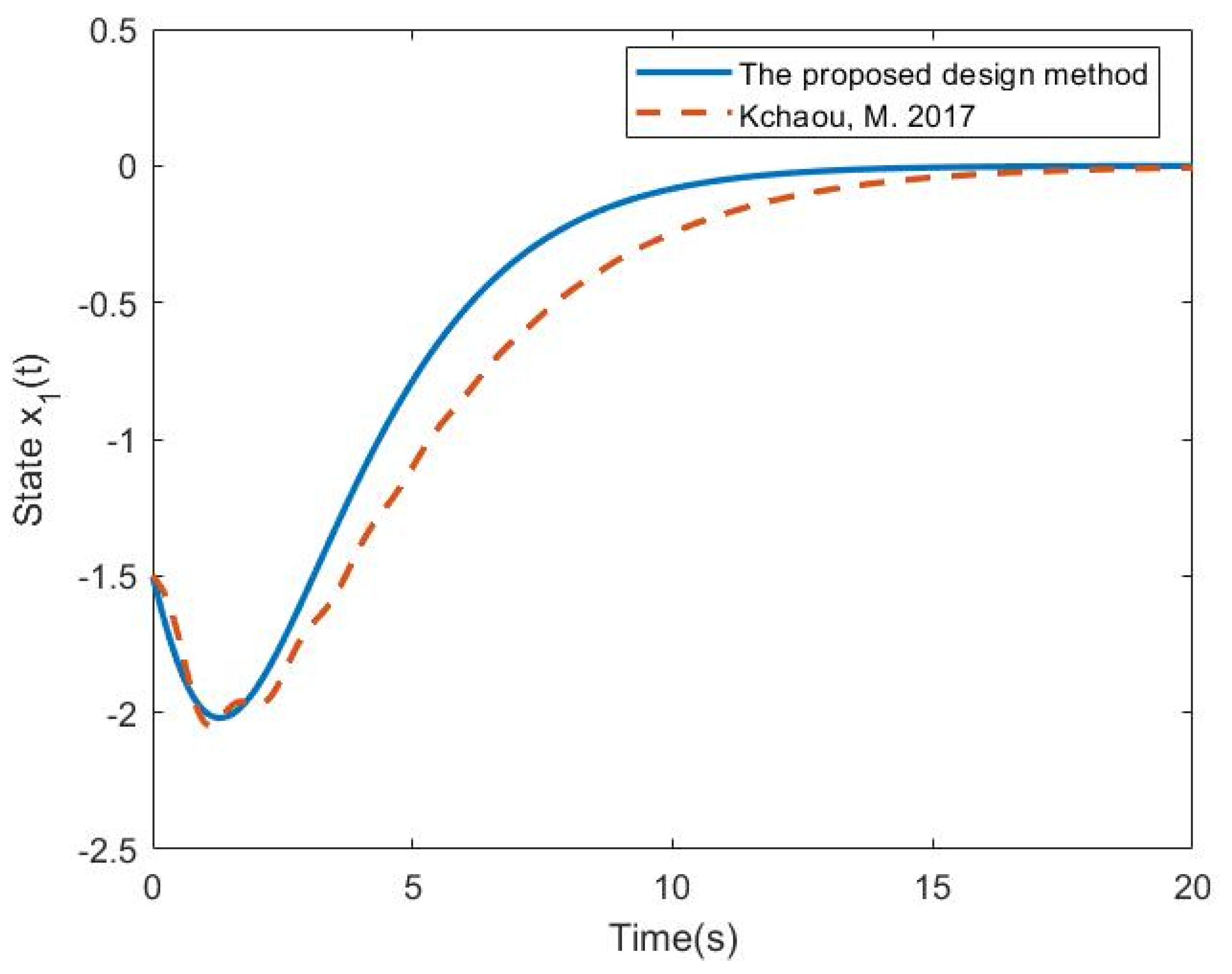
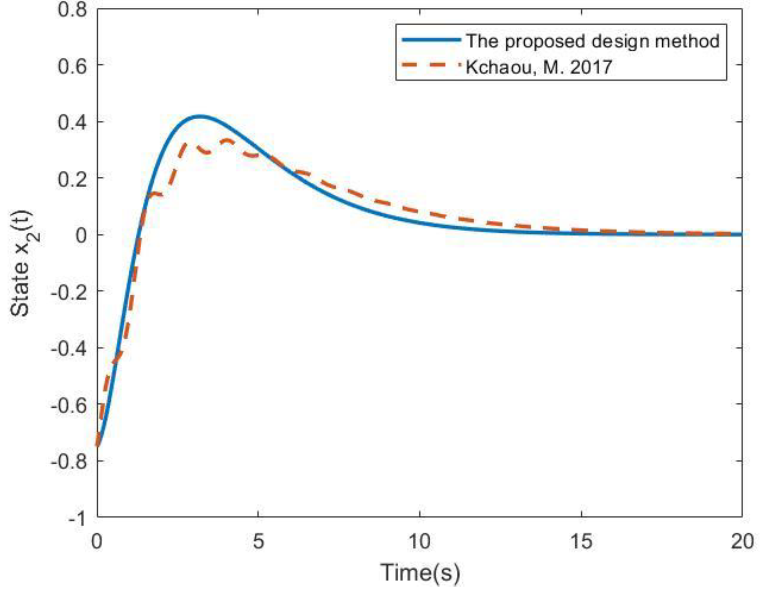
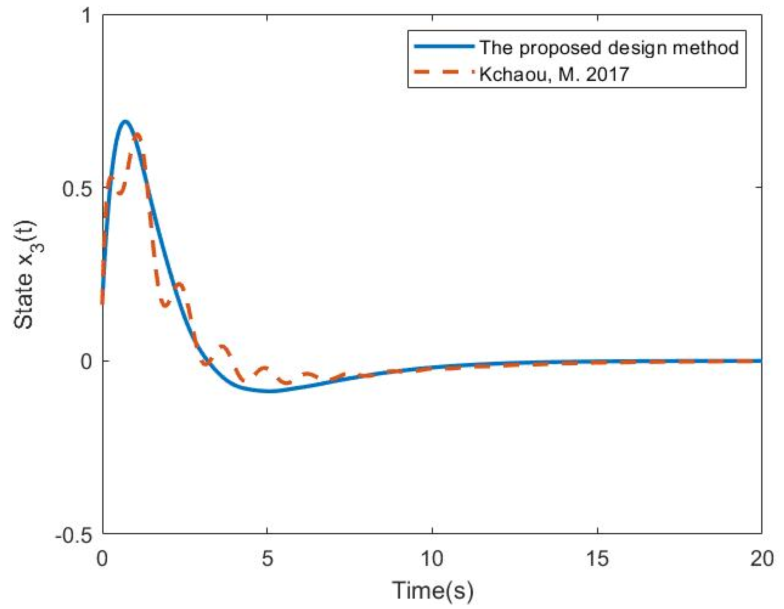
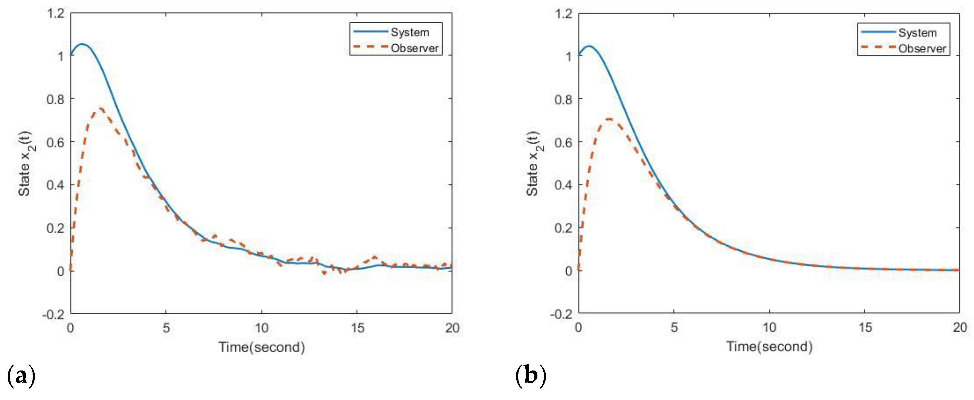
Given the initial conditions $x\left(0\right)={\left[\begin{array}{ccc}-1.5& -0.75& 0.17\end{array}\right]}^{\mathrm{T}}$ and $\widehat{x}\left(0\right)={\left[\begin{array}{ccc}0& 0& 0\end{array}\right]}^{\mathrm{T}}$, the state responses of the nonlinear singular system (34) are obtained in Figure 1, Figure 2 and Figure 3 by applying the OBPD Fuzzy Controller (7) with Gains (36) and Fuzzy Controller (38) with Gains (37), respectively. The figures show that the settling time obtained by the proposed design method is much better than the method in [29] despite the overshoot being slightly bigger. In order to verify the passive performance introduced in Definition 1, the following value is obtained based on the simulation results:

$$\frac{{\displaystyle {\int }_0^{t_p}{z}^{\mathrm{T}}\left(t\right)z\left(t\right)dt}+{\displaystyle {\int }_0^{t_p}{w}^{\mathrm{T}}\left(t\right)w\left(t\right)dt}}{2{\displaystyle {\int }_0^{t_p}{z}^{\mathrm{T}}\left(t\right)w\left(t\right)dt}}=0.9049$$

(39)

According to Definition 1, with the setting of matrices $S_1=1$, $S_2=0.9$, and $S_3=0.9$, it is obvious that the value in (39), which is smaller than 1.111, successfully satisfies the passive constraint in (12). That is, the attenuation performance of System (34) can be achieved with the external disturbance input energy. Because the passive constraint in (12) is satisfied, one can also see that the smoother responses of the system in (34) can be guaranteed by applying the fuzzy controller in (7).

Based on the comparison results in Example 1, it can be said that the proposed OBPD fuzzy controller design method can provide better control performance for the nonlinear singular system. Moreover, a more efficient stability analysis process can also be developed with the construction of a PD state feedback controller.

Example 2. 

The effectiveness of the proposed design method has been verified in Example 1. To further demonstrate the applicability and feasibility, the simulation results of a single-species bio-economic system are presented in the second example. Referring to [1], the following nonlinear system can be given by considering the economic interest of harvest effort in an immature population:

$$\begin{array}{l}{\dot{x}}_1\left(t\right)=\left(-\frac{\zeta \alpha }{r_2}-\frac{\eta c}{\rho }\right)x_1\left(t\right)+\zeta x_2\left(t\right)-\frac{c}{\rho }{x}_3\left(t\right)-\eta x_1^2\left(t\right)-x_1\left(t\right)x_3\left(t\right)+w\left(t\right)\end{array}$$

(40a)

$$\begin{array}{l}{\dot{x}}_2\left(t\right)=\alpha x_1\left(t\right)-r_2{x}_2\left(t\right)\end{array}$$

(40b)

$$0=\rho \left(\frac{\zeta \alpha }{r_2}-r_1-\alpha -\frac{\eta c}{\rho }\right)x_1\left(t\right)+\rho x_1\left(t\right)x_3\left(t\right)-m+u\left(t\right)$$

(40c)

where $x_1\left(t\right)={\Theta }_1\left(t\right)-\frac{c}{\rho }$, $x_2\left(t\right)={\Theta }_2\left(t\right)-\frac{\alpha c}{\rho r_2}$ and $x_3\left(t\right)=E\left(t\right)-\frac{\zeta \alpha \rho -\alpha \rho r_2-\rho r_1{r}_2-\eta c{r}_2}{\rho r_2}$. ${\Theta }_1\left(t\right)$ and ${\Theta }_2\left(t\right)$, respectively, represent the population density of juvenile species and adult species; $u\left(t\right)$ represents a policy for adjusting the tax; $\rho$ represents price constant per the individual population; $c$ represents the cost coefficient; and $m$ represents the economic interest of harvesting. Referring to [1], it is known that the bio-economic system has an equilibrium when $m=0$. More detail on the physical meaning of system parameters can be found in [1].

According to [1], the operating points are chosen as $x_1\left(t\right)\in \left[-10,10\right]$, and the system coefficients are selected as $\zeta =0.15$, $r_1=0.2$, $r_2=0.1$, $\alpha =0.5$, $\eta =0.001$, $\rho =1$, and $c=40$. To obtain more precise control performance, the problem of modeling error is also considered as the uncertain factor in the system. Then, the following T-S fuzzy model in (40) can be constructed:

$$E\dot{x}\left(t\right)={\displaystyle \sum _{i=1}^2{h}_i\left(x\left(t\right)\right)\left\{\left(A_i+\Delta A_i\right)x\left(t\right)+\left(B_i+\Delta B_i\right)u\left(t\right)+\left(D_i+\Delta D_i\right)w\left(t\right)\right\}}$$

(41a)

$$z\left(t\right)={\displaystyle \sum _{i=1}^2{h}_i\left(x\left(t\right)\right)\left\{C_{zi}x\left(t\right)+J_{i}w\left(t\right)\right\}}$$

(41b)

$$y\left(t\right)=Cx\left(t\right)$$

(41c)

where $E=\left[\begin{array}{ccc}1& 0& 0\\ 0& 1& 0\\ 0& 0& 0\end{array}\right]$, $A_1=\left[\begin{array}{ccc}-0.78& 0.15& -30\\ 0.5& -0.1& 0\\ 0.01& 0& -10\end{array}\right]$, $A_2=\left[\begin{array}{ccc}-0.8& 0.15& -50\\ 0.5& -0.1& 0\\ 0.01& 0& 10\end{array}\right]$, $B_i=\left[\begin{array}{c}0\\ 0\\ 1\end{array}\right]$, $C=\left[\begin{array}{ccc}1& 1& 0\\ 0& 0& 1\end{array}\right]$, $C_z=\left[\begin{array}{ccc}1& 0& 0\end{array}\right]$, $D_i=\left[\begin{array}{c}1\\ 0\\ 0\end{array}\right]$, $J_i=1$ for $i=1,2$, $\Delta A_1=\left[\begin{array}{ccc}-0.006sin\left(t\right)& 0.002sin\left(t\right)& 0\\ -0.015sin\left(t\right)& 0.005sin\left(t\right)& 0\\ 0& 0& 0\end{array}\right]$, $\Delta A_2=\left[\begin{array}{ccc}0.015sin\left(t\right)& -0.006sin\left(t\right)& 0\\ -0.005sin\left(t\right)& 0.002sin\left(t\right)& 0\\ 0& 0& 0\end{array}\right]$, $\Delta B_1=\left[\begin{array}{c}0\\ 0\\ -0.003sin\left(t\right)\end{array}\right]$, $\Delta B_2=\left[\begin{array}{c}0\\ 0\\ 0.004sin\left(t\right)\end{array}\right]$, $\Delta D_1=\left[\begin{array}{c}0.015sin\left(t\right)\\ 0\\ 0\end{array}\right]$ and $\Delta D_2=\left[\begin{array}{c}0.01sin\left(t\right)\\ 0\\ 0\end{array}\right]$. The membership functions of the fuzzy model in (41) are considered as $h_1\left(x\left(t\right)\right)=\frac{1}{2}\left(1-\frac{x_1\left(t\right)}{10}\right)$ and $h_2\left(x\left(t\right)\right)=1-h_1\left(x\left(t\right)\right)$. To develop the proposed design method, the following matrices are selected for uncertainties in the form of (2):

$$\begin{array}{l}{H}_{A1}=\left[\begin{array}{c}0.02\\ 0.05\\ 0\end{array}\right],H_{A2}=\left[\begin{array}{c}-0.03\\ 0.01\\ 0\end{array}\right],H_{B1}=\left[\begin{array}{c}0\\ 0\\ 0.01\end{array}\right],H_{B2}=\left[\begin{array}{c}0\\ 0\\ 0.02\end{array}\right],H_{D1}=\left[\begin{array}{c}0.03\\ 0\\ 0\end{array}\right],H_{D2}=\left[\begin{array}{c}0.05\\ 0\\ 0\end{array}\right],W_{A1}^{\mathrm{T}}=\left[\begin{array}{c}-0.3\\ 0.1\\ 0\end{array}\right],\\ W_{A2}^{\mathrm{T}}=\left[\begin{array}{c}-0.5\\ 0.2\\ 0\end{array}\right],W_{B1}=-0.3,W_{B2}=0.2,W_{D1}=0.5,W_{D2}=0.2\mathrm{and}\Delta \left(t\right)=sin\left(t\right)\end{array}$$

By setting the matrices $S_1=1$, $S_2=0.8$, $S_3=0.8$, and $\alpha =0.5$, the following gains can be obtained by solving Conditions (28) of Theorem 2:

$$\begin{array}{l}{F}_{p1}={10}^5\times \left[\begin{array}{ccc}0.0226& 0.0226& -1.1679\end{array}\right],F_{p2}={10}^5\times \left[\begin{array}{ccc}0.0256& 0.0256& -1.3219\end{array}\right],\\ F_{d1}={10}^4\times \left[\begin{array}{ccc}0.1513& 0.1513& -7.8155\end{array}\right],F_{d2}={10}^4\times \left[\begin{array}{ccc}0.1713& 0.1713& -8.8488\end{array}\right]\\ L_{p1}={10}^5\times \left[\begin{array}{cc}-0.0002& 0.0393\\ -0.0002& 0.0389\\ 0.0486& -2.5097\end{array}\right],L_{p2}={10}^5\times \left[\begin{array}{cc}-0.0001& 0.0317\\ -0.0001& 0.0317\\ 0.0491& -2.5340\end{array}\right]\\ L_{d1}={10}^5\times \left[\begin{array}{cc}-0.0001& 0.0221\\ -0.0001& 0.0213\\ 0.0236& -1.2184\end{array}\right]\mathrm{and}{L}_{d2}={10}^5\times \left[\begin{array}{cc}-0.0000& 0.0165\\ -0.0000& 0.0152\\ 0.0240& -1.2387\end{array}\right]\end{array}$$

(42)

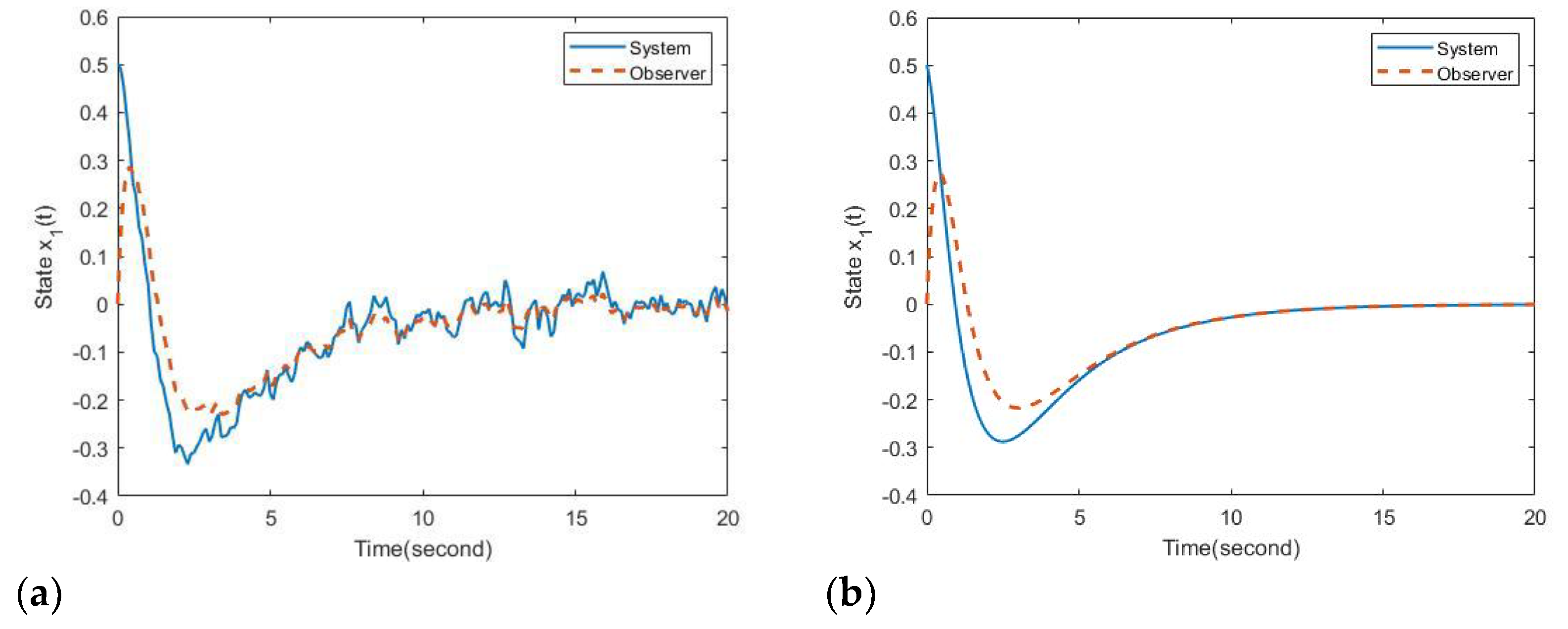
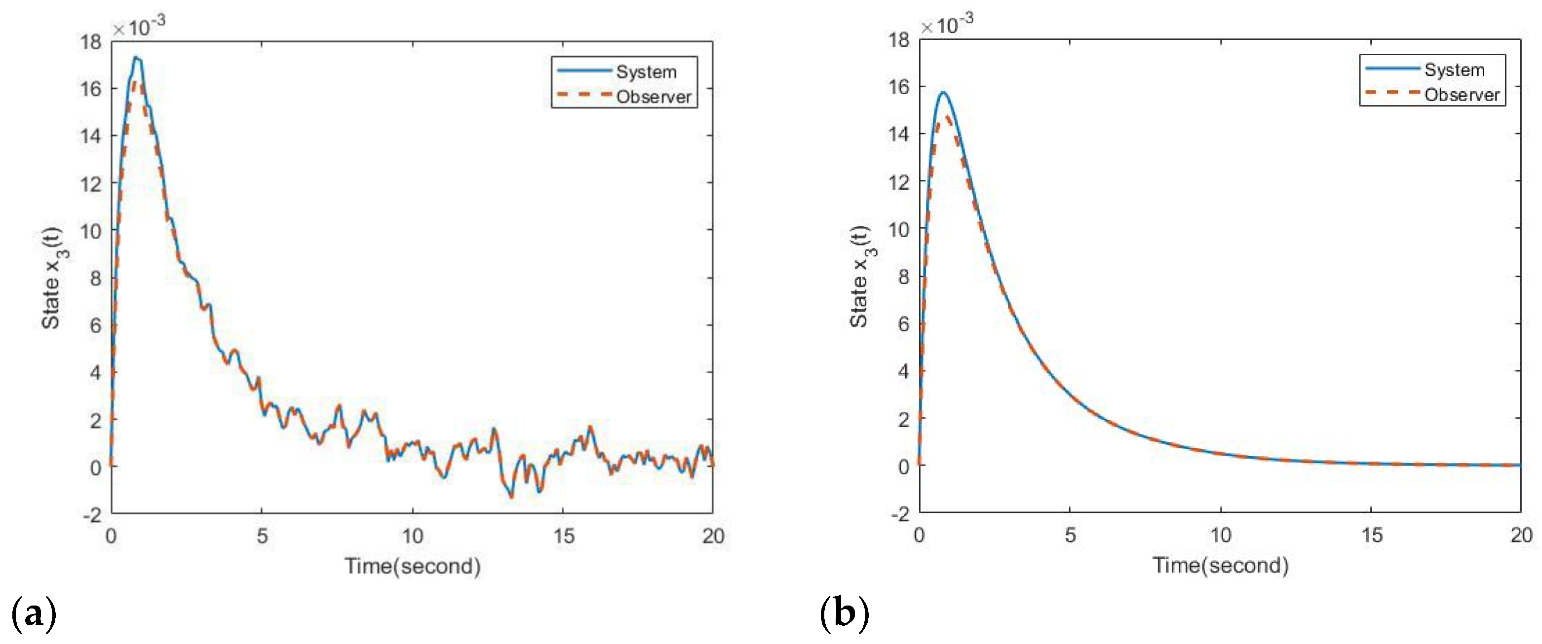
Based on the obtained gains, the proposed OBPD fuzzy controller in (7) can be designed for the nonlinear system in (40). The state responses of (40) are provided in Figure 4, Figure 5 and Figure 6 with the initial conditions $x\left(0\right)={\left[\begin{array}{ccc}0.5& 1& 0\end{array}\right]}^{\mathrm{T}}$ and $\widehat{x}\left(0\right)={\left[\begin{array}{ccc}0& 0& 0\end{array}\right]}^{\mathrm{T}}$. Based on the simulation results, the following value is also obtained to verify passive performance:

$$\frac{{\displaystyle {\int }_0^{t_p}{z}^{\mathrm{T}}\left(t\right)z\left(t\right)dt}+{\displaystyle {\int }_0^{t_p}{w}^{\mathrm{T}}\left(t\right)w\left(t\right)dt}}{2{\displaystyle {\int }_0^{t_p}{z}^{\mathrm{T}}\left(t\right)w\left(t\right)dt}}=0.94$$

(43)

Because the value of (43) is smaller than $1.111$, the constraint (12) of Definition 1 is satisfied, and the requirements of passivity are achieved. This means that even under the effect of the disturbance, the control performance also can be guaranteed for the system (40).

Referring to the figures, one can find that the stability of (40) is achieved by the proposed OBPD fuzzy controller (7). Moreover, the fuzzy observer can also successfully estimate the actual states. Based on the definition of state variables, the convergence of the bio-economy system in (40) means that all states can be controlled to a positive equilibrium. This result also indicates that the species population is guaranteed to be not endangered. Furthermore, government policy can efficiently adjust taxes to increase or decrease the cost of harvesting based on the proposed design method to achieve the sustainable development of bio-economic systems in (40). Thus, the proposed OBPD fuzzy controller design method can provide a valid choice for the control of numerical and practical nonlinear singular systems.

5. Conclusions

In this paper, an observer-based control problem was discussed for uncertain T-SFSS with external disturbance. According to the designed observer, the current states can be estimated to guarantee the existence of states in the controller. Therefore, the observer-based PD fuzzy controller can be applied to achieve the regularity and nonimpulsiveness of a system and guarantee the stability of considered systems when the complete states are not measurable. Based on passivity theory and Lyapunov theory, the stability conditions were obtained to deal with the control problem to achieve stability and attenuation performance. By utilizing SVD, projection lemma, and the Schur complement, the derived conditions were converted into strict LMI form, which can be effectively calculated by using convex optimization techniques. Furthermore, the positive definite matrix was not required as a diagonal case to reduce the conservatism of searching for feasible solutions. Based on the proposed method, the observer-based PD fuzzy controller can be designed to guarantee the stability of uncertain nonlinear singular systems subject to passivity. Finally, two examples have been presented to illustrate the effectiveness of the proposed control method.

References

1. Li, L.; Zhang, Q.; Zhu, B. Fuzzy Stochastic Optimal Guaranteed Cost Control of Bio-Economic Singular Markovian Jump Systems. IEEE Trans. Cybern. 2015, 45, 2512–2521. [Google Scholar] [CrossRef] [PubMed]
2. Zhai, D.; Zhang, Q.L.; Li, J.H. Fault detection for singular multiple time-delay systems with application to electrical circuit. J. Frankl. Inst. 2014, 351, 5411–5436. [Google Scholar] [CrossRef]
3. Qi, W.; Zong, G.; Karim, H.R. Observer-Based Adaptive SMC for Nonlinear Uncertain Singular Semi-Markov Jump Systems With Applications to DC Motor. IEEE Trans. Circuits Syst. I Regul. Pap. 2018, 65, 2951–2960. [Google Scholar] [CrossRef]
4. Mu, Y.; Zhang, H.; Sun, S.; Ren, J. Robust non-fragile proportional plus derivative state feedback control for a class of uncertain Takagi–Sugeno fuzzy singular systems. J. Frankl. Inst. 2019, 356, 6208–6225. [Google Scholar] [CrossRef]
5. Dai, L. (Ed.) Singular Control Systems; Springer: Berlin/Heidelberg, Germany, 1989. [Google Scholar]
6. Zhong, R.; Yang, Z. Delay-dependent robust control of descriptor systems with time delay. Asian J. Control. 2006, 8, 36–44. [Google Scholar] [CrossRef]
7. Zheng, Q.; Ling, Y.; Wei, L.; Zhang, H. Mixed H and passive control for linear switched systems via hybrid control approach. Int. J. Syst. Sci. 2018, 49, 818–832. [Google Scholar] [CrossRef]
8. Liu, Y.; Zhi, H.; Wei, J.; Zhu, X.; Zhu, Q. Event-triggered control for linear continuous switched singular systems. Appl. Math. Comput. 2020, 374, 125038. [Google Scholar] [CrossRef]
9. Takagi, T.; Sugeno, M. Fuzzy Identification of Systems and Its Applications to Modeling and Control. IEEE Trans. Syst. Man Cybern. 1985, 15, 116–132. [Google Scholar] [CrossRef]
10. Chang, W.; Su, C.; Varadarajan, V. Fuzzy controller design for nonlinear singular systems with external noises subject to passivity constraints. Asian J. Control. 2021, 23, 1195–1211. [Google Scholar] [CrossRef]
11. Chang, W.J.; Lian, K.Y.; Su, C.L.; Tsai, M.H. Multi-constrained Fuzzy Control for Perturbed T–S Fuzzy Singular Systems by Proportional-Plus-Derivative State Feedback Method. Int. J. Fuzzy Syst. 2021, 23, 1972–1985. [Google Scholar] [CrossRef]
12. Ku, C.C.; Chang, W.J.; Huang, Y.M. Robust Observer-Based Fuzzy Control Via Proportional Derivative Feedback Method for Singular Takagi–Sugeno Fuzzy Systems. Int. J. Fuzzy Syst. 2022, 24, 3349–3365. [Google Scholar] [CrossRef]
13. Wang, H.; Tanaka, K.; Griffin, M. An approach to fuzzy control of nonlinear systems: Stability and design issues. IEEE Trans. Fuzzy Syst. 1996, 4, 14–23. [Google Scholar] [CrossRef]
14. Ku, C.C.; Chang, W.J.; Huang, K.W. Novel Delay-Dependent Stabilization for Fuzzy Stochastic Systems with Multiplicative Noise Subject to Passivity Constraint. Processes 2021, 9, 1445. [Google Scholar] [CrossRef]
15. Qiao, H.Y.; Chang, W.; Lin, Y.; Lin, Y.W. Pole Location and Input Constrained Robust Fuzzy Control for T-S Fuzzy Models Subject to Passivity and Variance Requirements. Processes 2021, 9, 787. [Google Scholar] [CrossRef]
16. Chang, W.J.; Su, C.L.; Ku, C.C. Passive Decentralized Fuzzy Control for Takagi-Sugeno Fuzzy Model Based Large-Scale Descriptor Systems. IEEE Access 2022, 10, 28656–28669. [Google Scholar] [CrossRef]
17. Chang, W.J.; Liu, L.Z.; Ku, C.C. Passive fuzzy controller design via observer feedback for stochastic Takagi-Sugeno fuzzy models with multiplicative noises. Int. J. Control. Autom. Syst. 2011, 9, 550–557. [Google Scholar] [CrossRef]
18. Chang, W.J.; Lin, Y.W.; Lin, Y.H.; Pen, C.L.; Tsai, M.H. Actuator Saturated Fuzzy Controller Design for Interval Type-2 Takagi-Sugeno Fuzzy Models with Multiplicative Noises. Processes 2021, 9, 823. [Google Scholar] [CrossRef]
19. Lin, Y.H.; Chang, W.; Ku, C.C. Solving formation and containment control problem of non-linear multi-boiler systems based on interval type-2 Takagi-Sugeno fuzzy models. Processes 2022, 10, 1216. [Google Scholar] [CrossRef]
20. Su, C.L.; Chang, W.J.; Pen, C.L. Decentralized Multi-Performance Fuzzy Control for Nonlinear Large-Scale Descriptor Systems. Processes 2022, 10, 2578. [Google Scholar] [CrossRef]
21. Lu, Z.; Zhang, C.; Xu, F.; Wang, Z.; Wang, L. Fault Detection for Interval Type-2 T-S Fuzzy Networked Systems via Event-Triggered Control. Machines 2022, 10, 347. [Google Scholar] [CrossRef]
22. Zhang, B.; Liu, M.; Wang, K.; Tan, B.; Deng, Y.; Qin, A.; Liu, J. Takagi–Sugeno Fuzzy Model-Based Control for Semi-Active Cab Suspension Equipped with an Electromagnetic Damper and an Air Spring. Machines 2023, 11, 226. [Google Scholar] [CrossRef]
23. Liu, X.; Gao, Z.; Zhang, A. Observer-based fault estimation and tolerant control for stochastic Takagi–Sugeno fuzzy systems with Brownian parameter perturbations. Automatica 2019, 102, 137–149. [Google Scholar] [CrossRef]
24. Vafamand, N.; Asemani, M.H.; Khayatian, A. Robust L1 Observer-Based Non-PDC Controller Design for Persistent Bounded Disturbed TS Fuzzy Systems. IEEE Trans. Fuzzy Syst. 2017, 26, 1401–1413. [Google Scholar] [CrossRef]
25. Dong, J.; Yang, G.H. Observer-Based Output Feedback Control for Discrete-Time T-S Fuzzy Systems With Partly Immeasurable Premise Variables. IEEE Trans. Syst. Man, Cybern. Syst. 2016, 47, 98–110. [Google Scholar] [CrossRef]
26. Wang, X.L.; Yang, G.H. Observer-based fault detection for T-S fuzzy systems subject to measurement outliers. Neurocomputing 2019, 335, 21–36. [Google Scholar] [CrossRef]
27. Chang, W.J.; Lin, C.; Ku, C.C. Estimated state feedback fuzzy control for passive discrete time-delay multiplicative noised pendulum systems. J. Mar. Sci. Technol. 2015, 23, 98–108. [Google Scholar]
28. Ku, C.; Chen, G. New observer-based controller design for LPV stochastic systems with multiplicative noise. Int. J. Robust Nonlinear Control. 2019, 29, 4315–4327. [Google Scholar] [CrossRef]
29. Kchaou, M. Robust H observer-based control for a class of (TS) fuzzy descriptor systems with time-varying delay. Int. J. Fuzzy Syst. 2017, 19, 909–924. [Google Scholar] [CrossRef]
30. Wei, Z.; Ma, Y. Robust H observer-based sliding mode control for uncertain Takagi-Sugeno fuzzy descriptor systems with unmeasurable premise variables and time-varying delay. Inf. Sci. 2021, 566, 239–261. [Google Scholar] [CrossRef]
31. Liu, P.; Yang, W.T.; Yang, C.E. Robust observer-based output feedback control for fuzzy descriptor systems. Expert Syst. Appl. 2013, 40, 4503–4510. [Google Scholar] [CrossRef]
32. Ullah, R.; Li, Y.; Aslam, M.S.; Sheng, A. Event-Triggered Dissipative Observer-Based Control for Delay Dependent T–S Fuzzy Singular Systems. IEEE Access 2020, 8, 134276–134289. [Google Scholar] [CrossRef]
33. Mu, Y.; Zhang, H.; Sun, J.; Ren, J. Proportional plus derivative state feedback controller design for a class of fuzzy descriptor systems. Int. J. Syst. Sci. 2019, 50, 2249–2260. [Google Scholar] [CrossRef]
34. Mu, Y.; Zhang, H.; Su, H.; Wang, Y. Robust normalization and H stabilization for uncertain Takagi-Sugeno fuzzy singular systems with time-delays. Appl. Math. Comput. 2021, 388, 125534. [Google Scholar] [CrossRef]
35. Zhang, X.; Jin, K. Proportional Plus Derivative State Feedback Control of Takagi-Sugeno Fuzzy Singular Fractional Order Systems. Int. J. Control. Autom. Syst. 2021, 19, 3823–3829. [Google Scholar] [CrossRef]
36. Ku, C.C.; Chang, W.J.; Tsai, M.H.; Lee, Y.C. Observer-based proportional derivative fuzzy control for singular Takagi-Sugeno fuzzy systems. Inf. Sci. 2021, 570, 815–830. [Google Scholar] [CrossRef]
37. Chang, W.J.; Tsai, M.H.; Pen, C.L. Observer-Based Fuzzy Controller Design for Nonlinear Discrete-Time Singular Systems via Proportional Derivative Feedback Scheme. Appl. Sci. 2021, 11, 2833. [Google Scholar] [CrossRef]
38. Apkarian, P.; Tuan, H.; Bernussou, J. Continuous-time analysis, eigenstructure assignment, and H2 synthesis with enhanced linear matrix inequalities (LMI) characterizations. IEEE Trans. Autom. Control. 2001, 46, 1941–1946. [Google Scholar] [CrossRef]
39. Boyd, S.; El Ghaoui, L.; Feron, E.; Balakrishnan, V. Linear Matrix Inequalities in System and Control Theory; Society for Industrial and Applied Mathematics: Philadelphia, PA, USA, 1994; p. 15. [Google Scholar]
Figure 1. System responses of x 1 t in Example 1 [29].
Machines 11 00280 g001
Figure 2. System responses of x 2 t in Example 1 [29].
Machines 11 00280 g002
Figure 3. System responses of x 3 t in Example 1 [29].
Machines 11 00280 g003
Figure 4. Reponses of state x 1 t in Example 2: (a) with disturbance, (b) without disturbance.
Machines 11 00280 g004
Figure 5. Reponses of state x 2 t in Example 2: (a) with disturbance, (b) without disturbance.
Machines 11 00280 g005
Figure 6. Reponses of state x 3 t in Example 2: (a) with disturbance, (b) without disturbance.
Machines 11 00280 g006
Disclaimer/Publisher’s Note: The statements, opinions and data contained in all publications are solely those of the individual author(s) and contributor(s) and not of MDPI and/or the editor(s). MDPI and/or the editor(s) disclaim responsibility for any injury to people or property resulting from any ideas, methods, instructions or products referred to in the content.