Increased Dynamic Drivetrain Performance by Implementing a Modular Design with Decentralized Control Architecture

Abstract

This paper assesses the energy consumption, control performance, and application-specific functional requirements of a modular drivetrain in comparison to a benchmark drivetrain. A decentralised control architecture has been developed and validated using mechanical plant models. Simscape models have been validated with data from an experimental setup including an equivalent modular and benchmark drivetrain. In addition, the control strategy has been implemented and validated on the experimental setup. The results prove the ability of the control strategy to synchronize the motion of the different sliders, resulting in crank position tracking errors below 0.032 radians on the setup. The model and experimental data show an increased performance of the modular drivetrain compared to the benchmark drivetrain in terms of energy consumption, control performance, and functional requirements. The modular drivetrain is especially advantageous for machines running highly dynamic motion profiles due to the reduced inertia. For such motion profiles, an increased position tracking of up to 84% has been measured. In addition, it is shown that the modular drivetrain root mean square (RMS) torque is reduced with 32% compared to the benchmark drivetrain. However, these mechanical energy savings are partly counteracted by the higher motor losses seen in the modular drivetrain, resulting in potential electrical energy savings of around 29%.

1. Introduction

In the manufacturing industry, more stringent requirements are continuously set on operating machines and systems as a way to leverage manufacturers’ competitive advantages. Productivity, reliability, energy consumption, and flexibility are frequently recurring key performance indicators (KPI) for designing, developing, and selecting machines. The concept of modularity has been proposed [1,2,3] as a potential method to design and build machines with increased operational performance and customisation potential. The demand for easy customisation requires more flexibility in machine configuration. The literature has shown that modularity has benefits when it comes to developing more flexible machines [4,5]. A module-based approach can further reduce engineering and time costs [6], as scaling the system does not require a detailed redesign, instead relying on the addition or removal of modules built from standardized components. This paper adheres to the following definition of modularity [7]: the degree to which a system’s components may be separated and recombined, often enhancing the system’s scalability, flexibility, and variety of use cases. The unique set of separated and recombined components is called a module.

In [2], the authors showed that for direct drive systems a modular approach can result in increased operational efficiency. Furthermore, controller reference tracking outperformed the benchmark case, indicating the potential to push machines to higher operating speeds and thereby obtain an increased production rate. The benefits of introducing modularity have been illustrated for other applications as well, such as cranes [8], wind turbines [9], and electric vehicles [10,11]. For crane applications, ref. [8] showed that load-sharing electrical drive configurations result in a more uniform load distribution between motors and have the ability to eliminate crane skew. The grid connection of large wind turbines [9] can benefit from reduced capacitor voltage ripple when connected to a hybrid modular multilevel converter. For electric vehicle applications, ref. [11] demonstrated low harmonic distortion and high efficiency when implementing a modular multilevel topology using power electronics transformers.

This research paper aims to assess the performance of application cases for modular drivetrains typically used in tufting, weaving, and stamping machines. These machines often rely on the conversion of rotational motion to translational motion by means of bar and/or slider–crank mechanisms, which typically introduce a variable inertia. In [12], the authors demonstrated the robust performance of a slider–crank mechanism driven by a permanent magnet synchronous machine (PMSM) with an adaptive controller. However, this paper is limited to the motion control of a single slider–crank mechanism. Therefore, a modular drivetrain concept with six motors and slider-crank mechanisms (modules) is used as a test case to evaluate the performance of a decentralized control architecture for a modular drivetrain. Each independent drivetrain module executes a local control strategy without any information on the neighbouring modules. In addition, a benchmark (non-modular) drivetrain is developed in detail as a reference for a performance comparison. An experimental setup including the modular and benchmark drivetrain was designed and built, allowing the operational performance of the modular drivetrain system to be experimentally compared with the benchmark system.

Industrial weaving machines typically contain different functional components operating at high speeds, and each of their respective motion patterns must be synchronized to meet the machines’ functional requirements. Traditionally, these machines have a single motor that is mechanically linked to the machine load through bar linkages, cams, etc. This is equivalent to the benchmark drivetrain presented in this paper. The sliders of this benchmark drivetrain are inherently synchronized (neglecting the non-rigidity of crankshaft) by the mechanical design; ref. [13] already showed that the application of programmable controllers and electronic drive regulators can improve the operational efficiency and reliability of multi-motor machines in the textile industry. Modularity in drivetrain systems furthermore implies modifications in the control architecture. The motions of each individual module need to be electronically synchronized with each other in order to achieve the required motion of the load without causing unnecessary internal stresses or damage to the system. This topic has been discussed elaborately in previous research [14,15,16,17,18,19] for different kind of applications. In [16], for example, the authors applied the total sliding mode control method in order to synchronize multiple asynchronous machines. However, the above research focuses on centralized control architectures for synchronizing the modules, introducing the disadvantage of a single point of failure; if the controller fails, the entire drivetrain system fails to operate. For example, ref. [19] presented a speed control method for a dual PMSM connected in parallel and regulated with a single inverter. In [20], the author investigated a decentralised control strategy for synchronized control of multi-motor drive systems; however, his research was limited to a simulation environment and was not experimentally validated. Furthermore, the case of mechanically coupled motor loads, which are often present in textile machines, was not investigated. In contrast, the contributions of the present research include a performance analysis of a drivetrain system with mechanically linked loads. In practice, the six sliders are connected with an aluminum bar as the load. With respect to drivetrain modularization, this poses more stringent requirements on drivetrain control performance in order to avoid mechanical failures during drivetrain operation. Assuming a rigid system, multiple actuators provide control with a single degree of freedom. Along with implementing a modular mechanical design of the drivetrain system, this research further aims to implement a modular and scalable masterless control architecture. This paper describes a decentralised control architecture, aiming to avoid a single point of failure and allow continuous drivetrain operation in the event that the controller of a single module fails. The local module control strategy consists of cascaded proportional–integral (PI) loops and a feed-forward term. The dynamic drivetrain model in Matlab Simscape [21] allows this control strategy to be safely validated in a virtual environment before implementing and testing it on the experimental setup. To the best of our knowledge, introducing modularity in terms of both mechanical design and control architecture on a slider–crank drivetrain system with coupled loads represents a novel research approach.

The remainder of this paper is organised as follows. Section 2 introduces the theory, models, and methods used to design, develop, and implement the modular slider–crank drivetrain on both the system and component levels. Section 2.5 elaborates the design of the experimental setup and planned experiments used to assess the drivetrain performance. The model validation and drivetrain performance assessment are then discussed in Section 3, while Section 4 provides a final summary.

2. Materials and Methods

This section first elaborates on the methodology used to compare and assess the different drivetrain architectures. Second, the the concepts underlying the two drivetrain architectures under investigation are described. Third, the modelling of the drivetrain architectures and the control architecture and strategy are explained. Lastly, the design of the experimental setup is described in detail and the drivetrain KPIs are defined.

2.1. Assessment Methodology

The comparison of the drivetrains was executed following the principles illustrated in Figure 1. In [22], this methodology was explained and applied for the assessment of modular drivetrains in a simulation environment. Multiple drivetrain architectures have been conceptually designed and modelled. An architecture can consist of Z physical models, representing, for example, a slider–crank mechanism. The detailed simulation parameters are implemented in the simulation model. These may include physical component parameters, controller parameters, environmental conditions, etc. The simulation models are run with a certain load profile that defines the motion and external forces applied to the system. Furthermore, a set of key performance indicators are defined; using the output of the simulation models, the KPI values are calculated for the different drivetrain architectures, allowing a performance assessment and comparison to be carried out. Figure 1 focuses on a model-based performance assessment approach. This paper applies a similar methodology, using data from experimental setups instead of simulation models.

2.2. Drivetrain Architectures

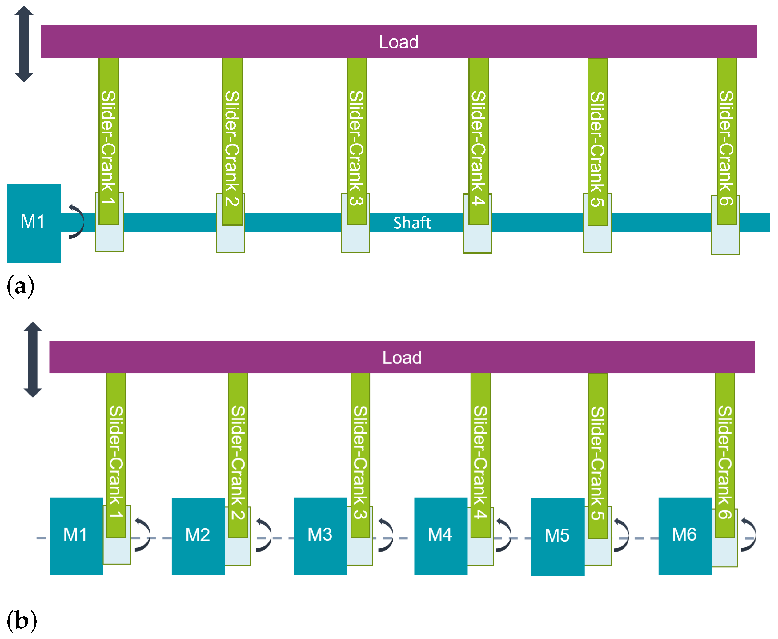
The definition of the modular drivetrain concept is based on the application of an industrial weaving (tufting) machine [1]. These machines make use of multiple slider–crank and/or multi-link bar mechanisms in parallel to convert rotational motion to translational motion on the load. In this case, the load is a uniformly-distributed mass connecting all of the sliders. Traditionally, these slider–crank mechanisms are connected by a crankshaft and driven by a single rotational power source, e.g., an electric motor. Figure 2 illustrates a simplified system architecture of this benchmark drivetrain with six slider–crank mechanisms. In [1], a novel modular alternative to this benchmark drivetrain was introduced, as shown schematically in Figure 2. This modular drivetrain architecture contains six slider–crank mechanisms, with the sliders all connected to a single load. This load is identical to the one in the benchmark drivetrain; however, each slider–crank mechanism is driven by a separate electric motor. Hence, the modular drivetrain system has six independently powered and controlled modules moving the load. This paper evaluates and compares the performance of both the benchmark and modular drivetrains by means of a dynamic mechanical model developed in Mathworks Simscape and an experimental test setup.

2.3. Drivetrain Models

The two system architectures depicted in Figure 2 were both modelled in the Matlab Simscape (R2019a) environment. Blocks from the Simscape foundation library were used, and custom Simscape blocks were developed as well. In order to build the models of the above-mentioned drivetrain systems, component models of the electric motor, slider–crank mechanism, and inertial load are required. The benchmark system architecture additionally requires modelling of the crankshaft. The different component models are described in more detail below.

The permanent magnet synchronous machine (PMSM) and its drive were simplified as a first-order system with rotational inertia and output torque saturated at the motor peak torque curve. In order to add a minimum of motor dynamics, a discrete low-pass filter was implemented. The transfer function for this filter allows the electromagnetic dynamic performance of the modelled motor to be limited by filtering the motor torque target $T_{Tgt}$ generated by the controller:

$$G=\frac{T_{Act}}{T_{Tgt}}=\frac{(t_s/\tau )z^{-1}}{1+(t_s/\tau -1)z^{-1}}$$

(1)

where $T_{Act}$ is the actual torque generated by the electric motor. The time constant $\tau$ is chosen such that the filter cutoff frequency (−6 dB) equals 800 Hz. Furthermore, the motor resolver data is modelled to include a communication delay and measurement noise. The delay is simple signal time delay between the resolver and the motor controller feedback loop (Section 2.4). White noise with a constant power spectral density (PSD) was superimposed on the crank resolver signal. The delay and noise values were fitted using experimental data of the setup, and are listed in

Table 1. Component properties.

Component	Parameter	Value	Units
AM8063L motor	Nominal power	4.97	$kW$
	Nominal torque	33.9	$Nm$
	Peak torque	111	$Nm$
	Torque constant	3.33	$Nm/A$
	Rotor inertia	29.0	$kg\times c{m}^2$
AM8051F motors	Nominal power	1.52	$kW$
	Nominal torque	5.8	$Nm$
	Peak torque	17.7	$Nm$
	Torque constant	1.77	$Nm/A$
	Rotor inertia	2.24	$kg\times c{m}^2$
Motor resolver	delay	1.1	$ms$
	Noise sample time	${10}^{-5}$	s
	Noise PSD	${10}^{-20}$	$Ma{g}^2/Hz$
Crankshaft	Inertia	$1.208\times {10}^{-3}$	$kg\times m^2$
	Length	1.96	m
	Torsional stiffness	$3.4\times {10}^3$	$Nm/rad$
	Torsional damping	0.02	$Nm\times s/rad$
Slider-crank	Crank length	20	$mm$
	Rod length	95	$mm$
	Crank inertia	12	$kg\times c{m}^2$
	Rod inertia	28	$kg\times c{m}^2$
	Crank mass	1.04	$kg$
	Rod mass	0.77	$kg$
	Slider friction coefficient	0.45	/
	Crank Coulomb friction	0.77	$Nm$
	Crank viscous friction	0.03	$Nm\times s/rad$
Load	Mass	4.42	$kg$
	Length	1.8	m
	Segment stiffness	$9.55\times {10}^5$	$N/m$
	Segment damping	8.29	$N\times s/m$

.

A separate Matlab script based on the power loss model of the PMSM, inverter, and cables was used to estimate the consumed electrical energy from the grid based on the measured (or simulated) motor speed and torque. The power loss model of the PMSM was defined by first establishing the current and voltage equations of a PMSM depending on the torque and speed setpoint [23], allowing efficiency maps to be computed by taking into account iron loss, copper loss, and mechanical loss [24] and validation to be carried out based on the efficiency maps provided by the the supplier. The motor performance characteristics were obtained from the datasheets of the PMSM motors used in the physical setup; more details can be found in Section 2.5. The cable Joule losses were directly computed from the motor currents and cable resistance. The inverter model was simplified through a load-dependent efficiency curve that was tuned to match the nominal loss from the suppliers’ datasheets.

In the benchmark drivetrain, the PMSM is connected to a crankshaft, as depicted in Figure 2. The crankshaft is driven by the electric motor, and connects the cranks of the six slider–crank mechanisms. The shaft was modelled based on the rotational stiffness, damping, and inertia.

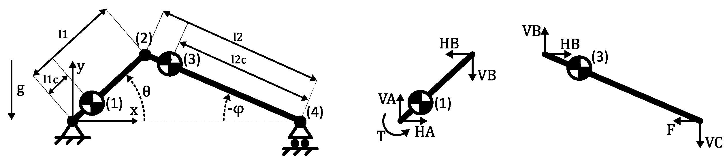
While the Simscape foundation library already collects a large set of component models, a detailed model for the slider–crank mechanism was lacking. First, the default Simscape slider–crank block does not include friction. Second, it does not include the effect of the position of the centre of gravity (Cog) of the crank and rod on the dynamic behavior. Third, gravity itself is unmodelled behaviour in the default Simscape block. Thus, the slider–crank mechanism [25] was analytically modelled and implemented in a custom Simscape block. The analytical equations included the kinematic and dynamic relationships between the rotational motion of the crank and the translational motion of the end of the rod (i.e., the slider) while taking into account the variable inertia effects. Second, the vertical and horizontal forces at the crankshaft, crank rod, and rod–load connections were calculated while taking into account the gravitational effects. All equations were derived based on the slider–crank free-body diagram depicted in Figure 3, and can be found in Appendix A.

The load consisted of an aluminium bar connecting the six sliders of the slider–crank mechanisms. For modelling purposes, the load was divided into five segments, with each located in between two slider–cranks. The segments were modelled using the lateral bending stiffness and damping along with the translational mass between the different sliders. The load’s total mass was determined on the basis of the mechanical CAD model and the lateral moment of inertia ($I_y=\mathrm{51,739}m{m}^4$), which is necessary in order to calculate the load segment stiffness. For each segment, the stiffness was separately calculated using the following equation:

$$K=\frac{1}{2}\times \frac{48\times E\times Iy}{2\times L_{segment}^3}$$

(2)

where E is the Young’s modulus, $I_y$ is the moment of inertia, and $L_{segment}$ is the length of the segment. The parameter values of the load are summarized in Table 1.

Additionally, static and kinetic frictions were taken into account in the model using a Simscape rotational friction element for the crank bearings and the translational friction for the slider carriage. The slider carriage friction model additionally took into account the total normal force acting on the slider carriage, including the gravitational force and the dynamic vertical force on the rod–load connection computed by the model of the slider–crank mechanism. The friction coefficients were determined by parameter optimization using experimental data from the setup (see Section 2.5), and are summarized in Table 1.

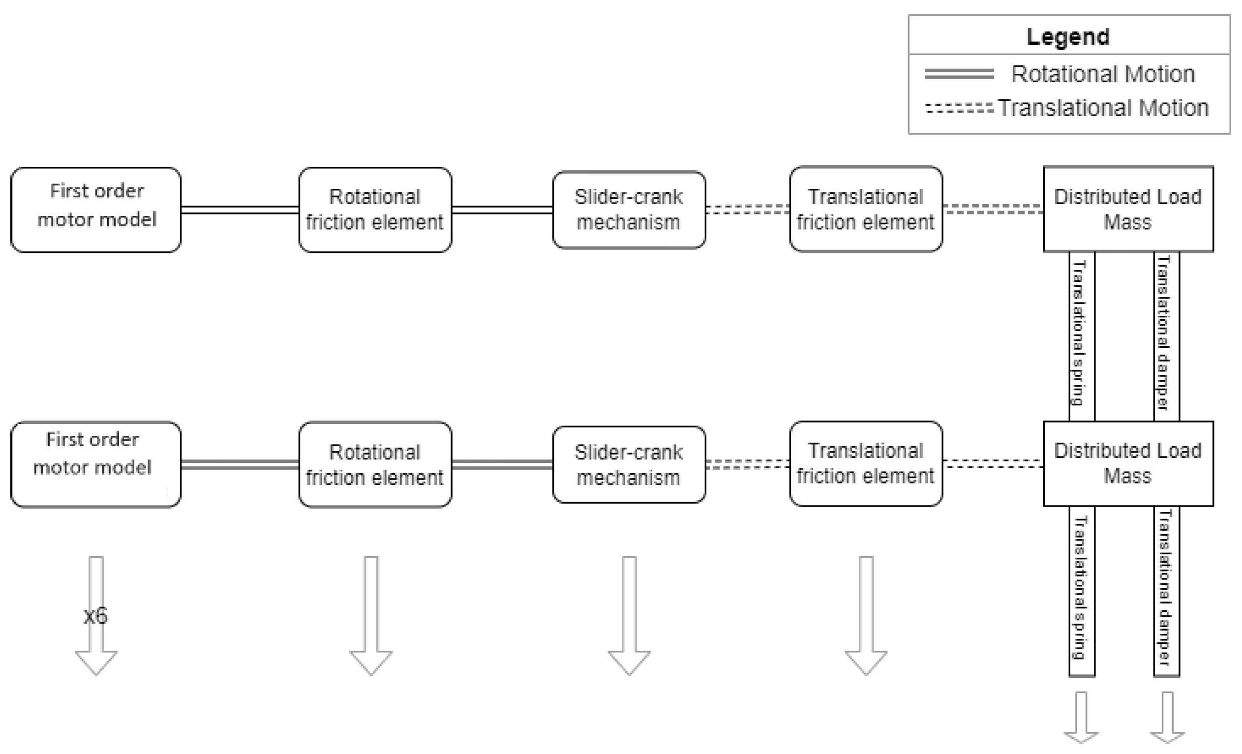
Figure 4 schematically shows how the modular drivetrain system model was built using the component models. The figure only shows two of the six modules. The benchmark drivetrain system model was built up equivalently, with the additional inclusion of a crankshaft model connecting all six cranks.

The main model parameters were defined from the component datasheets, and the friction parameters were tuned and validated by comparison with measurements taken on the physical setup. Table 1 provides the parameters values.

The mechanical system plant models of the benchmark and modular drivetrain were utilized to develop and validate the drivetrain control strategy, which is discussed in Section 2.4 below.

2.4. Control Architecture and Strategy

The sliders of the benchmark drivetrain are inherently synchronized by the presence of the crankshaft, which mechanically connects all six cranks. However, the modular drivetrain does not have mechanically linked slider–crank mechanisms, and as such the sliders have to be electronically synchronized through adequate control of all six motors.

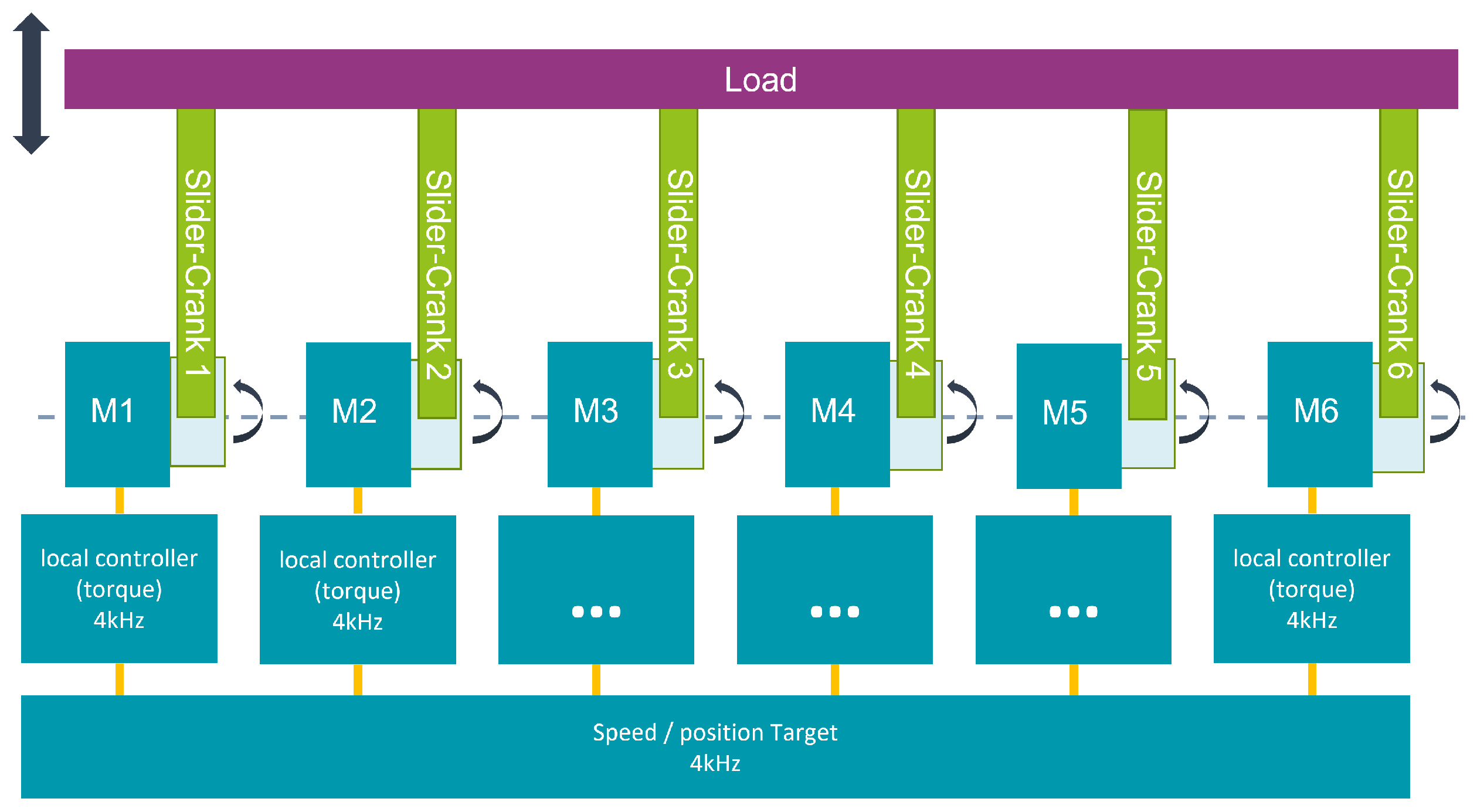
Previous research on control methods has shown good performance for multi-drive systems; however, the control architectures were largely implemented in a centralized manner [8,14,15,16,17,18], limiting the modularity to the mechanical design of the system. In this research, a decentralised control architecture for the modular drivetrain has been developed, with each motor being controlled locally. In this way, the concept of drivetrain modularity is further extended to the drivetrain control. In addition, removing the master controller scheme eliminates it as a potential single point of failure. A schematic of this control architecture is visualized in Figure 5. Each motor is controlled by a local controller with a sample time of 4 kHz. All local controllers act towards the same reference position and speed. This decentralised control architecture allows for increased system reliability and fault tolerance while maintaining synchronization of the six sliders.

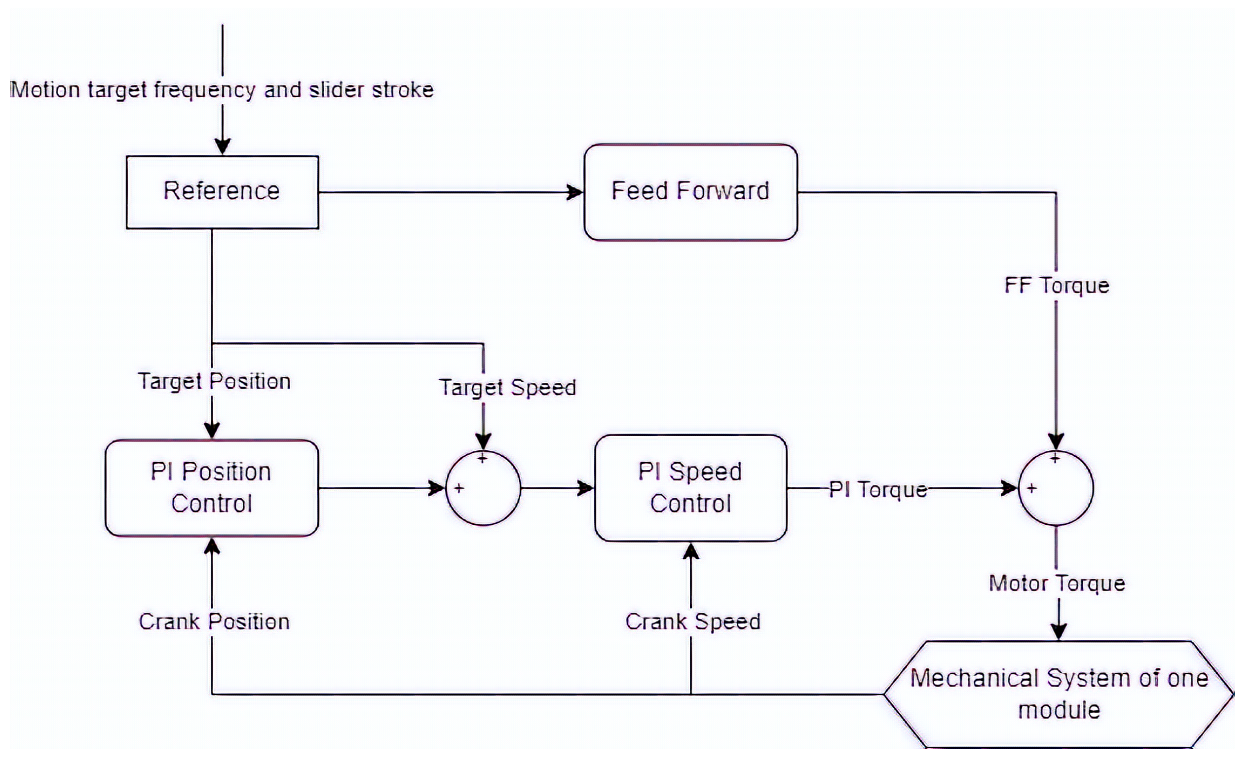
Both the benchmark and modular drivetrains were implemented with an identical local control strategy, which is visualized in Figure 6. While in the benchmark drivetrain only a single motor needs to be controlled, the modular drivetrain requires synchronized control of six independent motors. The applied control strategy is composed of the two main components depicted in Figure 6. First, a cascaded proportional integrator (PI) loop contains two PI feedback loops. This includes a positional PI controller which aims to track a rotational reference position for the motor. The output of this position controller is an input for the second PI loop, which aims to track a reference velocity. The proportional term of this velocity feedback loop is equivalent to the derivative term of a traditional PID feeback loop. Both PI loops include an anti-windup mechanism. The cascaded PI loop (position + velocity) was chosen over a traditional PID position controller because it enables sharing of the control parameter tuning between continuous and reciprocating motion (see Section 2.6 for definitions of continuous and reciprocating motion). For both drivetrains, the control parameters of the cascaded PI loop were optimized using the model-based PI tuning method. The control performance for each setup was numerically optimized for position and velocity tracking during high-speed operation.

Second, a feed-forward controller based on the analytic equations of the slider–crank mechanism (see Appendix A ) was implemented. This block outputs an estimation of the required motor torque for a certain reference crank position, velocity, acceleration, and slider–crank properties. The slider–crank properties include the dimensions, weight, inertia, and frictional characteristics of the mechanism. The exact properties and their values are listed in Table 1. The frictional characteristics were empirically defined using the experimental data from the setup, which is described below and is equivalent to the inverse of the slider–crank model described in Section 2.3.

The target motion time series is defined by a motion profile type, target slider frequency (number of slider cycles/second), and target stroke length (only applicable for the reciprocating motion type). Using the above two inputs, the reference block in Figure 6 computes the target crank position, velocity, and acceleration time traces for the different motion profile types under investigation. More information on these time-dependent motion profiles can be found in Section 2.6.

It is important to note that for the modular drivetrain, this control strategy needs to be applied in a decentralized manner; hence, each motor has its own local independent controller acting towards the same reference, resulting in a total of six active controllers. Such a decentralized control architecture eliminates the single point of failure and allows the system to remain functional (potentially with limited performance) in the event that a motor or its respective controller fails.

The combination of the mechanical plant models and control algorithm in the Matlab Simscape environment allows the performance of both the modular and non-modular (benchmark) system architectures to be virtually evaluated. Next, we aimed to further validate these findings with experimental results. Therefore, an experimental setup was developed and built, which is described in the next section.

2.5. Design of Experimental Setup

A mechanical design and component selection process was executed based on the conceptual diagrams of the system architectures visualized in Figure 2.

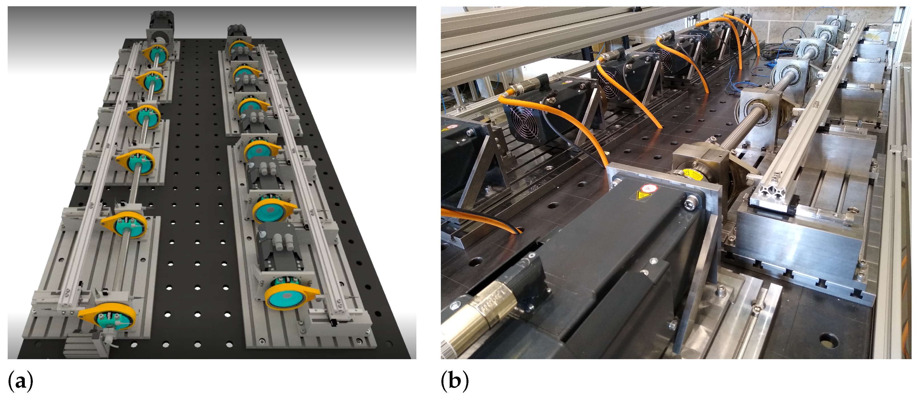
The setup is visualized in Figure 7 and its operation is demonstrated in the video provided in [26]. Both the modular and benchmark drivetrain were installed on the same Welda test bed table and rotated in opposite directions, resulting in the inertial forces of both setups being counterbalanced, thereby reducing the vibrations and swinging of the table. However, this has the negative consequence that a single drivetrain cannot be operated individually at high speeds, inhibiting the experimental evaluation of the maximum operating speed of the fastest drivetrain. The Welda table was installed with multiple T-slot plates, allowing for easy and flexible mounting of all components on the table. This mounting flexibility and freedom is particularly important for the modular drivetrain, as the mechanical alignment of the six modules is both challenging and critical for proper operation. For the benchmark drivetrain, the six slider–crank mechanisms were inherently aligned (within design tolerances) by the presence of the crankshaft.

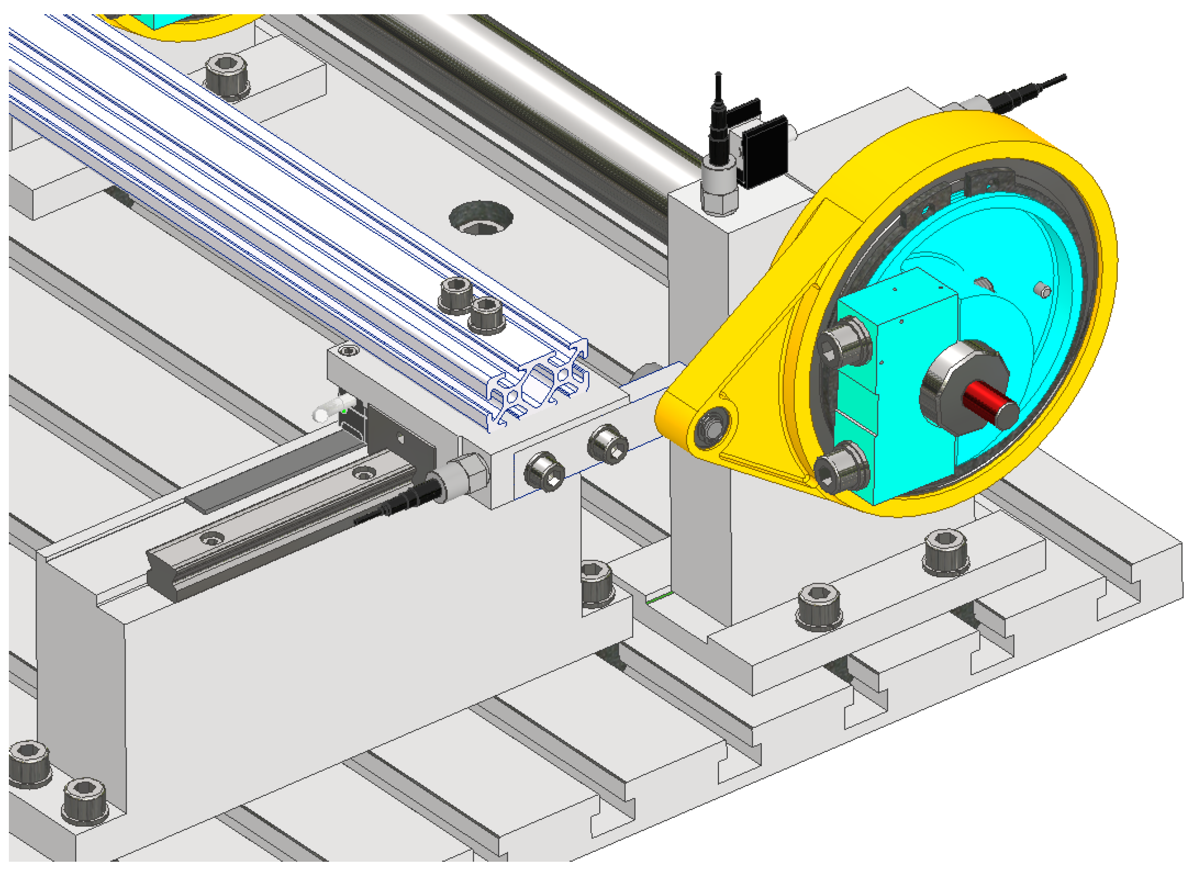
To keep the research industrially relevant, component sizing and selection focused primarily on off-the-shelf components. The modular drivetrain used six AM8051F motors, while the benchmark drivetrain used a single AM8063L motor. Table 1 lists several basic properties of these motors. The motors’ front faces were bolted onto a steel frame. This steel frame had slots in the bottom to affix the frame to the test bed using the T-slots, allowing for a range of movement when positioning the motors. This range of movement is particularly important for the modular drivetrain, as it has no crankshaft connecting all modules, meaning that the six slider–crank mechanisms are not inherently mechanically aligned. Custom alignment tools were developed together with a specific alignment procedure to achieve mechanical alignment within tolerances. The slider carriage was a caged ball linear guide of THK (SSR 15 X W 1 SS QZ + 160 L), and is shown in Figure 8. The load bar connecting all six slider carriages was a standard aluminum item profile with a total weight of 4.42 kg. All electronic components, such as the motor drives, IPC, IO cards, and low-voltage power supply, were stock components. A total of four type AX5000 Beckhoff drives were installed in the electrical cabinet: a single drive for the benchmark drivetrain, and three dual-channel drives for the modular drivetrain. For the latter dual-channel drives, the two channels were separated, allowing independent control of the six motors of the modular drivetrain. Each drive was operated at a switching frequency of 8 kHz. The IPC implemented and ran the control algorithm, as discussed in Section 2.4, at a sample frequency of 4 kHz. The IPC then sent the individual torque targets to each drive over an EtherCAT communication network.

The main custom components of the setup were the crankshaft and the slider–crank mechanism. The crankshaft was a custom machined steel rod connecting the motor to the six slider–crank mechanisms of the benchmark drivetrain. The modular drivetrain did not have this crankshaft. All slider–crank mechanisms were identical by design. The mechanism was composed of an eccentric bearing converting the rotational motion to translational motion. The eccentricity of the bearing was obtained by offsetting the bearing’s centre axis with respect to the rotational axis. The eccentric bearing is visualized in more detail in Figure 8. The slider–crank mechanism had a crank length of 20 mm, allowing a maximum full slider stroke of 40 mm to be achieved. The dimensions and properties of the main off-the-shelf and custom components are listed in Table 1.

2.6. Performance KPIs

The availability of a simulation environment and experimental environment allowed an accurate performance assessment of the benchmark and modular drivetrains to be carried out.

The following KPIs were defined for evaluating the performance of both drivetrain systems following the approach described in Section 2.1.

The maximum torque required for a certain operating condition is an indicator of the peak load of a drivetrain system. A lower peak load results in higher system reliability and lifetime. The crank torque is calculated on the basis of the motor currents reported by the respective drive. The following equation was applied for field-oriented controlled (FOC) PMSM:

$$T\left(t\right)=k_t\ast i_q\left(t\right)$$

(3)

where $k_t$ and $i_q\left(t\right)$ are the motor torque constant and the motor q-axis current, respectively. Next, the maximum torque for a time series torque signal is calculated as follows:

$$T_{max}=max(\parallel T\left(t\right)\parallel )$$

(4)

For the modular drivetrain, $T\left(t\right)$ is the total drivetrain torque, which is equal to the sum of the torques of the six independent motors.

RMS torque allows the mechanical energy consumption of the system drivetrains to be compared for a given motion profile.

$$T_{rms}=\sqrt{mean\left(T{\left(t\right)}^2\right)}$$

(5)

The crank position control error defines the control accuracy of the system drivetrain. The crank position is measured by the motor resolvers and read out from the drives. Based on these resolver signals, the KPI is calculated as follows.

$$e_{\theta }^{max}=max\{\parallel \left({\theta }_{act}\left(t\right)-{\theta }_{ref}\left(t\right)\right)\parallel \}$$

(6)

The slider error defines how accurately the slider positions are aligned and synchronized with each other during motion. For an ideal drivetrain (meaning one without disturbances such as misalignment and other design tolerances), this largely correlates with the above-mentioned crank position control error; however, for a non-ideal system such as the experimental setup, this is not necessarily the case. In practice, design tolerances, mounting misalignments, etc., are inherently present. The slider positions are measured using linear encoders (RLS LA11) attached to the slider carriage. Based on these measurements, the maximum slider error is calculated as follows:

$$e_{sliderPos}^{max}=\underset{tϵ[t_0,t_{end}]}{max}\{\parallel \underset{iϵ[1,6]}{max}\left\{P{S}_{i,t}\right\}-\underset{iϵ[1,6]}{min}\left\{P{S}_{i,t}\right\}\parallel \}$$

(7)

where $P{S}_{i,t}$ is the position of slider number i at instant t, $t_0$ is the start time of the experiment with the machine at steady speed, and $t_{end}$ is the end of the experiment.

The RMS electrical power defines the average power drawn from the electrical grid for a certain motion profile. The instantaneous electrical power $P^{elec}\left(t\right)$ is estimated using the motor, inverter, and cable loss models, which require the motor speed and torque as inputs. For accurate estimation of the electrical energy consumption, the measured speed and estimated torque signals of the setup experiments are used as inputs to the loss models. The RMS electrical power consumption for a certain motion profile is calculated as follows.

$$P_{rms}^{elec}=\sqrt{mean\left(P^{elec}{\left(t\right)}^2\right)}$$

(8)

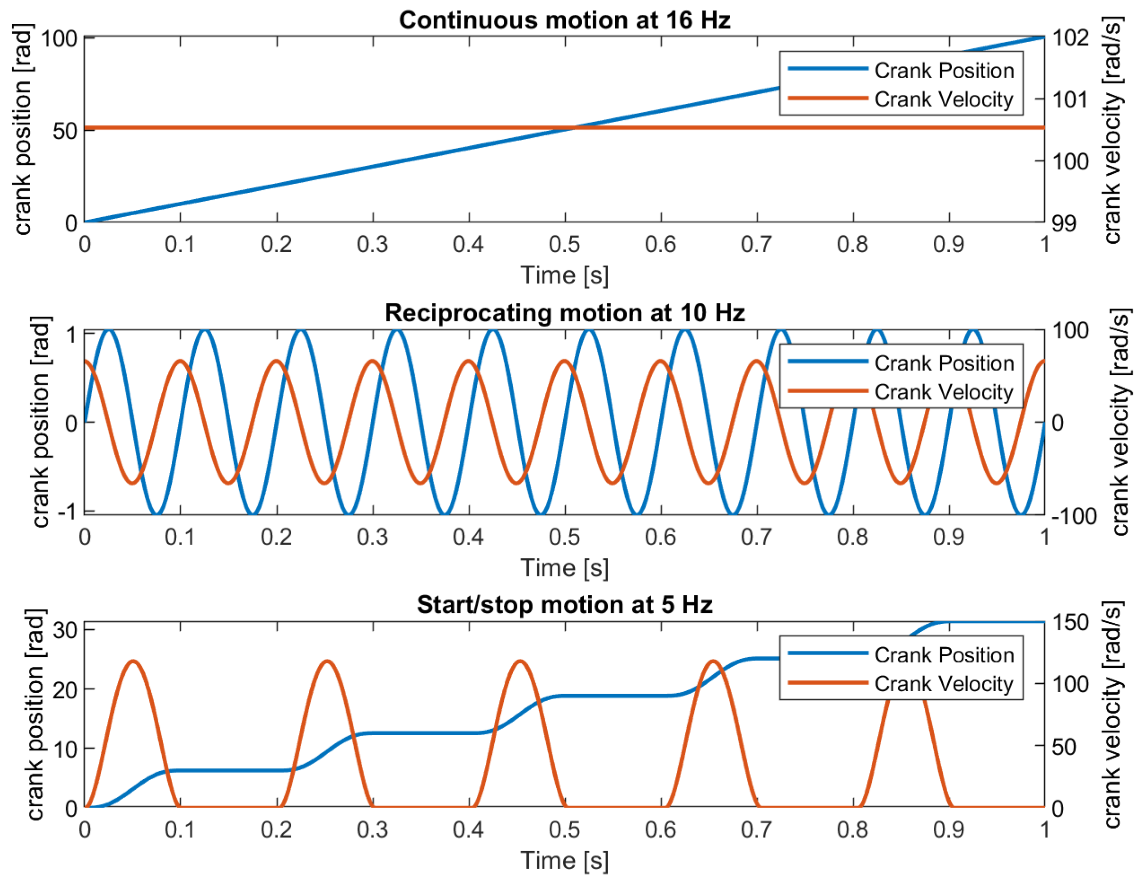
The performance comparison using the above KPIs of the benchmark and modular system drivetrain was performed for an equal load profile (see Figure 1). The performance was investigated for three different motion profiles: continuous motion, reciprocating motion, and start/stop motion. In the continuous motion profile, the crankshaft continuously rotates in one direction at a constant speed. The start/stop motion rotates the crankshaft in one direction as well, except that the shaft stops rotating every full cycle with a duty cycle of 50%. This motion profile is typical for pick-and-place applications. In reciprocating motion, the crankshaft smoothly oscillates in two directions, which means that the motor operates in both positive and negative speed ranges. Examples of these different motion profiles are visualised in Figure 9 for the crank. It is clear that both the reciprocating and start/stop motion profiles are far more dynamic and introduce higher acceleration than the more stationary continuous motion profile. Both the continuous motion and start/stop motion profiles have a fixed stroke length, i.e., the maximum stroke is defined by the mechanical design. The reciprocating motion profile has the additional benefit of providing an electronically controllable stroke length, meaning that the stroke length is determined by the amplitude of the sinusoidal crank position time signal.

3. Results and Discussion

3.1. Simulation Versus Experimental Results

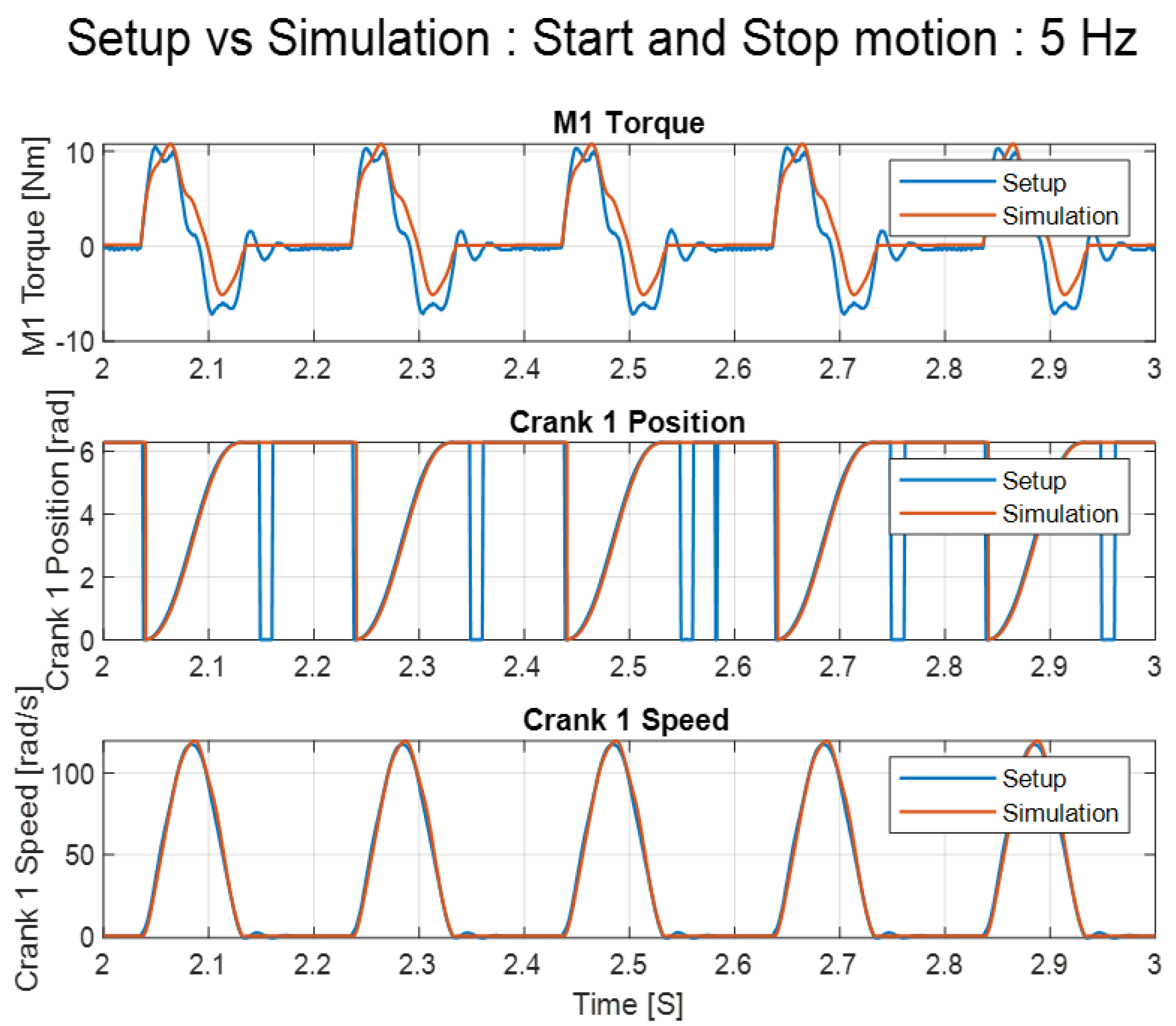
A first analysis was carried out to compare the simulation results with the experimental results for both the modular and benchmark drivetrains. For the continuous, reciprocating, and start/stop motion profiles, the above mentioned KPIs were compared using a fixed slider motion frequency of 16 Hz, 10 Hz, and 5 Hz, respectively. These operational frequencies are close to the maximum obtainable operational frequencies of the experimental benchmark drivetrain for the continuous, reciprocating and start/stop motion profiles, respectively. Figure 10 shows a comparison of the results for the modular drivetrain running the start/stop motion profile. The accuracy of the simulation estimation for each KPI is calculated as follows:

$$accurac{y}_{pct}=(1+(KP{I}_{sim}-KP{I}_{exp})/KP{I}_{exp})\ast 100$$

(9)

The resulting accuracy is a percentage value, where 100 percent indicates a perfect match between simulation and experiment.

All analysis results are summarized in

Table 2. Modular drivetrain: simulation versus experiment.

KPI		Reciprocating	Continuous	Start/Stop
		10 Hz	16 Hz	5 Hz
RMS torque	simulation	32 Nm	27 Nm	28 Nm
	experiment	38 Nm	13 Nm	28 Nm
	accuracy	83%	202%	98%
Max torque	simulation	51 Nm	42 Nm	67 Nm
	experiment	57 Nm	23 Nm	64 Nm
	accuracy	90%	183%	105%
Max crank error	simulation	0.018 rad	0.025 rad	0.026 rad
	experiment	0.032 rad	0.019 rad	0.022 rad
	accuracy	56%	132%	122%

and

Table 3. Benchmark drivetrain: simulation versus experiment.

KPI		Reciprocating	Continuous	Start/Stop
		10 Hz	16 Hz	5 Hz
RMS torque	simulation	42 Nm	32 Nm	32 Nm
	experiment	57 Nm	13 Nm	41 Nm
	accuracy	74%	235%	76%
Max torque	simulation	59 Nm	40 Nm	85 Nm
	experiment	98 Nm	28 Nm	108 Nm
	accuracy	60%	145%	79%
Max crank error	simulation	0.071 rad	0.067 rad	0.111 rad
	experiment	0.160 rad	0.023 rad	0.135 rad
	accuracy	45%	286%	82%

.

The slider error is not analysed in the tables, as the simulation was assumed to be ideal in the sense that mechanical misalignment or design tolerances were not included in the model. The electrical power consumption is not included either, as the sensors required for electrical measurements were not installed in the experimental setup.

The results show accurate torque estimation of the models for both the start/stop motion and reciprocating motion profiles. This can be clearly seen in Figure 10 for the modular drivetrain running the start/stop motion profile, and is reflected in the comparison of RMS and maximum torque as well. For example, in Table 2, a 98% fit for the RMS torque of the modular drivetrain running the start/stop motion profile can be observed. A less accurate fit is observed for the continuous motion profile, with an accuracy of only about 200% when estimating the RMS and maximum torque. This can be explained by the need to analyse the different terms of the total required torque for the three motion profiles. The total torque amount consists of the inertial torque, gravity torque, and friction torque. The model relies on accurate analytic, kinematic, and dynamic equations for estimating the inertial and gravity torque based on known design parameters such as the geometry, mass, and inertia. These parameters are easily measured and/or calculated with a high degree of confidence. However, the friction torque is far more difficult to predict, and is a source of uncertainty. Although the friction parameters were fitted using measured data, the friction model can be further improved. For example, a large temperature dependency of the friction torque on the setup was observed. The current model does not include a thermal domain, which would help to estimate component temperatures. As our model does not include temperature-dependent friction, its estimation of the friction torque is far less accurate than that of the inertial and gravity torque. Start/stop and reciprocating motion are highly dynamic motion profiles causing high inertial torque values. As a result, the total required torque for these motion profiles is dominated by the inertial torque, meaning that the ratio of the accurately estimated inertial torque over the less accurately estimated friction torque is fairly high. This explains the better torque estimation results for the more dynamic start/stop and reciprocating motion profiles.

The same reasoning applies when comparing the torque estimation accuracy of the modular and benchmark drivetrains. The results in Table 2 and Table 3 generally show a better model fit for the modular drivetrain. The benchmark drivetrain design includes a crankshaft and supporting bearings, while the modular drivetrain does not have these components. Our experimental observations using the testing setup show a significant amount of friction in these grease-lubricated supporting bearings of the crankshaft on the benchmark drivetrain. Accordingly, the frictional torque is higher for the benchmark, resulting in lower model accuracy for this drivetrain.

3.2. Performance Comparison of the Benchmark and Modular Drivetrains

This subsection focuses on a technical performance comparison between the modular and benchmark drivetrains. Similar to the previous subsection, the performance of both drivetrains was analyzed for the three different motion profiles with the modular and benchmark drivetrains running simultaneously at the same speed.

Table 4. Performance comparison.

KPI		Reciprocating	Continuous	Start/Stop
		10 Hz	16 Hz	5 Hz
RMS torque	Benchmark	57 Nm	13 Nm	41 Nm
	Modular	38 Nm	13 Nm	28 Nm
	Delta	−33%	−2%	−32%
Max torque	Benchmark	98 Nm	28 Nm	108 Nm
	Modular	57 Nm	23 Nm	64 Nm
	Delta	−42%	−18%	−41%
Max crank error	Benchmark	0.160 rad	0.023 rad	0.135 rad
	Modular	0.032 rad	0.019 rad	0.022
	Delta	−80%	−9%	−84%
Max slider error	Benchmark	0.43 mm	0.95 mm	0.46 mm
	Modular	0.39 mm	0.83 mm	0.41 mm
	Delta	−9%	−13%	−11%
RMS electrical power	Benchmark	3.58	2.01	5.17
	Modular	3.1	2.2	3.68
	Delta	−13%	+9%	−29%

shows the resulting KPI values of both drivetrains for each motion profile and the KPI differences between the modular drivetrain and the benchmark drivetrain in percentages. All KPI values shown in the table were directly derived from experimental data except for the RMS electrical power.

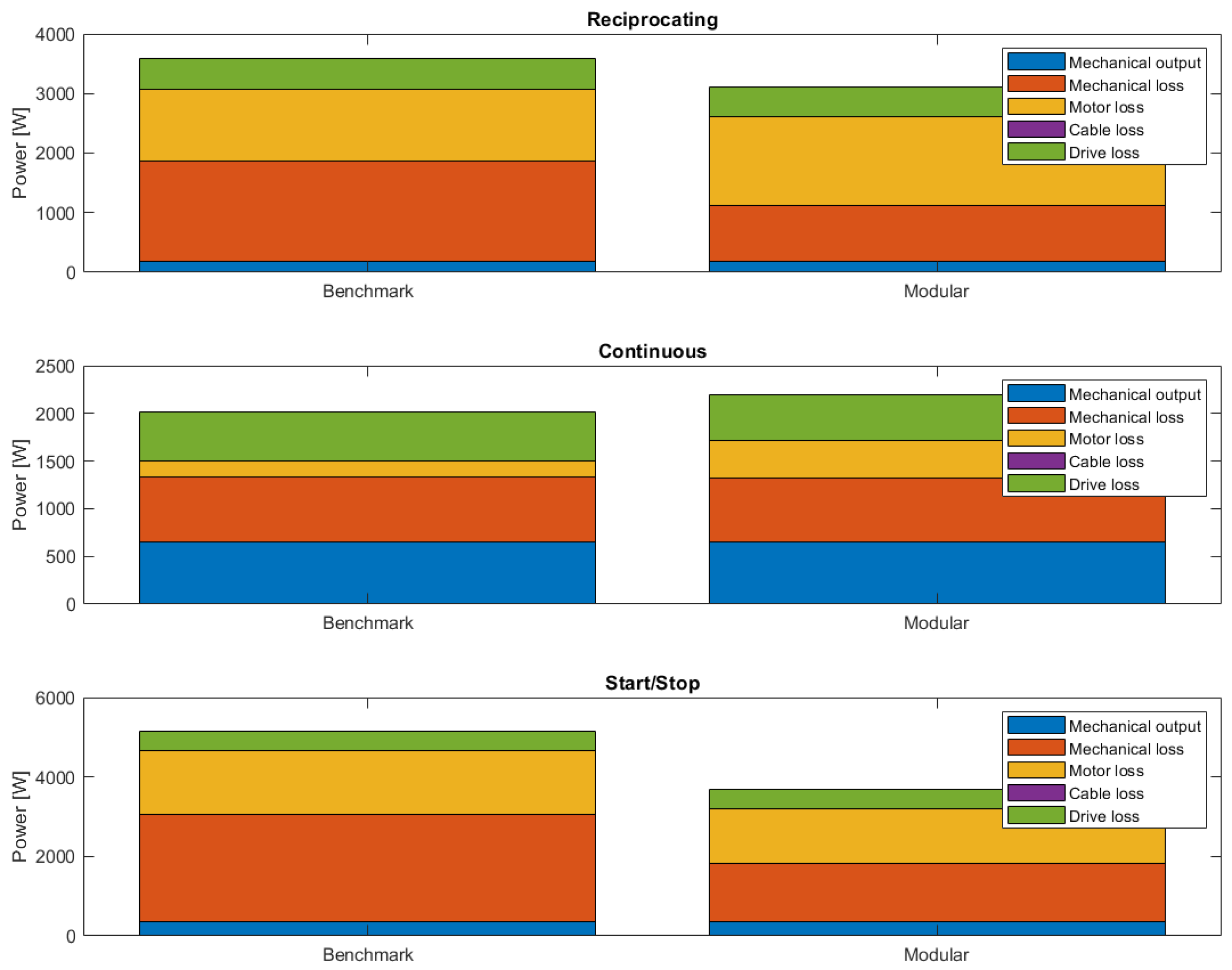
For the continuous motion profile, the measurements show only a minor reduction of 2% in the RMS torque required to run the motion cycle. The maximum observed torque is reduced by about 18%. Hence, while the peak load of the modular drivetrain is clearly reduced, the average mechanical power delivered by the motors in the continuous motion profile is not significantly altered. Unfortunately, the electrical power consumption of the modular drivetrain is 9% higher than the benchmark drivetrain. Figure 11 shows that this can be explained by the increased overall motor losses of the six smaller motors compared to the motor loss of the single motor in the benchmark drivetrain. Furthermore, the experimental results shows a 19% increase in the position tracking performance of the modular drivetrain compared with the benchmark. As a result, the maximum slider error is reduced by 13%.

More significant performance improvements are experimentally observed for the reciprocating and start/stop motions. The total RMS torque delivered by the six modular motors is up to 33% lower compared to the RMS torque delivered by the single motor of the benchmark drivetrain. The maximum torque is decreased by up to 42%, resulting in lower fatigue stress on the modular drivetrain. As a result, for these more dynamic (high-acceleration) motion profiles, significantly less average mechanical power is required to drive the modular system compared to the benchmark system. In addition, a reduction in electrical energy consumption of up to 29% is estimated, and an 84% reduction in the tracking error is observed. Having the system load distributed over the six actuators helps to achieve better control performance. As a consequence, the slider error is reduced due to mechanical play in the pin connection between the slider and the rod, albeit less drastically, up to 11%.

These experimental results demonstrate that a modular drivetrain can result in better tracking performance, lower peak system loads, and reduced average mechanical and electrical power consumption with respect to the standard non-modular drivetrains currently used by industry. This is especially true for highly dynamic motion profiles with large acceleration values, which can benefit from a mechanical system with reduced inertia.

3.3. Outlook

Improvements could be made to both the testing setup and the model. The accuracy of the friction model could be increased by including the thermal domain. For validation of thermal behavior, temperature sensors would need to be added to the setup. In order to analyse the high-frequency system dynamics (>1 kHz), the simulation environment could benefit from a detailed model of the motor drive that includes current control.

Interesting future work could include the application of novel robust control techniques for uncertain nonlinear systems on the modular drivetrain discussed in this research. For example, a sliding mode controller such as the one described in [27] could be implemented and tested using the experimental setup described in this paper.

Future research should examine additional functionalities that modular drivetrains could potentially generate for applications in tufting, weaving, and stamping machines. We have already begun research on the potential of active damping of vibrations in the modular system. Because the modular drivetrain has six independently acting motors at different locations, there is the possibility of correcting any crank and/or slider errors. An active damping method based on a dynamic average consensus algorithm [28] has been developed and integrated in the current decentralized control architecture. Experimental validation is ongoing, and simulations already show promising results [29].

Furthermore, the impact of modular drivetrains on system reliability is being investigated. Future work could include researching safe and robust methods for handling failure. As the modular drivetrain has built-in actuator redundancy, the system can operate in the event of a single motor failure. How to implement and execute this failure handling method and what performance can be expected after such a failure are among the questions that we plan to answer in our future research.

Other future work could focus on the economics of modular drivetrains through a comparison of the total cost of ownership (TCO), including the purchase cost, cost of usage (energy), and maintenance and repair costs. Such an analysis should further build on the performance and reliability conclusions of existing research to support industrial machine manufacturers in quantifying the economical impact of modular drivetrains and making informed design decisions.

4. Conclusions

Machine manufacturers continuously aim to increase their market competitiveness by designing machines with improved productivity, reliability, energy consumption, and flexibility. The concept of drivetrain modularity was proposed in [1,2] as a method to enhance the operational performance of industrial machines. In this paper, we have introduced the concept and detailed design of a modular drivetrain architecture that implements a decentralized control architecture. A simulation plant model was set up to support the development and validation of the control strategy. The modular drivetrain performance was assessed and compared with a benchmark drivetrain using the above-mentioned simulation model as well as an experimental setup. Both drivetrains were subjected to the same load profiles, and a performance evaluation was conducted based on a set of key performance indicators: maximum torque, RMS torque, crank position tracking error, slider error, and electrical energy consumption. In addition, three different load profiles (motion cycles) were defined: continuous, reciprocation, and start/stop motion.

Comparison of the simulation KPI results with the experimental KPI results showed a good match for the more dynamic motion cycles (reciprocating and start/stop motion). For the modular drivetrain, a simulation accuracy of 98% was observed for the RMS torque KPI. The continuous motion profile, on the other hand, showed a slightly less accurate fit between the results of the simulation model and those of the experimental setup, which was due to unmodelled thermal characteristics in the friction model. The same reasoning applies to the observed discrepancies between the simulation and testing setup results for the benchmark drivetrain. As the benchmark drivetrain has more bearings, the (less accurately known) frictional force are more dominant.

Our experiments on the test setup showed significant performance improvements for the modular drivetrain as compared to the benchmark drivetrain for the highly dynamic motion profiles (reciprocating and start/stop motion). A 42% reduction in peak torque was observed and the position tracking performance was increased up to 84%, resulting in an 11% reduction in the slider error. The electrical power consumption could be reduced by up to 29%. Unfortunately, the performance increase was less pronounced for motion cycles with lower accelerations, such as the continuous motion cycle, which is largely due to the increased electrical motor losses. In closing, it can be concluded that the operating load profiles of industrial machines with high acceleration rates could benefit from a more modular drivetrain architecture.