A Lightweight CNN for Wind Turbine Blade Defect Detection Based on Spectrograms

Abstract

Since wind turbines are exposed to harsh working environments and variable weather conditions, wind turbine blade condition monitoring is critical to prevent unscheduled downtime and loss. Realizing that common convolutional neural networks are difficult to use in embedded devices, a lightweight convolutional neural network for wind turbine blades (WTBMobileNet) based on spectrograms is proposed, reducing computation and size with a high accuracy. Compared to baseline models, WTBMobileNet without data augmentation has an accuracy of 97.05%, a parameter of 0.315 million, and a computation of 0.423 giga floating point operations (GFLOPs), which is 9.4 times smaller and 2.7 times less computation than the best-performing model with only a 1.68% decrease in accuracy. Then, the impact of difference data augmentation is analyzed. The WTBMobileNet with augmentation has an accuracy of 98.1%, and the accuracy of each category is above 95%. Furthermore, the interpretability and transparency of WTBMobileNet are demonstrated through class activation mapping for reliable deployment. Finally, WTBMobileNet is explored in drones image classification and spectrogram object detection, whose accuracy and mAP@[0.5, 0.95] are 89.55% and 70.7%, respectively. This proves that WTBMobileNet not only has a good performance in spectrogram classification, but also has good application potential in drone image classification and spectrogram object detection.

1. Introduction

Wind power has become an important source of electricity for production and domestic use due to the global energy crisis and the increasing demand for clean energy [1,2,3,4]. Wind power is one of the fastest growing renewable energy segments worldwide [5,6,7], with advantages such as being clean and renewable and having technological maturity. Nevertheless, wind energy still suffers from poor reliability and high operational and maintenance costs, resulting in poor availability and affordability compared to traditional energy sources [8,9,10]. Wind turbine blades (WTBs) are an important component of a wind turbine (WT), accounting for about 20% of the total cost, and are also the component with the highest failure rate [11,12]. Since commercial WTs are typically exposed to harsh working environments and variable weather conditions, the operating time of WTBs is greatly reduced due to various defects. Structural health monitoring (SHM) technologies are major concerns for the wind industry and academia. The monitoring is reliable and cost-effective, reducing long downtime and high maintenance costs and avoiding catastrophic scenarios due to undetected failures [13]. In recent years, WTBs have gradually increased in size, thus improving efficiency and energy production, but with a higher probability of failure [14]. Therefore, studying the structural health monitoring of WTBs is significant and meaningful [15,16].

Early studies of WTBs structural health monitoring could be categorized into two classes, noncontact measurement studies and contact measurement studies [17]. Contact measurement studies mainly consist of stress measurements, vibration measurements, etc. For instance, Wang et al. [18] utilized the multi-channel convolutional neural network (MCNN) to automatically and effectively capture defect characteristics from raw vibration signals. Wang et al. [19] proposed a novel wavelet package energy transmissibility function (WPETF) method, increasing the high-frequency resolution of vibration signals while maintaining its low sensitivity to noise, for wind turbine blades fault detection. However these methods may modify the physical, chemical, mechanical or dimensional properties of WTBs. Hence, contact measurement is difficult for practical applications in wind farms [20]. Noncontact measurement mainly includes acoustic testing and visual testing. Acoustic testing is a technique employed for early defect detection mainly in the frequency-domain. Tsai and Wang [21] developed a defect detection method based on convolutional neural network for wind turbine blade surfaces, which analyzed the physical correlation between surface conditions and acoustic signals of operating wind turbines under realistic environmental conditions. Reddy et al. [22] proposed a WTB structural health monitoring method by detecting the images with unmanned aerial vehicles and discusses deploying the trained neural network model using a micro-web framework.

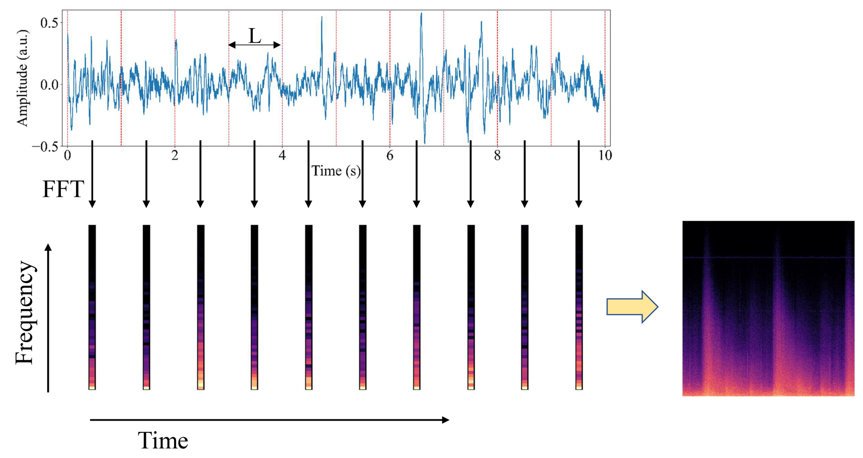
The structural health monitoring of wind turbine blades includes signal processing and fault diagnosis. As the raw signals show no significant characteristic, these signals need to be extracted before fault diagnosis [23]. Through signal processing, the features of raw signals can explore the hidden information of defects. There are some commonly used signal processing methods, such as fast Fourier transform (FFT) and short-time Fourier transform (STFT). The FFT converts time-domain signals into frequency-domain, and loses the information about time. To solve this problem, STFT is proposed to reserve the time and frequency-domain information by moving a window of fixed length on acoustic signals and applying the FFT on each segment. To distinguish the defects based on the features, it is necessary to design a fault diagnosis algorithm. With the development of deep learning, convolutional neural network (CNN) has been widely used in fault diagnosis due to the advantage of automatically extracting information without any human supervision [24]. Thus, some academics have employed CNN to achieve defect detection. Edge-side lightweight YOLOv4 [25] is proposed to achieve real-time safety management of on-site power system work. The model takes the advantages of depth-wise separable convolution and mobile inverted bottleneck convolution to reduce the size and computation of model with a high accuracy. Zhang et al. [26] used a deep convolution generative adversarial network to generate fault samples and used the residual connected convolutional neural network for feature extracting and classification. Despite the successful applications of deep learning in other fields, it still lacks in-depth research on the applications in wind turbine blade defect detection. There are still some challenges for the use of deep learning [24].

(1)

Data aspect: Defects of wind turbine blades are often repaired at an early stage, making them difficult to be obtained. In addition, the diversity of defect categories and degrees of wind turbine blades makes it hard to construct a complete dataset.

(2)

Model aspect: Common convolutional neural networks mainly have good performance on ImageNet, COCO and other datasets. The general trend has been to make deeper and more complicated networks in order to achieve higher accuracy [27], resulting in huge size and computation. Hence, these models cannot be carried out in embedded devices for edge computing. The model for WTB defect detection should be explored for actual scenarios.

(3)

Explanation aspect: Deep learning is often treated as a black box due to its complexity. Although these models enable superior performance, they lack the ability to decompose into individual intuitive components, making them difficult to interpret [28]. Therefore, it is important and meaningful to build trust in deep learning.

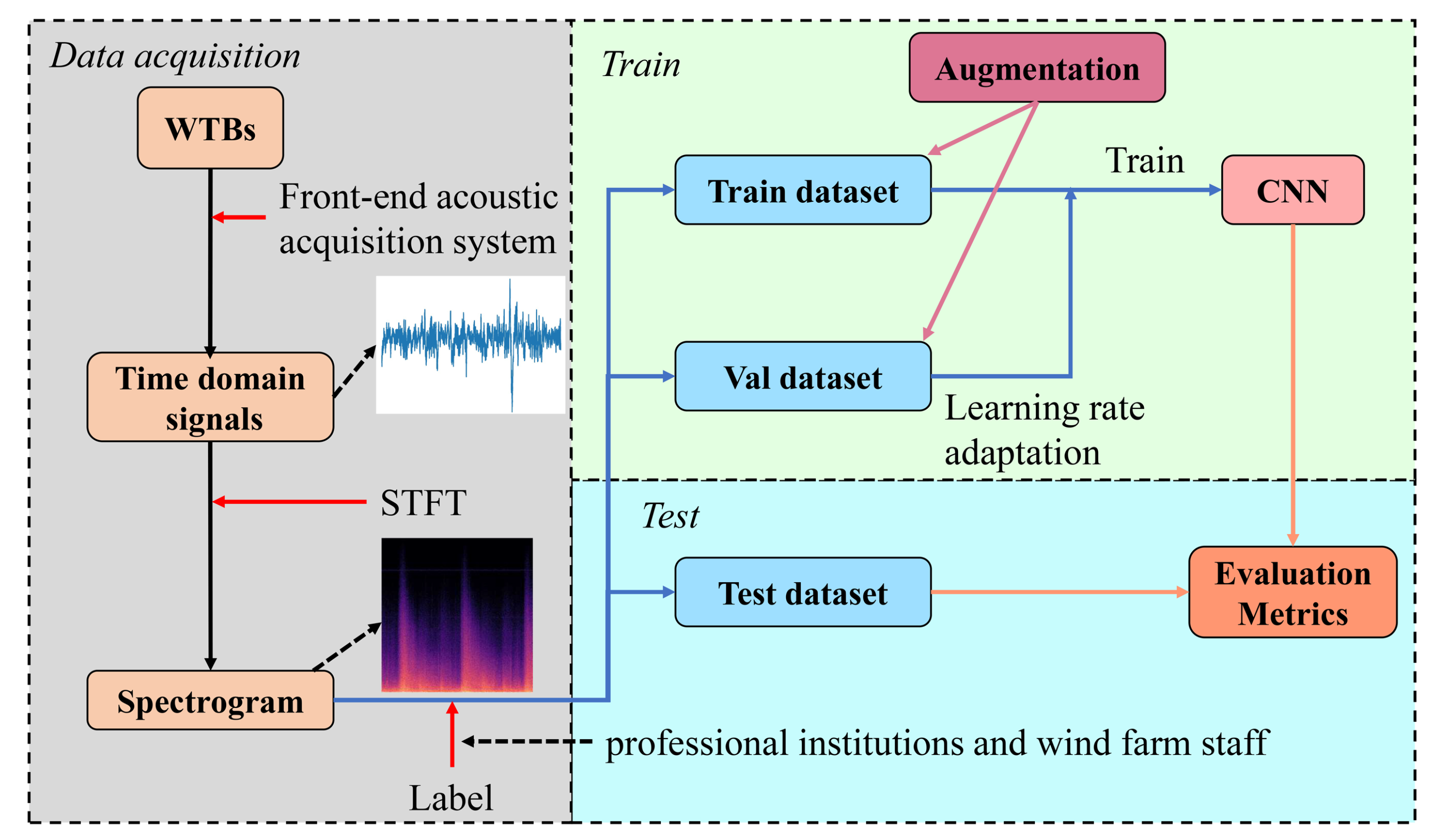
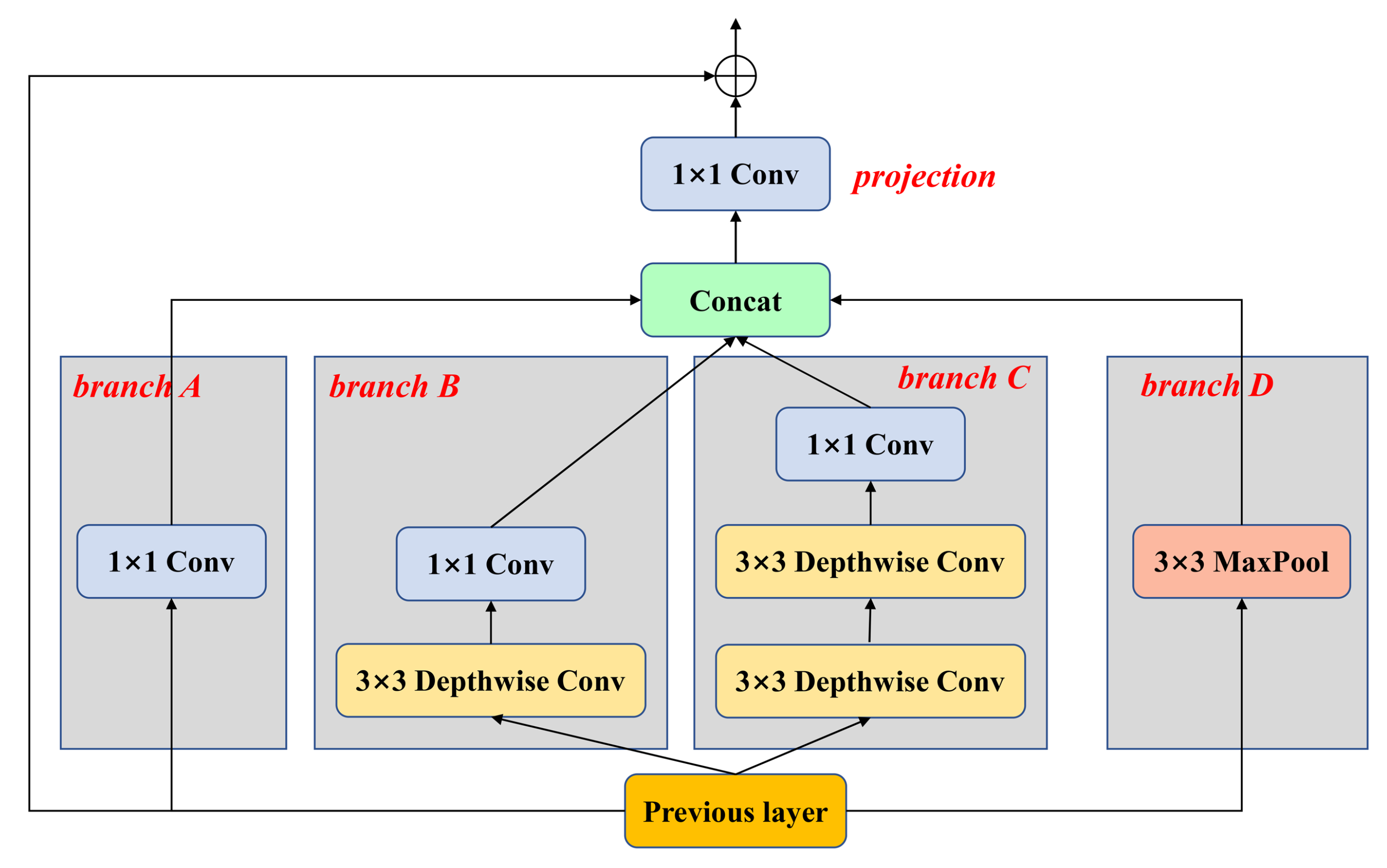
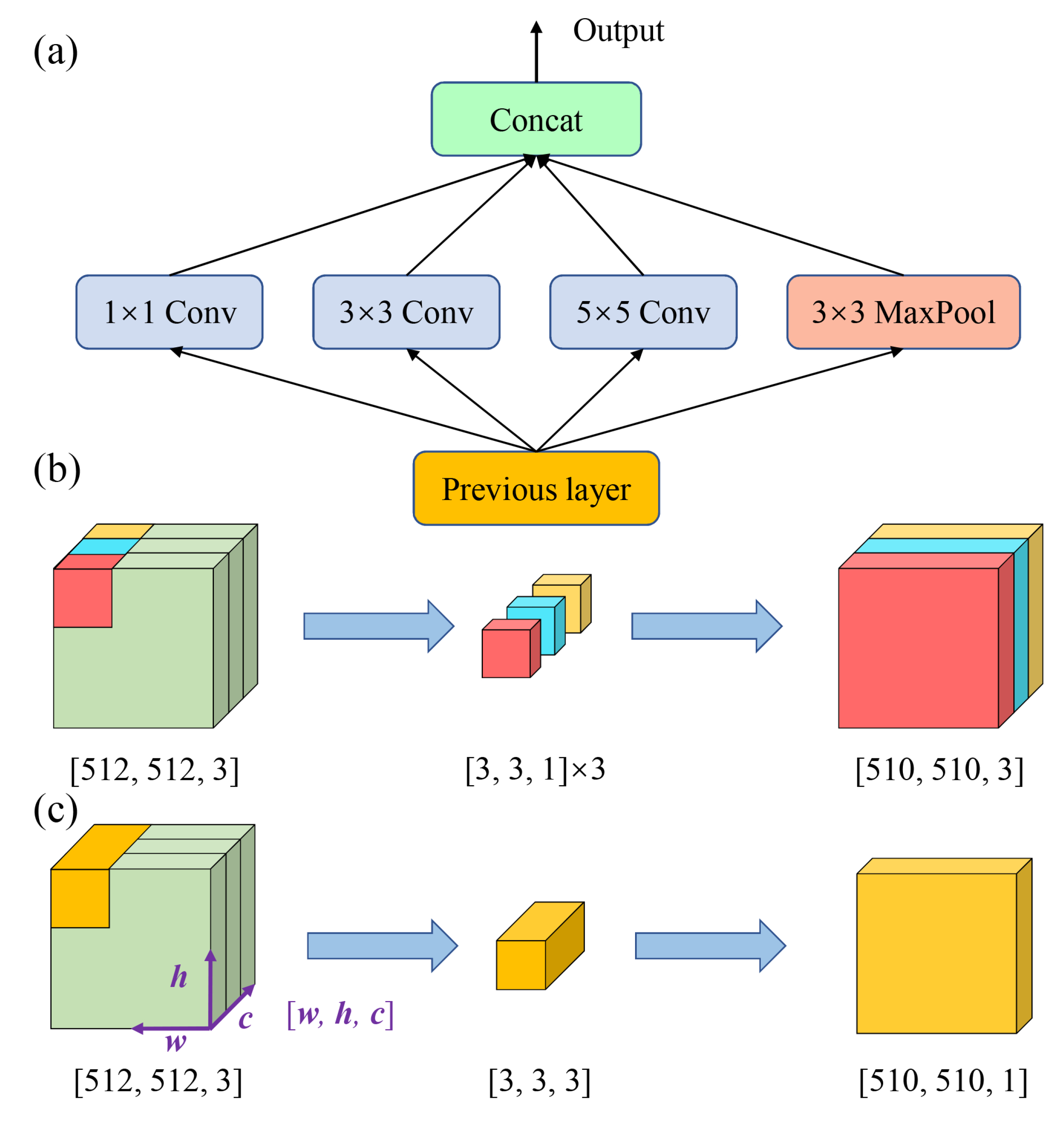
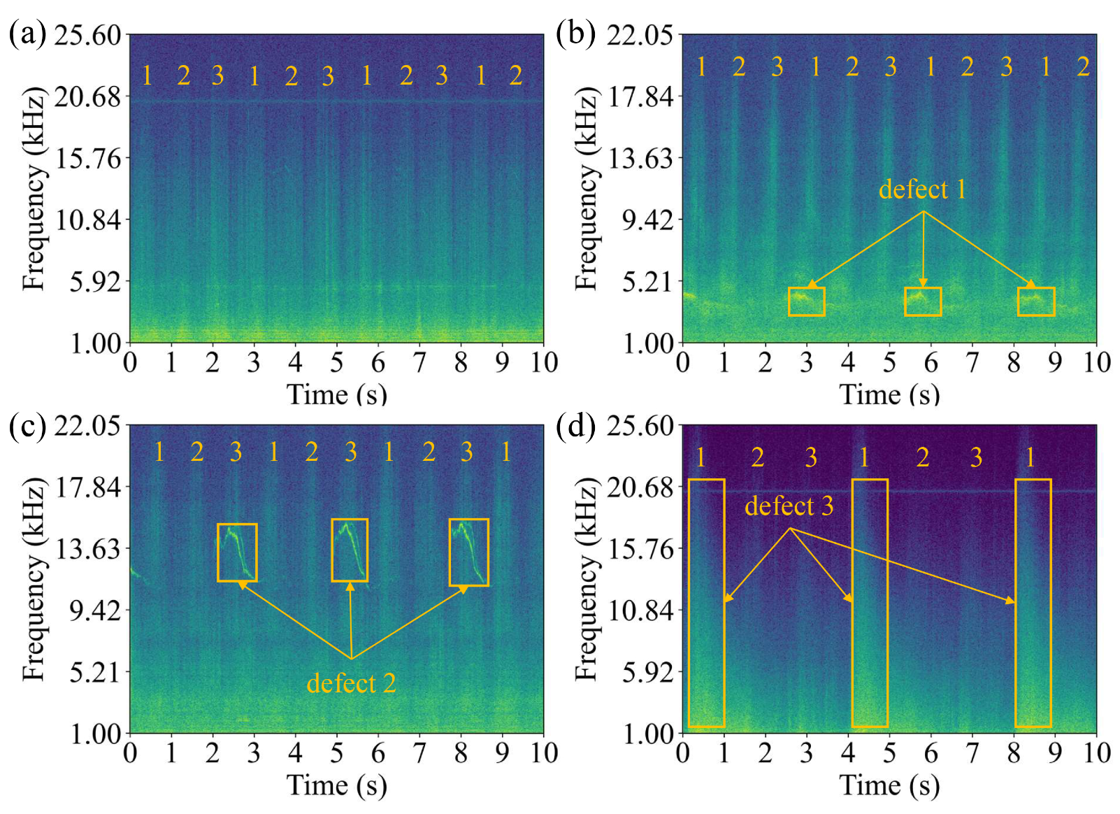
To address the above challenges, a lightweight convolutional neural network called WTBMobileNet for wind turbine blade defect detection is proposed. Specifically, for the data aspect, acoustic signals of different defect categories and degrees are collected from three wind farms (Dawu, Diaoyutai and Xiaolishan) and analyzed in detail through spectrograms. In order to alleviate the problem of data imbalance, class-balanced loss function is used in this study. For the model, WTBMobileNet is designed to implement multi-scale and efficient feature extraction, mainly combining the advantages of GoogLeNet [29], MobileNet [27] and ResNet [30]. The proposed model is compared with baseline networks in multiple aspects, which proves its effectiveness and excellent performance. In addition, the impact of different data augmentations on WTBMobileNet is analyzed, and the best-performing model is trained through four data augmentations which have positive gains. Finally, the application potential of WTBMobileNet is explored, demonstrating that the proposed model has good performance in both drone image classification and spectrogram object detection.

2. Methodology

2.1. Workflow of the Study

In order to apply CNN to wind turbine blade defect detection in embedded devices, a lightweight convolutional neural network is proposed in this paper. This approach can be outlined as in Figure 1:

(1)

Acoustic signals are collected through the front-end acoustic acquisition system and marked by professional institutions and wind farm employees.

(2)

The time-domain acoustic signals are converted into spectrograms by short-time Fourier transform, while retaining the time-domain and frequency-domain information.

(3)

Spectrograms are divided into training, validation and testing sets by a stratified sampling method, accounting for 70%, 10% and 20%, respectively.

(4)

Data augmentation is employed for the expansion of the training set and the validation set, which are used to train the model and adjust the learning rate, respectively.

(5)

The testing set is used to determine the generalization and performance of the proposed network.

2.2. Convolutional Neural Network

The convolutional neural network is the most famous and commonly network, automatically identifying relevant features without any human supervision. CNN is stacked by convolutional layers, pooling layers and fully connected layers [31]. The neurons in the convolutional layer share the same weights and bias to generate the output feature map, which are defined as a kernel or filter. The main task of the pooling layer is the down-sampling of the input feature map. The most familiar and frequently utilized pooling method is the average-pooling layer that outputs the average of the values of the sub-area. The full connected layer is located at the end of CNN and connected to all neurons of the previous layer.

2.3. Short-Time Fourier Transform

The time-domain information and frequency-domain information of acoustic signals represent the position and condition of WTBs, respectively. The Fourier transform considers the entire signal, whose frequency information is averaged, and consequently loses the information about time. Therefore, we process acoustic signals using the short-time Fourier transform (STFT) while preserving the time and frequency-domain information. STFT [32] extracts the segments of the time-domain signal by moving a window of fixed length on the time-domain signal and applying the Fourier transform on each extracted segment, hence providing time-localized frequency information in Figure 2, which can be expressed as

$$STFT(t,f)={\int }_{-\infty }^{\infty }\left[x\left(\tau \right)g(\tau -t)\right]e^{-j2\pi f\tau }d\tau$$

(1)

where x is the time-series signal, and g is the function of window.

2.4. Data Augmentation

Data augmentation is quite effective for audio to make a generalized model, which increases the size of the dataset and avoids overfitting. Data augmentation for waveform is applied to raw time-series signals, which changes how they sound. Several basic augmentation methods for waveform are as follows:

(1)

GaussianNoiseSNR: add noise that follows normal distribution, and the amplitude is decided by the Signal-to-Noise Ratio (SNR), which can be expressed as

$$\begin{array}{c}\hfill SNR=20{log}_{10}\frac{A_{\mathrm{s}}}{A_{\mathrm{n}}}\end{array}$$

(2)

where $A_{\mathrm{s}}$ and $A_{\mathrm{n}}$ are the amplitude of the signal and the noise, respectively.

(2)

PinkNoiseSNR: add noise that follows a gradual decrease in noise intensity from low frequency to high frequency, and the amplitude is determined by SNR.

(3)

PitchShift: shift the pitch of a waveform by steps, and make the sound heard as an effect higher or lower.

(4)

TimeShift: shift waveform to the left or the right with a random second.

(5)

VolumeControl: adjust the volume of the waveform.

2.5. Lightweight Module Architecture

It is very difficult to deploy a convolutional neural network in practical applications [24]. The general networks trend to be deeper and more complicated in order to achieve higher accuracy. Instead, these advances to improve accuracy are not necessarily making networks more efficient with respect to size and speed [27]. In WTB defect detection, the task needs to be carried out in a timely fashion on a computationally limited platform. Therefore, reducing the size and floating point operations (FLOPs) of networks with a high accuracy is a major problem. In this paper, a lightweight module for WTB defect detection (LW-Module) is defined which reduces computation and size with a high accuracy. The architecture of the lightweight module is shown in Figure 3.

The design of the lightweight module is based on Inception [29], shown in Figure 4a, which increases the width and depth of a model without an uncontrolled blow-up in computational complexity and abstract features at various scales. There is an inevitable increase in the number of outputs which concatenates branch A, branch B, branch C and branch D and it leads to a computational blow-up within a few stages. To solve the problem, 1 × 1 convolution, called projection, is used after the contact layer, which reduces the number of outputs. To further reduce parameters and computation, depth-wise separable convolution (DSC) [27] shown in Figure 4b is used in the module, which factorizes a standard convolution into a depth-wise convolution and a pointwise convolution. The cost of DSC and standard convolution is expressed in Equation (3). The DSC uses about $1/S_k^2$ times less computation than standard convolution at only a small reduction in accuracy. With the depth increase of the network, degradation and vanishing gradient problems have been exposed. The degradation problem is that accuracy becomes saturated and then degrades rapidly. Therefore, shortcut connections [30] are employed in the module.

$$\begin{array}{cc}\hfill COS{T}_{DSC}& =S_k*S_k*C_{in}*S_f*S_f\hfill \\ \hfill & +C_{in}*C_{out}*S_f*S_f\hfill \\ \hfill COS{T}_{conv}& =S_k*S_k*C_{in}*C_{out}*S_f*S_f\hfill \\ \hfill \frac{COS{T}_{DSC}}{COS{T}_{conv}}& =\frac{1}{C_{out}}+\frac{1}{S_k^2}\hfill \end{array}$$

(3)

where $S_k$ is the size of the kernel, $S_f$ is the size of the feature map, $C_{in}$ is the input channels, and $C_{out}$ is the output channels.

2.6. Evaluation Metrics

Wind turbine blade defect detection is treated as a classification problem, and the confusion matrix is an effective evaluation method, shown in

Table 1. The confusion matrix: 0: normal; 1: abnormal.

		Predicted
		0	1
label	0	True positive (TP)	False negation (FN)
	1	False positive (FP)	True negative (TN)

. We evaluate different networks by accuracy, precision, recall and F1-score. In this study, defect detection is a multi-class problem. Therefore, the metrics are calculated by weighted average which averages the support-weighted mean per category. Different metrics can be expressed in Equation (4). Moreover, class activation mapping (CAM) [33] is used to build a generic localizable deep representation that highlights exactly which regions of an image are important for discrimination.

$$\begin{array}{cc}\hfill accuracy& =\frac{TP+TN}{TP+FN+FP+TN}\hfill \\ \hfill precision& =\frac{TP}{TP+FP}\hfill \\ \hfill recall& =\frac{TP}{TP+FN}\hfill \\ \hfill F1-score& =2\times \frac{precision\times recall}{precision+recall}\hfill \end{array}$$

(4)

3. Empirical Analysis

3.1. Dataset

The acoustic signals are acquired by two specialized outdoor devices from three wind farms (Dawu, Diaoyutai and Xiaolishan), namely CUBE produced by 01dB and DR-60D produced by TASCAM. The technical specifications of the devices are shown in

Table 2. Technical specifications of the acquisition devices.

Specification	CUBE	DR-60D
frequency response	3.15 Hz∼20 kHz ± 2 dB	20 Hz∼20 kHz + 0.5/−2 dB
nominal sensitivity	50 mV/Pa	31.6 mV/Pa
temperature range	−40 °C∼ + 120 °C	0 °C∼ + 40 °C
sampling frequencies	51,200	44,100

. The spectrograms are extracted from acoustic signals whose length is 10 s by STFT. The dataset built by spectrograms contains a total of 4737 images. It is composed of several defects, such as crack, unbalance and others. All spectrograms are divided into four categories according to the frequency and shape of the defect information, namely Normal, Defect 1, Defect 2 and Defect 3, respectively. The spectrogram of each blade is the same for normal signals, and it is easy to be discriminated. Defect 1 is similar to Defect 2, and the defect information appears periodically. The main difference is the frequency band and shape of the defect information, as shown in Figure 5b,c. Defect 1 is a low frequency defect (below 10 kHz), and the defect information is difficult to distinguish due to the high noise. Defect 2 is a high frequency defect (above 10 kHz), and defect information is easy to distinguish. Defect 3 is special, and the spectrogram of one blade is stronger than the other two. Finally, the dataset is divided into training, validation and testing sets by a stratified sampling method, accounting for 70%, 10% and 20%, respectively.

Table 3. Details of each dataset.

Category	Training	Validation	Testing
normal	785	112	224
defect 1	555	80	159
defect 2	1224	175	350
defect 3	751	107	215
total	3315	474	948

shows the details of training, validation and testing sets.

3.2. Training WTBMobileNet

To carry out real-time WTB defect detection on the embedded device raspberry pie, we design a lightweight network based on an LW-Module, which is called WTBMobileNet. The WTBMobileNet is built on several stacked LW-Modules as mentioned in the previous section except for the first layer which is a standard convolution. The architecture of WTBMobileNet is defined in

Table 4. Architecture of WTBMobileNet.

Type	Size	Stride	Output Size	Branch Output Size
convolution	3 × 3	2	256 × 256 × 16
LW-Module		2	128 × 128 × 32	10
LW-Module		2	64 × 64 × 40	16
LW-Module		1	64 × 64 × 40	20
LW-Module		2	32 × 32 × 96	48
LW-Module		1	32 × 32 × 144	72
LW-Module		2	16 × 16 × 576	144
Avg pool	16 × 16	1	1 × 1 × 576
Linear			1 × 1 × 4

. The WTBMobileNet is stacked by a standard convolution, 6 LW-Module, average pool and a linear layer. All layers are followed by a batchnorm and LeakReLu nonlinearity function with the exception of the first standard convolution layer which is followed by a hard swish [34] and the final linear layer which has softmax nonlinearity function.

For the process of training, the spectrogram is resized into 512 × 512 taking RGB color channel with mean subtraction. The WTBMobileNet is implemented and trained in PyTorch. Adam with a batch size of 64 is used to update the model. The initial learning rate is 0.01 and the scheduler is ReduceLROnPlateau that reduces the learning rate when a metric has stopped improving, and cross entropy loss is used to estimate WTBMobileNet performance during the optimization process. For the best-performing model, the WTBMobileNet with the maximum F1-score in the validation set is saved.

The curve of error for training and validation sets is shown in Figure 6. With the increase of epoch, the errors for both training and validation sets initially decrease and finally remain stable at a large epoch. When WTBMobileNet converges, the error between both is about 0.012, which means there is no overfitting. Since the natural noise improves the robustness of acoustic signals, the overfitting effect is suppressed.

3.3. Baseline Comparison

To verify the performance of WTBMobileNet for wind turbine blade defect detection, four baseline networks are compared to WTBMobileNet. The details regarding the four baseline networks are as follows:

(1)

MobileNet is an efficient network that can be easily matched to an embedded device for vision application, and the structure is built on depth-wise separable convolutions except for the first layer which is a full convolution.

(2)

ResNet solves the degradation problem and gains accuracy from considerably increased depth. The architecture is a plain network with added shortcut connection.

(3)

VGG is a network composed of a stack of standard convolutions followed by fully connected layers. The function of the last layer is softmax.

(4)

GoogLeNet focuses on efficient architecture that improves utilization of the computing resources and has a significant quality gain compared to shallower and narrower networks.

As illustrated in

Table 5. Performance of baseline comparison on spectrogram dataset.

Model	Accuracy	Precision	Recall	F1-Score	Normal	Defect 1	Defect 2	Defect 3	FLOPs (G)	Params (M)
MobileNetV3	98.73	98.75	98.73	0.9874	98.21	98.11	98.86	99.53	1.161	2.976
ResNet34	97.89	97.94	97.89	0.9790	96.88	96.23	98.86	98.60	19.178	21.287
ResNet50	98.31	98.32	98.31	0.9830	1.00	93.08	99.14	99.07	21.47	23.516
VGG16	36.92	13.63	36.92	0.1991	0.00	0.00	1.00	0.00	80.249	14.717
VGG19	36.92	13.63	36.92	0.1991	0.00	0.00	1.00	0.00	101.999	20.026
GoogLeNet	95.46	95.52	95.46	0.9546	95.98	88.05	98.00	96.28	7.857	5.604
WTBMobileNet	97.05	97.08	97.05	0.9705	98.66	91.82	98.00	97.67	0.423	0.315

, the proposed network achieves a high accuracy with a minimum size and computation compared with the other baseline networks. The accuracy of WTBMobileNet is as high as 97.05%. In terms of precision and recall, the proposed network is above 97% for both, and the F1-score is 0.9705. The VGG16 and VGG19 [35] have bad performance for health monitoring of wind turbine blades. The predictions of both for all spectrograms in the testing set are Defect 2, which means the networks cannot distinguish different categories. This implies the stacked standard convolution may not be able to fully mine the discriminative features from spectrograms for wind turbine blades. Compared with the worst-performing model (GoogLeNet), WTBMobileNet is about 17.8 times smaller with 18.6 times less computation. The proposed network is 1.59% more accurate than GoogLeNet, and there is an improvement of 1.56% and 1.59% with regards to precision and recall, respectively. The best-performance model is the MobileNetV3 [34], which is 1.68% more accurate than the proposed method. However, WTBMobileNet is about 9.4 times smaller with 2.7 times less computation. In addition, the performance of WTBMobileNet can be improved to the same level when using data augmentation. Overall, WTBMobileNet has good performance in wind turbine blade health monitoring and has potential for practical applications.

3.4. WTBMobileNet Result

The result of WTBMobileNet is displayed in a confusion matrix, as shown in Figure 7a, where the x-axis is label type and the y-axis is predicted type. The WTBMobileNet without augmentation can accurately distinguish most spectrograms in the testing set, and only 28 samples are incorrectly identified. The proposed network exhibited the accuracy of 97.05%, precision of 97.08%, recall of 97.05% and F1-score of 0.9705. This means that WTBMobileNet has a good performance in wind turbine blade health monitoring. However, the proposed model is not good at identifying Defect 1 with an accuracy of only 91.82% compared to 98.11% for MobileNetV3. This indicates that Defect 1 can theoretically be identified accurately, and WTBMobileNet still has potential for improvement.

To improve the performance of WTBMobileNet, a data augmentation analysis is performed. The results are presented in

Table 6. Augmentation comparison on spectrogram dataset. (The model of A∼G is WTBMobileNet.)

Augmentation	A	B	C	D	E	F	G
GaussianNoiseSNR		✓					✓
PinkNoiseSNR			✓				✓
PitchShift				✓			✓
TimeShift					✓		✓
VolumeControl						✓
accuracy	97.05	98.10	97.89	97.15	98.10	96.73	98.10
change		1.05	0.84	0.10	1.05	−0.32	1.05

and

Table 7. Performance of WTBMobileNet on different augmentation.

Model	Accuracy	Precision	Recall	F1-Score	Normal	Defect 1	Defect 2	Defect 3
A	97.05	97.08	97.05	0.9705	98.66	91.82	98.00	97.67
B	98.10	98.12	98.10	0.9810	96.88	96.23	99.43	98.60
C	97.89	97.91	97.89	0.9789	97.32	95.60	98.86	98.60
D	97.15	97.18	97.15	0.9714	98.21	91.82	98.00	98.60
E	98.10	98.17	98.10	0.9812	97.32	96.23	98.86	99.07
F	96.73	96.82	96.73	0.9674	94.20	98.11	99.14	94.42
G	98.10	98.14	98.10	0.9811	98.21	95.60	99.14	98.14

. The five data augmentations mentioned in the previous section are used to improve the performance of WTBMobileNet. All augmentations except VolumeControl have positive gains. The accuracy improvement of model B, C, D, E and F are 1.05%, 0.84%, 0.1%, 1.05% and −0.32%, respectively. As illustrated in Table 7, GaussianNoiseSNR, PinkNoiseSNR, TimeShift and VolumeControl significantly improve the ability to identify Defect 1, which is 4.41%, 3.78%, 4.41% and 6.29%, respectively. Therefore, WTBMobileNet, called model G in Table 6 is trained through four data augmentations which have positive gains. Compared with model A (WTBMobileNet without data augmentation), model G has 1.05%, 1.06% and 1.05% improvements in accuracy, precision and recall, respectively. Moreover, model G significantly improves the accuracy of Defect 1, from 91.82% to 95.6%. The confusion matrix of model G is shown in Figure 7b. The number of misclassified spectrograms decreases from 28 to 18, and most of them are misidentified as Defect 3. Further, all misclassified spectrograms are analyzed. Some of them contain multiple defects at the same time, with the manually marked defects being more pronounced. It is difficult to solve this problem by classification, so we try object detection to deal with the problem in a later section.

3.5. Visual Explanation

Networks based on convolution have unprecedented breakthroughs in vision application but are often considered as black boxes because of their explanation and transparency [28]. Networks should not only be accurate, but also interpretable, especially when providing incorrect predictions. Thus, interpretability is the key factor in this study. This makes the networks not only more credible, but also more reliably deployable.

Class activation mapping showing the attention of networks is used to visually explain the results of WTBMobileNet to make it more explainable and transparent. Figure 8 indicates the visual explanation of four categories. For normal spectrograms, WTBMobileNet pays attention to two frequency bands (1 kHz∼6 kHz and 13 kHz∼22 kHz), especially the low frequency. This is in line with our expectation, since defects are mainly in these two frequency bands. Regarding Defect 1 and Defect 2, the network focuses on the corresponding defect information, respectively, as shown in Figure 8b,c. For Defect 3, the network mainly focuses on the spectrogram of one blade which is stronger than the other two. The CAM results for different categories show that WTBMobileNet accurately focuses on the defect information of four categories, has good interpretability, and achieves reliable deployment.

4. Discussion

4.1. Application for Image Classification

Visual inspection is also an important technique commonly used to find faults in WTBs. In this section, a binary classification image dataset from drones inspection is built. The image dataset has a total of 9235 images and is divided into training, validation and testing sets in the same way as the spectrogram dataset. The detail of the the image dataset is shown in

Table 8. Detail of each dataset on images.

Set	Normal	Abnormal	Total
training	4502	1962	6464
validation	643	281	924
testing	1286	561	1847

. The performance of WTBMobileNet on the image dataset is explored, comparing it to different baseline networks, as illustrated in

Table 9. Performance of baseline comparison on image dataset.

Model	Accuracy	Precision	Recall	F1-Score	Normal	Abnormal
MobileNetV3	86.68	88.63	88.68	0.8865	92.30	88.39
ResNet34	88.63	88.79	88.63	0.8870	90.90	0.83
ResNet50	85.33	85.98	85.33	0.8554	86.94	81.64
VGG16	69.63	48.48	69.63	0.5716	1.00	0.00
VGG19	69.63	48.48	69.63	0.5716	1.00	0.00
GoogLeNet	91.07	90.98	91.07	0.9095	95.41	81.11
WTBMobileNet	89.55	89.71	89.55	0.8961	91.52	85.03

. The proposed network is the second-performing model with just 1.52% lower accuracy than the best-performing model (GoogLeNet). However, WTBMobileNet is about 17.8 times smaller with 18.6 times less computation. In addition, the accuracy is 5.87%, 0.7% and 0.92% higher than MobileNetV3, ResNet34 and ResNet50, respectively. As a result, WTBMobileNet reduces the size and computation with only a small decrease in accuracy and has the potential for drone inspection of wind turbine blades.

4.2. Application for Object Detection

In practice, wind turbine blades usually have a variety of defects at the same time, so classification is difficult to use to solve the problem. Hence, Faster R-CNN [36] based on WTBMobileNet is proposed to solve this problem. Mean average precision (mAP) for different Intersection-over-Union (IOU) is used to evaluate the performance of the model. The result of mAP@0.5, mAP@0.75 and mAP@[0.5, 0.95] are 96.4%, 73.6% and 70.7%, respectively. Figure 9 shows some results on the spectrograms in the testing set. The red is the ground-truth box, and the yellow is the predicted box. The Faster R-CNN based on WTBMobileNet can identify and locate defects in the spectrograms well and achieve multi-defect detection. Although some defects are not detected, this can be improved by optimizing the model.

5. Conclusions

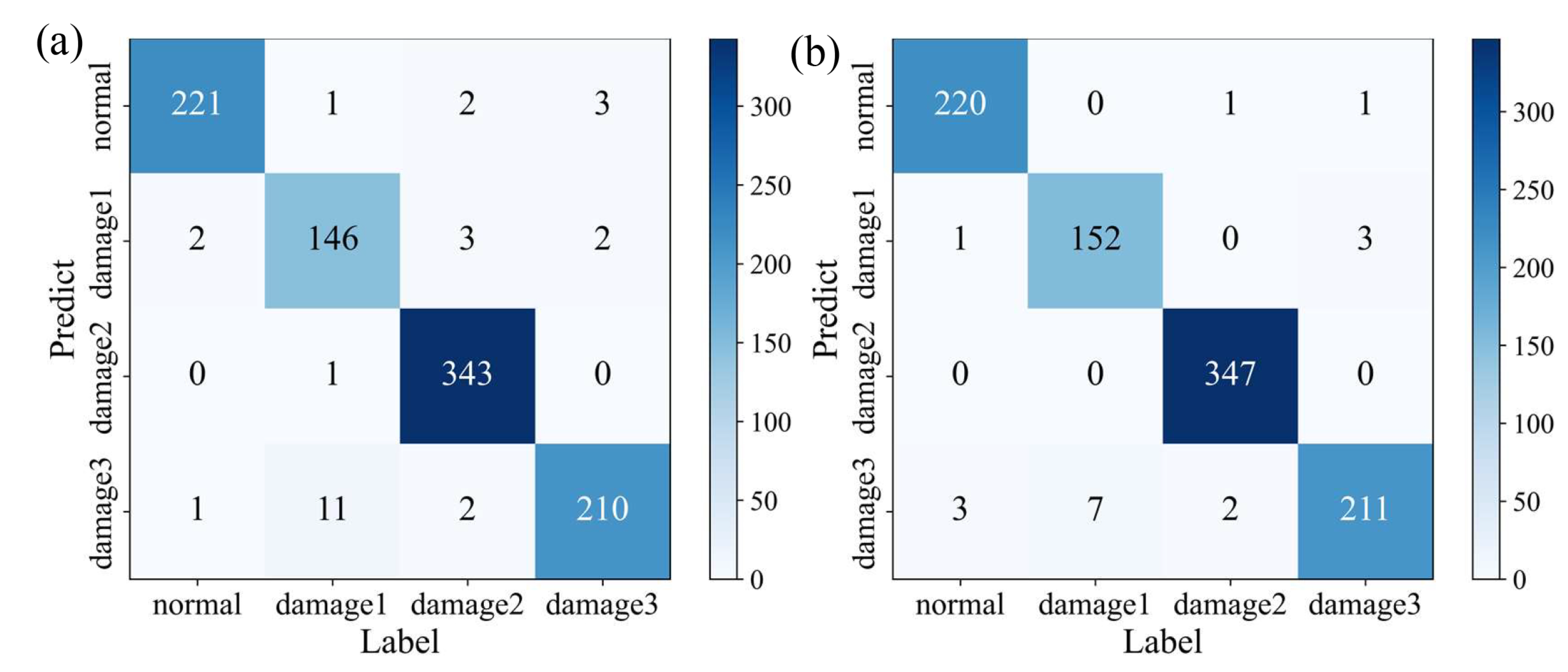
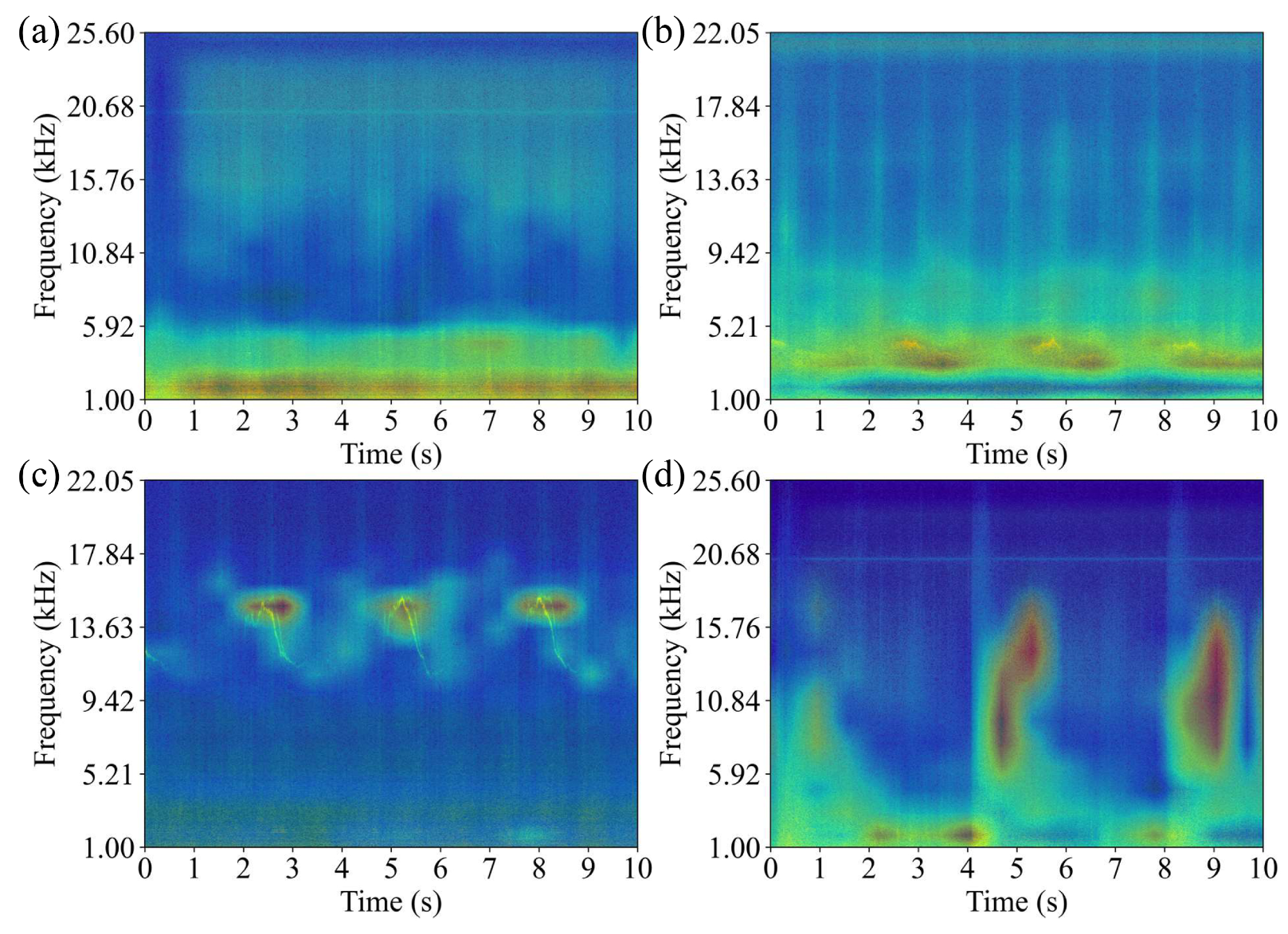
In this paper, to address the challenges of deep learning, a lightweight convolutional neural network is proposed for the embedded devices, which reduces size and FLOPs with a small decrease in accuracy, to implement wind turbine blade defect detection. Compared with the baseline models, the proposed model has an accuracy of 95.6%, and the amount of parameters and computation are 0.315 million and 0.423 GFLOPs, respectively. To further improve the performance of WTBMobileNet, five data augmentations are analyzed, where GaussianNoiseSNR, PinkNoiseSNR, PitchShift and TimeShift have positive gains. The WTBMobileNet with four data augmentations has an accuracy of 98.1%, and improves the accuracy of Defect 1 from 91.82% to 95.6%. In addition, the interpretability and transparency of WTBMobileNet are demonstrated through CAM. Finally, WTBMobileNet is tested in drone image classification and spectrogram object detection. The accuracy, mAP@0.5, mAP@0.75 and mAP@[0.5, 0.95], is 89.55% and 96.4% and 73.6% and 70.7%, respectively, proving that WTBMobileNet has great potential in these two applications.

In the future, we would like to further study the deep-learning-based defect detection method for wind turbine blades from two aspects. First, we would like to optimize the Faster R-CNN to achieve multi-scale and high-accuracy object detection in drone inspection. Second, we would like to combine acoustics and vision to achieve multimodal defect detection for wind turbine blades.

References

1. Du, Y.; Zhou, S.; Jing, X.; Peng, Y.; Wu, H.; Kwok, N. Damage detection techniques for wind turbine blades: A review. Mech. Syst. Signal Process. 2020, 141, 106445. [Google Scholar]
2. Gao, Z.; Liu, X. An overview on fault diagnosis, prognosis and resilient control for wind turbine systems. Processes 2021, 9, 300. [Google Scholar] [CrossRef]
3. Jin, X.; Chen, Y.; Wang, L.; Han, H.; Chen, P. Failure prediction, monitoring and diagnosis methods for slewing bearings of large-scale wind turbine: A review. Measurement 2021, 172, 108855. [Google Scholar] [CrossRef]
4. Ren, Z.; Verma, A.S.; Li, Y.; Teuwen, J.J.E.; Jiang, Z. Offshore wind turbine operations and maintenance: A state-of-the-art review. Renew. Sustain. Energy Rev. 2021, 144, 110886. [Google Scholar]
5. Tian, W.; Cheng, X.; Li, G.; Shi, F.; Chen, S.; Zhang, H. A multilevel convolutional recurrent neural network for blade icing detection of wind turbine. IEEE Sens. J. 2021, 21, 20311–20323. [Google Scholar] [CrossRef]
6. Attallah, O.; Ibrahim, R.A.; Zakzouk, N.E. Fault diagnosis for induction generator-based wind turbine using ensemble deep learning techniques. Energy Rep. 2022, 8, 12787–12798. [Google Scholar] [CrossRef]
7. Jia, X.; Han, Y.; Li, Y.; Sang, Y.; Zhang, G. Condition monitoring and performance forecasting of wind turbines based on denoising autoencoder and novel convolutional neural networks. Energy Rep. 2021, 7, 6354–6365. [Google Scholar] [CrossRef]
8. Tummala, A.; Velamati, R.K.; Sinha, D.K.; Indraja, V.; Krishna, V.H. A review on small scale wind turbines. Renew. Sustain. Energy Rev. 2016, 56, 1351–1371. [Google Scholar]
9. Porté-Agel, F.; Bastankhah, M.; Shamsoddin, S. Wind-turbine and wind-farm flows: A review. Bound. Layer Meteorol. 2020, 174, 1–59. [Google Scholar]
10. Ciuriuc, A.; Rapha, J.I.; Guanche, R.; Domínguez-García, J.L. Digital tools for floating offshore wind turbines (FOWT): A state of the art. Energy Rep. 2022, 8, 1207–1228. [Google Scholar] [CrossRef]
11. Li, D.; Ho, S.C.M.; Song, G.; Ren, L.; Li, H. A review of damage detection methods for wind turbine blades. Smart Mater. Struct. 2015, 24, 033001. [Google Scholar] [CrossRef]
12. Civera, M.; Surace, C. Non-destructive techniques for the condition and structural health monitoring of wind turbines: A literature review of the last 20 years. Sensors 2022, 22, 1627. [Google Scholar] [CrossRef] [PubMed]
13. Effiom, S.O.; Nwankwojike, B.N.; Abam, F.I. Economic cost evaluation on the viability of offshore wind turbine farms in Nigeria. Energy Rep. 2016, 2, 48–53. [Google Scholar] [CrossRef] [Green Version]
14. García Márquez, F.P.; Peco Chacón, A.M. A review of non-destructive testing on wind turbines blades. Renew. Energy 2020, 161, 998–1010. [Google Scholar] [CrossRef]
15. Bebars, A.D.; Eladl, A.A.; Abdulsalam, G.M.; Badran, E.A. Internal electrical fault detection techniques in DFIG-based wind turbines: A review. Prot. Control Mod. Power Syst. 2022, 7, 18. [Google Scholar] [CrossRef]
16. Song, X.; Xing, Z.; Jia, Y.; Song, X.; Cai, C.; Zhang, Y.; Wang, Z.; Guo, J.; Li, Q. Review on the damage and fault diagnosis of wind turbine blades in the germination stage. Energies 2022, 15, 7492. [Google Scholar] [CrossRef]
17. Zhang, Y.; Avallone, F.; Watson, S. Wind turbine blade trailing edge crack detection based on airfoil aerodynamic noise: An experimental study. Appl. Acoust. 2022, 191, 108668. [Google Scholar] [CrossRef]
18. Wang, M.H.; Lu, S.D.; Hsieh, C.C.; Hung, C.C. Fault detection of wind turbine blades using multi-channel CNN. Sustainability 2022, 14, 1781. [Google Scholar] [CrossRef]
19. Wang, X.; Liu, Z.; Zhang, L.; Heath, W.P. Wavelet package energy transmissibility function and its application to wind turbine blade fault detection. IEEE Trans. Ind. Electron. 2022, 69, 13597–13606. [Google Scholar] [CrossRef]
20. Sreeraj, K.; Maheshwari, H.K.; Rajagopal, P.; Ramkumar, P. Non-contact monitoring and evaluation of subsurface white etching area (WEA) formation in bearing steel using Rayleigh surface waves. Tribol. Int. 2021, 162, 107134. [Google Scholar] [CrossRef]
21. Tsai, T.C.; Wang, C.N. Acoustic-based method for identifying surface damage to wind turbine blades by using a convolutional neural network. Meas. Sci. Technol. 2022, 33, 085601. [Google Scholar] [CrossRef]
22. Reddy, A.; Indragandhi, V.; Ravi, L.; Subramaniyaswamy, V. Detection of Cracks and damage in wind turbine blades using artificial intelligence-based image analytics. Measurement 2019, 147, 106823. [Google Scholar] [CrossRef]
23. Tang, Z.; Wang, M.; Ouyang, T.; Che, F. A wind turbine bearing fault diagnosis method based on fused depth features in time-frequency-domain. Energy Rep. 2022, 8, 12727–12739. [Google Scholar] [CrossRef]
24. Alzubaidi, L.; Zhang, J.; Humaidi, A.J.; Al-Dujaili, A.; Duan, Y.; Al-Shamma, O.; Santamaría, J.; Fadhel, M.A.; Al-Amidie, M.; Farhan, L. Review of deep learning: Concepts, CNN architectures, challenges, applications, future directions. J. Big Data 2021, 8, 53. [Google Scholar]
25. Li, Q.; Zhao, F.; Xu, Z.; Li, K.; Wang, J.; Liu, H.; Qin, L.; Liu, K. Improved YOLOv4 algorithm for safety management of on-site power system work. Energy Rep. 2022, 8, 739–746. [Google Scholar] [CrossRef]
26. Zhang, D.; Ning, Z.; Yang, B.; Wang, T.; Ma, Y. Fault diagnosis of permanent magnet motor based on DCGAN-RCCNN. Energy Rep. 2022, 8, 616–626. [Google Scholar] [CrossRef]
27. Howard, A.G.; Zhu, M.; Chen, B.; Kalenichenko, D.; Wang, W.; Weyand, T.; Andreetto, M.; Adam, H. MobileNets: Efficient Convolutional Neural Networks for Mobile Vision Applications. arXiv 2017, arXiv:1704.04861. [Google Scholar]
28. Selvaraju, R.R.; Cogswell, M.; Das, A.; Vedantam, R.; Parikh, D.; Batra, D. Grad-CAM: Visual explanations from deep networks via gradient-based localization. Int. J. Comput. Vis. 2020, 128, 336–359. [Google Scholar] [CrossRef] [Green Version]
29. Szegedy, C.; Liu, W.; Jia, Y.; Sermanet, P.; Reed, S.; Anguelov, D.; Erhan, D.; Vanhoucke, V.; Rabinovich, A. Going deeper with convolutions. In Proceedings of the 2015 IEEE Conference on Computer Vision and Pattern Recognition (CVPR), Boston, MA, USA, 7–12 June 2015. [Google Scholar]
30. He, K.; Zhang, X.; Ren, S.; Sun, J. Deep residual learning for image recognition. In Proceedings of the 2016 IEEE Conference on Computer Vision and Pattern Recognition (CVPR), Las Vegas, NV, USA, 27–30 June 2016. [Google Scholar]
31. Huang, K.; Liu, X.; Fu, S.; Guo, D.; Xu, M. A Lightweight Privacy-Preserving CNN Feature Extraction Framework for Mobile Sensing. IEEE Trans. Dependable Secur. Comput. 2021, 18, 1441–1455. [Google Scholar] [CrossRef]
32. Ali, O.; Saif-Ur-Rehman, M.; Dyck, S.; Glasmachers, T.; Iossifidis, I.; Klaes, C. Enhancing the decoding accuracy of EEG signals by the introduction of anchored-STFT and adversarial data augmentation method. Sci. Rep. 2022, 12, 4245. [Google Scholar] [PubMed]
33. Zhou, B.; Khosla, A.; Lapedriza, A.; Oliva, A.; Torralba, A. Learning deep features for discriminative localization. In Proceedings of the 2016 IEEE Conference on Computer Vision and Pattern Recognition (CVPR), Las Vegas, NV, USA, 27–30 June 2016. [Google Scholar]
34. Howard, A.; Sandler, M.; Chen, B.; Wang, W.; Chen, L.C.; Tan, M.; Chu, G.; Vasudevan, V.; Zhu, Y.; Pang, R.; et al. Searching for MobileNetV3. In Proceedings of the 2019 IEEE/CVF International Conference on Computer Vision (ICCV), Seoul, Republic of Korea, 27 October–2 November 2019. [Google Scholar]
35. Simonyan, K.; Zisserman, A. Very deep convolutional networks for large-scale image recognition. arXiv 2014, arXiv:1409.1556. [Google Scholar]
36. Ren, S.; He, K.; Girshick, R.; Sun, J. Faster R-CNN: Towards real-time object detection with region proposal networks. IEEE Trans. Pattern Anal. Mach. Intell. 2017, 39, 1137–1149. [Google Scholar] [CrossRef] [PubMed]
Figure 1. The framework of wind turbine blade defect detection based on CNN.
Machines 11 00099 g001
Figure 2. The diagram of short-time Fourier transform.
Machines 11 00099 g002
Figure 3. Principle and structure diagram of lightweight module.
Machines 11 00099 g003
Figure 4. Schematic of: (a) inception; (b) depth-wise convolution; (c) standard convolution.
Machines 11 00099 g004
Figure 5. The spectrogram of (a) normal (CUBE, Dawu); (b) Defect 1 (DR-60D, Dawu); (c) Defect 2 (DR-60D, Dawu); and (d) Defect 3 (CUBE, Diaoyutai).
Machines 11 00099 g005
Figure 6. The error of WTBMobileNet with the epochs increasing.
Machines 11 00099 g006
Figure 7. Confusion matrix of WTBMobileNet: (a) without data augmentation; (b) with data augmentation.
Machines 11 00099 g007
Figure 8. Class activation mapping for: (a) Normal (CUBE, Dawu); (b) Defect 1 (DR-60D, Dawu); (c) Defect 2 (DR-60D, Dawu); and (d) Defect 3 (CUBE, Diaoyutai).
Machines 11 00099 g008
Figure 9. Examples of object detection results on the spectrograms using the Faster R-CNN based on WTBMobileNet. The red is the ground-truth box, and the yellow is the predicted box.
Machines 11 00099 g009