Article

Active Braking Strategy Considering VRU Motion States in Curved Road Conditions

School of Automotive and Traffic Engineering, Jiangsu University, Zhenjiang 212013, China
*
Author to whom correspondence should be addressed.
Machines 2023, 11(1), 100; https://doi.org/10.3390/machines11010100
Submission received: 22 November 2022 / Revised: 29 December 2022 / Accepted: 30 December 2022 / Published: 11 January 2023
(This article belongs to the Section Vehicle Engineering)

Abstract

:
Currently, the active braking system is primarily used to avoid collisions between vehicles and vulnerable road users (VRUs) traversing the road at a constant speed in straight road conditions. Research on the collision avoidance strategy has been conducted to enhance the protective effects of the active braking system for VRUs traversing the road in various motion states in curved road conditions. Firstly, the spatial position relationships between VRUs and turn-taking vehicles are established when VRUs traverse the road in various motion states from the outside or the inside of the curved road; a mathematical model is established to identify whether VRUs are in a dangerous condition. Secondly, the safe distance model is established to formulate the vehicle collision avoidance strategy. Thirdly, the active braking controller is designed based on the upper sliding mode control and the lower discrete PID control. Finally, the six collision test scenarios on the curved road are constructed by utilizing the Prescan and Matlab/Simulink software. The results show that the active braking system can avoid the collision between the vehicle and VRUs traversing the curved road in various motion states.

1. Introduction

In 2022, the Global Road Safety Report released by the World Health Organization pointed out that approximately 1.3 million people die in road traffic accidents every year, and the loss caused by road traffic accounts for 3% of the gross domestic product of most countries. More than half of all road traffic accident fatalities were vulnerable road users (VRUs). According to statistics from the United States Centers for Disease Control and Prevention, over 10,000 VRUs die, and about 300,000 VRUs are injured in road traffic accidents in the United States every year.
In China, VRU fatalities account for 70% of road traffic fatalities, including 40% for two-wheeled and 25% for pedestrians [1]. Most two-wheeled cyclists are electric bicycle riders. Currently, there are as many as 300 million electric bicycles in China. National Mandatory Standard “Safety Technical Specifications for Electric Bicycles” (GB17761-2018) states that the maximum speed of electric bicycles, as well as the quality of the vehicle as a whole, must be less than 20 km/h and 55 kg. However, due to the low awareness of safety among people, the speed modification of electric bikes is widespread, and the maximum speed is as much as 30 to 40 km/h. The vast majority of electric bicycle riders are not professionally trained and have poor safety protective equipment leading to the frequent occurrence of electric bicycle accidents, resulting in enormous loss of life and property [2]. According to the annual report of China’s traffic accident statistics, from 2015 through 2020, the death toll of electric bicycle riders increased year by year, with an increased rate of 35.2% and an average annual growth rate of 5.1% [3].
Naci et al. pointed out that each year, over 180,000 electric bicycle riders were killed in road traffic accidents, most of which occur in middle-income countries [4]. Guo et al. found that drivers’ distracted driving and irregular driving behaviors were two of the main reasons for road traffic accidents [5]. Rosén et al. studied the relationship between the speed of vehicle collisions and VRU fatality rate, pointing out that when the collision speed of the vehicle was decreased from 50 km/h to 40 km/h, the VRU fatality rate was reduced by a factor of two. A reduction in vehicle collision speed from 50 km/h to 30 km/h resulted in a five-fold reduction in the VRU fatality rate [6]. Zhao et al. [7] and Edwards et al. [8] showed that an active braking system can assist and replace the driver to implement braking, effectively avoiding collision between the vehicle and VRUs. Themann et al. [9] and Bachmann et al. [10] pointed out that the position of VRUs could be accurately obtained by using the communication technology between vehicles and infrastructure as well as the communication technology based on smartphones or smartwatches, in order to enhance the collision avoidance effect of the active braking system. Nkenyereye et al. found that VRU positions and motion information could be quickly transmitted based on 5G communication technology [11]. As a result, the decision time of the active braking system was significantly improved. Eilbrecht et al. used a neural network algorithm to identify the motion intention of VRUs, and the optimal active braking control of automobiles was achieved based on mixed-integer programming and model prediction (MPC) [12]. Park et al. proposed an active braking system based on the funnel algorithm, which accurately calculated the collision probability between the vehicle and VRUs as well as the safe distance of active braking based on the current position and expected position of the VRUs [13]. Guo et al. studied the active braking controller based on the upper sliding mode control and the lower single neuron PID control, which could be applied to flat deceleration or emergency braking conditions [14]. Li et al. proposed a human–vehicle co-driving control system based on deep learning to effectively avoid the collision between the vehicle and VRUs and designed a depth-enhanced Q network algorithm to shorten the learning time for the optimal braking strategy [15]. Lee et al. proposed a pedestrian motion trajectory prediction method based on multi-sensor fusion to improve the prediction accuracy and formulate an accurate active braking control strategy [16]. Zadeh et al. studied the collision warning system based on the geometric method; considering the age of the drivers and pedestrians, the vehicle acceleration, the weather conditions, and other factors, the corresponding active braking control strategy was proposed [17]. Duan et al. analyzed the driver’s braking behavior during the collision between the vehicle and the two-wheeled vehicle. An adaptive braking control strategy based on the driver’s braking behavior was proposed, which can activate the active braking system without interfering with the driver’s normal driving and effectively avoid the collision between the car and the two-wheeled vehicle. [18]. Peng et al. investigated the design parameters that influence the protective effect of the active braking system on two-wheeled bicycle riders; targeting the effect of collision avoidance, technical cost, and occupant comfort, multi-objective optimization research of the active braking system was performed [19].
Pan designed the VRU trajectory prediction algorithm based on the deep learning model, and a significant improvement in prediction accuracy was observed compared to the Kalman filtering algorithm, which was useful in achieving the anticipated deceleration, satisfying both safety and ride comfort [20]. Wang et al. proposed an active braking system control strategy based on the vehicular Internet of Things; since the vehicle-to-vehicle communication technology was used to obtain the motion information of VRUs to determine the danger level of VRUs and to establish a hierarchical braking strategy, the safety of VRUs was significantly improved [21]. Li proposed the pedestrian collision avoidance method based on the hierarchical conflict space, which achieves smooth vehicle braking based on the premise of meeting vehicle collision avoidance requirements; due to the negative impact that communication delay has on pedestrian collision avoidance systems, in order to improve the real-time performance of pedestrian information, a pedestrian motion estimation method was proposed that achieves safe collision avoidance [22]. Yuan et al. recognized pedestrian motion features based on a convolutional neural network and judged pedestrians’ subjective intentions; the Kalman filter algorithm was used to obtain the predicted trajectory that is consistent with the subjective intent of pedestrians, to design the active braking control algorithm, which can ensure the smoothness of the braking deceleration process and the smoothness of traffic flow [23].
The above active braking system studies are primarily concerned with assessing the safety of VRUs traversing the road at a constant speed under straight road conditions to determine whether VRUs are at risk; active braking is used to prevent collision between the vehicle and VRUs. However, on one hand, due to the complexity of the road environment, vehicles often drive on curved roads [24,25] and it is difficult to comprehensively measure the collision avoidance effect of the active braking system based on straight road conditions; On the other hand, the movement state of VRUs when crossing the road presents diversity, and they often traverse the road with uniform speed, uniform acceleration, and uniform deceleration. Therefore, given the limitations of previous studies, this paper proposes the collision avoidance strategy of the active braking system when vulnerable road users traverse the road in various motion states under curved road conditions. To test the protective effect of the active braking system, an electric bicycle rider is taken as the specific research object.

2. The Position of the Vehicle and VRUs under Curved Road Conditions

Under curved road conditions, it is necessary to identify the position of VRUs to effectively avoid collision between the vehicle and VRUs. When a VRU crosses the road from the outside to the inside of the curve, the motion diagram of the vehicle and VRU is shown in Figure 1a. In Figure 1a, C is the center of mass of the VRU; V ego is the vehicle’s driving speed; V is the movement speed of the VRU; A 1 B 1 is the driving trajectory of the vehicle; C 1 D 1 is the motion trajectory of the VRU; M 1 is the intersection of two trajectories; the millimeter-wave radar is installed at the vehicle bumper level, and oxy is the coordinate system of the millimeter-wave radar installation; ρ 1 is the distance from the vehicle to the VRU obtained from the millimeter-wave radar detection; θ 1 is the angle between the vehicle and the VRU obtained from the millimeter-wave radar detection; O is the curvature center of the curve; R is the radius of curvature of the vehicle’s driving path; and α 1 is the angle between the curvature radius of the vehicle’s driving trajectory and the motion path of the VRU.
The curvature radius of the vehicle driving trajectory R is:
R = V ego W ego
The angle between the curvature radius of the vehicle’s driving trajectory and the motion path of the VRU α 1 is:
α 1 = arctan ρ 1 cos θ 1 R + ρ 1 sin θ 1
The lateral distance of the VRU relative to the vehicle y 1 is:
y 1 = R 2 + 2 ρ 1 R sin θ 1 + ρ 1 2 R
The trajectory length of the vehicle driving to point M 1 , x 1 is:
x 1 = R α 1
When a VRU crosses the road from the inside to the outside of the curve, the motion diagram of the vehicle and VRU is shown in Figure 1b. In this figure, A 2 B 2 is the driving trajectory of the vehicle; C 2 D 2 is the motion trajectory of the VRU; M 2 is the intersection of the two trajectories; the millimeter-wave radar is installed at the vehicle bumper level, and oxy is the coordinate system of the millimeter-wave radar installation; ρ 2 is the distance from the vehicle to the VRU obtained from the millimeter-wave radar detection; θ 2 is the angle between the vehicle and the VRU obtained by millimeter-wave radar detection; and α 2 is the angle between the curvature radius of the vehicle’s driving trajectory and the motion path of the VRU.
The angle between the curvature radius of the vehicle’s driving trajectory and the motion path of the VRU α 2 is:
α 2 = arctan ρ 2 cos θ 2 R ρ 2 sin θ 2
The lateral distance of the VRU relative to the car y 2 is:
y 2 = R R 2 2 ρ 2 R s i n θ 2 + ρ 2 2
The trajectory length of the vehicle driving to point M 2 , x 2 is:
x 2 = R α 2
In conclusion, the lateral distance of the VRU relative to the vehicle y is:
y = y 1 VRUs from outside to inside of the curve y 2 VRUs from inside to outside of the curve
The longitudinal trajectory length of the vehicle x is:
x = x 1 VRUs from outside to inside of the curve x 2 VRUs from inside to outside of the curve

3. The Collision Avoidance Strategy of the Active Braking System under Curved Road Conditions

3.1. Safety Assessment of VRUs

After the relative positions of the vehicle and VRUs are determined, the safety assessment of VRUs should be conducted. The vehicle’s movement state is adjusted based on safety assessment results to avoid collisions between the vehicle and VRUs. This paper defines the time t TTE at which VRUs at the current motion state enter the vehicle driving area D, the time t TTD at which VRUs at the current motion state leave the vehicle driving area D, and the time t TTC when the vehicle and VRUs in the current motion state will arrive at the same location. The time t TTE , time t TTD , and time t TTC are compared to carry out a safety assessment for the VRUs. The driving area D of the vehicle is:
D = D ego / 2 + D VRU / 2 + d min
where D ego is the width of the vehicle, D VRU is the width of the VRU, and d min is the minimum distance that should be maintained between the vehicle and the VRU.
The time t TTE is calculated as follows:
1.
If y < −D
t TTE = v 2 2 a ( y + D ) v a v 2 2 ( y + D ) < a < 0 v > 0 a > 0 v > 0 y + D v a = 0 else
2.
If −D < y < D, VRUs are already in the safe driving area of the vehicle, so at this time, the time t TTE = 0.
3.
If y > D,
t TTE = v 2 2 a ( y D ) v a 0 < a < v 2 2 ( y D ) v < 0 a < 0 v < 0 y D v a = 0 else
The time t TTD is calculated as follows:
1.
If y < −D,
t TTD = v 2 2 a ( y D ) v a v 2 2 ( y D ) < a < 0 v > 0 a > 0 v > 0 y D v a = 0 else
2.
If D < y < D ,
t TTD = v 2 2 a ( y + D ) v a 0 < a < v 2 2 ( y + D ) v < 0 a < 0 v < 0 D + y v a = 0 v < 0 v 2 2 a ( y D ) v a v 2 2 ( y D ) < a y < 0 v y > 0 a > 0 v > 0 D y v a = 0 v > 0 else
3.
If y > D,
t TTD = v 2 2 a ( y + D ) v a y 0 < a < v 2 2 ( y + D ) v < 0 a < 0 v < 0 D + y v a = 0 else
In Equations (11)–(15), v is the movement speed of the VRU, a is the movement acceleration of the VRU, y is the lateral distance of the VRU relative to the vehicle, and D is the safe driving area of the vehicle.
The time t TTC is calculated as follows [26]:
t TTC = x v ego
The time t TTE , the time t TTD , and the time t TTC are compared, then the signal K OT is introduced to carry out the safety assessment for the VRU. If K OT is 1, the vehicle will collide with the VRU, and the VRU will be in danger at that time. If K OT is 0, there is no collision risk between the vehicle and the VRU, and the VRU will be in a safe state at that time. Therefore, K OT is calculated as follows:
K OT = 1 t TTE < t TTC < t TTD 0 else

3.2. Safety Distance Model

The relationship curve between brake pedal force F P , brake deceleration a, and braking time t is illustrated in Figure 2, during the braking process of the vehicle. t dr is the driver’s reaction time, t g is the brake coordination time, t c is the brake continuous braking time, t l is the brake release time, t dr is the time at which the driver discovers the danger, t dr is the time that the driver moves his right foot to the brake pedal, t g is the response time of the brake, and t g is the braking force increase time of the brake.
The vehicle’s braking distance refers to the vehicle’s driving distance during the braking coordination period (b–e) and the continuous braking period (e–f) [27].
1.
The distance traveled by the vehicle during the braking coordination period (b–e) is calculated as follows:
During the brake response time t g , the distance traveled by the vehicle S 1 is:
S 1 = v ego t g
During the braking force increase time of the brake t g , the distance traveled by the vehicle S 1 is:
The braking deceleration exhibits a linear growth trend within t g , namely:
d v d t = k t
where k is the slope of the rising edge of the braking deceleration curve.
According to Equation (19), we can obtain:
k = a max t g
According to Equations (19) and (20), S 1 can be obtained:
S 1 = v ego t g 1 6 a max t g 2
Thus, during the brake coordination period (b–e), the distance traveled by the vehicle S 1 is:
S 1 = S 1 + S 1 = v ego t g + v ego t g 1 6 a max t g 2
2.
During the brake continuous braking period (e–f), the vehicle decelerates at a uniform deceleration rate a max , its initial speed is v 1 , its final speed is 0, and the distance of the vehicle driving S 2 is:
v 1 = v ego + 1 2 k t g 2
S 2 = v 1 2 2 a max = v ego 2 2 a max v ego t g 2 + a max t g 2 8
Therefore, the minimum active braking safety distance of the vehicle S br is:
S br = S 1 + S 2 + d min = 1 3.6 ( t g + t g 2 ) v ego + v ego 2 25.92 a max + d min
where d min is the minimum distance that should be maintained between the vehicle and the VRU.
If the VRU is in a dangerous state, the active braking system will warn the driver [28], and the vehicle’s warning safety distance S w is established as follows:
S w = S i + v ego t dr
where t dr is the driver’s reaction time, and its value is affected by the driver’s age, gender, and other factors.
However, if the driver is warned by the active braking system and the driver still fails to take any braking action, then the active braking system begins to actively brake the vehicle, and the vehicle’s active braking safety distance S i is determined as follows:
S i = 1 3.6 ( t g + t g 2 ) v ego + v ego 2 25.92 a min + d min
where a min is the minimum deceleration adopted when the vehicle actively brakes.
The vehicle collision warning signal K CW , the vehicle braking distance sufficient signal K B C , the insufficient vehicle braking distance signal K B N , and the vehicle braking signal K B N are determined. The specific methods are as follows:
K CW = 1 S i < x < S w K O T = 1 0 else
K B C = 1 x > S b r x < S i 0 else
K B N = 1 x < S b r 0 else
K B = 1 K B C = 1 | | y < D ego 0 K B C = 0 y > D ego

3.3. Automobile Collision Avoidance Strategy

Considering the safety of VRUs and the comfort of the driver and passengers, firstly, the time t TTE , the time t TTC , and the time t TTD are judged by the active braking system, such that if t TTE < t TTC < t TTD , then VRUs are in a dangerous state ( K OT = 1 ). Secondly, the longitudinal trajectory length x of the vehicle, the vehicle’s warning safety distance S w , and the vehicle’s active braking safety distance S i are judged by the active braking system, such that if S i < x < S w , then the active braking system will warn the driver ( K CW = 1) and remind the driver to take braking actions to avoid the collision between the vehicle and the VRUs. Finally, if the driver still does not take braking measures, the longitudinal trajectory length x of the vehicle, the vehicle’s active braking safety distance S i , and the vehicle’s minimum active braking safety distance S br are judged by the active braking system, if S br < x < S i , then the vehicle braking distance is sufficient ( K B C = 1 ), and the active braking system starts to brake the vehicle actively ( K B = 1 ) to avoid the collision between the vehicle and VRUs. When the lateral distance y of VRUs relative to the vehicle is larger than the vehicle width D ego , the active braking system stops braking ( K B = 0 ); If x < S br , the vehicle cannot avoid the collision with VRUs ( K B N = 1 ), at this time, the active braking system reduces the speed to the maximum extent to reduce the collision degree between the vehicle and VRUs and minimize the damage to VRUs. Automobile collision avoidance strategy is shown in Figure 3.

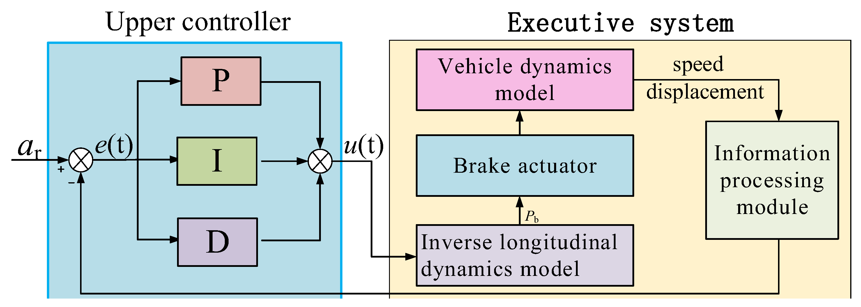
4. Active Brake Controller

4.1. Design of the Upper Controller Based on the Sliding Mode Control

A reasonably expected deceleration significantly impacts the driver and passenger’s safety and comfort during braking. The sliding mode control method is a nonlinear control method of the variable structure control system, with less adjustable parameters, a fast response speed, and a strong ability to suppress external disturbances [29,30,31]. It can efficiently solve complex nonlinear problems and is suitable for generating moderate vehicle deceleration under complex working conditions.
The longitudinal trajectory length of vehicle x and the longitudinal velocity of VRUs relative to the vehicle ( Δ V r , km / h ) are taken as inputs to the upper controller in this paper, and the expected deceleration ( a r , m / s 2 ) is considered the output of the upper controller. The input variables for the upper controller are:
ε = x ε = Δ v r
According to the sliding mode control theory [32,33], the sliding surface is designed to make the control system reach a stable state in a limited time. The sliding surface based on trending law in the limited time for the collision avoidance control system is defined as follows [34]:
S ( t ) = ε + λ 1 ε + λ 2 0 t ε d t
where λ 1 and λ 2 are sliding surface coefficients, and both λ 1 and λ 2 are greater than 0. Taking the derivative of Equation (33), we can obtain:
S ( t ) = Δ v r + λ 1 ε + λ 2 ε
Due to the influence of external disturbance and parameter disturbance in the existing system, for the control system to reach a steady state and make the first derivative of the sliding surface convergent, it is necessary to choose the sliding control rate. Therefore, this paper adopts the symbol function sgn(S) to make the first derivative of the sliding surface convergent, namely:
S = η sgn ( S ) , η > 0
The expected output deceleration a r of the upper controller is:
a r = λ 1 ε + λ 2 ε + η sgn ( S )
The stability of the upper controller can be analyzed by defining the Lyapunov function as follows:
V = 1 2 S 2
Taking the derivative of Equation (37), we can obtain:
V = S S = S η sgn ( S ) = S η
Obviously, when η > 0 , V < 0 . The stability criterion of Lyapunov states that the system is stable and can effectively restrain and weaken the buffeting of the system, which has good robustness against external interference.

4.2. Design of the Lower Controller Based on Discrete PID Control

In order to realize the deceleration of the vehicle, the expected deceleration a r from the output of the upper controller is converted to brake pressure by the lower controller through the inverse longitudinal dynamics model of the vehicle [35,36]. The lower controller must provide robustness to the braking system, and the PID control algorithm can efficiently satisfy the lower controller design requirements. The PID control algorithm consists of proportional control, integral control, and differential control, and the desired deceleration of the upper tracking controller of the vehicle is controlled by adjusting the proportional, integral, and differential coefficients [37,38]. The discrete PID control algorithm presented in this paper is used to design the lower controller; the specific control flow can be seen in Figure 4. The output expression of the lower controller is:
u ( t ) = K p [ e ( t ) + K i n = 0 t e ( n ) + K d ( e ( t ) e ( t 1 ) ) ]
e ( t ) = a r a
where K P , K i , and K d are the proportional coefficient, integral coefficient, and differential coefficient, respectively; e ( t ) is the input of the lower controller; a r is the expected deceleration of the upper controller output; and a is the actual deceleration of the vehicle.
The proportional coefficient K P , the integral coefficient K i , and the differential coefficient K d are adjusted to ensure the control accuracy of the lower controller. At present, the PID parameter adjustment is mainly through two methods: method one is a theoretical calculation method. This method is calculated by accurate mathematical models to determine the PID parameter. The second method of project setting relies primarily on engineering experience. According to engineering experience, the parameters are adjusted by using trial and error in the control system through a lot of number of tests. This study is aimed at a complex multi-objective vehicle control system, and the driving condition is complicated. It is difficult to establish an accurate mathematical model to solve the three parameters of PID control, thus the PID parameters are determined through the project setting method. The specific stages are as follows: Firstly, make K i = 0, K d = 0, K P is set a large initial value, and K P is gradually reduced. The value K P is determined when the vehicle’s actual deceleration rapidly follows the upper controller’s expected deceleration output and does not result in a large overshoot. Secondly, after the K P parameter is determined, the system output of the actual deceleration cannot accurately track the expected deceleration, i.e., there is a steady state error. At this time, the K i value needs to be adjusted to eliminate the error. Therefore, we gradually increase the K i value from zero and observe the size of the steady state error and the status of the system shock. When the system is in a steady state and there is no steady state error, the K i value is determined as the final value. Finally, when the K P and K i values are determined, the K d value should be determined. However, in general project control, the differential coefficient is not set because the actual system exists in the feedback signal noise, and differential control can enlarge noise, making the system produce shock. Therefore, we gradually increase the K d value from zero and find that the tracking effect of the increase in K d on the system is not obvious and the adjustment period becomes longer. Therefore, we set the K d value as 0.

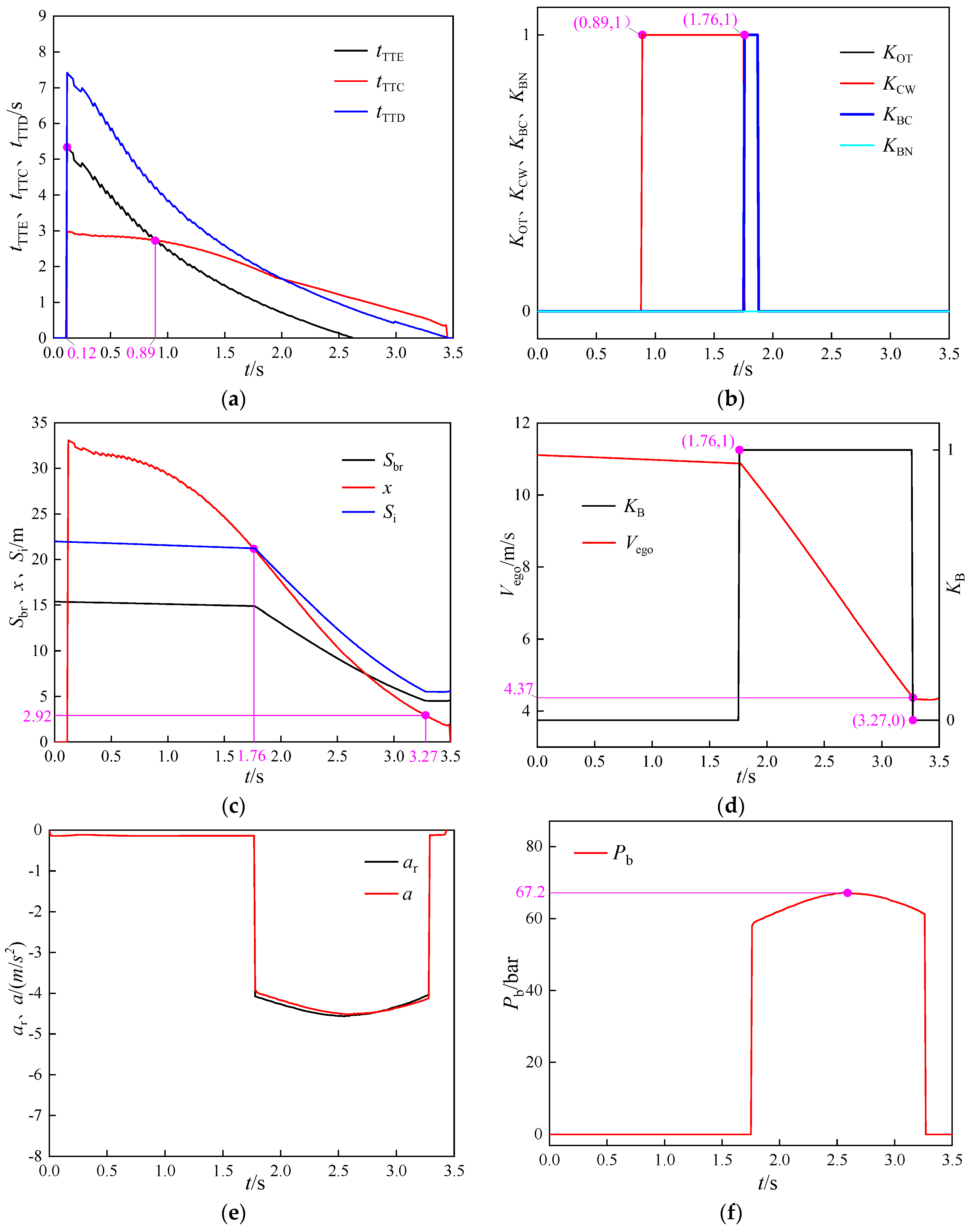
5. Simulation and Verification of the Active Braking Effect under Curved Conditions

Taking electric bicycle riding as the specific research object, the effectiveness of the active collision avoidance system is verified by the joint simulation of Prescan and Matlab/Simulink [39]. The specific simulation process is as follows:
Collision scenarios with curves were set up in the Prescan software. A Honda motorcycle was similar in appearance to the electric bike, therefore, in the Prescan software, the Honda motorcycle was chosen as the electric bicycle simulation vehicle and the Audi A8 was chosen as the automobile simulation vehicle. The Honda motorcycle was set to traverse the road in three motion states: uniform acceleration, uniform deceleration, and uniform speed from the outside or the inside of the curve, and the Audi A8 drove at a speed of 40 km/h on the curve. The millimeter-wave radar sensor was selected to obtain the movement information of the Honda motorcycle, and the millimeter-wave radar sensor was installed at the level of the Audi A8′s front bumper. The specific collision test scenario parameters are shown in Table 1, and the particular parameters of the simulation vehicles are shown in Table 2.
The active collision avoidance control strategy was built in the Matlab/Simulink software. According to the above, in the perception module, when VRUs moved from the outside to the inside or the inside to the outside under the curve conditions, the spatial positions of VRUs relative to the vehicle were built to accurately identify the relative position between them. In the decision-making module, firstly, based on their relative spatial positions, the entry time, departure time, and collision time were calculated for when VRUs move from the outside to the inside or from the inside to the outside under the curve conditions, to compare the three-time relationship and determine whether VRUs are dangerous targets for establishing the safety assessment model. Secondly, the safety distance model, based on the minimum active braking safety distance, the vehicle warning safety distance, and the vehicle active braking safety distance, was constructed to establish the vehicle collision warning signal, the vehicle braking distance sufficient signal, the vehicle braking distance insufficient signal, and the vehicle braking signal, to build the active braking collision avoidance strategy. The upper layer was based on the sliding mode control and the lower layer was based on discrete PID control. The controller parameters were adjusted to make the vehicle output an appropriate deceleration to respond to the corresponding control signal. Finally, the inverse longitudinal dynamic model was built in the execution module. The deceleration input from the execution module was converted to the desired brake pressure, and the desired brake pressure was input through the Prescan interface to control the vehicle deceleration to avoid a collision between the vehicle and the VRUs. The Simulink model is illustrated in Figure 5, and the specific parameters of the collision avoidance strategy are presented in Table 3.
The simulation results of scenario 1 are shown in Figure 6. It can be seen from Figure 6a that when the simulation time t is 0.12 s, the electric bicycle rider is detected by the millimeter-wave radar sensor. When t is 0.89 s, t TTC is between t TTE , t TTD , and K O T = 1 , and the electric bicycle rider is judged to be in a dangerous state. It can be seen from Figure 6b that when t is 0.89 s, K C W = 1 , the active braking system would warn the driver and remind the driver to take braking actions. If the driver still does not take braking actions, it can be seen from Figure 6b,c that when t is 1.76 s, x is between S br and S i , and at this time, K B C = 1 , and the active braking system is activated on the vehicle to start the active braking operation ( K B = 1 ). It can be seen from Figure 6c,d that when t is 3.27 s, the electric bicycle rider rolls out of the vehicle’s driving area and the active braking system stops the active braking operation ( K B = 0 ). At this time, the speed of the vehicle V ego is 4.37 m/s, and the distance from the vehicle to the intersection point M 1 of the electric bicycle track is 2.92 m (The distance from the vehicle to the electric bicycle is x minus half of the width of the electric bicycle, that is: 2.92 − 0.82/2 = 2.51 m), which is greater than the minimum distance d min ( d min = 1 m), that should be maintained between the vehicle and the electric bicycle. Therefore, the vehicle can avoid collision with the electric bicycle. The actual deceleration of the vehicle can follow the expected output of the deceleration by the upper controller, as illustrated in Figure 6e. It can be seen from Figure 6f that the maximum value of the brake pressure P b is 67.2 bar, which is lower than the maximum brake pressure of 150 bar that the brake can output, thus meeting the actual requirements. In scenario 1, the collision avoidance effect of the active braking system is shown in Figure 7.
In scenarios 2 to 6, the changes in V ego , K B , S br , x, and S i are shown in Figure 8. It can be seen from Figure 8b,d,f,h,j that the active braking system stops braking when the simulation time t is 3.32 s, 5.09 s, 4.94 s, 3.65 s, and 3.72 s, respectively. In scenarios 2 to 6, it can be seen from Figure 8a,c,e,g,i that when the simulation time t is 3.32 s, 5.09 s, 4.94 s, 3.65 s, and 3.72 s, respectively, the distance from the vehicle to the intersection point of the electric bicycle track is 2.38 m, 1.76 m, 1.55 m, 2.10 m, and 2.76 m, respectively, and the distance between the vehicle and the electric bicycle is 1.97 m, 1.35 m, 1.14 m, 1.69 m, and 2.35 m, respectively, which is greater than the minimum distance d min ( d min = 1 m) that should be maintained between the vehicle and the electric bicycle. In conclusion, in scenarios 2 to 6, the vehicle could avoid collision with the electric bicycle.
It can be seen from Figure 8b,d,f,h,j that after the active braking system is completed, the vehicle speed V ego is reduced to 6.51 m/s, 2.28 m/s, 2.62 m/s, 5.78 m/s, and 4.59 m/s, respectively, indicating that in all six scenarios, the active braking control strategy proposed in this paper could output reasonable braking deceleration to avoid collision between the vehicle and the electric bicycle.
In scenarios 1 to 6, the actual vehicle deceleration of the lower controller output can quickly track the expected deceleration a r of the upper controller output, as shown in Figure 9, the specific parameters of the upper controller are shown in Table 4, and the specific parameters of the lower controller are shown in Table 5. As shown in Figure 9, the peak braking deceleration of the vehicle in six scenarios is between 2.81 to 4.52 m/s2, which belongs to the medium-low braking intensity [40], and can satisfy passenger comfort.
We conclude that from scenario 1 to scenario 6 when the vehicle is complete, the distance from the vehicle to the VRU is larger than the minimum safe distance, which proves that the proposed active braking collision avoidance strategy can avoid the collision between the vehicle and VRU. Therefore, this study can be effectively applied to the active collision avoidance system for VRUs traversing the road in three motion states of uniform acceleration, uniform deceleration, and uniform speed in curved road conditions, providing a reference for the research on active collision avoidance of vehicles in curved conditions. However, this study does not focus on multiple targets, so it is not appropriate for the study of active vehicle collision avoidance when multiple VRUs traverse the road. To realize this research, it is necessary to construct corresponding models of intelligent vehicle perception modules, the decision-making module, the execution module, and debugging controller parameters to adapt the vehicle's active collision avoidance system under different working conditions.

6. Conclusions

Current active braking system research is primarily focused on protecting the safety of vulnerable road users who traverse the road at a constant speed under straight road conditions. Therefore, this paper has researched active safety collision avoidance for vulnerable road users in uniform acceleration, uniform deceleration, and uniform velocity in curved conditions. Firstly, aiming at curved road conditions, the spatial position relationships between vulnerable road users and the turning vehicle are established when vulnerable road users traverse the road in three motion states of uniform acceleration, uniform deceleration, and uniform speed from the outside of the curve or inside of the curve. Secondly, the mathematical model of time t TTE , time t TTC , and time t TTD of the vulnerable road user are constructed to carry out safety assessments. In order to establish the collision avoidance strategy of the active braking system, the safety distance model of the vehicle is established. Finally, the active braking controller is designed based on sliding mode control of the upper layer and discrete PID control of the lower layer to satisfy the driver’s comfort in the vehicle.
Six kinds of collision test scenarios with curves were constructed to verify the effectiveness of the active braking control system. The simulation results show that when the active braking is completed, the distance from the vehicle to the vulnerable road user is larger than the minimum safe distance ( d min = 1 m), which indicates that the proposed active braking system can effectively avoid collision between the vehicle and vulnerable road users in various motion states. During braking, the peak value of the braking deceleration is between 2.81 and 4.52 m/s2, which belongs to the medium braking intensity, indicating that the designed active braking controller can produce a reasonable braking deceleration and respond to driver comfort. Therefore, based on the results above, this study improves the safety of vulnerable road users when they are traversing the road in various movement states in curved road conditions, and it establishes the baseline conditions and research objectives for the study. Furthermore, this study provides a theoretical foundation and an engineering reference for the research and development of the active braking device for automobiles facing curved road conditions.
Since this study targets a single vulnerable road user in a single movement state, it does not involve the combination of multiple objectives and multiple movement states. Therefore, in future work, to effectively avoid collision between vehicles and multiple moving targets, it is necessary to integrate multiple target motion states to more accurately design the vehicle's active collision avoidance system. Furthermore, in practical applications, when the active collision avoidance system cannot avoid the collision, there is a need to consider how the active collision avoidance system can effectively protect the individuals in the vehicle after the collision and significantly reduce the degree of collision.

Author Contributions

Conceptualization, L.H. and R.G.; methodology, L.H.; software, L.L.; validation, L.L.; formal analysis, L.L.; investigation, L.H.; resources, L.H.; data curation, L.L.; writing—original draft preparation, L.L.; writing—review and editing, L.H. and R.G.; visualization, R.G.; supervision, R.G.; project administration, L.H.; funding acquisition, L.H. All authors have read and agreed to the published version of the manuscript.

Funding

This study was sponsored by the National Natural Science Foundation of China (Grant No. 51805224), the Project funded by China Postdoctoral Science Foundation (Grant No. 2020M671307), the Jiangsu Planned Projects for Postdoctoral Research Funds (Grant No. 2019K043), and the Jiangsu University Advanced Talents Initial Funding Project (Grant No. 15JDG167).

Informed Consent Statement

Informed consent was obtained from all subjects involved in the study.

Conflicts of Interest

The authors declare no conflict of interest.

References

  1. Chen, Q.; Chen, Y.; Bostrom, O.; Ma, Y.; Liu, E. A Comparison Study of Car-To-Pedestrian and Car-To-E-Bike Accidents: Data Source: The China In-Depth Accident Study (CIDAS); Technical Paper: 2014-01-0519; SAE: Hong Kong, China, 2014. [Google Scholar]
  2. Li, Y.W.; Zhang, X.; Wang, W.J.; Ju, X.F. Factors affecting electric bicycle rider injury in accident based on random forest model. J. Transp. Syst. Eng. Inf. Technol. 2021, 21, 196–200. [Google Scholar]
  3. Zhu, X.Y.; Chu, Z.M.; Zhu, D.A.; Zhu, J.A.; Dai, S. China electric bicycle traffic accident analysis and countermeasures. Urban Transp. China 2021, 1906, 64–70. [Google Scholar]
  4. Naci, H.; Chisholm, D.; Baker, T.D. Distribution of road traffic deaths by road user group: A global comparison. Inj. Prev. 2009, 15, 5559. [Google Scholar] [CrossRef] [PubMed]
  5. Guo, F.; Klauer, S.G.; Fang, Y.; Hankey, J.M.; Antin, J.F.; Perez, M.A.; Lee, S.E.; Dingus, T.A. The effects of age on crash risk associated with driver distraction. Int. J. Epidemiol. 2017, 46, 258–265. [Google Scholar] [CrossRef] [PubMed] [Green Version]
  6. Rosén, E.; Sander, U. Pedestrian fatality risk as a function of car impact speed. Accid. Anal. Prev. 2009, 41, 536–542. [Google Scholar] [CrossRef]
  7. Zhao, Y.; Ito, D.; Mizuno, K. AEB effectiveness evaluation based on car-to-cyclist accident reconstructions using video of drive recorder. Traffic Inj. Prev. 2019, 20, 100–106. [Google Scholar] [CrossRef]
  8. Edwards, M.; Nathanson, A.; Wisch, M. Estimate of potential benefit for Europe of fitting Autonomous Emergency Braking (AEB) systems for pedestrian protection to passenger cars. Traffic Inj. Prev. 2014, 15 (Suppl. S1), S173–S182. [Google Scholar] [CrossRef]
  9. Themann, P.; Kotte, J.; Raudszus, D.; Eckstein, L. Impact of positioning uncertainty of vulnerable road users on risk minimization in collision avoidance systems. In Proceedings of the IEEE Intelligent Vehicles Symposium (IV), Seoul, Republic of Korea, 28 June–1 July 2015; pp. 1201–1206. [Google Scholar]
  10. Bachmann, M.; Morold, M.; David, K. On the required movement recognition accuracy in cooperative VRU collision avoidance systems. IEEE Trans. Intell. Transp. Syst. 2020, 223, 1708–1717. [Google Scholar] [CrossRef]
  11. Nkenyereye, L.; Liu, C.H.; Song, J. Towards secure and privacy preserving collision avoidance system in 5G fog-based Internet of Vehicles. Future Gener. Comp. Syst. 2019, 95, 488–499. [Google Scholar] [CrossRef]
  12. Eilbrecht, J.; Bieshaar, M.; Zernetsch, S.; Doll, K.; Sick, B.; Stursberg, O. Model-Predictive Planning for Autonomous Vehicles Anticipating Intentions of Vulnerable Road Users by Artificial Neural Networks. In Proceedings of the IEEE SSCI, Honolulu, HI, USA, 27 November–1 December 2017; p. 18. [Google Scholar]
  13. Park, M.K.; Lee, S.Y.; Kwon, C.K.; Kim, S.W. Design of Pedestrian Target Selection with Funnel Map for Pedestrian AEB System. IEEE Trans. Veh. Technol. 2017, 665, 3597–3609. [Google Scholar] [CrossRef]
  14. Guo, L.; Ren, Z.J.; Ge, P.S.; Chang, J. Advanced emergency braking controller design for pedestrian protection oriented automotive collision avoidance system. Sci. World J. 2014, 2014, 218–246. [Google Scholar]
  15. Li, J.X.; Yao, L.; Xu, X.; Cheng, B.; Ren, J.K. Deep reinforcement learning for pedestrian collision avoidance and human-machine cooperative driving. Inform. Sci. 2020, 532, 110–124. [Google Scholar] [CrossRef]
  16. Lee, H.K.; Shin, S.G.; Kwon, D.S. Design of emergency braking algorithm for pedestrian protection based on Multi-Sensor Fusion. Int. J. Automot. Technol. 2017, 186, 1067–1076. [Google Scholar] [CrossRef]
  17. Zadeh, R.B.; Ghatee, M.; Eftekhari, H.R. Three-Phases Smartphone-Based Warning System to Protect Vulnerable Road Users Under Fuzzy Conditions. IEEE Trans. Intell. Transp. Syst. 2017, 19, 2086–2098. [Google Scholar] [CrossRef]
  18. Duan, J.L.; Li, R.J.; Hou, L.; Wang, W.J.; Li, G.F.; Li, S.E.; Cheng, B.; Gao, H.B. Driver braking behavior analysis to improve autonomous emergency braking systems in typical Chinese vehicle-bicycle conflicts. Accid. Anal. Prev. 2017, 108, 7482. [Google Scholar] [CrossRef] [PubMed]
  19. Peng, Y.; Yu, W.F.; Wang, X.H.; Xu, Q.; Wang, H.G.; Wu, W.G. AEB effectiveness research methods based on reconstruction results of truth Vehicle-to-TW accidents in China. Proc. Inst. Mech. Eng. Part D J. Automob. Eng. 2021, 235, 2029–2039. [Google Scholar] [CrossRef]
  20. Pan, C.H. Research on Pedestrian-Vehicle Interaction Strategies of Autonomous Vehicles. Master’s Thesis, Zhejiang University, Zhejiang, China, 2021. [Google Scholar]
  21. Wang, J.J.; Guo, W.B.; Zhang, Y.S. Simulation and verification of the control strategies for Pedestrian Active Collision Avoidance system based on V2X. Automob. Technol. 2022, 5, 4149. [Google Scholar]
  22. Li, M.H. Research on Pedestrian Collision Avoidance Method for Intelligent Vehicle Based on V2X in Occlusion Environment; Beijing Institute of Technology: Beijing, China, 2018. [Google Scholar]
  23. Yuan, C.C.; Song, J.H.; He, Y.G.; Jie, S.; Chen, L. Active collision avoidance algorithm of autonomous vehicle based on pedestrian trajectory prediction. J. Jiangsu Univ. 2021, 42, 1–8. [Google Scholar]
  24. Hallmark, S.; Goswamy, A.; Litteral, T.; Hawkins, N.; Smadi, O. Evaluation of sequential dynamic chevron warning systems on rural Two-Lane curves. Transport. Res. Rec. 2020, 2674, 648–657. [Google Scholar] [CrossRef]
  25. Wang, B.; Hallmark, S.; Savolainen, P. Crashes and Near-Crashes on horizontal curves along rural Two-Lane highways: Analysis of naturalistic driving data. J. Saf. Res. 2017, 6312, 163–169. [Google Scholar] [CrossRef]
  26. Qu, C.; Qi, W.Y.; Wu, P. A High Precision and Efficient Time-to-Collision Algorithm for Collision Warning Based V2X Applications. In Proceedings of the 2018 and International Conference on Robotics and Automation Sciences (ICRAS 2018), Wuhan, China, 23–25 June 2018. [Google Scholar]
  27. Lopez, A.; Sherony, R.; Chien, S.; Li, L.X.; Yi, Q.; Chen, Y.B. Analysis of the Braking Behavior in Pedestrian Automatic Emergency Braking. In Proceedings of the IEEE International Conference on Intelligent Transportation Systems, Gran Canaria, Spain, 15–18 September 2015. [Google Scholar]
  28. Zhang, X.; Yang, W.; Tang, X.; Wang, Y. Lateral distance detection model based on convolutional neural network. IET Intell. Transp. Syst. 2018, 13, 3139. [Google Scholar] [CrossRef]
  29. Mobayen, S.Y. Fast terminal sliding mode controller design for nonlinear second-order systems with time-varying uncertainties. Complexity 2015, 21, 239–244. [Google Scholar] [CrossRef]
  30. Ebrahimi, N.; Ozgoli, S.; Ramezani, A. Model-free sliding mode control, theory and application. Proc. Inst. Mech. Eng. Part I J. Syst. Control. Eng. 2018, 232, 1292–1301. [Google Scholar] [CrossRef]
  31. Liang, B.; Zhu, Y.Q.; Li, Y.R.; He, P.J.; Li, W.L. Adaptive nonsingular fast terminal sliding mode control for braking systems with Electro-Mechanical actuators based on radial basis function. Energies 2017, 10, 1637. [Google Scholar] [CrossRef] [Green Version]
  32. Bandyopadhyay, B.; Janardhanan, S. Discrete-Time Sliding Mode Control: A Multidate Output Feedback Approach. In Lecture Notes in Control and Information Sciences; Springer: Berlin/Heidelberg, Germany, 2005. [Google Scholar]
  33. Shtessel, Y.; Fridman, L.; Plestan, F. Adaptive sliding mode control and observation. Int. J. Control. 2016, 89, 1743–1746. [Google Scholar] [CrossRef]
  34. Liu, X.; Sun, X.X.; Dong, W.; Yang, P.S. A new discrete-time sliding mode control method based on restricted variable trending law. Acta Autom. Sin. 2013, 39, 1552–1557. [Google Scholar] [CrossRef]
  35. Baek, W.; Song, B. Design and validation of a longitudinal velocity and distance controller via hardware-in-the-loop simulation. Int. J. Automot. Technol. 2009, 10, 95–102. [Google Scholar] [CrossRef] [Green Version]
  36. Lee, M.H.; Park, H.G.; Lee, S.H.; Yoon, K.S.; Lee, K.S. An adaptive cruise control system for autonomous vehicles. Int. J. Precis Eng. Man. 2013, 14, 373–380. [Google Scholar] [CrossRef]
  37. Gounis, K.; Bassiliades, N. Intelligent momentary assisted control for autonomous emergency braking. Simul. Model. Pract. Theory 2021, 115, 102–450. [Google Scholar] [CrossRef]
  38. Yang, W.; Zhang, X.; Lei, Q.; Cheng, X. Research on longitudinal active collision avoidance of autonomous emergency braking pedestrian system (AEB-P). Sensors 2019, 19, 4671. [Google Scholar] [CrossRef]
  39. Zhang, M.F.; Li, M.; Chen, Z.F.; Wang, P.W.; Cheng, W.D. Left-turn motion planning of autonomous vehicles at unsignalized intersections in an environment of heterogeneous traffic flow containing autonomous and Human-driven vehicles. China J. Highw. Transp. 2021, 347, 6778. [Google Scholar]
  40. Yang, W.; Zhao, H.Y.; Shu, H. Simulation and verification of the control strategies for AEB pedestrian collision avoidance system. J. Chongqing Univ. 2019, 422, 1–10. [Google Scholar]
Figure 1. Schematic diagram of the movement of the vehicle and VRU: (a) a VRU crosses the road from the outside to the inside of the curve; (b) a VRU crosses the road from the inside to the outside of the curve.
Machines 11 00100 g001
Figure 2. The curve of brake pedal force F P , braking deceleration a, and braking time t.
Machines 11 00100 g002
Figure 3. Automobile collision avoidance strategy.
Machines 11 00100 g003
Figure 4. Control flow graph of the upper-layer controller.
Machines 11 00100 g004
Figure 5. Matlab/Simulink Simulation model.
Machines 11 00100 g005
Figure 6. The simulation results of scenario 1. (a) The changes in t T T C , t TTE , and t TTD . (b) The changes in K O T , K C W , K B C , and K B N . (c) The changes in S b r , x, and S i . (d) The changes in V ego and K B . (e) The changes in a r and a . (f) The change in P b .
Machines 11 00100 g006
Figure 7. (a) Without an active braking system; (b) With an active braking system.
Machines 11 00100 g007
Figure 8. Simulation results of scenarios 2 to 6. (a) The changes in S br , x , and S i in scenario 2. (b) The changes in V ego and K B in scenario 2. (c) The changes in S b r , x , and S i in scenario 3. (d) The changes in V ego and K B in scenario 3. (e) The changes in S b r , x , and S i in scenario 4. (f) The changes in V ego and K B in scenario 4. (g) The changes in S b r , x , and S i in scenario 5. (h) The changes in V ego and K B in scenario 5. (i) The changes in S b r , x , and S i in scenario 6. (j) The changes in S br , x , and S i in scenario 6.
Machines 11 00100 g008aMachines 11 00100 g008b
Figure 9. The changes in ar and a in: (a) scenario 1, (b) scenario 2, (c) scenario 3, (d) scenario 4, (e) scenario 5, and (f) scenario 6.
Machines 11 00100 g009
Table 1. Specific Parameters of Crash Test Scenarios.
Collision ScenariosVehicle Speed
(km/h)
Electric Bicycle Initial Velocity (km/h)Electric Bicycle Motion StatusElectric Bicycle Acceleration (m/s)Electric Bicycle Sports Direction
Scenarios 14020Uniform acceleration1.2From the outside to the inside of the curve
Scenarios 24020Uniform acceleration1.2From the inside to the outside of the curve
Scenarios 34030Uniform deceleration−1.2From the outside to the inside of the curve
Scenarios 44030Uniform deceleration−1.2From the inside to the outside of the curve
Scenarios 54025Uniform speed0From the outside to the inside of the curve
Scenarios 64025Uniform speed0From the inside to the outside of the curve
Table 2. Specific vehicle and electric bicycle parameters.
Simulation VehicleWheelbase/mDistance from Centroid to front Axle/mDistance from Centroid to Rear Axis/mCentroid Height/mQuality/kgLength/mWidth/mMaximum Braking Pressure/bar
vehicle2.941.171.770.5518205.22.0150
electric bicycle1.50.8210.6790.5952972.20.8280
Table 3. Specific collision avoidance strategy parameters.
Collision Avoidance Strategy Parameters
t g / s t g / s t dr / s d min / M
0.20.021.61.0
Table 4. Specific upper controller parameters.
Symbol λ 1 λ 2 η
Value0.70.30.01
Table 5. Specific lower controller parameters.
Collision Scenarios K P K i K d
Scenario 112.50.40
Scenario 212.50.40
Scenario 3120.40
Scenario 4120.40
Scenario 512.50.30
Scenario 612.50.30
Disclaimer/Publisher’s Note: The statements, opinions and data contained in all publications are solely those of the individual author(s) and contributor(s) and not of MDPI and/or the editor(s). MDPI and/or the editor(s) disclaim responsibility for any injury to people or property resulting from any ideas, methods, instructions or products referred to in the content.

