Article

Federated Multi-Model Transfer Learning-Based Fault Diagnosis with Peer-to-Peer Network for Wind Turbine Cluster

School of Mechanical Engineering and Automation, Harbin Institute of Technology (Shenzhen), Shenzhen 518000, China
*
Author to whom correspondence should be addressed.
Machines 2022, 10(11), 972; https://doi.org/10.3390/machines10110972
Submission received: 16 September 2022 / Revised: 20 October 2022 / Accepted: 21 October 2022 / Published: 24 October 2022
(This article belongs to the Special Issue Machine Learning for Fault Diagnosis of Wind Turbines)

Abstract

:
Intelligent fault diagnosis for a single wind turbine is hindered by the lack of sufficient useful data, while multi-turbines have various faults, resulting in complex distributions. Collaborative intelligence can better solve these problems. Therefore, a peer-to-peer network is constructed with one node corresponding to one wind turbine in a cluster. Each node is equivalent and functional replicable with a new federated transfer learning method, including model transfer based on multi-task learning and model fusion based on dynamic adaptive weight adjustment. Models with convolutional neural networks are trained locally and transmitted among the nodes. A solution for the processes of data management, information transmission, model transfer and fusion is provided. Experiments are conducted on a fault signal testing bed and bearing dataset of Case Western Reserve University. The results show the excellent performance of the method for fault diagnosis of a gearbox in a wind turbine cluster.

1. Introduction

Fault diagnosis of rotating machinery plays a vital role in the entire life cycle of machines, which monitors operation processes, analyzes operation data, and provides reasonable maintenance suggestions [1,2,3]. For wind turbines, due to the particularity of the working scene, the uncertainty of working conditions, and the high cost of operation and maintenance, it is essential to monitor the different states during operations. Wind turbine farms are located in remote areas that have abundant wind energy resources but poor natural conditions. It is far among the turbines, and it is difficult to monitor each wind turbine in real time. Moreover, the problem of information exchange in the cluster is prominent when turbines are running, and the amount of data generated by wind turbines in actual operation is on a large scale, resulting in significance difficulties in data management, storage, calling, and transmission.
The key point of current research on wind turbine fault diagnosis is that it is difficult to extract and analyze fault knowledge under complex working conditions among various wind turbines in a wind turbine cluster [4,5]. In the actual industry, fault data from a single turbine are limited and cannot contain all fault information of various fault states, forms, and periods. There is still a sparsity problem of more normal data without fault but fewer fault data. When modeling only by a single turbine, obstacles such as low accuracy, weak generalization ability, and weak robustness caused by an insufficient amount of fault data make the model unsuitable for application. In contrast, in a wind turbine cluster, different turbines are in various states. Through local modeling of each turbine in a cluster, transmitting model information, and fusing the model, the fault knowledge of each wind turbine is stored with collaborative intelligence [6,7] so that it can be better applied to operation state monitoring and the operation data analysis of each turbine. Collaborative intelligence or swarm intelligence are used to solve the problems that hinder the model training and optimizating in the mode of single machine intelligence.
For the fault diagnosis of wind turbine clusters, there are some limitations and obstacles in modeling and fault diagnosis owing to complex structures, working conditions, and other practical factors.
First, for the problem of data sparsity, commonly used methods are mostly from the perspective of sample expansion [8,9]. The research content is mainly the difference between the original samples and the newly generated samples and how to reduce this difference. However, such a difference varies in different states of turbines in a cluster and is difficult to determine, which hinders the modeling and training process.
Second, for complex working conditions in clusters, existing solutions mainly focus on transfer learning (TL) [10,11]. The concept of the domain in transfer learning corresponds to the different working conditions in the fault diagnosis problem. It typically uses the knowledge learned in one data domain by the fault diagnosis model to solve the problem in another data domain. Commonly applied transfer learning is mostly used for the data processing and mining of a single wind turbine, but it involves fewer wind turbine individuals.
Third, for the model fusion process, most existing methods focus on more traditional ensemble learning (EL) [12,13] and federated learning (FL) [14,15]. Voting, in which the minority obeys the majority, is the most widely used in EL. FL is a distributed model-training instance that sets up multiple federated participants and has a central server for model fusion. Such methods are usually set under ideal conditions and seldom consider external interference in the actual process of model training. The performance of the model corresponding to the average weight did not reach its best state.
To solve such problems, a peer-to-peer network (P2PNet) [16] is constructed for the wind turbine cluster, where each node corresponds to a wind turbine. A P2PNet is a computer network that assigns tasks, data, and work among peers in the entire network. The network consists of peers and the information transmission channels among peers. Each participant is equal and has the ability to communicate with other peers.
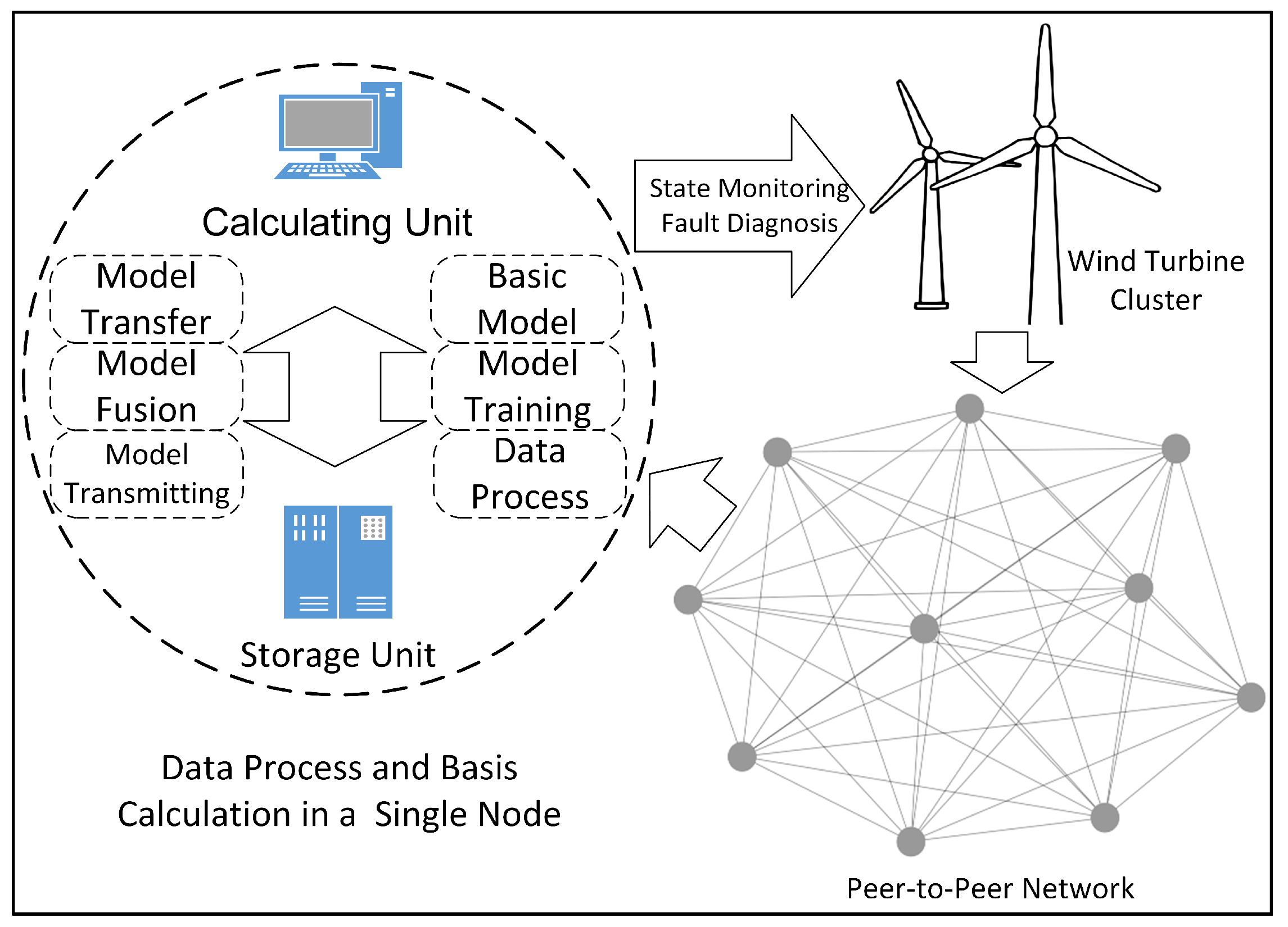
In the P2PNet, a fault diagnosis framework for a wind turbine cluster is proposed as shown in Figure 1, where raw data are saved locally in distributed storage. A calculating unit for computing and storage unit for data storage are configured in each node. Each node is equivalent and has functional replicability, including data preprocessing, model configuration, training, transferring, fusion, and transmission. In addition, multi-task learning (MTL) is introduced, and a dynamic adaptive outlier monitoring process and weight adjustment method is proposed in this process. The final results of fault diagnosis models are to configured for state monitoring and fault diagnosis of the wind turbine cluster.
The core contributions and highlights of this paper can be listed as follows.
(1)
In a situation of insufficient labeled samples and complex working conditions, a fault diagnosis framework and method with a peer-to-peer network for a wind turbine cluster has been proposed based on multiple model transfer and dynamic adaptive weight adjustment fusion (MMT-DAWA).
(2)
Considering the different data distributions between wind turbines in a cluster resulting from various working conditions and environments, multi-task transfer-based elastic weighted consolidation with a fisher information matrix constricting model parameters has been introduced to reduce the impact of domain drift.
(3)
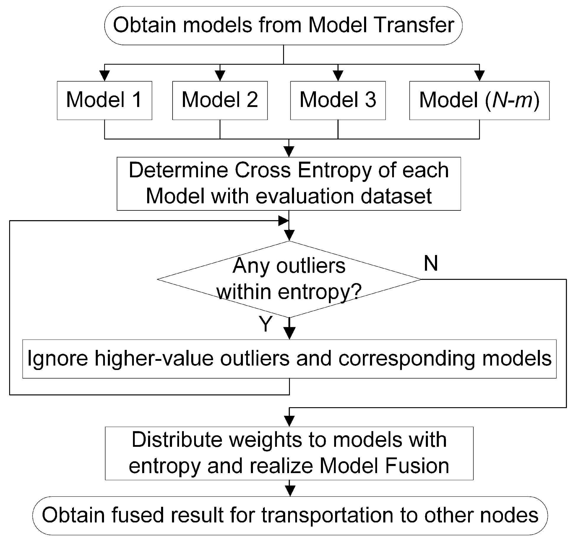
To decrease the influence of noise on the model training process at each turbine in a cluster, a modified dynamic adaptive weight adjustment model fusion method based on a federated average algorithm has been proposed, with model processes of outlier monitoring, determination of evaluation criteria for outliers, and weight distribution.
The remainder of this paper is organized as follows. Section 2 presents related works with some research and applications related to the topic. Section 3 describes the proposed algorithm and model training process. Section 4 presents the experiment, discussing the model performance and analysis of the proposed method. Section 5 concludes the study and proposes the future research directions.

2. Related Works

Artificial intelligence has greatly improved the model performance and diagnostic accuracy in condition monitoring and fault diagnosis [17]. A great number of studies on intelligent fault diagnosis adapting to a single machine [18,19] instead of multiple machines in a cluster have been carried out. Several methods of traditional machine learning (ML) have been applied [20,21,22] to solve the problems of fault diagnosis such as the hidden Markov model, support vector machine, gray neural network, and artificial neural network. With the development of ML and the computing ability of modern computers in the big data era, the idea of deep learning (DL) [23] has been applied. Common DL networks include convolutional neural networks [24], recurrent neural networks [25], sparse auto encoders [26], and generative adversarial networks [27]. When considering the situation of non-independent and identically distributed (Non-IID) data under various working conditions, TL with knowledge transfer is introduced to the process of fault diagnosis [28].
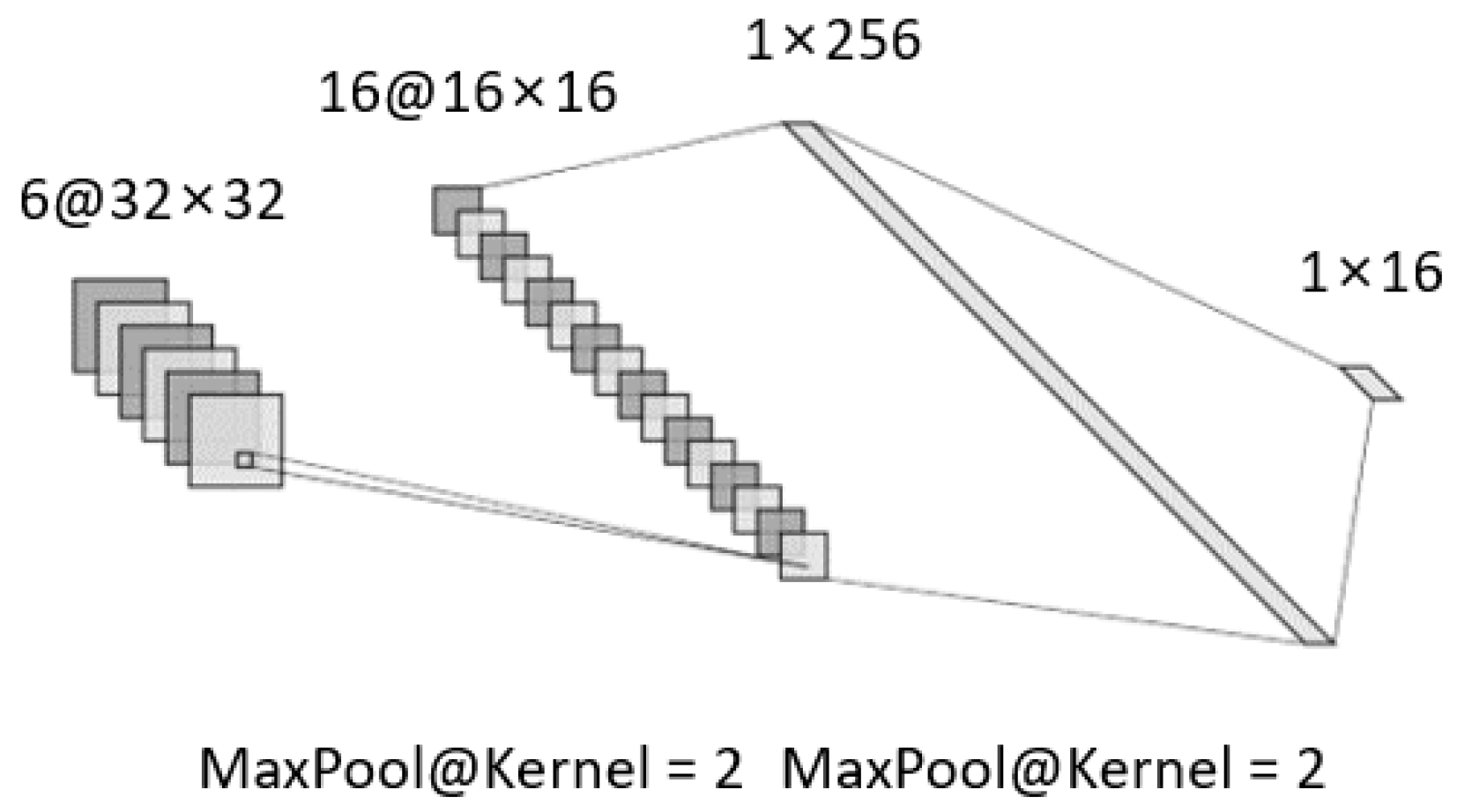
Among them, convolutional neural network (CNN) [29] is broadly used in the pattern recognization and fault diagnosis, which contains a convolution layer, a pooling layer, and a fully connected layer. Combined with the convolution calculation, the number of model parameters is reduced compared with that of the fully connected layer. In the network training process, the cross-entropy loss is often selected for backpropagation. During model training, the updating form of the model parameters often adopts the stochastic gradient descent (SGD) algorithm with momentum, which introduces a momentum accumulating historical gradient information based on traditional SGD to speed up the processing of gradient descent. It accumulates the average moving value of the current gradient and all previous gradient exponential attenuation and continues to move in this direction.
Traditional methods rely on single machines and simple conditions of a wind turbine, whereas fusion methods are required in multi-machines corresponding to various conditions of wind turbine clusters. A reasonable and effective approach to information exchange is essential for a wind turbine cluster. There are two mainstream methods of information exchange within clusters: data exchange and model exchange.
Data exchange indicates gathering all the local data of different machines as one dataset, modeling uniformly, and updating the parameters with model training. In such cases, TL is broadly used with excellent performance when there are different feature spaces or distributions between the source and target data [30]. A popular explanation of TL is to transfer the knowledge learned through the training model in one data domain to another data domain to solve the corresponding problems. In TL, different domains are defined according to different feature spaces or edge probability distributions. In mechanical fault diagnosis, the data fields corresponding to different machine operating conditions, locations, and machine individuals can be regarded as different domains. Different tasks have different label spaces, corresponding to different fault types, states, and degrees. A large number of TL applications for fault diagnosis have been carried out, and excellent results have been obtained from model training and experiments [31,32,33]. In addition to transfer fault diagnosis methods focusing on the adaptation of a single source domain, in an actual industrial scene, multiple labeled source domains can be obtained in a wind turbine cluster. Therefore, researchers have proposed methods of multi-source domain transfer learning fault diagnosis [34], adversarial domain adaptation with classifier alignment [35], and so on. Such a mode of data exchange makes the evaluation criteria more standardized and unified, and model training for fault diagnosis is more convenient to manage. However, considering multiple wind turbines in a cluster, the raw data of each turbine proportionally increase the amount of data, resulting in a high cost of data storage, low data transmission efficiency, and low quality and efficiency in data management.
Model exchange refers to fusing the models in different machines into a more comprehensive model through the relevant algorithms of model fusion, saving raw operation data locally and conducting model training at each turbine. Ensemble learning is an effective way to deal with voting, bagging and boosting. In addition, to improve the classification accuracy when the training data are insufficient, researchers have proposed an ensemble transfer learning (ETL) framework [36], which combines the methods of TL and EL. A large number of applications of EL or ETL for machine fault diagnosis have been reported in recent years [37,38,39,40]. However, owing to data distribution differences, data volume differences, and fault data sample differences, there are still obstacles to the applications of fault diagnosis in wind turbine clusters such as efficiency in data management and calling, and the accuracy of the fused model of the ensemble. With technological progress in the era of big data, federated learning [41], industrial Internet of Things [42,43], and cloud-edge collaborative computing [44] have been applied to fault diagnosis research. FL is a branch of ML with the purpose of decentralization [45], which focuses on building and optimizing diagnosis models in the situation of distributed datasets, constructing the corresponding federated network, and using the distributed data of each node in the network to improve the overall model performance.
Ideally, the intelligent fault diagnosis method for large-scale wind turbine clusters does not consider data communication problems, such as channel width and data flow. However, in industrial and practical applications, owing to the hardware structure and other factors, information transmission in fault diagnosis networks is limited. Therefore, researchers have proposed effective FL frameworks and algorithms to solve the problem of obstacles [46,47,48]. These methods rely on simple working conditions and operating environments, and it is impossible to obtain excellent results in complex situations. In a wind turbine cluster, various turbines possess various distributions of data, so TL has been introduced to the methods in the cluster combined with FL frameworks, called federated transfer learning (FTL), where models perform excellently in fault diagnosis in clusters [49,50,51].
However, the lack of constraining model parameters leads to an uncertain convergence rate, low recognition accuracy of the model, and weak generalization ability. Therefore, to accurately locate, identify, classify, and predict the fault development trend in the entire life cycle of a wind turbine gearbox, it is essential to deal with the balance between the management, calling of a huge dataset, and application of big data for gearbox fault diagnosis under complex working conditions in a wind turbine cluster.

3. Methodology

Each node in the P2PNet is equal, so the function at one node needs to be studied and then extended to the entire network. The process in one node can be divided into three sub-modules: information transmission structure, model transfer with fault knowledge, and model fusion with dynamic adjustment method.

3.1. Basic Structure and Model

In P2PNet, a method of multiple model transfer and dynamic adaptive weight adjustment (MMT-DAWA) model fusion used in intelligent fault diagnosis in a single node is proposed, which comprises three steps, as shown in Figure 2. When receiving models from other nodes, the current node abandons some of them to reduce the impact of the uncertainty. Then, considering that data among nodes in the actual industry are Non-IID, a model transfer-based MTL process is proposed. After obtaining several models from the transfer step, the current node implements model fusion with a dynamic adaptive model selection and adaptive weight adjustment. Finally, a better result corresponding to a specific task is obtained, and each node implements the model output in iteration.
CNN with a strong ability in pattern recognization and fault diagnosis is selected as the basic diagnostic model. As shown in Figure 3, to reduce the amount of model data while ensuring model performance, a small and shallow CNN [29] is constructed, which is composed of two convolution layers, two max-pooling operations, and two fully connected layers. The numbers of channels of the convolution and fully connected layers are 6, 16, 256, and 16, respectively, and the sizes of the two convolutional cores are all 5 × 5 .
In addition, the leaky-ReLU function [52] is adopted as the activating function with the coefficient of the negative axis of the function being 0.01. The Leaky-ReLU function changes the distribution of the flow data in the neural network, and the Kaiming initialization method [53] is selected to solve this problem.

3.2. Knowledge Transfer between Nodes Based on MTL

3.2.1. Non-IID Tasks

In actual industry, different turbines may contain a few types rather than all types of fault data. The fault degree and depth are different owing to the varying working conditions of different wind turbines. The fault degree and depth describe the fault severity of machine parts from qualitative and quantitative perspectives. The degree could be described as “Heavy”, “Moderate”, and “Light”, while the depth needs to be described with the specific fault diameters and depths. Therefore, data are defined as Non-IID according to various conditions, and the data distribution of each wind turbine is different in a real industrial scene. To reduce this difference, a TL method is used for knowledge mining from raw data with different edge distributions to facilitate the deep fusion of fault knowledge. TL is broadly divided into four categories: instance-based, feature-based, model-based, and relationship-based [54]. The other three consider the transfer of fault knowledge from the perspective of data or features, whereas only the model-based TL method considers model parameters. In this study, for the fault diagnosis task of wind turbine clusters, the problems of sparse samples, variable working conditions, data management, and sharing in real industrial scenarios must be considered. Therefore, a way of model exchange rather than data exchange is determined and model-based deep transfer learning, which is based on the assumption that some labeled instances in the target domain should be available in the target model training process, is considered.
The data domain responsible for model training in the TL is called the source domain, and the transferred object is called the target domain. The distribution difference between the source and target domain is called domain drift. Figure 4 describes the basic concepts of TL within the framework of a cluster. If the trained model, the classifier in the source domain, is directly taken to the target domain, some misclassifications of samples appear owing to the existence of domain drift, which leads to the failure of the algorithm and poor diagnosis performance in the actual working conditions. In a cluster, the data of each node are saved locally, and the information exchanged between nodes involves only the trained models. Multi-task learning (MTL) [55] is selected for the adaptive process of the target domain, which realizes multiple objective tasks and improves the generalization with the domain knowledge contained in the supervised signal of related tasks.

3.2.2. Cross-Node Model Transfer

When a certain node in the network receives several models from other nodes, it randomly selects some of them to reduce the impact of the uncertainty. Assuming that there are N nodes in the cluster network except for the current node, the models of m nodes are removed, so the remaining ( N m ) models are used in the subsequent process.
The adaptive problem in the target domain is regarded as an MTL problem. Among them, task M requires that the overall model of all transfer processes performs well, and the task N with several sub-tasks requires that the model of each sub-task of the transfer process performs well. An adaptive model A optimized for task N is defined, which is initialized with the source domain model from the corresponding node. A source domain model B for the initialization of the transfer process is also defined.
Within the MTL, the elastic weight consolidation (EWC) method is introduced to adjust and constrain the model parameters, and the Fisher information matrix (FIM) is selected as the constraint on the model parameters to adapt to the overlap between different distributions. The FIM is a generalization of the Fisher information from a single parameter to multiple parameters. Fisher information represents the average amount of information about state parameters that can be provided by a sample of random variables in a certain sense. Assuming that the model parameter θ is a vector, which models the distribution p ( x | θ ) , the learning process maximizes the likelihood of p ( x | θ ) and θ . To evaluate the estimation of θ , a score function (SF) is defined as shown in Equation (1).
s ( X ; θ ) = θ log p ( X | θ ) = i = 1 n log f ( X i ; θ ) θ ,
where p is the probability distribution of model assumptions, X is the raw data variable and θ is the vector of model parameters. The SF is the gradient of the log-likelihood function, and the definition of FIM is based on it. FIM is defined as the second-order moment of the SF as shown in Equation (2), where E is the mathematical expectation.
F ( θ ) = E [ s ( X ; θ ) E s ( X ; θ ) ] 2
In the target domain, FIM is used to constrain the model parameters to realize the adaptive process, and the degree of importance between tasks λ is introduced to it. Moreover, loss in source domain models should be considered so that a penalty coefficient β is introduced to constrain the loss values in the source domain. The adaptive loss function of the target domain is shown in Equation (3).
L ( A , x ) = L C E ( A , x ) + λ 2 i F i ( A i B i ) 2 + β L C E ( B , x ) ,
where L C E represents the cross-entropy loss, λ is the degree of importance between task M and task N , β represents the penalty coefficient of source model loss, F represents the Fisher Information Matrix, A is the model to be updated in the target domain, and B is the updated model in the source domain.

3.3. Dynamic Fusion within Multiple Models

3.3.1. Framework of Model Fusion

Considering the presupposition of specific scenes, FL is determined to be the basic framework for model fusion. It can better satisfy the requirements of wind turbine cluster fault diagnosis in terms of data management, information transmission, and model fusion. The core of model fusion is that each model is given a certain weight, multiplied by the corresponding parameters, and finally summed, as shown in Equation (4).
G ( x ) = i = 1 N w i · g i ( x ) ,
where N represents the number of models to be fused, w represents the weight of each client model and g ( x ) represents the parameters of each model. The most frequently used weights distributing mode is average weighting, as shown in Equation (5), where N represents the number of models.
w i = 1 N , i = 1 , 2 , , N
The average weighting mode cannot resist experimental process error but accumulates such errors, propagateing forward and backward. This makes it unable to adapt and deal with changes in the external environment. In addition, before model fusion, each node must be able to judge and analyze the performance and effectiveness of the models obtained from the previous steps. During model fusion, the weights given to different models should also be different, which will help to realize the advantages of better models and avoid the disadvantages of worse models. Therefore, a dynamic adaptive weight adjustment (DAWA) model fusion method is developed as shown in Figure 5.
At each node, after the transfer stage, ( N m ) models are obtained. Then, the cross-entropy of each model output is determined as the evaluation criterion as performance is negatively related to the entropy. Subsequently, each entropy is adapted to determine whether there is a higher-value outlier. If so, then the corresponding model is ignored in the current iteration step. After k higher-value outliers are ignored, the weights corresponding to the remaining ( N m k ) models are distributed according to the relative size of each entropy. Finally, model fusion is conducted for corresponding tasks. Within these processes, two main operations are included. One is dynamic adaptive outlier monitoring and model selection, and the other is adaptive weight adjustment and model fusion.

3.3.2. Dynamic Adaptive Outlier Monitoring and Model Selection

The dynamic adaptive method mainly calculates the cross-entropy of each model output and conducts some process. The entire method is presented in Algorithm 1.
The core calculation content of the algorithm is variance as shown in Equation (6), where E represents the expectation and X represents the data of samples.
v a r X = E [ ( X E ( X ) ) 2 ]
Two variances are calculated: v a r 1 of the current entropy array and v a r 2 of the remaining array after removing the maximum value on the current basis. The comparison between the variance changing ratio and the evaluation threshold is shown in Equation (7).
v a r 1 v a r 2 v a r 1 ? ε ,
where question mark “?” represents the comparison of the two sides, and ε is the evaluation threshold to judge whether a value is an outlier. If the variance change rate (left-hand side of equation) is greater than the evaluation criterion ε (right-hand side of equation), the maximum value in the current array is a higher-value outlier. Accordingly, the corresponding model parameters should be discarded during model fusion.
Algorithm 1 Dynamic adaptive outlier monitoring and model selection.
Machines 10 00972 i001
If ε is extremely large, the variance-changing rate cannot exceed it in all possible cases. So, the algorithm determines that there are no outliers, which may cause the overall model accuracy to be reduced because experimental errors are accumulated. If ε is too small, the rate of change can easily exceed it when the variance changes slightly, so the algorithm determines there are outliers. This may result in ignoring and discarding too many models, leading to information loss. Outliers should be selected to ensure the information reliability, but more information should not be ignored in a large area to avoid information loss. Therefore, it is necessary to determine the appropriate ε . The specific value is determined by big data analysis and polynomial fitting.
As shown in Algorithm 2, ε is determined by random big data which vary from 0 to 1 in steps of 0.001. The testing epoch of each value is 100,000 and different random numbers are generated in every epoch to replace arrays with different entropy values.
The reason for randomly generating arrays instead of true entropies is that data are easy to access. The actual training is complex and time-consuming, which cannot meet the preset requirements of 100,000 test epochs for each ε . Moreover, regardless of the variation range, data complexity, data randomness or relative size, the random number is larger than the true entropy, which ensures the integrity of the information.
The cross-entropies of model output are usually distributed between 0 and 1 and vary in a small range, so random numbers from 0 to 1 are generated. Meanwhile, about 10,000 sets of actual experiments are conducted, and the cross-entropies are recorded for comparison, as shown in Table 1. The generated data meet the experimental requirements, which ensures the information integrity and the authenticity of the generation.
Algorithm 2 Determining of ε in Algorithm 1.
Machines 10 00972 i002
Algorithm 1 is used in several rounds of testing. The k corresponding to each ε and the percentage p i of each k are recorded. In addition, p i is shown in Equation (8).
p i = n i e p o c h · 100 , ( i = 1 , 2 , , k ) ,
where k represents the number of outliers, n i represents the number of epochs corresponding to k, and e p o c h represents the whole testing epoch. When analyzing ε , it is processed based on the column k = 0 , i.e., there are no outliers. To meet the principle of 3 σ , all lines with a percentage greater than 99.73% are removed, and the remaining data index is redistributed. Then, for each ε , the percentage is multiplied by the corresponding k and a coefficient α . Finally, we add them together with the percentage when k = 0 to obtain ε corresponding to the smallest number, as shown in the following Equation (9).
ε i n d e x = a r g m i n ( N + p 0 + i = 1 N p i · i · α ) ,
where N is the number of models, p i is the percentage corresponding to k = i , ( i = 0 , 1 , 2 , , k ) , and α is the ratio coefficient, reducing the proportion of the larger k and the range of the ignored clients. Similar to ε , the big data method is adopted in determining α with a value varying from 0.9 to 1 in steps of 0.001. Combined with Algorithm 2, the best-fitted ε under different N and the average of the percentage when k = 0 are calculated. Finally, the maximum value that satisfies the 3 σ principle is obtained. α is found to be 0.954.
An appropriate ε has a one-to-one correspondence with the number of models in the cluster. Polynomial fitting is performed, and the changing process of the fitting evaluation indicators with the mean square error (MSE) and R2-Score are shown in Figure 6.
MSE has been on the order of 10 5 since the polynomial order n = 7 , and R2-Score has also exceeded 0.999. Therefore, a seventh-order polynomial is determined as shown in Figure 6c. The final fitting result is shown in Equation (10), where y represents ε and x represents the number of models in the cluster.
y = 1.686 × 10 11 x 7 4.622 × 10 9 x 6 + 5.112 × 10 7 x 5 2.896 × 10 5 x 4 + 0.00087 x 3 0.01218 x 2 + 0.02125 x + 1.049

3.3.3. Weight Adjustment and Model Fusion

After dynamic adaptive model selection, each model needs to be allocated a weight, as shown in Equation (11). First, the proportion r i of each entropy in the sum of all entropies is calculated, and then, the weight assigned to each model is determined according to r i .
r i = e i k = 1 N e k , w i = 1 2 ln 1 r i r i ,
where r i represents the ratio of the i-th model entropy from all the entropies, e represents the entropy of model outputs, w i represents the weights corresponding to each model, and N represents the numbers of models. The model with a larger entropy is assigned to a smaller weight, whereas the model with a smaller entropy is assigned to a larger weight. The weighted fusion is based on a dynamic adaptive model selection process. As shown in Equation (12), the residual models corresponding to the models with outliers removed are used to add different weights to the product of each model for fusion.
G ( x ) = i = 1 N m k w i · g i ( x ) i = 1 N m k w i ,
where G ( x ) is the fused result, g ( x ) represents the models to be fused, w represents the weights distributed to each model, N represents the number of nodes in the cluster except for the current node, m is the number of models ignored before the model transfer and k is the number of models ignored in the dynamic model selection.
After model fusion, the final result is used for operation status monitoring and status analysis of the wind turbine at the local node. In addition, those better performing models are transmitted to other nodes in the P2PNet. Each node conducts model training and testing, information transmission, transfer, and fusion in a parallel and cyclic manner. Finally, a dynamic balance of the collaborative intelligence in the cluster is achieved.

4. Experiment and Discussion

4.1. Description of Data

The bearing dataset of Case Western Reserve University (CWRU) [56] obtained from the equipment shown in Figure 7a is selected for the experiment. The damage to the faulty bearing used is single-point damage by electrical discharge machining with damage diameters of 7 mil, 14 mil, 21 mil, and 28 mil, respectively. The fault location is divided into an inner race, rolling element, and outer race. In addition, acceleration sensors are installed on the bearing pedestal at the fan and drive ends of the shaft. The operating conditions under different loads are set to 1797 rpm, 1772 rpm, 1750 rpm, and 1730 rpm on speed and 0 HP, 1 HP, 2 HP, and 3 HP on load, respectively. In the experiment, the bearing-fault data at the driven end of the shaft are selected, and the sampling frequency is 12 kHz.
Additionally, a fault signal testing bed (FSTB) for a wind turbine gearbox is built to expand working conditions, as shown in Figure 7b. Piezoelectric acceleration sensors are configured in the X, Y, and Z directions for data acquzation. The faults adopt laser processing located at the inner race, outer race, and rolling element with fault degrees of light, medium, and heavy. The shaft speed varies from 2000 to 2500 rpm in steps of 50 rpm, while the magnetic voltage varies from 10 to 0 V in step of 1 V simultaneously, which construct a working condition library with 11 options. The brake relies on electromagnetism so that the voltage and torque are in an approximately linear relationship. Hence, the voltage replaces the torque with a positive correlation. The sampling frequency is set to 12 kHz, and the number of single sampling points is set to 100,000.

4.2. Data and Hyperparameters Setting

In the P2PNet, raw data of the turbines are saved locally at each node with a rate of 3 : 7 for evaluating and training the dataset. In the selected experimental datasets, either the CWRU or FSTB dataset contains three fault degrees: light, moderate, and heavy (7 mil, 14 mil, and 21 mil in CWRU dataset). They also contain three fault position: inner race, ball, and outer race, respectively. So, nine fault types can be obtained by arranging and combining them. When summed up with the normal state without faults, a total of ten fault types are prepared. As for working condition, various conditions for changing the shaft speed and load are applied to different nodes. During the preprocessing of raw data from the CWRU and FSTB datasets, Gaussian random noise is introduced to some of the nodes. Additionally, two types of FSTB data are adopted: “FSTB Direction X” indicates the data only in the X direction, and “FSTB Fusion” indicates the fusion result of the three directions data. The fusion is firstly conducted with maximum and minimum normalization as shown in Equation (13) in each direction. Then, the L2-Norm of the vector ( m X , m Y , m Z ) which consists of the data in three directions corresponding to each sampling instant is calculated as shown in Equation (14). The element m refers to the data for each part.
m i = m i 0 min m i 0 max m i 0 min m i 0 , where i = X , Y , Z
m F u s i o n = m X 2 + m Y 2 + m Z 2
The data samples are from raw time-series data. When intercepted in a specific rule from the raw time-series dataset, the samples were converted into 2D tensors, since a 2D CNN was used for feature extraction and fault analysis. Samples corresponding to FSTB Direction X with a working condition of 2000rpm in speed and 10V in brake voltage are shown in Figure 8.
The basic hyperparameters are shown in Table 2, where sample length is the length of time-series data included in one sample, i.e., the number of data. The sample number is the number of samples corresponding to one state of fault in one wind turbine.
In the hyperparameter configuration, λ represents the degree of importance between tasks in model transfer, β represents the penalty coefficient of source domain loss, ε is the evaluating threshold of whether entropy is an outlier during model fusion and α is a constraint coefficient when determining ε . Especially, “Node Number” corresponds to ε one by one so that values in the table are not unique and affirmatory.
For general deep learning models such as CNNs, when Batchsize changes less than 8000, the model performance is not very sensitive, which can only cause variations in model generalization and training speed. Therefore, the values of the two Batchsizes are adjusted within a small range. The learning rate can affect whether the experimental results converge or converge to an optimal solution, and it is adjusted based on the actual experience of the project. The momentum coefficient is determined according to the value recommended in engineering [57].
Results of various epoch settings are shown in Figure 9a. Additionally, results of the information amout are shown in Figure 9b, which indicates the length of a single sample and the number of samples.
λ and β are determined simultaneously. The range of λ is set as 0 to 100, and 38 values are selected with unequal intervals. The range of β is set as 0.1 to 2.3 with an equal spacing of 0.2. The evaluation accuracy of each group is used in the heatmap corresponding to a task with 2000 rpm and 10 V in source while 2050 rpm and 9 V in the target domain as shown in Figure 10. The darker the color, the higher the accuracy corresponding to the specific hyperparameter combination. In order to enlarge the experimental effect, the numbers in the heatmap are respectively 100 x corresponding to each evaluating accuracy x.
When λ is less than 0.5, the proportion of the corresponding term in the objective function decreases, and the constraint effect on the model parameters worsens, as does the model performance. When λ is greater than 2, as the value increases, the constraints on the model parameters are strengthened, the degrees of freedom of the parameters decrease, and the performance of the model decreases. For β , to avoid introducing too much source domain information into the process of target domain adaptation, such a value should not be too large. Finally, λ is taken as 0.95, and β is taken as 1, which can be adjusted to a small range if necessary. All models are trained on a PC with an Intel(R) Xeon(R) E5-2660 v2 CPU, 16 GB DDR3 RAM, and NVIDIA GeForce GTX 1080Ti GPU.

4.3. Model Performance in Experiments

4.3.1. Effectiveness Verification

In P2PNet, each of the nodes with different datasets is numbered Node 0, Node 1, Node 2, etc. The performance of Node 0 from each group of the experiment is displayed. As shown in Figure 11, the horizontal axis represents the different datasets, and the vertical axis represents the evaluation accuracy of the models. Of all the three datasets, the values of evaluating accuracy are remembered when the number of nodes in the network varies among 5, 10, 15, 20, and 50. All the experimental results are compared with the situation of modeling in a single wind turbine, i.e., “Sgl” in the figure. It can be seen that the model performance of P2PNet is better than that of a single machine. As the number of nodes in P2PNet increases, the evaluation accuracy of the model improves slightly.
To visualize the extracted features of each layer in the model of Node 0, t-distributed stochastic neighbor embedding (t-SNE) [58] is adopted. As shown in Figure 12, each sub-figure represents the output features of each layer in the CNN. As the network moves forward, the fault features information becomes increasingly evident. With the deepening of the network, the model clusters the state classifications of the original data to varying degrees, and the space between the different classes gradually increases. The boundary between different classes also gradually becomes clear, which shows a better performing model. In addition, to verify the prediction ability of the model for fault labels, a confusion matrix is introduced as shown in Figure 13, where the horizontal axis indicates the predicted labels of every type of fault, and the vertical axis indicates the real labels.
In the preset conditions, there is data heterogeneity in the wind turbine cluster under complex working conditions and sparse data in each wind turbine. Generally, CNN is in good performance when a sufficient amount of training data are given. However, it often fails when information is insufficient. A series of experiments about information contained in a data sample has been implemented to determine the values of sample length and sample number previously. In addition, the complex working condition and sparse data easily result in failing. However, the methods proposed in this study aim to solve such problems so that a high evaluating accuracy can be seen in each group of experiments.

4.3.2. Superiority Verification

For fault diagnosis problems in a cluster, other methods, such as the federated averaging algorithm (FedAvg) [59] and multisource voting based on EL, are usually adopted. Therefore, a comparison with MMT-DAWA proposed in this paper is implemented, as shown in Figure 14.
A model transfer and fusion process in Node 0 from each group of experiments is selected in this group of experiment. The voting strategy in EL with a hard vote and 60% of the candidates in FedAvg are adopted. The results are listed in Table 3. It can be seen that MMT-DAWA performs better in recognizing the fault state accuracy than the FedAvg and EL methods as a result of monitoring outliers before model fusion, expanding the advantages and avoiding disadvantages when fusing models. FedAvg treats each model as equal, and the average weighting mode is limited to model fusion. The voting of EL usually lacks unified evaluation criteria with each node in different distributions.
In addition, the basic CNN, MTL-based model transfer, DAWA model fusion, and the entire method proposed in this paper are set up for comparasion. The experimental results consider the evaluating accuracy of the models. The FSTB Direction-X dataset is selected, and ten wind turbines are set in the cluster. Eight groups of experiments numbered 0 to 7 are conducted to different states from the working condition library. Experimental results obtained from node 0 in the cluster are shown in Table 4, where MTL corresponds to multiple model transfer process so that a group of statistical indicators are recorded. It can be seen that the proposed method is highly effective for specific tasks.

5. Conclusions

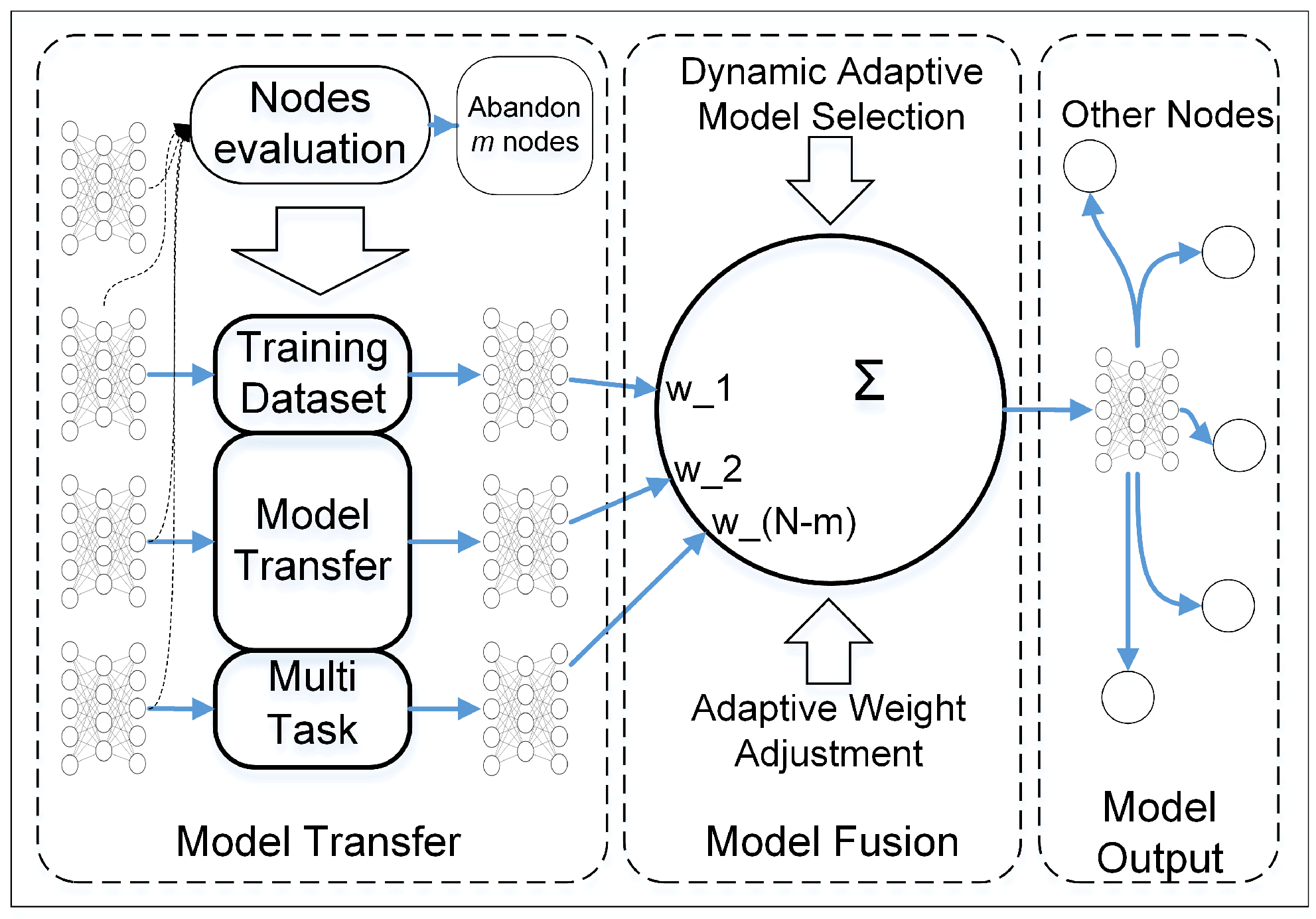
In this study, a P2PNet for fault diagnosis in a large-scale wind turbine cluster and a method belonging to the network are proposed. Each node in P2PNet is equivalent and functional replicable, so a multiple model transfer and dynamic adaptive weight adjustment (MMT-DAWA) model fusion method for tasks in a single node corresponding to a wind turbine gearbox in the cluster is proposed. Each participant in P2PNet saves raw data locally, and only the model parameters are transmitted among nodes. Within a certain node, there are three main steps: model transfer, fusion, and transmission. When the node receives several models from other nodes, it adopts a model transfer based on MTL with EWC constraining model parameters. Then, based on the FL framework, several models are fused by DAWA model fusion with two stages of dynamic adaptive outlier monitoring-based model selection and adaptive weight adjustment-based model fusion. Finally, a better performing model is obtained not only for operation monitoring and fault diagnosis locally but also for transmission to other nodes for iteration and operation. After multi-round iteration and optimization, a state of collaborative intelligence is achieved, where the model performance is better than that of single machine intelligence.
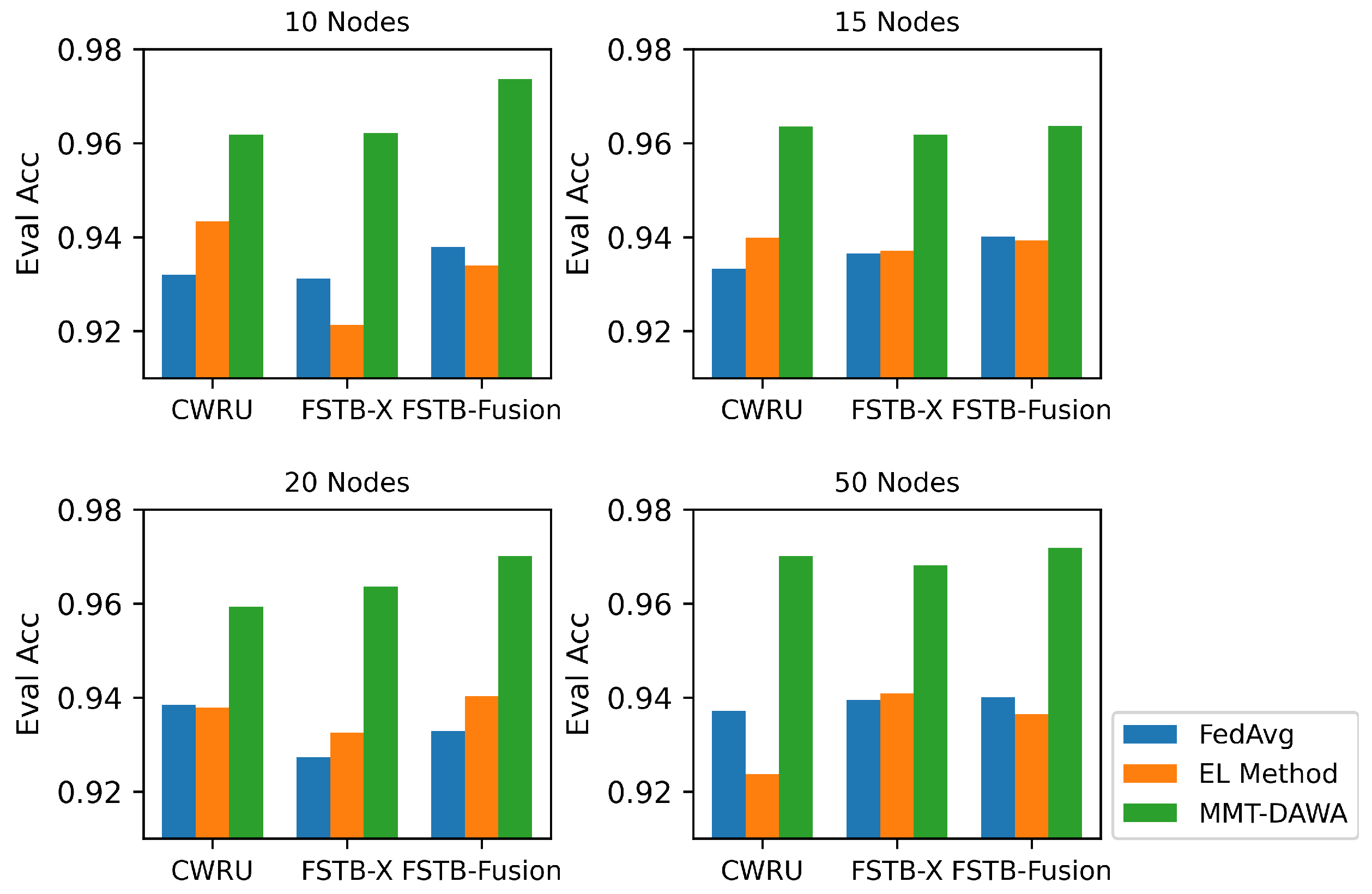
Experiments show the effectiveness and superiority of the methods proposed in this paper. Under any numbers of nodes, the performance of collaborative intelligence is always better than that of single machine intelligence. In any case of the experiment setting, the proposed method performs better than traditional federated average algorithm and ensemble learning-based voting methods for the corresponding tasks.
Therefore, the method proposed in this study is valid in terms of its effectiveness and superiority. This provides a specfic solution to the problems of poor performance of the fault diagnosis model when machine data are insufficient and the data management has obstacles in large-scale turbine clusters. Comparing with similar solutions, the proposed method performs better in terms of the information processing abilitity to deal with data management-based fault diagnosis in a wind turbine cluster. It is also a guidance for other types of machine clusters to implement fault diagnosis.
The future research direction is to combine the algorithm in this study with the comprehensive model transfer and model fusion of various kinds of multimodal signals, striving to understand the operation status of the wind turbines in an all-around way and providing reasonable fault diagnosis results and feasible maintenance schemes.

Author Contributions

Conceptualization, W.Y. and G.Y.; methodology, W.Y.; software, W.Y.; investigation, W.Y.; resources, G.Y.; data curation, W.Y.; writing—original draft preparation, W.Y.; writing—review and editing, W.Y. and G.Y.; visualization, W.Y.; supervision, G.Y.; project administration, G.Y. All authors have read and agreed to the published version of the manuscript.

Funding

This research received no external funding.

Institutional Review Board Statement

Not applicable.

Informed Consent Statement

Not applicable.

Data Availability Statement

Not applicable.

Acknowledgments

The authors would like to thank CWTU for the open-source bearing data for the experiments in this work.

Conflicts of Interest

The authors declare no conflict of interest.

References

  1. Yu, J.; Lv, J. Weak fault feature extraction of rolling bearings using local mean decomposition-based multilayer hybrid denoising. IEEE Trans. Instrum. Meas. 2017, 66, 3148–3159. [Google Scholar] [CrossRef]
  2. Chen, H.; Jiang, B. A review of fault detection and diagnosis for the traction system in high-speed trains. IEEE Trans. Intell. Transp. Syst. 2019, 21, 450–465. [Google Scholar] [CrossRef]
  3. Yang, S.; Yang, P.; Yu, H.; Bai, J.; Feng, W.; Su, Y.; Si, Y. A 2DCNN-RF Model for Offshore Wind Turbine High-Speed Bearing-Fault Diagnosis under Noisy Environment. Energies 2022, 15, 3340. [Google Scholar] [CrossRef]
  4. Jadidi, S.; Badihi, H.; Zhang, Y. Fault-Tolerant Cooperative Control of Large-Scale Wind Farms and Wind Farm Clusters. Energies 2021, 14, 7436. [Google Scholar] [CrossRef]
  5. Imani, M.B.; Heydarzadeh, M.; Khan, L.; Nourani, M. A scalable spark-based fault diagnosis platform for gearbox fault diagnosis in wind farms. In Proceedings of the 2017 IEEE International Conference on Information Reuse and Integration (IRI), San Diego, CA, USA, 4–6 August 2017; pp. 100–107. [Google Scholar]
  6. Jian, C.; Ao, Y. Industrial fault diagnosis based on diverse variable weighted ensemble learning. J. Manuf. Syst. 2022, 62, 718–735. [Google Scholar] [CrossRef]
  7. Kumar, M.P.; Tang, C.J.; Chen, K.C.J. Composite Fault Diagnosis of Rotating Machinery With Collaborative Learning. In Proceedings of the 2022 International Symposium on VLSI Design, Automation and Test (VLSI-DAT), Hsinchu, Taiwan, China, 18–21 April 2022; pp. 1–4. [Google Scholar]
  8. Guo, Q.; Li, Y.; Song, Y.; Wang, D.; Chen, W. Intelligent fault diagnosis method based on full 1-D convolutional generative adversarial network. IEEE Trans. Ind. Inform. 2019, 16, 2044–2053. [Google Scholar] [CrossRef]
  9. Cai, W.; Zhang, Q.; Cui, J. A Novel Fault Diagnosis Method for Denoising Autoencoder Assisted by Digital Twin. Comput. Intell. Neurosci. 2022, 2022, 5077134. [Google Scholar] [CrossRef]
  10. He, Z.; Shao, H.; Wang, P.; Lin, J.J.; Cheng, J.; Yang, Y. Deep transfer multi-wavelet auto-encoder for intelligent fault diagnosis of gearbox with few target training samples. Knowl.-Based Syst. 2020, 191, 105313. [Google Scholar] [CrossRef]
  11. Qian, C.; Zhu, J.; Shen, Y.; Jiang, Q.; Zhang, Q. Deep Transfer Learning in Mechanical Intelligent Fault Diagnosis: Application and Challenge. Neural Process. Lett. 2022, 54, 2509–2531. [Google Scholar] [CrossRef]
  12. Hussain, M.; Al-Aqrabi, H.; Hill, R. Statistical Analysis and Development of an Ensemble-Based Machine Learning Model for Photovoltaic Fault Detection. Energies 2022, 15, 5492. [Google Scholar] [CrossRef]
  13. Wang, R.; Jiang, H.; Li, Z.; Liu, Y. A Deep Ensemble Learning Model for Rolling Bearing Fault Diagnosis. In Proceedings of the 2022 IEEE International Conference on Prognostics and Health Management (ICPHM), Detroit, MI, USA, 6–8 June 2022; pp. 133–136. [Google Scholar]
  14. Wang, S.; Zhang, Y. Multi-Level Federated Network Based on Interpretable Indicators for Ship Rolling Bearing Fault Diagnosis. J. Mar. Sci. Eng. 2022, 10, 743. [Google Scholar] [CrossRef]
  15. Chen, J.; Li, J.; Huang, R.; Yue, K.; Chen, Z.; Li, W. Federated Transfer Learning for Bearing Fault Diagnosis with Discrepancy-Based Weighted Federated Averaging. IEEE Trans. Instrum. Meas. 2022, 71, 1–11. [Google Scholar] [CrossRef]
  16. Mickulicz, N.D.; Narasimhan, P. Performance-Aware Wi-Fi Problem Diagnosis and Mitigation through Peer-to-Peer Data Sharing. In Proceedings of the 2020 50th Annual IEEE-IFIP International Conference on Dependable Systems and Networks-Supplemental Volume (DSN-S), Valencia, Spain, 29 June–2 July 2020; pp. 29–32. [Google Scholar]
  17. Stetco, A.; Dinmohammadi, F.; Zhao, X.; Robu, V.; Flynn, D.; Barnes, M.; Keane, J.; Nenadic, G. Machine learning methods for wind turbine condition monitoring: A review. Renew. Energy 2019, 133, 620–635. [Google Scholar] [CrossRef]
  18. Meyer, A. Vibration Fault Diagnosis in Wind Turbines Based on Automated Feature Learning. Energies 2022, 15, 1514. [Google Scholar] [CrossRef]
  19. Chen, X.; Yang, Y.; Cui, Z.; Shen, J. Vibration fault diagnosis of wind turbines based on variational mode decomposition and energy entropy. Energy 2019, 174, 1100–1109. [Google Scholar] [CrossRef]
  20. Salameh, J.P.; Cauet, S.; Etien, E.; Sakout, A.; Rambault, L. Gearbox condition monitoring in wind turbines: A review. Mech. Syst. Signal Process. 2018, 111, 251–264. [Google Scholar] [CrossRef]
  21. Lei, Y.; Yang, B.; Jiang, X.; Jia, F.; Li, N.; Nandi, A.K. Applications of machine learning to machine fault diagnosis: A review and roadmap. Mech. Syst. Signal Process. 2020, 138, 106587. [Google Scholar] [CrossRef]
  22. Liu, X.; Guo, H.; Liu, Y. One-Shot Fault Diagnosis of Wind Turbines Based on Meta-Analogical Momentum Contrast Learning. Energies 2022, 15, 3133. [Google Scholar] [CrossRef]
  23. Zhao, R.; Yan, R.; Chen, Z.; Mao, K.; Wang, P.; Gao, R.X. Deep learning and its applications to machine health monitoring. Mech. Syst. Signal Process. 2019, 115, 213–237. [Google Scholar] [CrossRef]
  24. Xia, M.; Li, T.; Xu, L.; Liu, L.; De Silva, C.W. Fault diagnosis for rotating machinery using multiple sensors and convolutional neural networks. IEEE/ASME Trans. Mechatron. 2017, 23, 101–110. [Google Scholar] [CrossRef]
  25. Lei, J.; Liu, C.; Jiang, D. Fault diagnosis of wind turbine based on Long Short-term memory networks. Renew. Energy 2019, 133, 422–432. [Google Scholar] [CrossRef]
  26. Wen, L.; Gao, L.; Li, X. A new deep transfer learning based on sparse auto-encoder for fault diagnosis. IEEE Trans. Syst. Man Cybern. Syst. 2017, 49, 136–144. [Google Scholar] [CrossRef]
  27. Qu, F.; Liu, J.; Ma, Y.; Zang, D.; Fu, M. A novel wind turbine data imputation method with multiple optimizations based on GANs. Mech. Syst. Signal Process. 2020, 139, 106610. [Google Scholar] [CrossRef]
  28. Li, X.; Zhang, W.; Ma, H.; Luo, Z.; Li, X. Partial transfer learning in machinery cross-domain fault diagnostics using class-weighted adversarial networks. Neural Netw. 2020, 129, 313–322. [Google Scholar] [CrossRef]
  29. LeCun, Y.; Kavukcuoglu, K.; Farabet, C. Convolutional networks and applications in vision. In Proceedings of the 2010 IEEE International Symposium on Circuits and Systems, Paris, France, 30 May–2 June 2010; pp. 253–256. [Google Scholar]
  30. Li, W.; Huang, R.; Li, J.; Liao, Y.; Chen, Z.; He, G.; Yan, R.; Gryllias, K. A perspective survey on deep transfer learning for fault diagnosis in industrial scenarios: Theories, applications and challenges. Mech. Syst. Signal Process. 2022, 167, 108487. [Google Scholar] [CrossRef]
  31. Yang, B.; Lei, Y.; Jia, F.; Xing, S. An intelligent fault diagnosis approach based on transfer learning from laboratory bearings to locomotive bearings. Mech. Syst. Signal Process. 2019, 122, 692–706. [Google Scholar] [CrossRef]
  32. Li, X.; Hu, Y.; Li, M.; Zheng, J. Fault diagnostics between different type of components: A transfer learning approach. Appl. Soft Comput. 2020, 86, 105950. [Google Scholar] [CrossRef]
  33. Zhou, J.; Zheng, L.Y.; Wang, Y.; Gogu, C. A multistage deep transfer learning method for machinery fault diagnostics across diverse working conditions and devices. IEEE Access 2020, 8, 80879–80898. [Google Scholar] [CrossRef]
  34. Li, X.; Zhang, W.; Ding, Q. Cross-domain fault diagnosis of rolling element bearings using deep generative neural networks. IEEE Trans. Ind. Electron. 2018, 66, 5525–5534. [Google Scholar] [CrossRef]
  35. Xia, B.; Wang, K.; Xu, A.; Zeng, P.; Yang, N.; Li, B. Intelligent Fault Diagnosis for Bearings of Industrial Robot Joints Under Varying Working Conditions Based on Deep Adversarial Domain Adaptation. IEEE Trans. Instrum. Meas. 2022, 71, 1–13. [Google Scholar] [CrossRef]
  36. Liu, X.; Liu, Z.; Wang, G.; Cai, Z.; Zhang, H. Ensemble transfer learning algorithm. IEEE Access 2017, 6, 2389–2396. [Google Scholar] [CrossRef]
  37. Shao, H.; Jiang, H.; Lin, Y.; Li, X. A novel method for intelligent fault diagnosis of rolling bearings using ensemble deep auto-encoders. Mech. Syst. Signal Process. 2018, 102, 278–297. [Google Scholar] [CrossRef]
  38. Wang, Z.Y.; Lu, C.; Zhou, B. Fault diagnosis for rotary machinery with selective ensemble neural networks. Mech. Syst. Signal Process. 2018, 113, 112–130. [Google Scholar] [CrossRef]
  39. Wang, M.; Ge, Q.; Jiang, H.; Yao, G. Wear fault diagnosis of aeroengines based on broad learning system and ensemble learning. Energies 2019, 12, 4750. [Google Scholar] [CrossRef] [Green Version]
  40. Zhang, X.; Huang, T.; Wu, B.; Hu, Y.; Huang, S.; Zhou, Q.; Zhang, X. Multi-model ensemble deep learning method for intelligent fault diagnosis with high-dimensional samples. Front. Mech. Eng. 2021, 16, 340–352. [Google Scholar] [CrossRef]
  41. Li, Z.; Li, Z.; Li, Y.; Tao, J.; Mao, Q.; Zhang, X. An intelligent diagnosis method for machine fault based on federated learning. Appl. Sci. 2021, 11, 12117. [Google Scholar] [CrossRef]
  42. Emamian, M.; Eskandari, A.; Aghaei, M.; Nedaei, A.; Sizkouhi, A.M.; Milimonfared, J. Cloud Computing and IoT Based Intelligent Monitoring System for Photovoltaic Plants Using Machine Learning Techniques. Energies 2022, 15, 3014. [Google Scholar] [CrossRef]
  43. Li, Y.; Chen, Y.; Zhu, K.; Bai, C.; Zhang, J. An effective federated learning verification strategy and its applications for fault diagnosis in industrial IOT systems. IEEE Internet Things J. 2022, 9, 16835–16849. [Google Scholar] [CrossRef]
  44. Ning, D.; Yu, J.; Huang, J. An Intelligent Device Fault Diagnosis Method in Industrial Internet of Things. In Proceedings of the 2018 International Symposium in Sensing and Instrumentation in IoT Era (ISSI), Shanghai, China, 6–7 September 2018; pp. 1–6. [Google Scholar]
  45. Yang, Q.; Liu, Y.; Chen, T.; Tong, Y. Federated machine learning: Concept and applications. ACM Trans. Intell. Syst. Technol. TIST 2019, 10, 1–19. [Google Scholar] [CrossRef]
  46. Wang, Q.; Li, Q.; Wang, K.; Wang, H.; Zeng, P. Efficient federated learning for fault diagnosis in industrial cloud-edge computing. Computing 2021, 103, 2319–2337. [Google Scholar] [CrossRef]
  47. Ma, X.; Wen, C.; Wen, T. An Asynchronous and Real-Time Update Paradigm of Federated Learning for Fault Diagnosis. IEEE Trans. Ind. Inform. 2021, 17, 8531–8540. [Google Scholar] [CrossRef]
  48. Zhang, J.; Wang, Y.; Zhu, K.; Zhang, Y.; Li, Y. Diagnosis of Interturn Short-Circuit Faults in Permanent Magnet Synchronous Motors Based on Few-Shot Learning Under a Federated Learning Framework. IEEE Trans. Ind. Inform. 2021, 17, 8495–8504. [Google Scholar] [CrossRef]
  49. Kevin, I.; Wang, K.; Zhou, X.; Liang, W.; Yan, Z.; She, J. Federated Transfer Learning Based Cross-Domain Prediction for Smart Manufacturing. IEEE Trans. Ind. Inform. 2021, 18, 4088–4096. [Google Scholar] [CrossRef]
  50. Zhang, W.; Li, X. Federated transfer learning for intelligent fault diagnostics using deep adversarial networks with data privacy. IEEE/ASME Trans. Mechatron. 2021, 27, 430–439. [Google Scholar] [CrossRef]
  51. Chen, H.; Chai, Z.; Jiang, B.; Huang, B. Data-driven fault detection for dynamic systems with performance degradation: A unified transfer learning framework. IEEE Trans. Instrum. Meas. 2020, 70, 1–12. [Google Scholar] [CrossRef]
  52. Xu, B.; Wang, N.; Chen, T.; Li, M. Empirical evaluation of rectified activations in convolutional network. arXiv 2015, arXiv:1505.00853. [Google Scholar]
  53. He, K.; Zhang, X.; Ren, S.; Sun, J. Delving deep into rectifiers: Surpassing human-level performance on imagenet classification. In Proceedings of the IEEE International Conference on Computer Vision, Santiago, Chile, 11–18 December 2015; pp. 1026–1034. [Google Scholar]
  54. Pan, S.J.; Yang, Q. A survey on transfer learning. IEEE Trans. Knowl. Data Eng. 2009, 22, 1345–1359. [Google Scholar] [CrossRef]
  55. Vandenhende, S.; Georgoulis, S.; Van Gansbeke, W.; Proesmans, M.; Dai, D.; Van Gool, L. Multi-task learning for dense prediction tasks: A survey. IEEE Trans. Pattern Anal. Mach. Intell. 2021, 44, 3614–3633. [Google Scholar] [CrossRef]
  56. Smith, W.A.; Randall, R.B. Rolling element bearing diagnostics using the Case Western Reserve University data: A benchmark study. Mech. Syst. Signal Process. 2015, 64, 100–131. [Google Scholar] [CrossRef]
  57. Dogo, E.; Afolabi, O.; Nwulu, N.; Twala, B.; Aigbavboa, C. A comparative analysis of gradient descent-based optimization algorithms on convolutional neural networks. In Proceedings of the 2018 international conference on computational techniques, electronics and mechanical systems (CTEMS), Belgaum, India, 21–22 December 2018; pp. 92–99. [Google Scholar]
  58. Van der Maaten, L.; Hinton, G. Visualizing data using t-SNE. J. Mach. Learn. Res. 2008, 9, 2579–2605. [Google Scholar]
  59. McMahan, B.; Moore, E.; Ramage, D.; Hampson, S.; Arcas, B.A.y. Communication-efficient learning of deep networks from decentralized data. Artif. Intell. Stat. Proc. Machine Learn. Res. 2017, 54, 1273–1282. [Google Scholar]
Figure 1. Fault diagnosis framework for wind turbine cluster based on a peer-to-peer network.
Machines 10 00972 g001
Figure 2. Information process in a single node with three main segments: model transfer, model fusion, and model output.
Machines 10 00972 g002
Figure 3. Basic structure of a shallow and small convolutional neural network (CNN).
Machines 10 00972 g003
Figure 4. Transfer learning in cluster networks, where multi-task learning is introduced.
Machines 10 00972 g004
Figure 5. Model and network process: dynamic adaptive outlier monitoring-based model selection and weight adjustment-based model fusion.
Machines 10 00972 g005
Figure 6. Evaluating indicator and result of polynomial fitting. Sub-figure (a) is the variation between mean square error and polynomial order, sub-figure (b) is between R2-Score and polynomial order, and sub-figure (c) is between ε and the number of participants in a cluster.
Machines 10 00972 g006
Figure 7. Bearing experimental platforms. Sub-figure (a) indicates the experimental platform of Case Western Reserve University and sub-figure (b) is the fault signal testing bed.
Machines 10 00972 g007
Figure 8. Data samples with 2000 rpm in speed and 10 V in brake voltage of FSTB Direction X. “H” indicates “Heavy”, “L” indicates “Light”, and “M” indicates “Moderate”, which represent different fault degrees. “Outer”, “Inner”, and “Ball” represent different fault position, respectively. “Normal” indicates no fault.
Machines 10 00972 g008
Figure 9. Influence of the hyperparameters on the results. Sub-figure (a) indicates the global epoch and transfer epoch, and sub-figure (b) corresponds to the data sample length and number.
Machines 10 00972 g009
Figure 10. Variation of model accuracy under different combinations of λ and β .
Machines 10 00972 g010
Figure 11. Evaluating accuracy of the method proposed in the peer-to-peer network with different datasets and various node numbers. Different bars represent different numbers of models in a cluster. The last “Sgl” shows only one model in a single machine intelligence mode.
Machines 10 00972 g011
Figure 12. T-distributed stochastic neighbor embedding visualization of the convolutional neural network features and layers in Node 0.
Machines 10 00972 g012
Figure 13. Confusion matrix of the fault diagnosis model in node 0.
Machines 10 00972 g013
Figure 14. Evaluating accuracy comparison among federated average (FedAvg), ensemble learning voting (EL Method), and multi-model transfer and dynamic adaptive weight adjustment (MMT-DAWA) with node numbers varying among 10, 15, 20, and 50.
Machines 10 00972 g014
Table 1. Comparison of statistical properties between real data and generated data. The comparing items include the maximum, minimum, range, mean, median and standard deviation.
DataMaxMinRangeMeanMedianSTD
Generated0.99991 × 10 8 0.99990.49980.50050.2887
True0.66790.00340.66450.18790.13930.1405
Table 2. Basic hyperparameters configuration.
HyperparameterValueHyperparameterValue
Global Epoch30Sample Length1024
Transfer Epoch100Sample Number300
Transfer Batchsize16 λ 0.95
Fusion Batchsize64 β 1
Learning Rate0.0001 ε 0.672
Node Number10 α 0.954
Momentum0.99--
Table 3. Evaluating accuracy in various methods comparison. The C, FX, and FF at the former positions represent the dataset of CWRU, FSTB Direction X, and FSTB Fusion. The FA, EL, and M at the latter positions represent the method of FedAvg, EL Method, and MMT-DAWA.
NodesC-FAFX-FAFF-FAC-ELFX-ELFF-ELC-MFX-MFF-M
1093.2093.1193.7994.3392.1393.4096.1796.2297.36
1593.3293.6594.0193.9893.7193.9396.3596.1796.36
2093.8592.7393.2993.7993.2694.0395.9396.3697.01
5093.7293.9594.0192.3794.0993.6597.0296.8197.19
Table 4. Experimental verification among the four types of methods.
Group No.BaseMTLDAWAProposed
MaxMinMeanMedian
084.0294.6284.4488.5289.1488.5397.74
179.0193.6985.4289.2188.9890.5796.58
285.2893.9884.9688.3288.5889.8598.56
378.6294.0883.0187.4887.3290.2497.27
482.2091.8782.2887.1288.5192.3699.13
581.8693.8583.4989.9290.1291.5898.82
683.3594.6087.2889.6188.5793.5696.35
784.7991.7482.3288.7486.7589.6197.49
Publisher’s Note: MDPI stays neutral with regard to jurisdictional claims in published maps and institutional affiliations.

