
Machine Learning in CNC Machining: Best Practices
Department of Mechanical and Materials Engineering, Queen’s University, Kingston, ON K7L 3N6, Canada
*
Author to whom correspondence should be addressed.
Machines 2022, 10(12), 1233; https://doi.org/10.3390/machines10121233
Submission received: 26 October 2022
/
Revised: 4 December 2022
/
Accepted: 10 December 2022
/
Published: 16 December 2022
(This article belongs to the Special Issue Safety of Machinery: Design, Monitoring, Manufacturing)
Abstract
:Building machine learning (ML) tools, or systems, for use in manufacturing environments is a challenge that extends far beyond the understanding of the ML algorithm. Yet, these challenges, outside of the algorithm, are less discussed in literature. Therefore, the purpose of this work is to practically illustrate several best practices, and challenges, discovered while building an ML system to detect tool wear in metal CNC machining. Namely, one should focus on the data infrastructure first; begin modeling with simple models; be cognizant of data leakage; use open-source software; and leverage advances in computational power. The ML system developed in this work is built upon classical ML algorithms and is applied to a real-world manufacturing CNC dataset. The best-performing random forest model on the CNC dataset achieves a true positive rate (sensitivity) of 90.3% and a true negative rate (specificity) of 98.3%. The results are suitable for deployment in a production environment and demonstrate the practicality of the classical ML algorithms and techniques used. The system is also tested on the publicly available UC Berkeley milling dataset. All the code is available online so others can reproduce and learn from the results.
1. Introduction
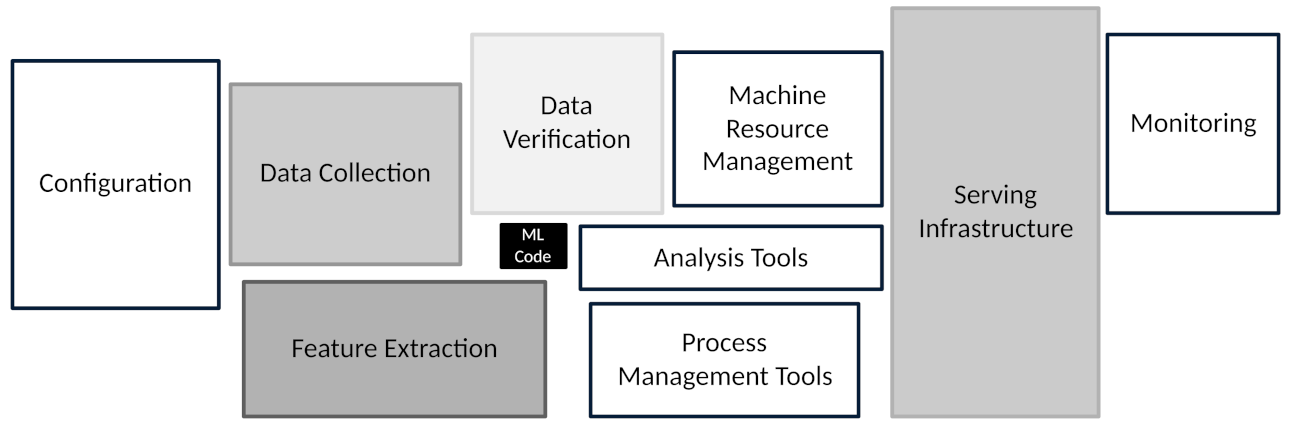
Machine learning (ML) is proliferating throughout society and business. However, much of today’s published ML research is focused on the machine learning algorithm. Yet, as Chip Huyen notes, the machine learning algorithm “is only a small part of an ML system in production” [1]. Building and then deploying ML systems (or applications) into complex real-world environments requires considerable engineering acumen and knowledge that extend far beyond the machine learning code, or algorithm, as shown in Figure 1 [2].
Fortunately, there is a growing recognition of the challenges in building and deploying ML systems, as discussed below and highlighted in Table 1. As such, individuals, from both industry and academia, have begun sharing their learnings, failures, and best practices [1,2,3,4,5,6]. The sharing of this knowledge is invaluable for those who seek to practically use ML in their chosen domain.
However, the sharing of these best practices within manufacturing is less numerous. Zhao et al. and Albino et al. both discuss the infrastructure and engineering requirements for building ML systems in manufacturing [8,9]. Williams and Tang articulate a methodology for monitoring data quality within industrial ML systems [10]. Finally, Luckow et al. briefly discuss some best practices they have observed while building ML systems from within the automotive manufacturing industry [11].
Clearly, there are strong benefits to deploying ML systems in manufacturing [12,13]. Therefore, an explicit articulation of best practices, and a discussion of the challenges involved, is beneficial to all engaged at the intersection of manufacturing and machine learning. As such, we have highlighted five best practices, discovered through our research, namely the following:
- 1.
- Focus on the data infrastructure first.
- 2.
- Start with simple models.
- 3.
- Beware of data leakage.
- 4.
- Use open-source software.
- 5.
- Leverage computation.
We draw from a real-world case study, with data provided by an industrial partner, to illustrate these best practices. The application concerns the building of a ML system for tool wear detection on a CNC machine. A data-processing pipeline is constructed which is then used to train classical machine learning models on the CNC data. We frankly discuss the challenges and learnings, and how they relate to the five best practices highlighted above. The machine learning system is also tested on the common UC Berkeley milling dataset [14]. All the code is made publicly available so that others can reproduce the results. However, due to the proprietary nature of the CNC dataset, we have only made the CNC feature dataset publicly available.
Undoubtedly, there are many more “best practices” relevant to deploying machine learning systems with manufacturing. In this work, we share our learnings, failures, and the best practices that were discovered while building ML tools within the important manufacturing domain.
2. Dataset Descriptions
2.1. UC Berkeley Milling Dataset
The UC Berkeley milling data set contains 16 cases of milling tools performing cuts in metal [14]. Six cutting parameters were used in the creation of the data: the metal type (either cast iron or steel), the feed rate (either 0.25 mm/rev or 0.5 mm/rev), and the depth of cut (either 0.75 mm or 1.5 mm). Each case is a combination of the cutting parameters (for example, case one has a depth of cut of 1.5 mm, a feed rate of 0.5 mm/rev, and is performed on cast iron). The cases progress from individual cuts representing the tool when healthy, to degraded, and then worn. There are 165 cuts amongst all 16 cases. There are two additional cuts that are not considered due to data corruption. Table A1, in Appendix A, shows the cutting parameters used for each case.
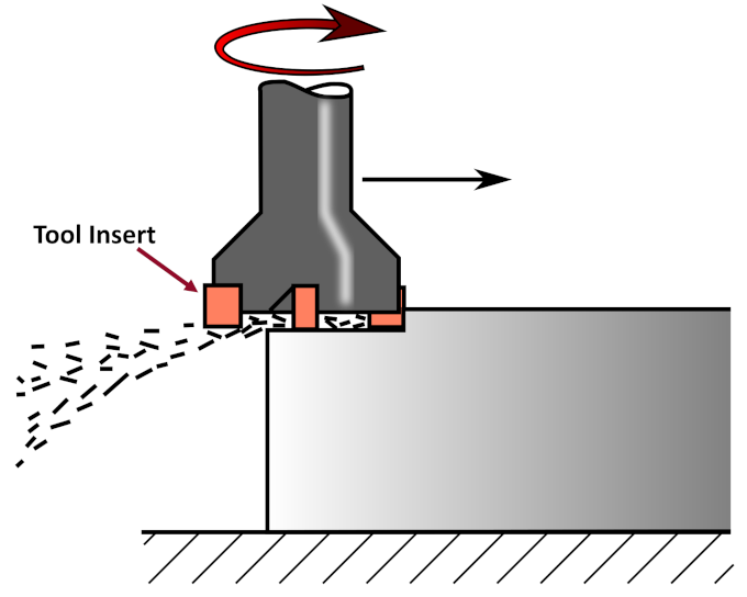
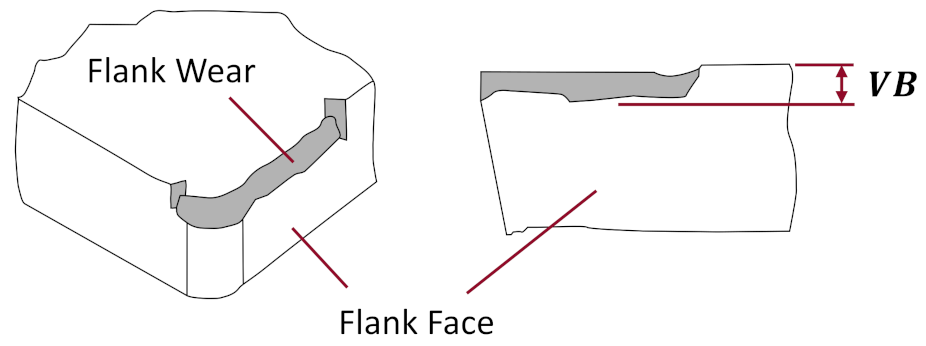
Figure 2 illustrates a milling tool and its cutting inserts working on a piece of metal. A measure of flank wear (VB) on the milling tool inserts was taken for most cuts in the data set. Figure 3 shows the flank wear on a tool insert.
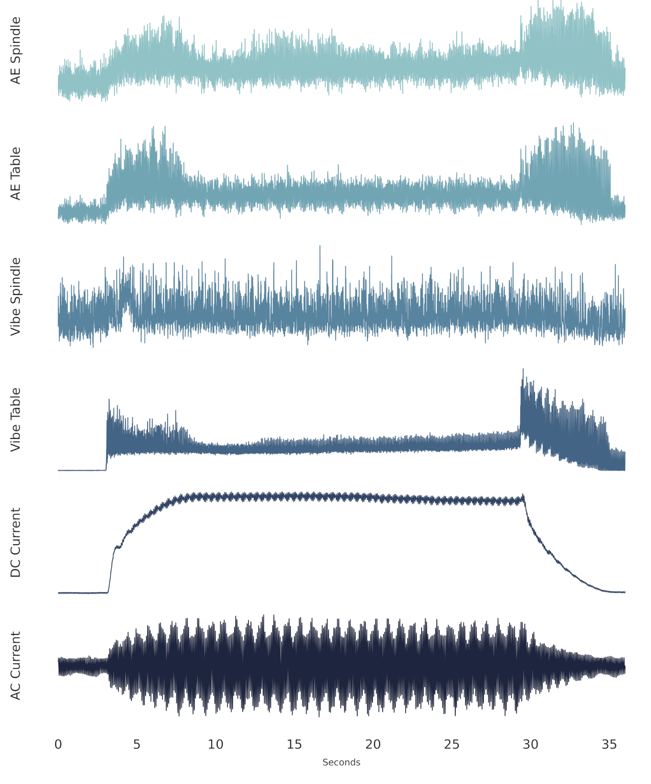
Six signal types were collected during each cut: acoustic emission (AE) signals from the spindle and table; vibration from the spindle and table; and AC/DC current from the spindle motor. The signals were collected at a sampling rate of 250 Hz, and each cut has 9000 sample points, for a total signal length of 36 s. All the cuts were organized in a structured MATLAB array as described by the authors of the dataset. Figure 4 shows a representative sample of a single cut.
Each cut has a region of stable cutting, that is, where the tool is at its desired speed and feed rate, and fully engaged in cutting the metal. For the cut in Figure 4, the stable cutting region begins at approximately 7 s and ends at approximately 29 s when the tool leaves the metal it is machining.
2.2. CNC Industrial Dataset
Industrial CNC data, from a manufacturer involved in the metal machining of small ball-valves, were collected over a period of 27 days. The dataset represents the manufacturing of 5600 parts across a wide range of metal materials and cutting parameters. The dataset was also accompanied by tool change data, annotated by the operator of the CNC machine. These annotations indicated the time the tools were changed, along with the reason for the tool change (either the tool broke, or the tool was changed due to wear).
A variety of tools were used in the manufacturing of the parts. Disposable tool inserts, such as that shown in Figure 3, were used to make the cuts. The roughing tool, and its insert, was changed most often due to wear and thus is the focus of this study.
The CNC data, like the milling data, can also be grouped into different cases. Each case represents a unique roughing tool insert. Of the 35 cases in the dataset, 11 terminated in a worn tool insert as identified by the operator. The remaining cases had the data collection stopped before the insert was worn, or the insert was replaced for another reason, such as breakage.
Spindle motor current was the primary signal collected from the CNC machine. Using motor current within machinery health monitoring (MHM) is widespread and has been shown to be effective in tool condition monitoring [16,17]. In addition, monitoring spindle current is a low-cost and unobtrusive method, and thus ideal for an active industrial environment.
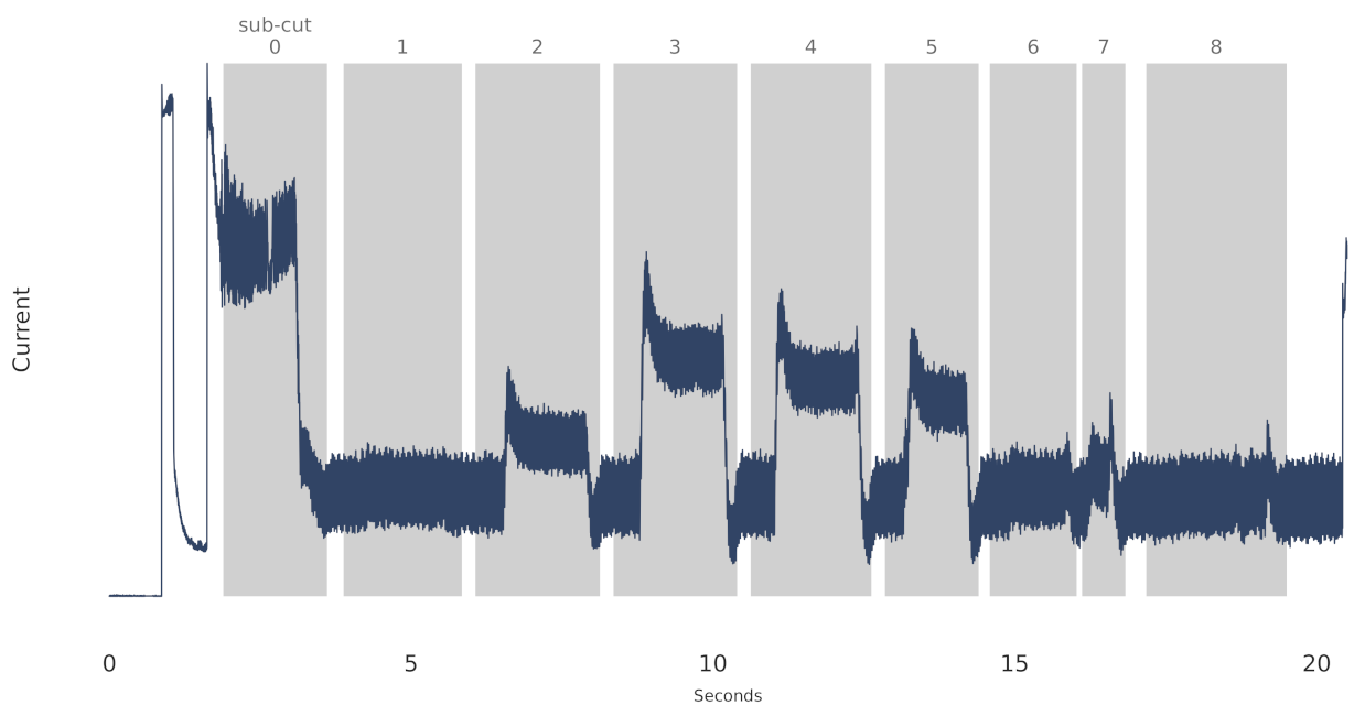
Finally, the data were collected from the CNC machine’s control system using software provided by the equipment manufacturer. For the duration of each cut, the current, the tool being used, and when the tool was engaged in cutting the metal, was recorded. The data were collected at 1000 Hz. Figure 5, below, is an example of one such cut from the roughing tool. The shaded area in the figure represents the approximate time when the tool was cutting the metal. We refer to each shaded area as a sub-cut.
3. Methods
3.1. Milling Data Preprocessing
Each of the 165 cuts from the milling dataset was labeled as healthy, degraded, or failed, according to its health state (amount of wear) at the end of the cut. The labeling schema is shown in Table 2 and follows the labeling strategy of other researchers in the field [18]. For some of the cuts, a flank wear value was not provided. In such a case, a simple interpolation between the nearest cuts, with flank wear values defined, was made.
Next, the stable cutting interval for each cut was selected. The interval varies based on when the tool engages with the metal. Thus, visual inspection was used to select the approximate region of stable cutting.
For each of the 165 cuts, a sliding window of 1024 data points, or approximately 1 s of data, was applied. The stride of the window was set to 64 points as a simple data-augmentation technique. Each windowed sub-cut was then appropriately labeled (either healthy, degraded, or failed). These data preprocessing steps were implemented with the open-source PyPHM package and can be readily reproduced [19].
In total, 9040 sub-cuts were created. Table 2 also demonstrates the percentage of sub-cuts by label. The healthy and degraded labels were merged into a “healthy” class label (with a value of 0) in order to create a binary classification problem.
3.2. CNC Data Preprocessing
As noted in Section 2.2, each part manufactured is made from multiple cuts across different tools. Here, we only considered the roughing tool for further analysis. The roughing tool experienced the most frequent tool changes due to wear.
Each sub-cut, as shown in Figure 5, was extracted and given a unique identifier. The sub-cuts were then labeled either healthy (0) or failed (1). If a tool was changed due to wear, the prior 15 cuts were labeled as failed. Cuts with tool breakage were removed from the dataset. Table 3, below, shows the cut and sub-cut count and the percentage breakdown by label. In total, there were 5503 complete cuts performed by the roughing tool.
3.3. Feature Engineering
Automated feature extraction was performed using the tsfresh open-source library [20]. The case for automated feature extraction continues to grow as computing power becomes more abundant [21]. In addition, the use of an open-source feature extraction library, such as tsfresh, saves time by removing the need to re-implement code for common feature extraction or data-processing techniques.
The tsfresh library comes with a wide variety of time-series feature engineering techniques, and new techniques are regularly being added by the community. The techniques vary from simple statistical measures (e.g., standard deviations) to Fourier analysis (e.g., FFT coefficients). The library has been used for feature engineering across industrial applications. Unterberg et al. utilized tsfresh in an exploratory analysis of tool wear during sheet-metal blanking [22]. Sendlbeck et al. built a machine learning model to predict gear wear rates using the library [23]. Gurav et al. also generated features with tsfresh in their experiments mimicking an industrial water system [24].
In this work, 38 unique feature methods, from tsfresh, were used to generate features. Table 4 lists a selection of these features. In total, 767 features on the CNC dataset were created, and 4530 features, across all six signals, were created on the milling dataset.
After feature engineering, and the splitting of the data into training and testing sets, the features were scaled using the minimum and maximum values from the training set. Alternatively, standard scaling was applied, whereby the mean of a feature, across all samples, was subtracted and then divided by its standard deviation.
3.4. Feature Selection
The large number of features, generated through automated feature extraction, necessitates a method of feature selection. Although it is possible to use all the features for training a machine learning model, it is highly inefficient. Features may be highly correlated with others, and some features will contain minimal informational value. Even more, in a production environment, it is unrealistic to generate hundreds, or thousands, of features for each new sample. This is particularly important if one is interested in real-time prediction.
Two types of feature selection were used in this work. First, and most simply, a certain number of features were selected at random. These features were then used in a random search process (discussed further in Section 4) for the training of machine learning models. Through this process, only the most beneficial features would yield suitable results.
The second type of feature selection leverages the inbuilt selection method within tsfresh. The tsfresh library implements the "FRESH" algorithm, standing for feature extraction based on scalable hypothesis tests. In short, a hypothesis test is conducted for each feature to determine if the feature has relevance in predicting a value. In our case, the predicted value is whether the tool is in a healthy or failed state. Following the hypothesis testing, the features are ranked by p-value, and only those features below a certain p-value are considered useful. The features are then selected randomly. Full details of the FRESH algorithm are detailed in the original paper [20].
Finally, feature selection can only be conducted on the training dataset as opposed to the full dataset. This is done to avoid data leakage, further discussed in Section 6.
3.5. Over and Under-Sampling
Both the CNC and milling datasets are highly imbalanced; that is, there are far more “healthy” samples in the dataset than “failed”. The class imbalance can lead to problems in training machine models when there are not enough examples of the minority (failed) class.
Over- and under-sampling are used to address class imbalance and improve the performance of machine learning trained on imbalanced data. Over-sampling is when examples from the minority class—the failed samples in the CNC and milling datasets—are copied back into the dataset to increase the size of the minority class. Under-sampling is the reverse. In under-sampling, examples from the majority class are removed from the dataset.
Nine different variants of over- and under-sampling were tested on the CNC and milling datasets and were implemented using the imbalanced-learn (https://github.com/scikit-learn-contrib/imbalanced-learn, accessed on 21 July 2022) software package [25]. The variants, with a brief description, are listed in Table 5. Generally, over-sampling was performed, followed by under-sampling, to achieve a relatively balanced dataset. As with the feature selection, the over- and under-sampling was only performed on the training dataset.
3.6. Machine Learning Models
Eight classical machine learning models were tested in the experiments, namely: the Gaussian naïve-Bayes classifier, the logistic regression classifier, the linear ridge regression classifier, the linear stochastic gradient descent (SGD) classifier, the support vector machine (SVM) classifier, the k-nearest-neighbors classifier, the random forest (RF) classifier, and the gradient boosted machines classifier.
The models range from simple, such as the Gaussian naïve-Bayes classifier, to more complex, such as the gradient boosted machines. All these models can be readily implemented on a desktop computer. Further benefits of these models are discussed in Section 6.
These machine learning models are commonplace, and as such, the algorithm details are not covered in this work. All the algorithms, except for gradient boosted machines, were implemented with the scikit-learn machine learning library in Python [33]. The gradient boosted machines were implemented with the Python XGBoost library [34].
4. Experiment
The experiments on the CNC and milling datasets were conducted using the Python programming language. Many open-source software libraries were used, in addition to tsfresh, scikit-learn, and the XGBoost libraries, as listed above. NumPy [35] and SciPy [36] were used for data preprocessing and the calculation of evaluation metrics. Pandas, a tool for manipulating numerical tables, was used for recording results [37]. PyPHM, a library for accessing and preprocessing industrial datasets, was used for downloading and preprocessing the milling dataset [19]. Matplotlib was used for generating figures [38].
The training of the machine learning models in a random search, as described below, was performed on a high-performance computer (HPC). However, training of the models can also be performed on a local desktop computer. To that end, all the code from the experiments is available online. The results can be readily reproduced, either online through GitHub, or by downloading the code to a local computer. The raw CNC data are not available due to their proprietary nature. However, the generated features, as described in Section 3, are available for download.
4.1. Random Search
As noted, a random search was conducted to find the best model, and parameters, for detecting failed tools on the CNC and milling datasets. A random search is seen as better for determining optimal parameters than a more deterministic grid search [39].
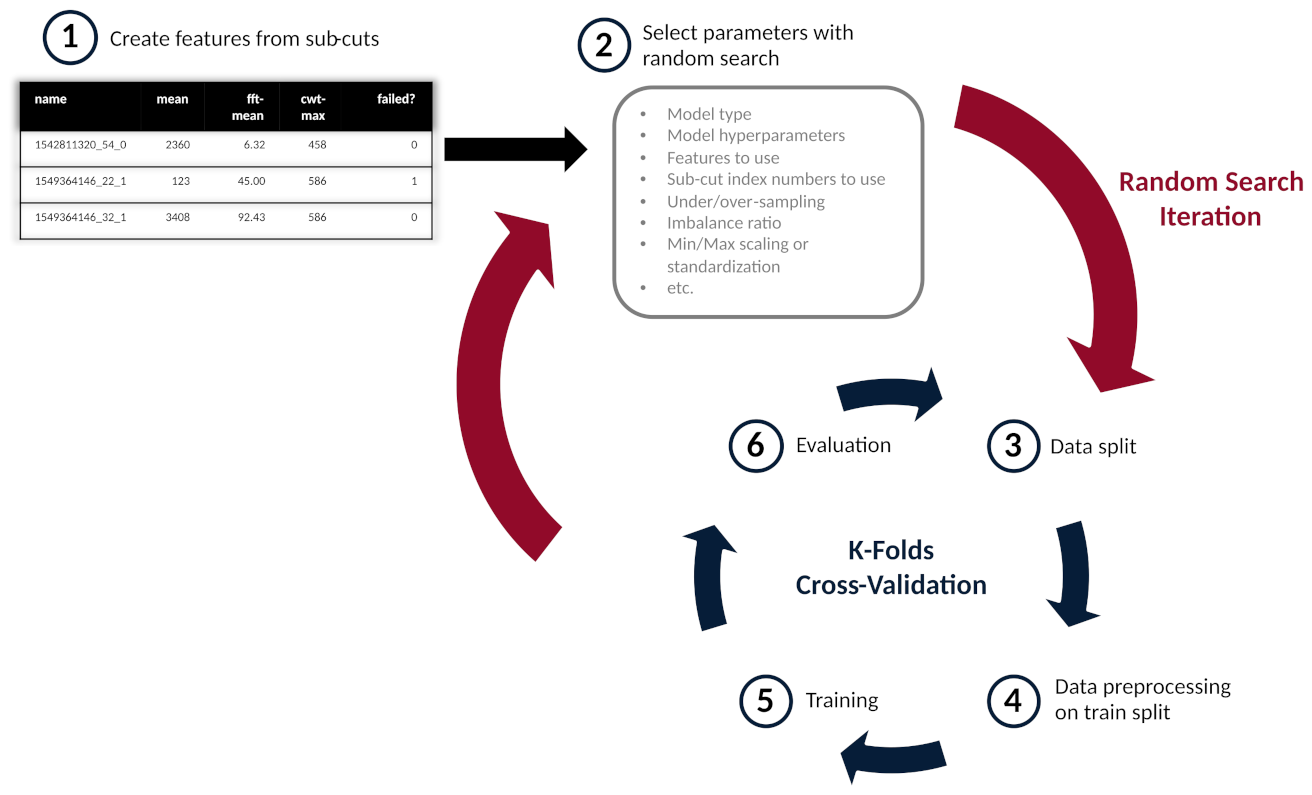
Figure 6 illustrates the random search process on the CNC dataset. After the features are created, as seen in step one, the parameters for a random search iteration are randomly selected. A more complete list of parameters, used for both the CNC and milling datasets, is found in Appendix A. The parameters are then used in a k-folds cross-validation process in order to minimize over-fitting, as seen in steps three through six. Thousands of random search iterations can be run across a wide variety models and parameters.
For the milling dataset, seven folds were used in the cross-validation. To ensure independence between samples in the training and testing sets, the dataset was grouped by case (16 cases total). Stratification was also used to ensure that, in each of the seven folds, at least one case where the tool failed was in the testing set. There were only seven cases that had a tool failure (where the tool was fully worn out), and thus, the maximum number of folds is seven for the milling dataset.
Ten-fold cross validation was used on the CNC dataset. As with the milling dataset, the CNC dataset was grouped by case (35 cases) and stratified.
As discussed above, in Section 3, data preprocessing, such as scaling or over-/under-sampling was conducted after the data was split, as shown in steps three and four. Training of the model was then conducted, using the split and preprocessed data, as shown in step five. Finally, the model could be evaluated, as discussed below.
4.2. Metrics for Evaluation
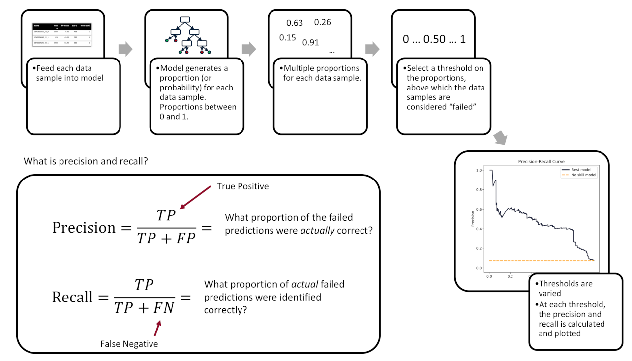
A variety of metrics can be used to evaluate the performance of machine learning models. Measuring the precision–recall area under curve (PR-AUC) is recognized as a suitable metric for binary classification on imbalanced data and, as such, is used in this work [40,41]. In addition, the PR-AUC is agnostic to the final decision threshold, which may be important in applications where the recall is much more important than the precision, or vice versa. Figure 7 illustrates how the precision–recall curve is created.
After each model is trained, in a fold, the PR-AUC is calculated on that fold’s hold-out test data. The PR-AUC scores can then be averaged across each of the folds. In this work, we also rely on the PR-AUC from the worst-performing fold. The worst-performing fold can provide a lower bound of the model’s performance, and as such, provide a more realistic impression of the model’s performance.
5. Results
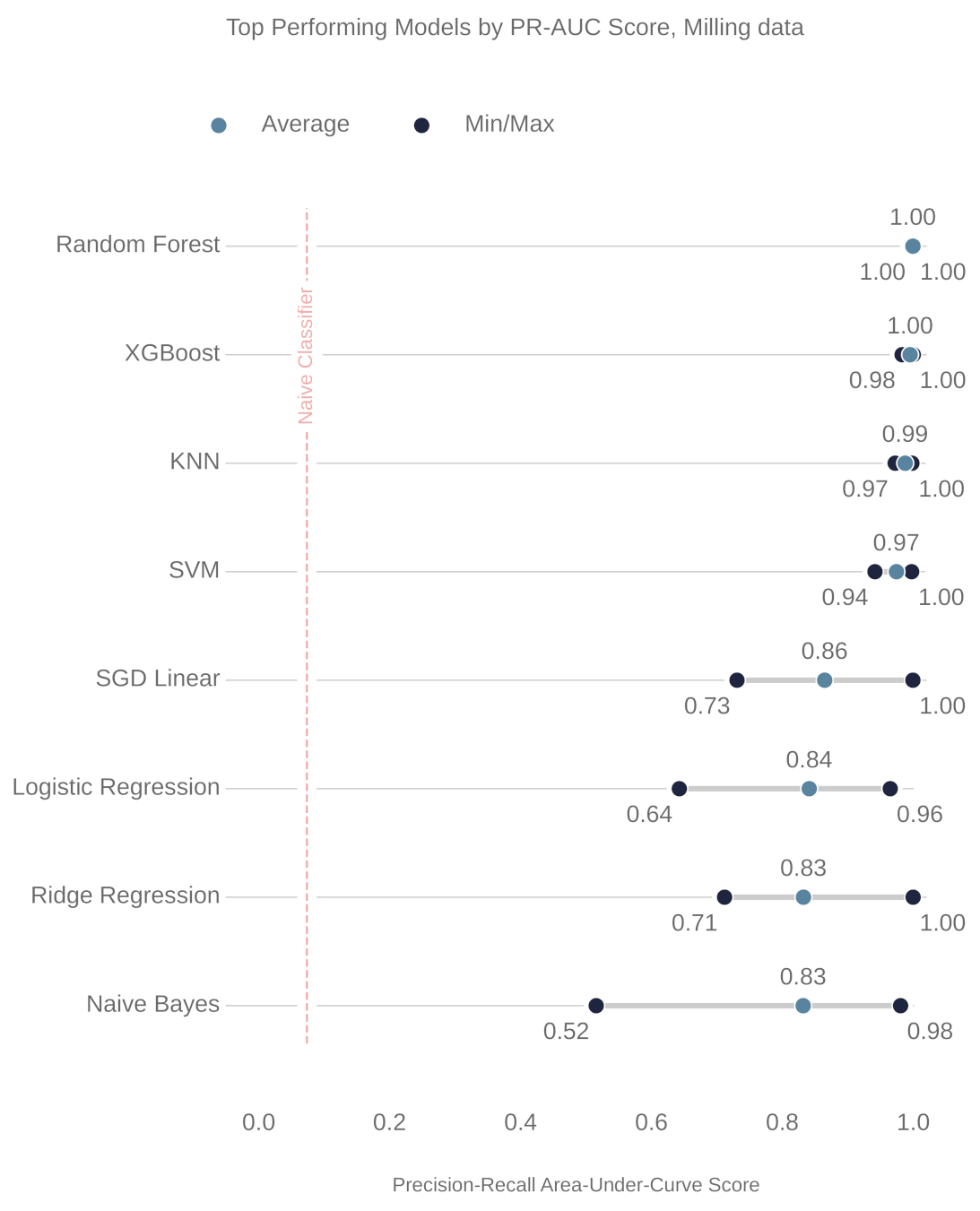
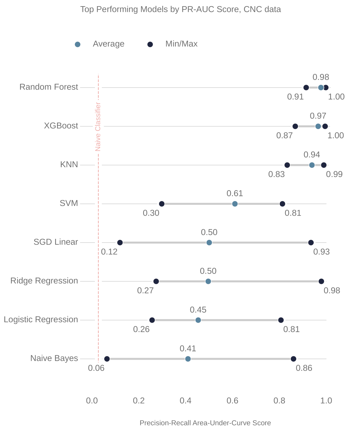
In total, 73,274 and 230,859 models were trained on the milling and CNC datasets, respectively. The top performing models, based on average PR-AUC, were selected and then analyzed further.
Figure 8 and Figure 9 show the ranking of the models for the milling and CNC datasets, respectively. In both cases, the random forest (RF) model outperformed the others. The parameters of these RF models are also shown, below, in Table 6 and Table 7.
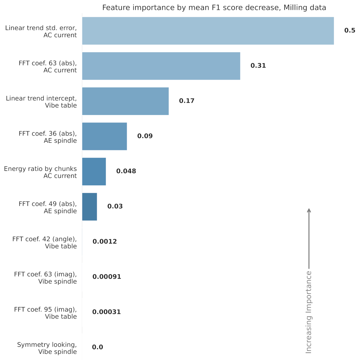
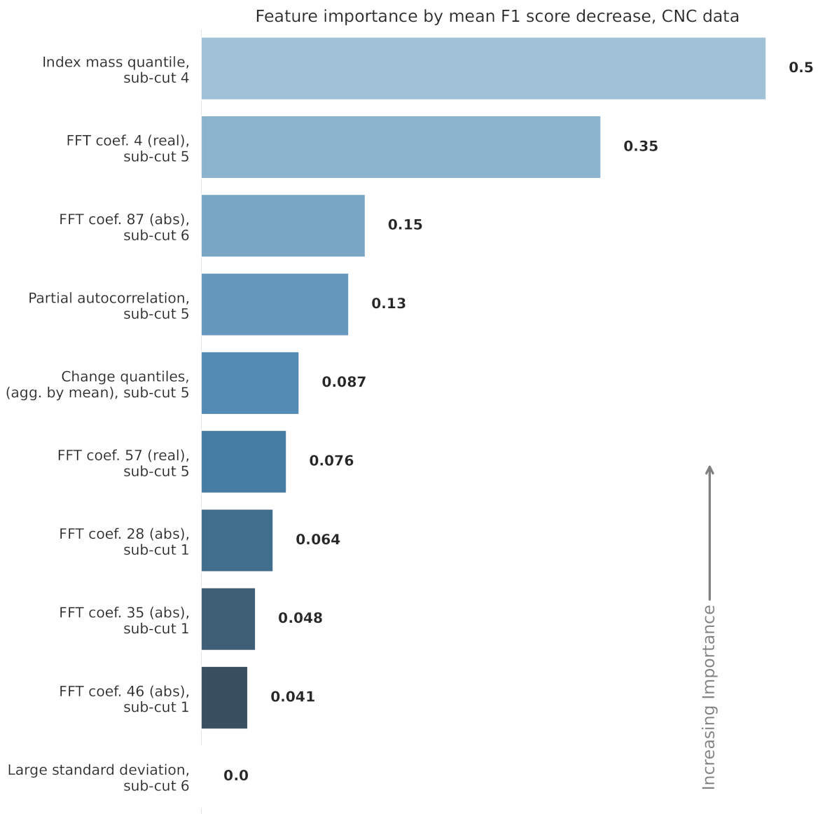
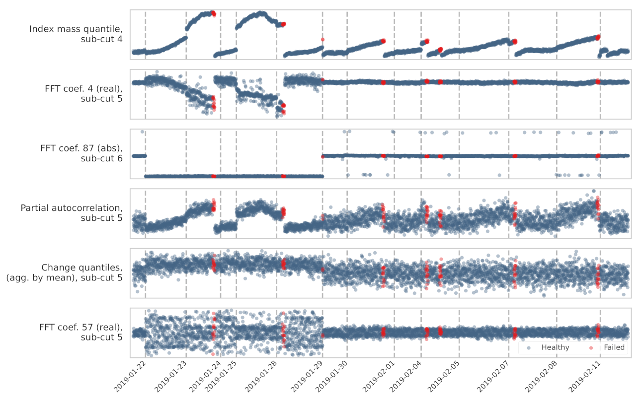
The features used in each RF model are displayed in Figure 10 and Figure 11. The figures also show the relative feature importance by F1 score decrease. Figure 12 shows how the top six features, from the CNC model, trend over time. Clearly, the top ranked feature—the index mass quantile on sub-cut 4—has the strongest trend. The full details, for all the models, are available in Appendix A and in the online repository.
The PR-AUC score is an abstract metric that can be difficult to translate to real-world performance. To provide additional context, we took the worst-performing model in the k-fold and selected the decision threshold that maximized its F1-score. The formula for the F1 score is as follows:
where TP is the number of true positives, FP is the number of false positives, and FN is the number of false negatives.
The true positive rate (sensitivity), the true negative rate (specificity), the false negative rate (miss rate) and false positive rate (fall out), were then calculated with the optimized threshold. Table 7 shows these metrics for the best-performing random forest models, using its worst k-fold.
To further illustrate, consider 1000 parts manufactured on the CNC machine. We know, from Table 3, that approximately 27 (2.7%) of these parts will be made using worn (failed) tools. The RF model will properly classify 24 of the 27 cuts as worn (the true positive rate). Of the 973 parts manufactured using healthy tools, 960 will be properly classified as healthy (the true negative rate).
Analysis, Shortcomings, and Recommendations
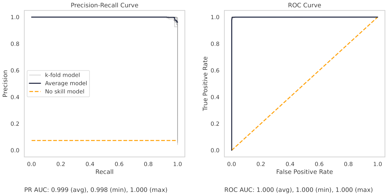
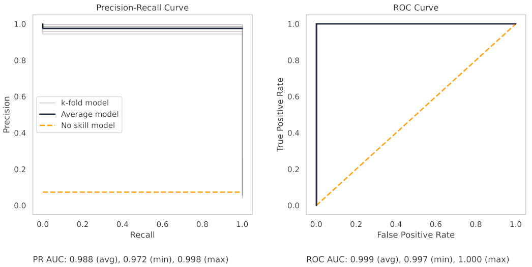
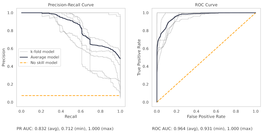
Figure 13 shows the precision–recall (PR) and receiver operating characteristic (ROC) curves for the milling random forest model. These curves help understand the results as shown in the dot plots of Figure 8.
The precision–recall curve, for the milling RF model, shows that all the models on the 7 k-folds give strong results. Each of the curves from the k-folds is pushed to the top right, and as shown in Table 8, even the worst-performing fold achieves a true positive rate of 97.3%.
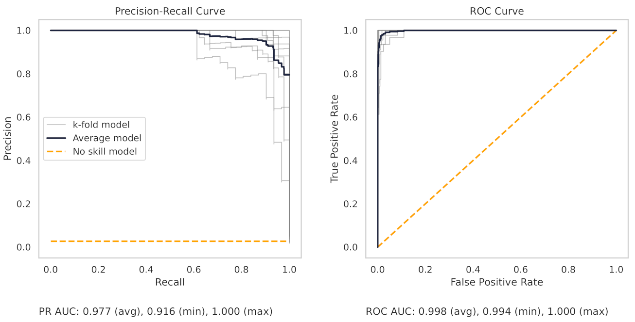
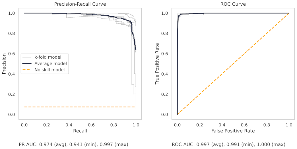
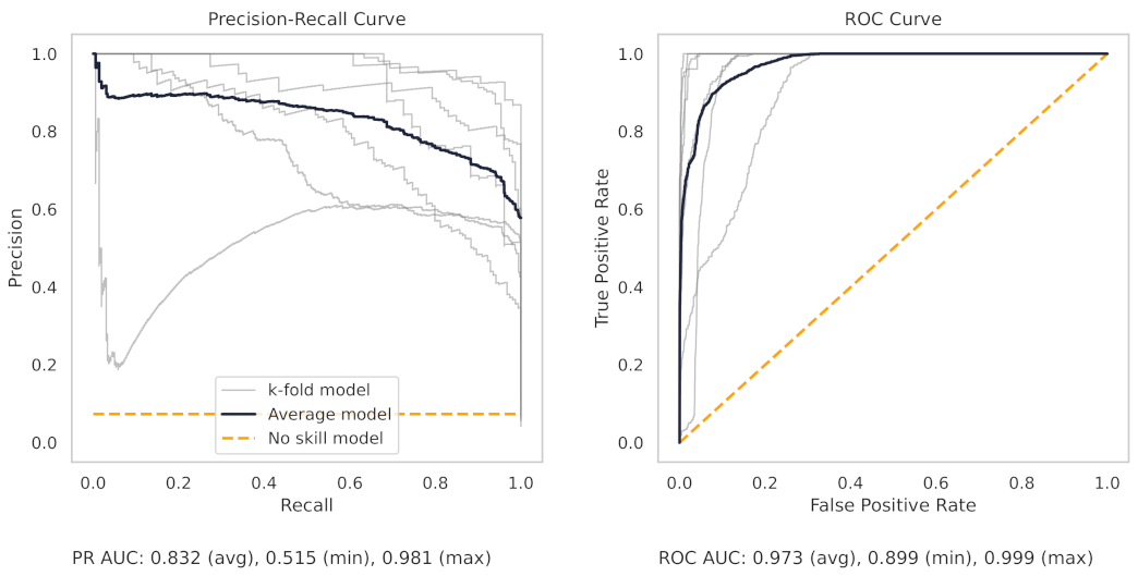
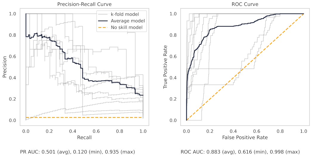
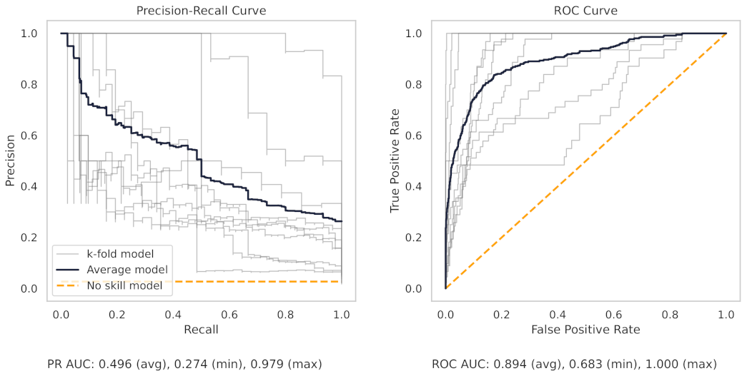
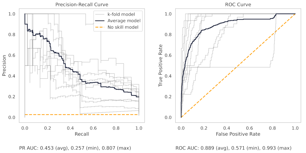
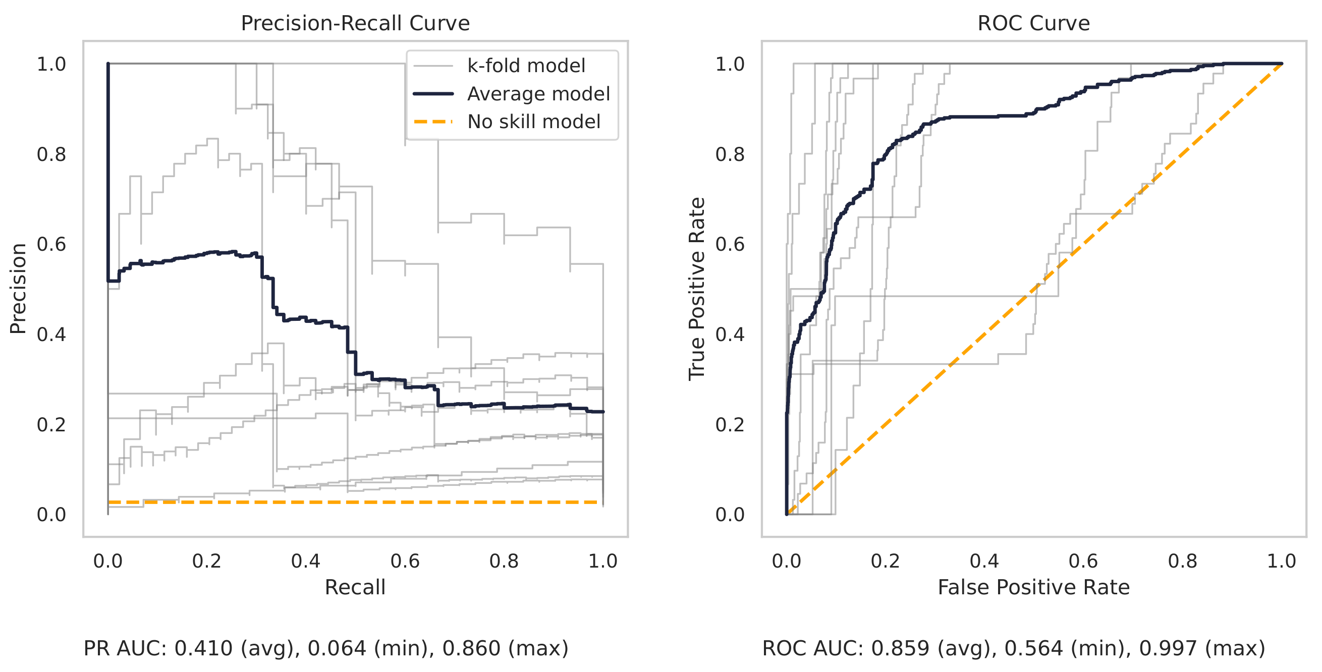
The precision–recall curve from the CNC RF model, as shown in Figure 14, shows greater variance between each trained model in the 10 k-folds. The worst-performing fold obtains a true positive rate of 90.3%.
There are several reasons for the difference in model performance between the milling and CNC datasets. First, each milling sub-cut has six different signals available for use (AC/DC current, vibration from the spindle and table, and acoustic emissions from the spindle and table). Conversely, the CNC model can only use the current from the CNC spindle. The additional signals in the milling data provide increased information for machine learning models to learn from.
Second, the CNC dataset is more complicated. The tools from the CNC machine are changed when the operator notices a degradation in part quality. However, individual operators will have different thresholds, and cues, for changing tools. In addition, there are multiple parts manufactured in the dataset across a wide variety of metals and dimensions. In short, the CNC dataset reflects the conditions of a real-world manufacturing environment with all the “messiness” which that entails. As such, the models trained on the CNC data cannot as easily achieve high results like in the milling dataset.
In contrast, the milling dataset is from a carefully controlled laboratory environment. Consequently, there is less variety between cuts in the milling dataset than in the CNC dataset. The milling dataset is more homogeneous, and the homogeneity allows the models to understand the data distribution and model it more easily.
Third, the milling dataset is smaller than the CNC dataset. The milling dataset has 16 different cases, but only 7 of the cases have a tool that becomes fully worn. The CNC dataset has 35 cases, and of those cases, 11 contain a fully worn tool. The diminished size of the milling dataset, again, allows the models to model the data more easily. As noted by others, many publicly available industrial datasets are small, thus making it difficult for researchers to produce results that are generalizable [42,43]. The UC Berkeley milling dataset suffers from similar problems.
Finally, models trained on small datasets, even with cross validation, can be susceptible to overfitting [44]. Furthermore, high-powered models, such as random forests or gradient boosted machines, are more likely to exhibit a higher variance. The high variance, and overfitting, may give the impression that the model is performing well across all k-folds, but if the data are changed, even slightly, the model performs poorly.
Overall, the CNC dataset is of higher quality than the milling dataset; however, it too suffers from its relatively small size. We posit that similar results could be achieved with only a few cuts from each of the 35 cases. In essence, the marginal benefit of additional cuts in a case rapidly diminishes past the first few since they are all similar. This hypothesis would be of interest for further research.
The results from the CNC dataset are positive, and the lower bound of the model’s performance approaches acceptability. We believe that collecting more data will greatly improve results. Ultimately, the constraint to creating production-ready ML systems is not the type of algorithm, but rather, the lack of data. We further discuss this in the Best Practices section below.
6. Discussion of Best Practices
6.1. Focus on the Data Infrastructure First
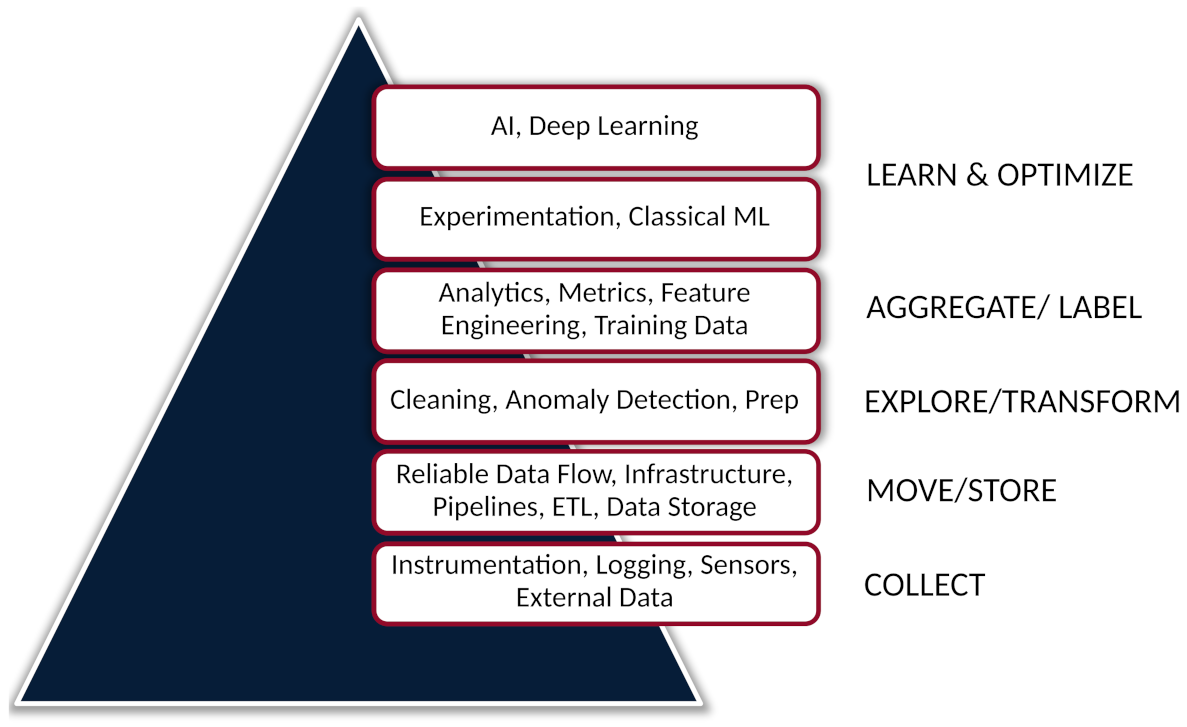
In 2017, Monica Rogati coined the “data science hierarchy of needs” as a play on the well-known Maslow’s hierarchy of needs. Rogati details how the success of a data science project, or ML system, is predicated on a strong data foundation. Having a data infrastructure that can reliably collect, transform, and store data is a prerequisite to upstream tasks, such as data exploration, or machine learning [45]. Figure 15 illustrates this hierarchy.
Within the broader machine learning community, there is a growing acknowledgment of the benefits of a strong data infrastructure. Andrew Ng, a well-known machine learning educator and entrepreneur, has expressed the importance of data infrastructure through his articulation of “data-centric AI” [46]. Within data-centric AI, there is a recognition that outsized benefits can be obtained by improving the data quality first, rather than improving the machine learning model.
As an example of this data-centric approach, consider the OpenAI research team. Recently, they made dramatic advances in speech recognition that have been predicated on the data infrastructure. They used simple heuristics to remove “messy” samples, all the while using off-the-shelf machine learning models. More broadly, the nascent field of machine learning operations (MLOps) has arisen as a means of formalizing the engineering acumen in building ML systems. The data infrastructure is a large part of MLOps [1,7].
In this work, we built the top four tiers of the data science hierarchy pyramid as shown in Figure 15. However, although part of the data infrastructure was built—in the extraction–load–transform (ETL) portion—much of the data infrastructure was outside of the research team’s control. A system to autonomously collect CNC data was not implemented, and as such, far less data were collected than desired. Over a one-year period, data were manually collected for 27 days, which led to the recording of 11 roughing tool failures. Yet, over that same one-year period, there were an additional 79 cases where the roughing tool failed, but no data were collected.
Focusing on the data infrastructure first, the bottom two layers of the pyramid, builds for future success. In a real-world setting, as in manufacturing, the quality of the data will play an outsized role in the success of the ML application being developed. As shown in the next section, even simple models, coupled with good data, can yield excellent results.
6.2. Start with Simple Models
The rise of deep learning has led to much focus, from researchers and industry, on its application in manufacturing. However, as shown in the data science hierarchy of needs, in Figure 15, it is best to start with “simple”, classical ML models. The work presented here relied on these classical ML models, from naïve Bayes to random forests. These models still achieved positive results.
There are several reasons to start with simple models:
- Simple models are straightforward to implement. Modern machine learning packages, such as scikit-learn, or XGBoost, allow the implementation of classical ML models in only several lines of code.
- Simple models require less data than deep learning models.
- Simple models can produce strong results, and in many cases, outperform deep learning models.
- Simple models cost much less to train. Even a random forest model, with several terabytes of data, will only cost a few dollars to retrain on a commercial cloud provider. A large deep learning model, in contrast, may be an order of magnitude more expensive to train.
- Simple models allow for quicker iteration time. This allows users to rapidly “demonstrate [the] practical benefits” of an approach, and subsequently, avoid less-productive approaches [7].
The benefits, and even preference for simple models, are becoming recognized within the research and MLOps communities. Already, in 2006, David Hand noted that “simple methods typically yield performance almost as good as more sophisticated methods” [47]. In fact, more complicated methods can yield over-optimization. Others have shown that tree-based models still outperform deep-learning approaches on tabular [48,49]. Tabular data and tree-based models were both used in this study.
Finally, Shankar et al. recently interviewed 18 machine learning engineers across a variety of companies in an insightful study on operationalizing ML real-world applications. They noted that most of the engineers prefer the use of simple machine-learning algorithms over more complex approaches [7].
6.3. Beware of Data Leakage
Data leakage occurs when information from the target domain (such as the label information on the health state of a tool) is introduced, often unintentionally, into the training dataset. The data leakage produces results that are far too optimistic, and ultimately, useless. Unfortunately, data leakage is difficult to detect for those who are not wary or uneducated. Kaufman et al. summarized the problem succinctly: “In practice, the introduction of this illegitimate information is unintentional, and facilitated by the data collection, aggregation and preparation process. It is usually subtle and indirect, making it very hard to detect and eliminate” [50]. We observed many cases of data leakage in peer-reviewed literature, both from within manufacturing, and more broadly. Data leakage, sadly, is too common across many fields where machine learning is employed [50].
Introducing data leakage into a real-world manufacturing environment will cause the ML system to fail. As such, individuals seeking to employ ML in manufacturing should be cognizant of the common data leakage pitfalls. Here, we explore several of these pitfalls with examples from manufacturing. We adopted the taxonomy from Kapoor et al. and encourage interested readers to view their paper on the topic [51].
- Type 1—Preprocessing on training and test set: Preprocessing techniques, like scaling, normalization, or under-/over-sampling, must only be applied after the dataset has been split into training and testing sets. In our experiment, as noted in Section 3, these preprocessing techniques were performed after the data were split in the k-fold.
- Type 2—Feature selection on training and test set: This form of data leakage occurs when features are selected using the entire dataset at once. By performing feature selection over the entire dataset, additional information will be introduced into the testing set that should not be present. Feature selection should only occur after the train/validation/testing sets are created.
- Type 3—Temporal leakage: Temporal data leakage occurs, on time series data, when the training set includes information from a future event that is to be predicted. As an example, consider case 13 on the milling dataset. Case 13 consists of 15 cuts. Ten of these cuts are when the tool is healthy, and five of the cuts are when the tool is worn. If the cuts from the milling dataset (165 cuts in total) are randomly split into the training and testing sets, then some of the “worn” cuts from case 13 will be in both the training and testing sets. Data leakage will occur, and the results from the experiment will be too optimistic. In our actual experiments, we avoided data leakage by splitting the datasets by case, as opposed to individual cuts.
6.4. Use Open-Source Software
The open-source software movement has consistently produced “category-killing software” across a broad spectrum of fields [52]. Open-source software is ubiquitous in all aspects of computing, from mobile phones, to web browsers, and certainly within machine learning.
Table 9, below, lists several of these open-source software packages that are relevant to building modern ML systems. These software packages are also, predominantly, built using the open-source Python programming language. Python, as a general-purpose language, is easy to understand and is one of the most popular programming languages in existence [53].
The popularity of Python, combined with high-quality open-source software packages, such as those in Table 9, only attracts more data scientists and ML practitioners. Some of these individuals, in the ethos of open-source, improve the software further. Others create instructional content, share their code (such as we have with this research), or simply discuss their challenges with the software. All this creates a dominant network effect; that is, the more users that adopt the open-source Python ML software, the more attractive these tools become to others. Today, Python, and its open-source tools, are dominant within the machine learning space [54].

Table 9.
Several popular open-source machine learning, and related, libraries. All these applications are written in Python.
Table 9.
Several popular open-source machine learning, and related, libraries. All these applications are written in Python.
| Software Name | Description |
|---|---|
| scikit-learn [33] | Various classification, regression, and clustering algorithms. |
| NumPy [35] | Comprehensive mathematical software package. Supports for large multi-dimensional arrays and matrices. |
| PyTorch [55] | Popular deep learning framework. |
| TensorFlow [56] | Popular deep learning framework, originally created by Google. |
Ultimately, using these open-source software packages greatly improves productivity. In our work, we began building our own feature engineering pipeline. However, we soon realized the complexity of that task. As a results, we utilized the open-source tsfresh library to implement the feature engineering pipeline, thus saving countless hours of development time. Individuals looking to build ML systems should consider open-source software first before looking to build their own tools, or using proprietary software.
6.5. Leverage Advances in Computational Power
The rise of deep learning has coincided with the dramatic increase in computation power. Rich Sutton, a prominent machine learning researcher, argued in 2019 that “the biggest lesson that can be read from 70 years of AI research is that general methods that leverage computation are ultimately the most effective, and by a large margin” [57]. Fortunately, it is easier than ever for those building ML systems to tap into the increasing computational power available.
In this work, we utilized a high-performance computer (HPC) to perform an extensive parameter search. Such HPCs are common in academic environments and should be taken advantage of when possible. However, individuals without access to an HPC can also train many classical ML models on regular consumer GPUs. Using GPUs will parallelize the model training process. The XGBoost library allows training on GPUs, which can be integrated into a parameter search. RAPIDS has also developed a suite of open-source libraries for data analysis and training of ML models on GPUs.
Compute power will continue to increase and drop in price. This trend presents opportunities for those who can leverage it. Accelerating data preprocessing, model training, and parameter searches allows teams to iterate faster through ideas, and ultimately, build more effective ML applications.
7. Conclusions and Future Work
Machine learning is becoming more and more integrated into manufacturing environments. In this work we demonstrated an ML system used to predict tool wear on a real-world CNC machine, and on the UC Berkeley milling dataset. The best performing random forest model on the CNC dataset achieved a true positive rate (sensitivity) of 90.3% and a true negative rate (specificity) of 98.3%. Moreover, we used the results to illustrate five best practices, and learnings, that we gained during the construction of the ML system. Namely, one should focus on the data infrastructure first; begin modeling with simple models; be cognizant of data leakage; use open-source software; and leverage advances in computational power.
A productive direction for future work is the further build-out of the data infrastructure. Collecting more data, as noted in Section 5, would improve results and build confidence in the methods developed here. In addition, the ML system should be deployed in the production environment and iterated upon there. Finally, the sharing of the challenges, learnings, and best practices should continue, and we encourage others within manufacturing to do the same. Ultimately, understanding these broader challenges and best practices will enable the efficient use of ML within the manufacturing domain.
Author Contributions
Conceptualization, methodology, software, validation, formal analysis, investigation, data curation, visualization, and writing—original draft preparation, by T.v.H.; writing—review and editing, T.v.H. and C.K.M.; supervision, project administration, and funding acquisition, by C.K.M. All authors have read and agreed to the published version of the manuscript.
Funding
This research was funded by the Natural Sciences and Engineering Research Council of Canada and the Digital Research Alliance of Canada.
Data Availability Statement
The data and code to reproduce the experiments are available at: https://github.com/tvhahn/tspipe.
Conflicts of Interest
The authors declare no conflict of interest.
Appendix A
Appendix A.1. Miscellaneous Tables
Table A1.
The cutting parameters used in the UC Berkeley milling dataset.
| Case | Depth of Cut (mm) | Feed Rate (mm/rev) | Material |
|---|---|---|---|
| 1 | 1.50 | 0.50 | cast iron |
| 2 | 0.75 | 0.50 | cast iron |
| 3 | 0.75 | 0.25 | cast iron |
| 4 | 1.50 | 0.25 | cast iron |
| 5 | 1.50 | 0.50 | steel |
| 6 | 1.50 | 0.25 | steel |
| 7 | 0.75 | 0.25 | steel |
| 8 | 0.75 | 0.50 | steel |
| 9 | 1.50 | 0.50 | cast iron |
| 10 | 1.50 | 0.25 | cast iron |
| 11 | 0.75 | 0.25 | cast iron |
| 12 | 0.75 | 0.50 | cast iron |
| 13 | 0.75 | 0.25 | steel |
| 14 | 0.75 | 0.50 | steel |
| 15 | 1.50 | 0.25 | steel |
| 16 | 1.50 | 0.50 | steel |
Appendix A.2. PR and ROC Curves for the Milling Dataset
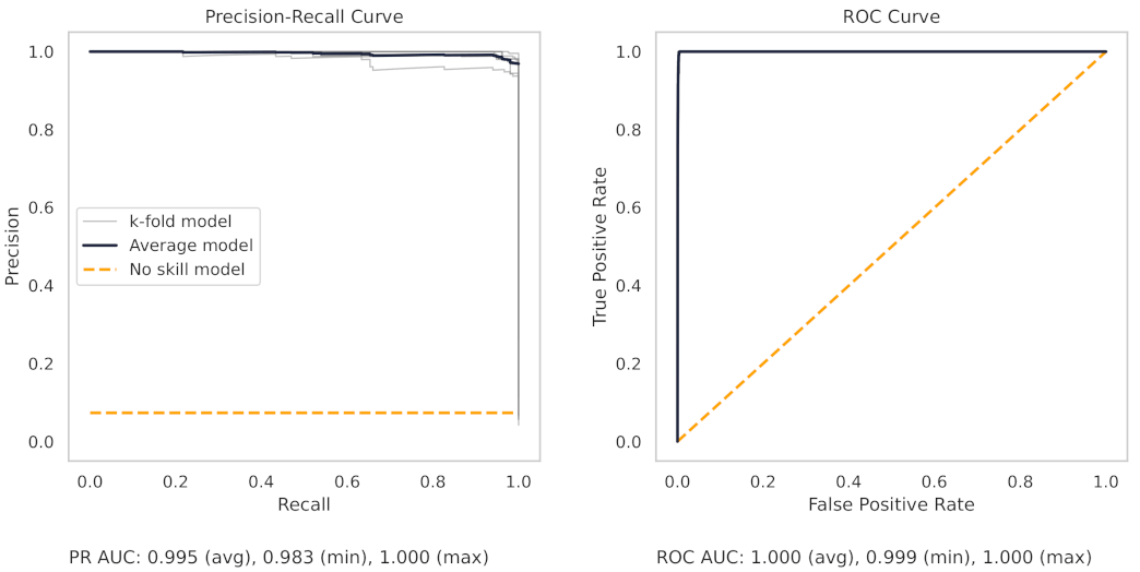
Figure A1.
The PR and ROC curves for the XGBoost milling dataset model.

Figure A2.
The PR and ROC curves for the KNN milling dataset model.

Figure A3.
The PR and ROC curves for the SVM milling dataset model.

Figure A4.
The PR and ROC curves for the SGD linear milling dataset model.

Figure A5.
The PR and ROC curves for the logistic regression milling dataset model.

Figure A6.
The PR and ROC curves for the ridge regression milling dataset model.

Figure A7.
The PR and ROC curves for the Naïve Bayes milling dataset model.

Appendix A.3. PR and ROC Curves for the CNC Dataset
Figure A8.
The PR and ROC curves for the XGBoost CNC dataset model.

Figure A9.
The PR and ROC curves for the KNN CNC dataset model.

Figure A10.
The PR and ROC curves for the SVM CNC dataset model.

Figure A11.
The PR and ROC curves for the SGD linear CNC dataset model.

Figure A12.
The PR and ROC curves for the ridge regression CNC dataset model.

Figure A13.
The PR and ROC curves for the logistic regression CNC dataset model.

Figure A14.
The PR and ROC curves for the Naïve Bayes CNC dataset model.

References
- Huyen, C. Designing Machine Learning Systems; O’Reilly Media, Inc.: Sebastopol, CA, USA, 2022. [Google Scholar]
- Sculley, D.; Holt, G.; Golovin, D.; Davydov, E.; Phillips, T.; Ebner, D.; Chaudhary, V.; Young, M.; Crespo, J.F.; Dennison, D. Hidden technical debt in machine learning systems. In Advances in Neural Information Processing Systems. 2015. Available online: https://proceedings.neurips.cc/paper/2015/hash/86df7dcfd896fcaf2674f757a2463eba-Abstract.html (accessed on 1 July 2022).
- Zinkevich, M. Rules of Machine Learning: Best Practices for ML Engineering. 2017. Available online: https://developers.google.com/machine-learning/guides/rules-of-ml (accessed on 1 July 2022).
- Wujek, B.; Hall, P.; Günes, F. Best Practices for Machine Learning Applications; SAS Institute Inc.: Cary, NC, USA, 2016. [Google Scholar]
- Sculley, D.; Holt, G.; Golovin, D.; Davydov, E.; Phillips, T.; Ebner, D.; Chaudhary, V.; Young, M. Machine learning: The high interest credit card of technical debt. SE4ML: Software Engineering for Machine Learning (NIPS 2014 Workshop). Available online: https://research.google/pubs/pub43146/ (accessed on 1 July 2022).
- Lones, M.A. How to avoid machine learning pitfalls: A guide for academic researchers. arXiv 2021, arXiv:2108.02497. [Google Scholar]
- Shankar, S.; Garcia, R.; Hellerstein, J.M.; Parameswaran, A.G. Operationalizing Machine Learning: An Interview Study. arXiv 2022, arXiv:2209.09125. [Google Scholar]
- Zhao, Y.; Belloum, A.S.; Zhao, Z. MLOps Scaling Machine Learning Lifecycle in an Industrial Setting. Int. J. Ind. Manuf. Eng. 2022, 16, 143–153. [Google Scholar]
- Albino, G.S. Development of a Devops Infrastructure to Enhance the Deployment of Machine Learning Applications for Manufacturing. 2022. Available online: https://repositorio.ufsc.br/handle/123456789/232077 (accessed on 1 July 2022).
- Williams, D.; Tang, H. Data quality management for industry 4.0: A survey. Softw. Qual. Prof. 2020, 22, 26–35. [Google Scholar]
- Luckow, A.; Kennedy, K.; Ziolkowski, M.; Djerekarov, E.; Cook, M.; Duffy, E.; Schleiss, M.; Vorster, B.; Weill, E.; Kulshrestha, A.; et al. Artificial intelligence and deep learning applications for automotive manufacturing. In Proceedings of the 2018 IEEE International Conference on Big Data (Big Data), Seattle, WA, USA, 10–13 December 2018; pp. 3144–3152. [Google Scholar]
- Dilda, V.; Mori, L.; Noterdaeme, O.; Schmitz, C. Manufacturing: Analytics Unleashes Productivity and Profitability; Report; McKinsey & Company: Atlanta, GA, USA, 2017. [Google Scholar]
- Philbeck, T.; Davis, N. The fourth industrial revolution. J. Int. Aff. 2018, 72, 17–22. [Google Scholar]
- Agogino, A.; Goebel, K. Milling Data Set. NASA Ames Prognostics Data Repository; NASA Ames Research Center: Moffett Field, CA, USA, 2007. [Google Scholar]
- Bhushan, B. Modern Tribology Handbook, Two Volume Set; CRC Press: Boca Raton, FL, USA, 2000. [Google Scholar]
- Samaga, B.R.; Vittal, K. Comprehensive study of mixed eccentricity fault diagnosis in induction motors using signature analysis. Int. J. Electr. Power Energy Syst. 2012, 35, 180–185. [Google Scholar] [CrossRef]
- Akbari, A.; Danesh, M.; Khalili, K. A method based on spindle motor current harmonic distortion measurements for tool wear monitoring. J. Braz. Soc. Mech. Sci. Eng. 2017, 39, 5049–5055. [Google Scholar] [CrossRef]
- Cheng, Y.; Zhu, H.; Hu, K.; Wu, J.; Shao, X.; Wang, Y. Multisensory data-driven health degradation monitoring of machining tools by generalized multiclass support vector machine. IEEE Access 2019, 7, 47102–47113. [Google Scholar] [CrossRef]
- von Hahn, T.; Mechefske, C.K. Computational Reproducibility Within Prognostics and Health Management. arXiv 2022, arXiv:2205.15489. [Google Scholar]
- Christ, M.; Braun, N.; Neuffer, J.; Kempa-Liehr, A.W. Time series feature extraction on basis of scalable hypothesis tests (tsfresh—A python package). Neurocomputing 2018, 307, 72–77. [Google Scholar] [CrossRef]
- He, X.; Zhao, K.; Chu, X. AutoML: A survey of the state-of-the-art. Knowl.-Based Syst. 2021, 212, 106622. [Google Scholar] [CrossRef]
- Unterberg, M.; Voigts, H.; Weiser, I.F.; Feuerhack, A.; Trauth, D.; Bergs, T. Wear monitoring in fine blanking processes using feature based analysis of acoustic emission signals. Procedia CIRP 2021, 104, 164–169. [Google Scholar] [CrossRef]
- Sendlbeck, S.; Fimpel, A.; Siewerin, B.; Otto, M.; Stahl, K. Condition monitoring of slow-speed gear wear using a transmission error-based approach with automated feature selection. Int. J. Progn. Health Manag. 2021, 12. [Google Scholar] [CrossRef]
- Gurav, S.; Kumar, P.; Ramshankar, G.; Mohapatra, P.K.; Srinivasan, B. Machine learning approach for blockage detection and localization using pressure transients. In Proceedings of the 2020 IEEE International Conference on Computing, Power and Communication Technologies (GUCON), Greater Noida, India, 2–4 October 2020; pp. 189–193. [Google Scholar]
- Lemaître, G.; Nogueira, F.; Aridas, C.K. Imbalanced-learn: A Python Toolbox to Tackle the Curse of Imbalanced Datasets in Machine Learning. J. Mach. Learn. Res. 2017, 18, 1–5. [Google Scholar]
- Chawla, N.V.; Bowyer, K.W.; Hall, L.O.; Kegelmeyer, W.P. SMOTE: Synthetic minority over-sampling technique. J. Artif. Intell. Res. 2002, 16, 321–357. [Google Scholar] [CrossRef]
- He, H.; Bai, Y.; Garcia, E.A.; Li, S. ADASYN: Adaptive synthetic sampling approach for imbalanced learning. In Proceedings of the 2008 IEEE International Joint Conference on Neural Networks (IEEE World Congress on Computational Intelligence), Hong Kong, China, 1–8 June 2008; pp. 1322–1328. [Google Scholar]
- Batista, G.E.; Prati, R.C.; Monard, M.C. A study of the behavior of several methods for balancing machine learning training data. ACM SIGKDD Explor. Newsl. 2004, 6, 20–29. [Google Scholar] [CrossRef]
- Batista, G.E.; Bazzan, A.L.; Monard, M.C. Balancing Training Data for Automated Annotation of Keywords: A Case Study. In Proceedings of the WOB, Macae, Brazil, 3–5 December 2003; pp. 10–18. [Google Scholar]
- Han, H.; Wang, W.Y.; Mao, B.H. Borderline-SMOTE: A new over-sampling method in imbalanced data sets learning. In International Conference on Intelligent Computing; Springer: Berlin/Heidelberg, Germany, 2005; pp. 878–887. [Google Scholar]
- Last, F.; Douzas, G.; Bacao, F. Oversampling for imbalanced learning based on k-means and smote. arXiv 2017, arXiv:1711.00837. [Google Scholar]
- Nguyen, H.M.; Cooper, E.W.; Kamei, K. Borderline over-sampling for imbalanced data classification. In Proceedings of the Fifth International Workshop on Computational Intelligence & Applications, Hiroshima, Japan, 10–12 November 2009; Volume 2009, pp. 24–29. [Google Scholar]
- Pedregosa, F.; Varoquaux, G.; Gramfort, A.; Michel, V.; Thirion, B.; Grisel, O.; Blondel, M.; Prettenhofer, P.; Weiss, R.; Dubourg, V.; et al. Scikit-learn: Machine Learning in Python. J. Mach. Learn. Res. 2011, 12, 2825–2830. [Google Scholar]
- Chen, T.; Guestrin, C. Xgboost: A scalable tree boosting system. In Proceedings of the 22nd ACM SIGKDD International Conference on Knowledge Discovery and Data Mining, San Francisco, CA, USA, 13–17 August 2016; pp. 785–794. [Google Scholar]
- Harris, C.R.; Millman, K.J.; van der Walt, S.J.; Gommers, R.; Virtanen, P.; Cournapeau, D.; Wieser, E.; Taylor, J.; Berg, S.; Smith, N.J.; et al. Array programming with NumPy. Nature 2020, 585, 357–362. [Google Scholar] [CrossRef]
- Virtanen, P.; Gommers, R.; Oliphant, T.E.; Haberland, M.; Reddy, T.; Cournapeau, D.; Burovski, E.; Peterson, P.; Weckesser, W.; Bright, J.; et al. SciPy 1.0: Fundamental Algorithms for Scientific Computing in Python. Nat. Methods 2020, 17, 261–272. [Google Scholar] [CrossRef] [Green Version]
- McKinney, W. Data Structures for Statistical Computing in Python. In Proceedings of the 9th Python in Science Conference, Austin, TX, USA, 28 June–3 July 2010; van der Walt, S., Millman, J., Eds.; pp. 56–61. [Google Scholar] [CrossRef] [Green Version]
- Hunter, J.D. Matplotlib: A 2D graphics environment. Comput. Sci. Eng. 2007, 9, 90–95. [Google Scholar] [CrossRef]
- Bergstra, J.; Bengio, Y. Random search for hyper-parameter optimization. J. Mach. Learn. Res. 2012, 13, 281–305. [Google Scholar]
- Davis, J.; Goadrich, M. The relationship between Precision-Recall and ROC curves. In Proceedings of the 23rd International Conference on MACHINE Learning, Pittsburgh, PA, USA, 25–29 June 2006; pp. 233–240. [Google Scholar]
- Saito, T.; Rehmsmeier, M. The precision-recall plot is more informative than the ROC plot when evaluating binary classifiers on imbalanced datasets. PLoS ONE 2015, 10, e0118432. [Google Scholar] [CrossRef] [PubMed] [Green Version]
- Zhao, R.; Yan, R.; Chen, Z.; Mao, K.; Wang, P.; Gao, R.X. Deep learning and its applications to machine health monitoring. Mech. Syst. Signal Process. 2019, 115, 213–237. [Google Scholar] [CrossRef]
- Wang, W.; Taylor, J.; Rees, R.J. Recent Advancement of Deep Learning Applications to Machine Condition Monitoring Part 1: A Critical Review. Acoust. Aust. 2021, 49, 207–219. [Google Scholar] [CrossRef]
- Cawley, G.C.; Talbot, N.L. On over-fitting in model selection and subsequent selection bias in performance evaluation. J. Mach. Learn. Res. 2010, 11, 2079–2107. [Google Scholar]
- Rogati, M. The AI hierarchy of needs. Hacker Noon, 13 June 2017. Available online: www.aipyramid.com (accessed on 9 September 2022).
- Ng, A. A Chat with Andrew on MLOps: From Model-Centric to Data-centric AI. 2021. Available online: https://www.youtube.com/watch?v=06-AZXmwHjo (accessed on 1 July 2022).
- Hand, D.J. Classifier technology and the illusion of progress. Stat. Sci. 2006, 21, 1–14. [Google Scholar] [CrossRef] [Green Version]
- Grinsztajn, L.; Oyallon, E.; Varoquaux, G. Why do tree-based models still outperform deep learning on tabular data? arXiv 2022, arXiv:2207.08815. [Google Scholar]
- Shwartz-Ziv, R.; Armon, A. Tabular data: Deep learning is not all you need. Inf. Fusion 2022, 81, 84–90. [Google Scholar] [CrossRef]
- Kaufman, S.; Rosset, S.; Perlich, C.; Stitelman, O. Leakage in data mining: Formulation, detection, and avoidance. ACM Trans. Knowl. Discov. Data (TKDD) 2012, 6, 1–21. [Google Scholar] [CrossRef]
- Kapoor, S.; Narayanan, A. Leakage and the Reproducibility Crisis in ML-based Science. arXiv 2022, arXiv:2207.07048. [Google Scholar]
- Feller, J.; Fitzgerald, B. Understanding Open Source Software Development; Addison-Wesley Longman Publishing Co., Inc.: Boston, MA, USA, 2002. [Google Scholar]
- Stack Overflow Developer Survey 2022. 2022. Available online: https://survey.stackoverflow.co/2022/ (accessed on 1 July 2022).
- Raschka, S.; Patterson, J.; Nolet, C. Machine learning in python: Main developments and technology trends in data science, machine learning, and artificial intelligence. Information 2020, 11, 193. [Google Scholar] [CrossRef]
- Paszke, A.; Gross, S.; Massa, F.; Lerer, A.; Bradbury, J.; Chanan, G.; Killeen, T.; Lin, Z.; Gimelshein, N.; Antiga, L.; et al. PyTorch: An Imperative Style, High-Performance Deep Learning Library. In Advances in Neural Information Processing Systems 32; Wallach, H., Larochelle, H., Beygelzimer, A., d’Alché-Buc, F., Fox, E., Garnett, R., Eds.; Curran Associates, Inc.: Sydney, Australia, 2019; pp. 8024–8035. [Google Scholar]
- Abadi, M.; Agarwal, A.; Barham, P.; Brevdo, E.; Chen, Z.; Citro, C.; Corrado, G.S.; Davis, A.; Dean, J.; Devin, M.; et al. Tensorflow: Large-scale machine learning on heterogeneous distributed systems. arXiv 2016, arXiv:1603.04467. [Google Scholar]
- Sutton, R. The bitter lesson. Incomplete Ideas (blog) 2019, 13, 12. Available online: http://www.incompleteideas.net/IncIdeas/BitterLesson.html (accessed on 1 July 2022).
Figure 1.
The machine learning algorithm (called “ML code” in the figure) is only a small portion of a complete ML system. A complete ML application, to be used in a manufacturing environment, contains many other components, such as monitoring, feature extraction components, and serving infrastructure, for example. (Image from Google, used with permission by CC BY 4.0.)

Figure 2.
A milling tool is shown moving forward and cutting into a piece of metal. (Image modified from Wikipedia, public domain.)
Figure 2.
A milling tool is shown moving forward and cutting into a piece of metal. (Image modified from Wikipedia, public domain.)

Figure 3.
Flank wear on a tool insert (perspective and front view). VB is the measure of flank wear. Interested readers are encouraged to consult the Modern Tribology Handbook for more information [15]. (Image from author.)
Figure 3.
Flank wear on a tool insert (perspective and front view). VB is the measure of flank wear. Interested readers are encouraged to consult the Modern Tribology Handbook for more information [15]. (Image from author.)

Figure 4.
The six signals from the UC Berkeley milling data set (from cut number 146).

Figure 5.
A sample cut of the roughing tool from the CNC dataset. The shaded sub-cut indices are labeled from 0 through 8 in this example. Other cuts in the dataset can have more, or fewer, sub-cuts.
Figure 5.
A sample cut of the roughing tool from the CNC dataset. The shaded sub-cut indices are labeled from 0 through 8 in this example. Other cuts in the dataset can have more, or fewer, sub-cuts.

Figure 6.
An illustration of the random search process on the CNC dataset. (Image from author.)

Figure 7.
Explanation of how the precision–recall curve is calculated. (Image from author).

Figure 8.
The top performing models for the milling data. The x-axis is the precision–recall area-under-curve score. The following are the abbreviations of the models names: XGBoost (extreme gradient boosted machine); KNN (k-nearest-neighbors); SVM (support vector machine); and SGD linear (stochastic gradient descent linear classifier).

Figure 9.
The top performing models for the CNC data. The x-axis is the precision–recall area-under-curve score. The following are the abbreviations of the models names: XGBoost (extreme gradient boosted machine); KNN (k-nearest-neighbors); SVM (support vector machine); and SGD linear (stochastic gradient descent linear classifier).

Figure 10.
The 10 features used in the milling random forest model. The features are ranked from most important to least by how much their removal would decrease the model’s F1 score.
Figure 10.
The 10 features used in the milling random forest model. The features are ranked from most important to least by how much their removal would decrease the model’s F1 score.

Figure 11.
The 10 features used in the CNC random forest model. The features are ranked from most important to least by how much their removal would decrease the model’s F1 score.
Figure 11.
The 10 features used in the CNC random forest model. The features are ranked from most important to least by how much their removal would decrease the model’s F1 score.

Figure 12.
Trends of the top six features over the same time period (January through February 2019).
Figure 12.
Trends of the top six features over the same time period (January through February 2019).

Figure 13.
The PR and ROC curves for the random forest milling dataset model. The no-skill model is shown on the plots by a dashed line. The no-skill model will classify the samples at random.
Figure 13.
The PR and ROC curves for the random forest milling dataset model. The no-skill model is shown on the plots by a dashed line. The no-skill model will classify the samples at random.

Figure 14.
The PR and ROC curves for the random forest CNC dataset model.

Figure 15.
The data science hierarchy of needs. The hierarchy illustrates the importance of data infrastructure. Before more advanced methods can be employed in a data science or ML system, the lower levels, such as data collection, ETL, data storage, etc., must be satisfied. (Image used with permission from Monica Rogati at aipyramid.com (www.aipyramid.com accessed 9 September 2022) [45].)

Table 1.
Relevant literature from within the general machine learning community, and from within manufacturing and ML, that discuss the best practices in building ML systems.
Table 1.
Relevant literature from within the general machine learning community, and from within manufacturing and ML, that discuss the best practices in building ML systems.
| Title | Author | Domain |
|---|---|---|
| Designing Machine Learning Systems: An Iterative Process for Production-Ready Applications [1] | Huyen | General ML |
| Hidden technical debt in machine learning systems [2] | Sculley et al. | General ML |
| Rules of Machine Learning: Best Practices for ML Engineering [3] | Zinkevich | General ML |
| Best practices for machine learning applications [4] | Wujek et al. | General ML |
| Machine Learning: The High-Interest Credit Card of Technical Debt [5] | Sculley et al. | General ML |
| How to avoid machine learning pitfalls: a guide for academic researchers [6] | Lones | General ML |
| Operationalizing Machine Learning: An Interview Study [7] | Shankar et al. | General ML |
| MLOps Scaling Machine Learning Lifecycle in an Industrial Setting [8] | Zhao et al. | Manufacturing & ML |
| Development of a devops infrastructure to enhance the deployment of machine learning applications for manufacturing [9] | Albino et al. | Manufacturing & ML |
| Data Quality Management for Industry 4.0: A Survey [10] | Williams and Tang | Manufacturing & ML |
| Artificial Intelligence and Deep Learning Applications for Automotive Manufacturing [11] | Luckow et al. | Manufacturing & ML |
Table 2.
The distribution of sub-cuts from the milling dataset.
| State | Label | Flank Wear (mm) | Number of Sub-Cuts | Percentage of Sub-Cuts |
|---|---|---|---|---|
| Healthy | 0 | 0∼0.2 | 3311 | 36.63% |
| Degraded | 1 | 0.2∼0.7 | 5065 | 56.03% |
| Failed (worn) | 2 | >0.7 | 664 | 7.35% |
Table 3.
The distribution of cuts, and sub-cuts, from the CNC dataset.
| State | Label | Number of Cuts | Percentage of Cuts | Number of Sub-Cuts |
|---|---|---|---|---|
| Healthy | 0 | 5352 | 97.26% | 42,504 |
| Failed (worn) | 1 | 152 | 7.35% | 1175 |
Table 4.
Examples of features extracted from the CNC and milling datasets using tsfresh.
| Feature Name | Description |
|---|---|
| Basic Statistical Features | Simple statistical features. Examples: mean, root-mean-square, kurtosis |
| FFT Coefficients | Real and imaginary coefficients from the discrete fast Fourier transform (FFT) |
| Continuous Wavelet Transform | Coefficients of the continuous wavelet transform for the Ricker wavelet. |
Table 5.
The methods of over- and under-sampling tested in the experiments.
| Method Name | Type | Description |
|---|---|---|
| Random Over-sampling | Over-sampling | Samples from minority class are randomly duplicated. |
| Random Under-sampling | Under-sampling | Samples from majority class are randomly removed. |
| SMOTE (Synthetic Minority Over-sampling Technique) [26] | Over-sampling | Synthetic samples are created from the minority class. The samples are created by interpolation between close data points. |
| ADASYN (Adaptive Synthetic sampling approach for imbalanced learning) [27] | Over-sampling | Similar to SMOTE. Number of samples generated are proportional to data distribution. |
| SMOTE-ENN [28] | Over and Under-sampling | SMOTE is performed for over-sampling. Majority class data points are then removed if n of their neighbours are from the minority class. |
| SMOTE-TOMEK [29] | Over and Under-sampling | SMOTE is performed for over-sampling. When two data points, from differing classes, are nearest to each other, these are a TOMEK-link. TOMEK link data points are removed for undersampling. |
| Borderline-SMOTE [30] | Over-sampling | Like SMOTE, but only samples near class boundary are over-sampled. |
| K-Means SMOTE [31] | Over-sampling | Clusters of minority samples are identified with K-means. SMOTE is then used for over-sampling on identified clusters. |
| SVM SMOTE [32] | Over-sampling | Class boundary is determined through SVM algorithm. New samples are generated by SMOTE along boundary. |
Table 6.
The parameters used to train the RF model on the milling data.
| Parameter | Values |
|---|---|
| No. features used | 10 |
| Scaling method | min/max scaler |
| Over-sampling method | SMOTE-TOMEK |
| Over-sampling ratio | 0.95 |
| Under-sampling method | None |
| Under-sampling ratio | N/A |
| RF bootstrap | True |
| RF classifier weight | None |
| RF criterion | entropy |
| RF max depth | 142 |
| RF min samples per leaf | 12 |
| RF min samples split | 65 |
| RF no. estimators | 199 |
Table 7.
The parameters used to train the RF model on the CNC data.
| Parameter | Values |
|---|---|
| No. features used | 10 |
| Scaling method | standard scaler |
| Over-sampling method | SMOTE-TOMEK |
| Over-sampling ratio | 0.8 |
| Under-sampling method | None |
| Under-sampling ratio | N/A |
| RF bootstrap | True |
| RF classifier weight | balanced |
| RF criterion | entropy |
| RF max depth | 342 |
| RF min samples per leaf | 4 |
| RF min samples split | 5 |
| RF no. estimators | 235 |
Table 8.
The results of the best-performing random forest models, after threshold tuning, for both the milling and CNC datasets.
Table 8.
The results of the best-performing random forest models, after threshold tuning, for both the milling and CNC datasets.
| Parameter | Milling Dataset | CNC Dataset |
|---|---|---|
| True Positive Rate (sensitivity) | 97.3% | 90.3% |
| True Negative Rate (specificity) | 99.9% | 98.7% |
| False Negative Rate (miss rate) | 2.6% | 9.7% |
| False Positive Rate (fall out) | 0.1% | 1.3% |
Publisher’s Note: MDPI stays neutral with regard to jurisdictional claims in published maps and institutional affiliations. |
© 2022 by the authors. Licensee MDPI, Basel, Switzerland. This article is an open access article distributed under the terms and conditions of the Creative Commons Attribution (CC BY) license (https://creativecommons.org/licenses/by/4.0/).
Share and Cite
MDPI and ACS Style
von Hahn, T.; Mechefske, C.K. Machine Learning in CNC Machining: Best Practices. Machines 2022, 10, 1233. https://doi.org/10.3390/machines10121233
AMA Style
von Hahn T, Mechefske CK. Machine Learning in CNC Machining: Best Practices. Machines. 2022; 10(12):1233. https://doi.org/10.3390/machines10121233
Chicago/Turabian Stylevon Hahn, Tim, and Chris K. Mechefske. 2022. "Machine Learning in CNC Machining: Best Practices" Machines 10, no. 12: 1233. https://doi.org/10.3390/machines10121233
Note that from the first issue of 2016, this journal uses article numbers instead of page numbers. See further details here.