A General Pose Recognition Method and Its Accuracy Analysis for 6-Axis External Fixation Mechanism Using Image Markers

Abstract

The 6-axis external fixation mechanism with Gough-Stewart configuration has been widely applied to the correction of long bone deformities in orthopedics. Pose recognition of the mechanism is essential for trajectory planning of bone correction, but is usually implemented by the surgeons’ experience, resulting in a relatively low level of correction accuracy. This paper proposes a pose recognition method based on novel image markers, and implements accuracy analysis. Firstly, a pose description of the mechanism is established with several freely installed markers, and the layout of the markers is also parametrically described. Then, a pose recognition method is presented by identifying the orientation and position parameters using the markers. The recognition method is general in that it encompasses all possible marker layouts, and the recognition accuracy is investigated by analyzing variations in the marker layout. On this basis, layout principles for markers that achieve a desired recognition accuracy are established, and an error compensation strategy for precision improvement is provided. Finally, experiments were conducted. The results show that volume errors of pose recognition were 0.368 ± 0.130 mm and 0.151 ± 0.045°, and the correction accuracy of the fracture model after taking compensation was 0.214 ± 0.573 mm and −0.031 ± 0.161°, validating the feasibility and accuracy of the proposed methods.

1. Introduction

In recent years, a new type of bone external fixation device in orthopedics, known as the 6-axis external fixation mechanism [1,2,3,4], has attracted extensive attention from the medical engineering field. This device can adjust fractured bone in six degrees of freedom while reducing the workload of surgeons. The 6-axis external fixation mechanism is based on the Gough-Stewart configuration [5,6], and is divided into manual fixators (Figure 1a–c) and robots (Figure 1d). It is usually composed of two fixation rings and six support struts, which respectively correspond to the moving platform, base platform, and SPS limbs (S represents the spherical joint, and P represents the prismatic driving joint). Each fixation ring connects with a bone segment through several percutaneous bone pins. By adjusting the lengths of the six support struts, the relative pose of the bone segments is adjusted to realize the deformity correction. The 6-axis external fixation mechanism has been utilized successfully in a variety of orthopedic treatments, such as minimally invasive surgery for fractures [7], osteotomy and correction for bone deformities [8], and distraction osteogenesis for bone defects [9].

Due to the individuality of each patient, the clinical application of the 6-axis external fixation mechanism requires developing an appropriate correction plan and determining the strut lengths for correction. From the robotics perspective, these two problems are trajectory planning in the operational space and kinematics solving in the joint space, respectively. The effectiveness of deformity correction is highly dependent on the accuracy of the mechanism’s trajectory, which is obtained through three stages: pose recognition by fluoroscopy measurement, trajectory planning by software, and motion execution by the mechanism. Pose recognition is fundamental because it determines the kinematic state of the mechanism and bone, building the foundation for the subsequent stages.

Most commercial fixators rely on manual measurement to recognize the pose. They require surgeons to draw lines and measure a certain number of image parameters on two orthogonal X-ray images [2,10]. Since it is difficult to achieve the orthogonality of image shooting and the geometrical requirements of fixator mounting under clinical conditions, the accuracy of the correction is quite low [11,12]. Moreover, measurement errors and the perspective effect in X-ray images cannot be avoided. The literature [9,13,14,15,16] shows an average correction accuracy of 4.0–7.3 mm in translation and 2.1–9.7° in angulation clinically, which is much lower than the accuracy of the products. Liu et al. utilized a drawing method to optimize the measurement of installation parameters [17] in order to increase the measurement accuracy of X-ray image parameters, whereas Ahrend et al. [18] used additional structural parts to achieve the orthogonal shooting of X-ray images. Their attempts have yielded some success, but pose recognition remains the bottleneck of the effectiveness of external fixation technology.

With the development of computed tomography (CT) and three-dimensional (3D) reconstruction, two types of 3D image guiding technology for orthopedics have emerged. One of them is surgical navigation [19,20,21], which rigidly connects each object to be tracked (including bone segments, robot manipulator and surgical instruments) with an optical frame tool. Intraoperative fluoroscopic images of these objects and 3D models are required to guide the surgeon’s operation. This type of technology is relatively mature, however, it requires expensive navigation equipment and the completion of all procedures during surgery. It is better suited for treatments requiring high real-time responsiveness, such as nail placement or joint shaping.

For the bone deformity corrections in question, another type of technology, the feature point positioning method, is better suited. The bone pose and the external fixator structure are recognized based on postoperative CT images, and the fixator can be adjusted at any time during hospitalization to achieve correction. Simpson et al. [22] extracted the coordinates of several feature points on the fixation rings, adjusted the 3D bone models to virtually reduce the fracture, and then solved the corresponding transformation matrix to obtain the strut lengths. Their model experiments achieved a correction accuracy of −2.5–3.0 mm and 0.8–4.4°. In contrast to the conventional measuring method, their method provided a more intuitive way of selecting graphical points, avoiding cumbersome measurements and reducing fixator mounting requirements. However, subjective errors still exist during point-picking, resulting in inadequate correction. Using metal marker balls on both sides of each support strut (twelve in total), Tang et al. [23] designed a 6-axis external fixation robot. The marker balls served as landmarks for the CT image, whose positions were determined by 3D reconstruction and point cloud fitting. Virtual fracture reduction was also utilized in their method to obtain strut lengths, however, the length of each strut was determined by the marker balls on both sides. In a later model experimental study [24], the accuracy of deformity correction was 0.8–2.5 mm in translation, 0.5–6.2° in lateral angulation, and 1.5–5.0° in axial rotation. Utilizing the point cloud data of marker balls improved the precision of position parameter identification. However, there were still some issues, including the redundant number of markers, the exclusiveness of the marker structure, and operational errors caused by segmenting the 3D reconstruction model.

Compared with conventional measurement methods, using image markers can simplify the operation and improve the accuracy of pose recognition. Our preliminary study found that the influence patterns of error factors and the universality of the recognition method need to be investigated. The existing recognition methods [22,23,24] adopt numerical solutions which are sensitive to error, and they require extra processes to deal with multiple solutions or no solution. For the accuracy problem of external fixation mechanism, related research [25,26,27] focuses mostly on the mechanism’s positioning precision. Their experiments indicate the mechanical system precision of the external fixation robots within 1 mm and 1°. For the bottleneck of pose recognition accuracy, however, it is essential to study the identification errors thoroughly and provide appropriate improvement strategies. Therefore, this paper presents a general method for pose recognition of the 6-axis external fixation mechanism using image markers, which is applicable for multiple existing products. By analyzing the effect of marker layout variations, pose recognition accuracy is acquired. The marker layout principles and error compensation strategy are further discussed in order to improve the accuracy for the deformity correction.

The rest of this paper is organized as follows. Section 2 addresses pose description of the 6-axis external fixation mechanism and parametric layout description of the novel designed marker. In Section 3, a general method for pose recognition of the mechanism using markers is proposed. In Section 4, the principles of the marker layout are established to guarantee pose recognition accuracy, using error modeling and analysis for pose recognition. An error compensation strategy is developed and model experiments are carried out in Section 5, before Section 6 presents the conclusions.

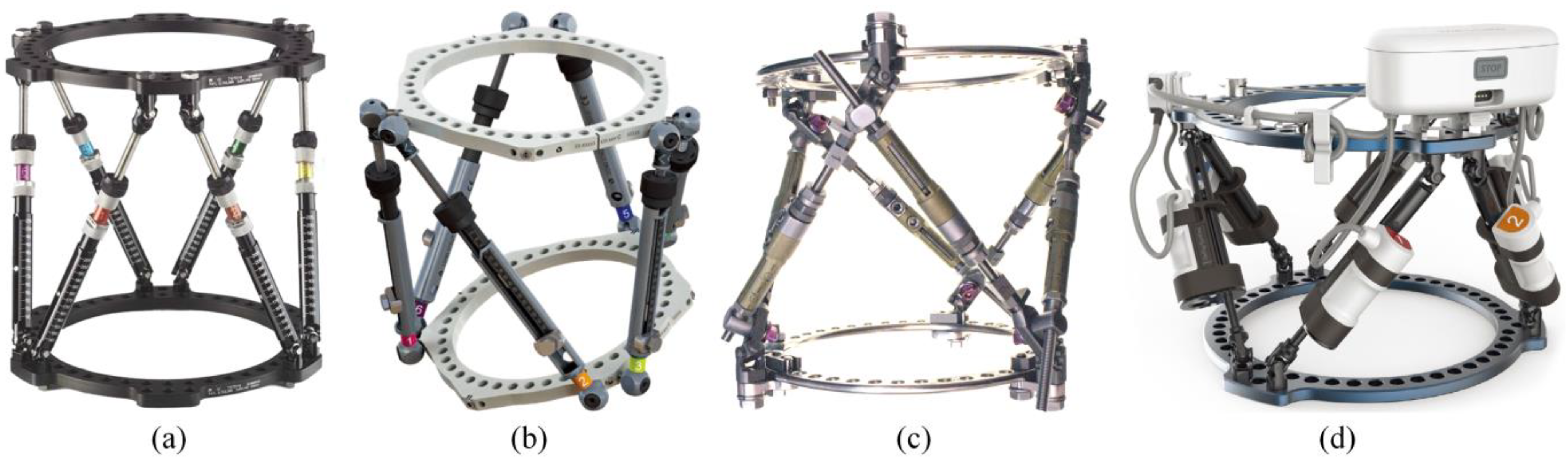
2. Descriptions of the Mechanism and Markers

Since each fixation ring connects rigidly to the bone segments, the relative movement of bone segments can be considered equal to that of the fixation rings under clinical precision. Therefore, the kinematic state of bones and rings can be uniformly described with the mechanism’s pose, avoiding measuring image parameters from the irregular geometry of bones. Image markers and their layout on the mechanism are also described.

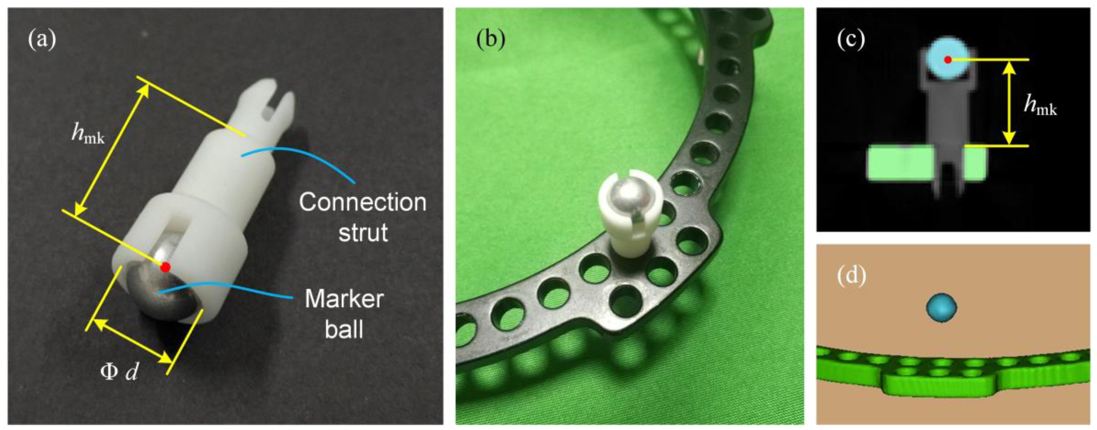
2.1. Image Marker Design

As shown in Figure 2, an image marker was designed to locate the 6-axis external fixation mechanism (denoted in the following as the 6-SPS mechanism, for convenience) in the CT image space. The image marker consists of a marker ball made of aluminum alloy, and a connection rod made of photosensitive resin. The connection rod is manufactured by rapid prototyping, and its bottom buckle is suitable for the connection holes of the fixation ring in various products. After the marker is installed, the structure of the connection rod ensures the distance between marker ball’s center and the installing plane of the fixation ring as $h_{\mathrm{mk}}$. Utilizing the difference of X-ray attenuation between the connecting rod and the marker ball, the region of the marker ball in the CT image can be segmented automatically using threshold division technology. Consequently, the 3D reconstruction model of the marker balls is obtained independently and without manual labor.

To identify the position vector $m$ of a marker ball in the CT image space, perform a 3D reconstruction of the marker ball and extract the surface point cloud data, then, fit the data into a sphere by a data fitting algorithm (for example, the least square method). The center of the sphere determines the position vector $m$.

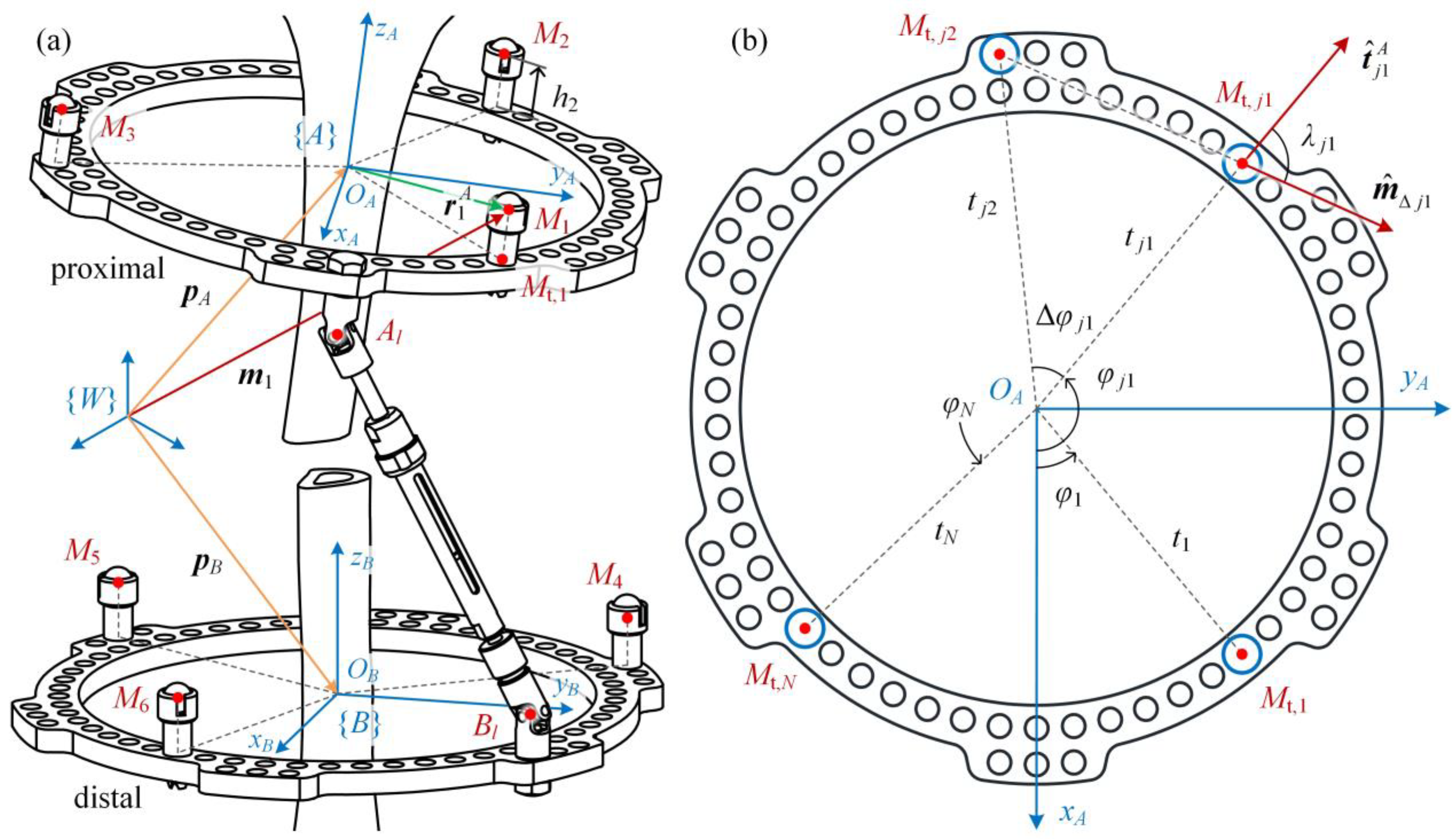
2.2. Pose Description of the Mechanism

The two fixation rings of a 6-SPS mechanism are clinically named the proximal ring and the distal ring, following anatomical direction. Install $N$ image markers on each ring for pose recognition; $2N$ markers are used in total. The $N$ markers on the same ring are inserted on the same side of the ring plane, and their placement is left to the surgeon’s choice. Because the identified marker position $m$ contains errors, the marker layout will impact the accuracy of the pose recognition, which will be discussed in Section 4.

Assume $2N=6$. Figure 3a illustrates the proximal ring, the distal ring, the support strut $l (l=1,2,\cdots ,6)$, the bone segments, and the image markers. The proximal ring, the distal ring, and the $l$th support strut are designated as the moving platform, the base platform, and the $l$th limb, respectively. Denote the reference frame of the image space as the image frame $\left\{W\right\}$. Establish a frame $\left\{A\right\}$ fixed to the moving platform with its origin $O_A$ at the center of the upper plane of the platform, $z_A$-axis perpendicular upward to the platform, $x_A$-axis toward the geometric front of the platform, and $y_A$-axis determined by the right-hand rule. Similarly, a frame $\left\{B\right\}$ is established for the base platform. The points $A_l$ and $B_l$ are the rotation centers of the two spherical joints on the $l$th limb, which connects to the moving platform and the base platform, respectively.

The pose of the 6-SPS mechanism is described by the relative pose of frame $\left\{A\right\}$ with respect to frame $\left\{B\right\}$, that is, the mechanism’s operational space pose. The poses of the moving platform and the base platform in the CT image space need to be determined first. Number the markers on the moving platform from 1 to $N$, beginning from the $x_A$-axis and increasing around the positive direction of $z_A$-axis. The markers on the base platform are numbered from $N+1$ to $2N$ similarly. The point $M_i$ is the center of the marker ball $i (i=1,2,\cdots ,2N)$, whose position vector is the marker position $m_i$ identified previously, and will be used to determine the pose $X_A={\left(\begin{array}{cc}{p}_A^{\mathrm{T}}& {\theta }_A^{\mathrm{T}}\end{array}\right)}^{\mathrm{T}}$ and $X_B={\left(\begin{array}{cc}{p}_B^{\mathrm{T}}& {\theta }_B^{\mathrm{T}}\end{array}\right)}^{\mathrm{T}}$ of frame $\left\{A\right\}$ and frame $\left\{B\right\}$, respectively. The position vectors $p_A$, $p_A$ and orientation vectors ${\theta }_A$, ${\theta }_B$ of pose $X_A$ and $X_B$ consist of parameters.

$$p_A={\left(\begin{array}{ccc}{x}_A& y_A& z_A\end{array}\right)}^{\mathrm{T}}, p_B={\left(\begin{array}{ccc}{x}_B& y_B& z_B\end{array}\right)}^{\mathrm{T}}, {\theta }_A={\left(\begin{array}{ccc}{\alpha }_A& {\beta }_A& {\gamma }_A\end{array}\right)}^{\mathrm{T}}, {\theta }_B={\left(\begin{array}{ccc}{\alpha }_B& {\beta }_B& {\gamma }_B\end{array}\right)}^{\mathrm{T}}$$

(1)

Wherein, orientation parameters $\alpha$, $\beta$ and $\gamma$ are the three sequential rotation angles of the X-Y-Z fixed angles rotation, which characterize the orientation of the frame $\left\{A\right\}$ or $\left\{B\right\}$ by the orientation matrix

$$R=\left[\begin{array}{ccc}\mathrm{c}\beta \mathrm{c}\gamma & \mathrm{s}\alpha \mathrm{s}\beta \mathrm{c}\gamma -\mathrm{c}\alpha \mathrm{s}\gamma & \mathrm{c}\alpha \mathrm{s}\beta \mathrm{c}\gamma +\mathrm{s}\alpha \mathrm{s}\gamma \\ \mathrm{c}\beta \mathrm{s}\gamma & \mathrm{s}\alpha \mathrm{s}\beta \mathrm{s}\gamma +\mathrm{c}\alpha \mathrm{c}\gamma & \mathrm{c}\alpha \mathrm{s}\beta \mathrm{s}\gamma -\mathrm{s}\alpha \mathrm{c}\gamma \\ -\mathrm{s}\beta & \mathrm{s}\alpha \mathrm{c}\beta & \mathrm{c}\alpha \mathrm{c}\beta \end{array}\right]$$

(2)

where $\mathrm{s}$ and $\mathrm{c}$ are the sine and cosine operators, respectively. According to the general body direction of patients in CT scans, each orientation parameter is within the range $(-90°,90°)$. Thus they can be determined by the entries $R_{21}$ at row 2 column 1, $R_{31}$ at row 3 column 1, and $R_{32}$ at row 3 column 2 of the orientation matrix $R$ as

$$\beta =-\arcsin R_{31}, \alpha =\arcsin (R_{32}/\cos \beta ), \gamma =\arcsin (R_{21}/\cos \beta )$$

(3)

Once the pose parameters of the two platforms are identified, the mechanism’s pose can be calculated as

$$p_{\mathrm{E}}=R_B^{-1}(p_A-p_B), R_{\mathrm{E}}=R_B^{-1}{R}_A$$

(4)

here $R_B^{-1}$ is the inverse matrix of the orientation matrix $R_B$. The position vector $p_{\mathrm{E}}={\left(\begin{array}{ccc}{x}_{\mathrm{E}}& y_{\mathrm{E}}& z_{\mathrm{E}}\end{array}\right)}^{\mathrm{T}}$ and orientation vector ${\theta }_{\mathrm{E}}={\left(\begin{array}{ccc}{\alpha }_{\mathrm{E}}& {\beta }_{\mathrm{E}}& {\gamma }_{\mathrm{E}}\end{array}\right)}^{\mathrm{T}}$ derived from $R_{\mathrm{E}}$ describe the pose of the mechanism’s operational space. Denote the pose of the 6-SPS mechanism as $X_{\mathrm{E}}={\left(\begin{array}{cc}{p}_{\mathrm{E}}^{\mathrm{T}}& {\theta }_{\mathrm{E}}^{\mathrm{T}}\end{array}\right)}^{\mathrm{T}}$, establishing a pose description of the mechanism.

2.3. Layout Description of Markers

Using the identified position $m_i$ of an image marker, one point $M_i$ on the mechanism can be located in the CT image space. In order to recognize the pose of the mechanism, the layout information of the markers is required. The marker layout is parametrically described here, including the marker’s number $N$, and the installation parameters $t_i$, ${\phi }_i$ and $h_i$ of each marker $i$.

Take the marker layout on frame $\left\{A\right\}$ as an illustration. As shown in Figure 3, denote the projection of point $M_i$ onto the $x_A{y}_A$-plane as point $M_{t,i}$, the distance between points $O_A$ and $M_{\mathrm{t},i}$ as radius $t_i$, the rotation angle from the $x_A$-axis to the vector $\overrightarrow{O_A{M}_{t,i}}$ around the $z_A$-axis as sweep angle ${\phi }_i$, and the signed distance from the $x_A{y}_A$-plane to point $M_i$ as height $h_i$. The height $h_i$ is determined by the marker’s dimension $h_{\mathrm{mk}}$ and the platform’s thickness $h_{\mathrm{plt}}$, that $h_i=h_{\mathrm{mk}}$ for the marker installed on the plane or $h_i=-h_{\mathrm{mk}}-h_{\mathrm{plt}}$ for beneath the plane. The difference between sweep angles ${\phi }_{i+1}$ and ${\phi }_i$ is defined as the included angle $\Delta {\phi }_i={\phi }_{i+1}-{\phi }_i$. Using the installation parameters, the position vector of point $M_i$ can be expressed as

$$r_i^A={\left(\begin{array}{ccc}{t}_i\cos {\phi }_i& t_i\sin {\phi }_i& h_i\end{array}\right)}^{\mathrm{T}}$$

(5)

which describes the layout of each marker.

3. Pose Recognition of the Mechanism

This section proposes a pose recognition method by identifying the position and orientation parameters of the 6-SPS mechanism. Based on the marker layout parameters, this recognition method adopts an analytical approach to solving the issue of numerical solutions. The pose recognition of each platform is presented by taking frame $\left\{A\right\}$ as an example, and then the pose of the mechanism’s operational space is determined.

3.1. Establishing Position Relationships of Markers

Based on the vector chain formed by the origin $O_A$ and position vector $r_i^A$ in image frame $\left\{W\right\}$ (Figure 3a), the closed-loop vector equation regarding the marker $i$ is

$$p_A+R_A{r}_i^A-m_i=0$$

(6)

If $N=2$ markers are used, two points on the platform are settled, with one rotational freedom around the axis passing through these points. In other words, the solution of Equation (6), which includes two vector equations, is uncertain. Therefore, a minimum of three markers should be used for the pose recognition of a frame. Using $N\ge 3$ markers, the pose $X_A$ of frame $\left\{A\right\}$ can be identified by solving Equation (6). In order to implement analytical solutions, marker groups and geometric conditions are utilized.

3.2. Setting Up Marker Groups

Set up $N$ groups of markers, such that three markers $j_1=j$, $j_2=j+\mathrm{floor}(N/3)$, and $j_3=j+\mathrm{floor}(2N/3)$ are included in the group $j (j=1,2,\cdots ,N)$. Herein, $\mathrm{floor}(\cdot )$ is the round-down function, and the addition computation of the marker numbers $j_2$ and $j_3$ follows an N-based overflow. Taking $N=6$ markers as an example, the group $j=3$ includes markers numbered $j_1=3$, $j_2=5$ and $j_3=1$. Determine the install parameters $t_{j1}$, ${\phi }_{j1}$, …, $r_{j3}$. Each group can be used to identify one set of pose parameters.

3.3. Identifying Pose Parameters of Each Group

Consider the parameter identification of group $j$. Denote the unit vectors of $x_A$-axis and $z_A$-axis as ${\widehat{u}}_{A(j)}$ and ${\widehat{w}}_{A(j)}$, respectively. The unit vector ${\widehat{v}}_{A(j)}$ of $y_A$-axis and the orientation matrix $R_{A(j)}$ of frame $\left\{A\right\}$ satisfy

$$R_{A(j)}=\left[\begin{array}{ccc}{\widehat{u}}_{A(j)}& {\widehat{v}}_{A(j)}& {\widehat{w}}_{A(j)}\end{array}\right]=\left[\begin{array}{ccc}{\widehat{u}}_{A(j)}& {\widehat{w}}_{A(j)}\times {\widehat{u}}_{A(j)}& {\widehat{w}}_{A(j)}\end{array}\right]$$

(7)

Based on the identified positions $m_{j1}$, $m_{j2}$ and $m_{j3}$ of marker $j_1$, $j_2$ and $j_3$, use their relative positions

$$m_{\Delta j1}=m_{j1}-m_{j2}, m_{\Delta j2}=m_{j2}-m_{j3}$$

(8)

to determine the unit vector of $z_A$-axis as

$${\widehat{w}}_{A(j)}=(m_{\Delta j1}\times m_{\Delta j2})/\Vert m_{\Delta j1}\times m_{\Delta j2}\Vert$$

(9)

where $\Vert \cdot \Vert$ represents the 2-norm of a vector. Taking the frame $\left\{A\right\}$ as a reference, the position vector $t_{j1}^A$ of the projection point $M_{\mathrm{t},j1}$ is invariant, and its unitization yields

$${\widehat{t}}_{j1}^A={\left(\begin{array}{ccc}\cos {\phi }_{j1}& \sin {\phi }_{j1}& 0\end{array}\right)}^{\mathrm{T}}$$

(10)

In the image frame $\left\{W\right\}$, the description of vector ${\widehat{t}}_{j1}^A$ becomes $R_A{\widehat{t}}_{j1}^A$. The unitized relative position vector

$${\widehat{m}}_{\Delta j1}=m_{\Delta j1}/\Vert m_{\Delta j1}\Vert$$

(11)

and vector $R_A{\widehat{t}}_{j1}^A$ satisfy an axis-angle rotation relationship (Figure 3b): the vector $R_A{\widehat{t}}_{j1}^A$ is the result of vector ${\widehat{m}}_{\Delta j1}$ rotating in the positive direction about $z_A$-axis at angle ${\lambda }_{j1}$. Expressing the axis-angle rotation with a transformation matrix $R_{{\widehat{w}}_{A(j)},{\lambda }_{j1}}$ yields

$$R_A{\widehat{t}}_{j1}^A=R_{{\widehat{w}}_{A(j)},{\lambda }_{j1}}{\widehat{m}}_{\Delta j1}$$

(12)

Utilizing the Rodrigues formula, it is feasible to calculate the transformation matrix as

$$R_{{\widehat{w}}_{A(j)},{\lambda }_{j1}}=I+\left[{\widehat{w}}_{A(j)}\times \right]\sin {\lambda }_{j1}+{\left[{\widehat{w}}_{A(j)}\times \right]}^2(1-\cos {\lambda }_{j1})$$

(13)

where $I$ represents $3\times 3$ identity matrix, and $\left[{\widehat{w}}_{A(j)}\times \right]$ is the skew-symmetric matrix of vector ${\widehat{w}}_{A(j)}$. The angle ${\lambda }_{j1}$ of the axis-angle rotation can be calculated with the included angle $\Delta {\phi }_{j1}={\phi }_{j2}-{\phi }_{j1}$ as

$${\lambda }_{j1}=\arcsin \left((t_{j2}/\Vert \overrightarrow{M_{t,j1}{M}_{t,j2}}\Vert )\sin \Delta {\phi }_{j1}\right), \Vert \overrightarrow{M_{t,j1}{M}_{t,j2}}\Vert =\sqrt{t_{j1}^2+t_{j2}^2-2t_{j1}{t}_{j2}\cos \Delta {\phi }_{j1}}$$

(14)

Substituting Equations (7) and (10) into Equation (12) leads to a linear equation system about the vector ${\widehat{u}}_{A(j)}$:

$$(I\cos {\phi }_{j1}+\left[{\widehat{w}}_{A(j)}\times \right]){\widehat{u}}_{A(j)}=R_{{\widehat{w}}_{A(j)},{\lambda }_{j1}}{\widehat{m}}_{\Delta j1}$$

(15)

Denote the coefficient matrix of Equation (15) as $G_{A(j)}$. If $\cos {\phi }_{j1}\ne 0$, the inverse matrix $G_{A(j)}^{-1}$ of coefficient matrix $G_{A(j)}$ exists, and the solution of ${\widehat{u}}_{A(j)}$ is

$${\widehat{u}}_{A(j)}=G_{A(j)}^{-1}{R}_{{\widehat{w}}_{A(j)},{\lambda }_{j1}}{\widehat{m}}_{\Delta j1}$$

(16)

Elseif $\cos {\phi }_{j1}=0$, the vector ${\widehat{t}}_{j1}^A$ becomes ${\left(\begin{array}{ccc}0& 1& 0\end{array}\right)}^{\mathrm{T}}$, and Equation (12) turns into

$${\widehat{v}}_{A\left(j\right)}=R_{{\widehat{w}}_{A\left(j\right)},{\lambda }_{j1}}{\widehat{m}}_{\mathsf{\Delta }j1}.$$

(17)

Now the rest vector ${\widehat{v}}_{A(j)}$ or ${\widehat{u}}_{A(j)}$ can be calculated by the right-hand rule, using the vectors ${\widehat{u}}_{A(j)}$ (from Equation (16)) and ${\widehat{w}}_{A(j)}$, or using ${\widehat{v}}_{A(j)}$ (from Equation (17)) and ${\widehat{w}}_{A(j)}$. Determine the matrix $R_{A(j)}$ by Equation (7) with vectors ${\widehat{u}}_{A(j)}$, ${\widehat{v}}_{A(j)}$ and ${\widehat{w}}_{A(j)}$, identify the orientation parameters ${\theta }_{A(j)}={\left(\begin{array}{ccc}{\alpha }_{A(j)}& {\beta }_{A(j)}& {\gamma }_{A(j)}\end{array}\right)}^{\mathrm{T}}$ of group $j$.

For identification of the position parameters, substituting the previously obtained orientation matrix $R_{A(j)}$, the identified position $m_{j1}$ and the installation position $r_{j1}^A$ of marker $j_1$ into Equation (6) leads to

$$p_{A(j)}={\left(\begin{array}{ccc}{x}_{A(j)}& y_{A(j)}& z_{A(j)}\end{array}\right)}^{\mathrm{T}}=m_{j1}-R_{A(j)}{r}_{j1}^A$$

(18)

3.4. Recognizing the Mechanism’s Pose

The above step has identified $N$ groups of position and orientation parameters. Take the mean value of the identified position parameter $p_{A(j)}$ and orientation parameter ${\theta }_{A(j)}$ to determine the recognized pose of frame $\left\{A\right\}$:

$$X_A={\left(\begin{array}{cc}{p}_A^{\mathrm{T}}& {\theta }_A^{\mathrm{T}}\end{array}\right)}^{\mathrm{T}}=\frac{1}{N}{\displaystyle \sum _{j=1}^N{\left(\begin{array}{cc}{p}_{A(j)}^{\mathrm{T}}& {\theta }_{A(j)}^{\mathrm{T}}\end{array}\right)}^{\mathrm{T}}}$$

(19)

For the pose $X_B$ of frame $\left\{B\right\}$, utilize the markers $i=N+1,N+2,\cdots 2N$ on the base platform and identify the position and orientation parameters similarly. After identifying the pose of moving platform $X_A$ and that of base platform $X_B$ in the image space, finish the pose recognition of the mechanism’s operational space $X_E$ by Equation (4).

4. Marker Layout Principles

The main error factors affecting the accuracy of pose recognition using image markers are CT scanning resolution limit, reconstruction point cloud distortion, image marker dimension error, and installation position error. In the clinical environment, it is difficult to reduce these error factors directly. This section establishes an error mapping model between the error factors and the pose recognition errors, and discusses the appropriate range of the marker layout.

4.1. Error Modeling of the Pose Recognition

The error model is about the pose recognition of a frame ($\left\{A\right\}$ or $\left\{B\right\}$), and the subscript is omitted for simplicity. For the $N$ markers utilized by the pose recognition of a frame, use image error parameters $\Delta m_i={\left(\begin{array}{ccc}\delta x_{m,i}& \delta y_{m,i}& \delta z_{m,i}\end{array}\right)}^{\mathrm{T}}$ to represent the systematic error of CT scan and 3D reconstruction, and installation error parameters $\Delta {\eta }_i={\left(\begin{array}{ccc}\delta t_i& \delta {\phi }_i& \delta h_i\end{array}\right)}^{\mathrm{T}}$ to represent the dimensional error of the marker’s manufacture and installation. These error parameters are relatively small compared to the structural dimensions and installation parameters of the markers. Therefore, the linear approach is used to establish the differential error model of pose recognition. Denote the $6N$ error parameters as a vector

$${\left(\begin{array}{cc}\Delta m^{\mathrm{T}}& \Delta {\eta }^{\mathrm{T}}\end{array}\right)}^{\mathrm{T}}={\left(\begin{array}{cccccc}\Delta m_1^{\mathrm{T}}& \cdots & \Delta m_N^{\mathrm{T}}& \Delta {\eta }_1^{\mathrm{T}}& \cdots & \Delta {\eta }_N^{\mathrm{T}}\end{array}\right)}^{\mathrm{T}}$$

(20)

With regard to the identified pose parameters $X={\left(\begin{array}{cc}{p}^{\mathrm{T}}& {\theta }^{\mathrm{T}}\end{array}\right)}^{\mathrm{T}}$, calculating Jacobian matrix produces the error mapping model between the error parameters ${\left(\begin{array}{cc}\Delta m^{\mathrm{T}}& \Delta {\eta }^{\mathrm{T}}\end{array}\right)}^{\mathrm{T}}$ and the pose recognition errors $\Delta X={\left(\begin{array}{cc}\Delta p^{\mathrm{T}}& \Delta {\theta }^{\mathrm{T}}\end{array}\right)}^{\mathrm{T}}$:

$$\Delta X=\left[\begin{array}{cccccc}\frac{\partial p}{\partial m_1}& \cdots & \frac{\partial p}{\partial m_N}& \frac{\partial p}{\partial {\eta }_1}& \cdots & \frac{\partial p}{\partial {\eta }_N}\\ \frac{\partial \theta }{\partial m_1}& \cdots & \frac{\partial \theta }{\partial m_N}& \frac{\partial \theta }{\partial {\eta }_1}& \cdots & \frac{\partial \theta }{\partial {\eta }_N}\end{array}\right]\left(\begin{array}{c}\Delta m_1\\ ⋮\\ \Delta m_N\\ \Delta {\eta }_1\\ ⋮\\ \Delta {\eta }_N\end{array}\right)=J\left(\begin{array}{c}\Delta m\\ \Delta \eta \end{array}\right)$$

(21)

Each submatrix of Jacobian matrix $J$ in Equation (21) represents the derivative matrix of the corresponding identified pose parameters with respect to error parameters, for instance,

$$\frac{\partial p}{\partial m_1}=\left[\begin{array}{ccc}\frac{\partial x}{\partial x_{m,1}}& \frac{\partial x}{\partial y_{m,1}}& \frac{\partial x}{\partial z_{m,1}}\\ \frac{\partial y}{\partial x_{m,1}}& \frac{\partial y}{\partial y_{m,1}}& \frac{\partial y}{\partial z_{m,1}}\\ \frac{\partial z}{\partial x_{m,1}}& \frac{\partial z}{\partial y_{m,1}}& \frac{\partial z}{\partial z_{m,1}}\end{array}\right], \frac{\partial \theta }{\partial {\eta }_N}=\left[\begin{array}{ccc}\frac{\partial \alpha }{\partial t_N}& \frac{\partial \alpha }{\partial {\phi }_N}& \frac{\partial \alpha }{\partial h_N}\\ \frac{\partial \beta }{\partial t_N}& \frac{\partial \beta }{\partial {\phi }_N}& \frac{\partial \beta }{\partial h_N}\\ \frac{\partial \gamma }{\partial t_N}& \frac{\partial \gamma }{\partial {\phi }_N}& \frac{\partial \gamma }{\partial h_N}\end{array}\right]$$

(22)

4.2. Analyzing the Effect of Marker Layout Variations

By considering the Jacobian matrix $J$ as a function of the marker’s number and installation parameters, the trend of pose recognition errors versus the variation of marker layout can be found. According to the Monte Carlo method, assume that the error parameters conform to a certain probability distribution, and consider the pose recognition as a random sampling. Hence, the accuracy of pose recognition using a particular marker layout can be expressed as a mathematical expectation, which is derived from the recognition errors of multiple sampling.

Based on the error sensitivity analysis method [28,29], the Jacobian matrix $J$ suggests that the installation parameter variations of radius $t_i$ and height $h_i$ have little effect on the error mapping. Therefore, the effect of the marker’s number $N$ and sweep angle ${\phi }_i$ is investigated here. A single-factor analysis approach is developed for the effect of marker layout variations. Based on computer simulation, the approach includes the following steps (Figure 4):

(1)

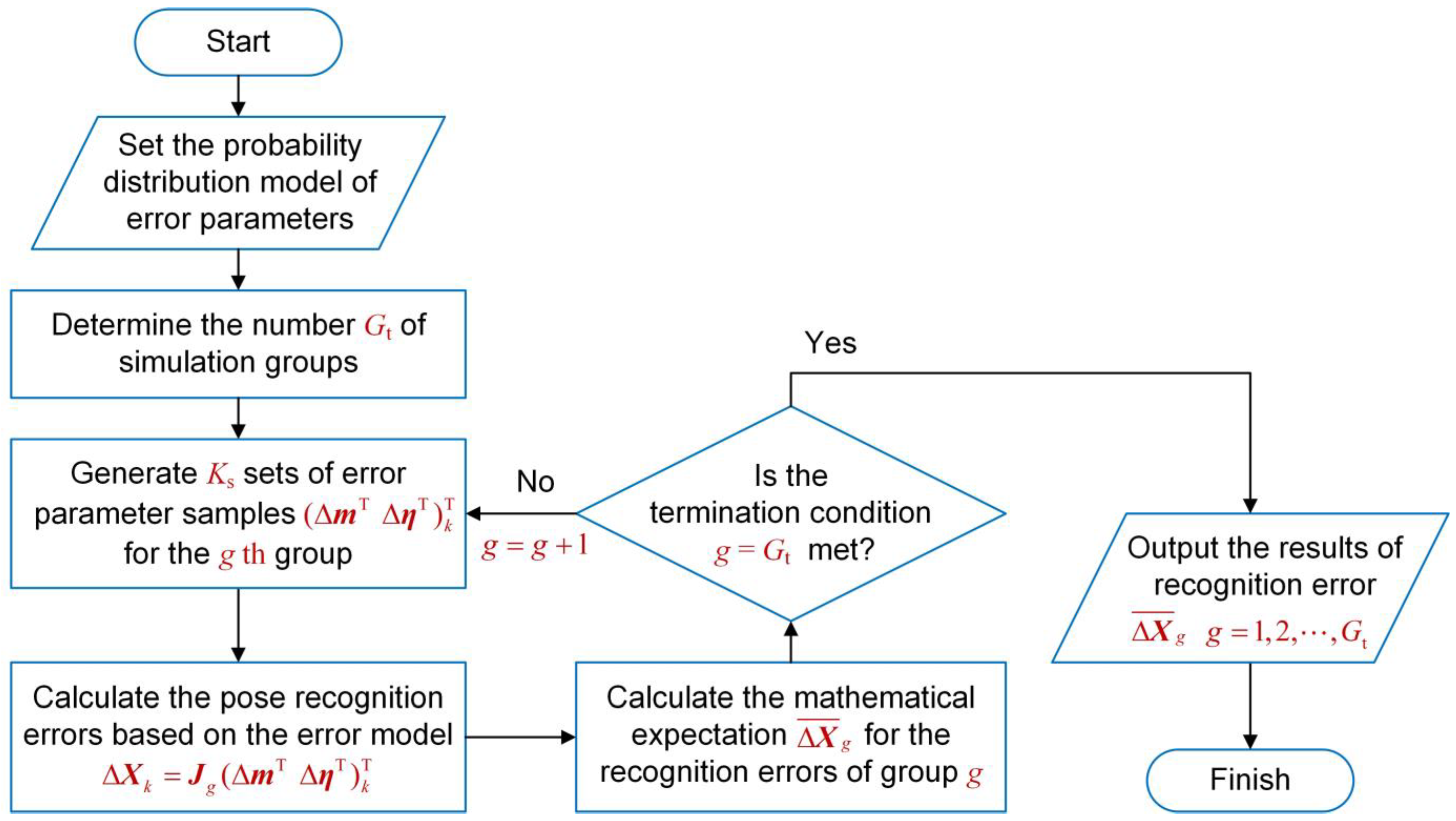
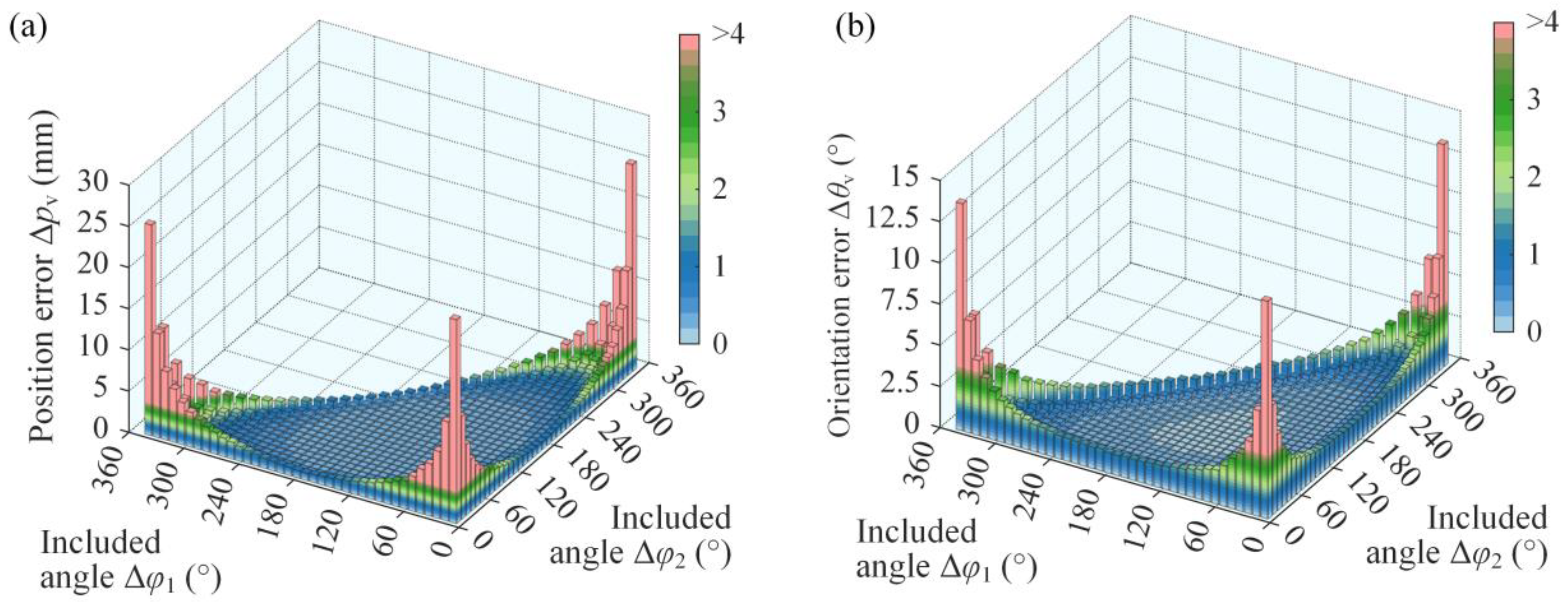
Configure the probability distribution to generate error parameters for each random sampling. A total of $G_{\mathrm{t}}$ simulation groups were set univariately about the marker’s number $N$ and sweep angle ${\phi }_i$. For the groups regarding the variation of number, take $N=3,4,5,\cdots$. For the groups regarding the variation of sweep angle, adopt combinations of discrete angles ${\phi }_i=\psi ,2\psi ,3\psi ,\cdots$ based on an interval $\psi$, and ensure that all included angles satisfy the condition $\Delta {\phi }_1+\Delta {\phi }_2+\cdots +\Delta {\phi }_N=360°$.

(2)

Generate $K_{\mathrm{s}}$ samples of random error parameters ${(\begin{array}{cc}\Delta m^{\mathrm{T}}& \Delta {\eta }^{\mathrm{T}}\end{array})}_k^{\mathrm{T}}$ for the simulation group $g (g=1,2,\cdots ,G_{\mathrm{t}})$, and calculate the Jacobian matrix $J_g$ for the particular marker layout of this group (given parameters $N$, $t_i$, ${\phi }_i$ and $h_i$). The corresponding pose recognition errors of $K_{\mathrm{s}}$ samples are

$$\Delta X_k=J_g{\left(\begin{array}{cc}\Delta m^{\mathrm{T}}& \Delta {\eta }^{\mathrm{T}}\end{array}\right)}_k^{\mathrm{T}} (k=1,2,\cdots ,K_{\mathrm{s}})$$

(23)

(1)

Take the absolute value of each sample, and calculate their expectation as

$${\overline{\Delta X}}_g=\frac{1}{K_{\mathrm{s}}}{\displaystyle \sum _{k=1}^{K_{\mathrm{s}}}\left|\Delta X_k\right|}$$

(24)

The expectation ${\overline{\Delta X}}_g$ represents the pose recognition accuracy about the marker layout adopted by group $g$.

(4)

Repeat steps 2–3 to assess the pose recognition accuracy of all simulation groups. Analyze the trend of pose recognition accuracy versus the variation of layout parameters, and further determine the marker layout principles.

4.3. Determining the Marker Layout Principles

According to our previous tests and relevant literature [30,31,32], assume that the image error parameters $\delta x_{m,i}$, $\delta y_{m,i}$ and $\delta z_{m,i}$ follow a normal distribution of $\mathrm{N}\left(0,{0.3}^2\right)$. Take the marker’s installation deviations as position errors along the three principal axes of frame $\left\{A\right\}$ or $\left\{B\right\}$. Regarding the manufacturing tolerance, the distribution of installation deviations is determined as ${\epsilon }_{x,i},{\epsilon }_{y,i},{\epsilon }_{z,i}\sim \mathrm{N}\left(0,{(0.4/6)}^2\right)$ based on the three-sigma rule. Then, the installation error parameters are calculated as

$$\{\begin{array}{l}\delta t_i={\epsilon }_{x,i}\cos {\phi }_i+{\epsilon }_{y,i}\sin {\phi }_i\\ \delta {\phi }_i=(-{\epsilon }_{x,i}\sin {\phi }_i+{\epsilon }_{y,i}\cos {\phi }_i)\cdot (180°/\pi t_i)\\ \delta h_i={\epsilon }_{z,i}\end{array}$$

(25)

4.3.1. The Number Principle

The simulation groups about the marker’s number take $N=3,4,\cdots ,10$. The installation radius $t_i=100\mathrm{mm}$ and height $h_i=20\mathrm{mm}$ are fixed, and the sweep angle ${\phi }_i$ is set following the markers evenly distributed along the platform’s circumferential direction. For each simulation group, $K_{\mathrm{s}}=2000$ samples are generated, and the accuracy of pose recognition is evaluated. The results are shown in Figure 5.

In the same group, the recognition error of position parameter $z$ and orientation parameter $\gamma$ are slightly smaller than those of other position and orientation parameters. This agrees with the findings of the error sensitivity analysis, in that the sensitivity coefficients mapping error parameters ${(\begin{array}{cc}\Delta m^{\mathrm{T}}& \Delta {\eta }^{\mathrm{T}}\end{array})}_k^{\mathrm{T}}$ to pose recognition errors $\Delta z$ and $\Delta \gamma$ are relatively low. Among the different groups, increasing the number of markers reduces the recognition errors partly, but not by order of magnitude. The pose recognition errors using $N=3$ markers are

$${\overline{\Delta X}}_{(3\mathrm{mks})}={\left(\begin{array}{cccccc}0.165\mathrm{mm}& 0.164\mathrm{mm}& 0.137\mathrm{mm}& 0.103°& 0.106°& 0.079°\end{array}\right)}^{\mathrm{T}}$$

(26)

while increasing the marker number to $N=6$ reduces the pose recognition errors by 27% in position and 25% in orientation. Considering the practicability and accuracy comprehensively, establish the principle of marker number as $N=3$.

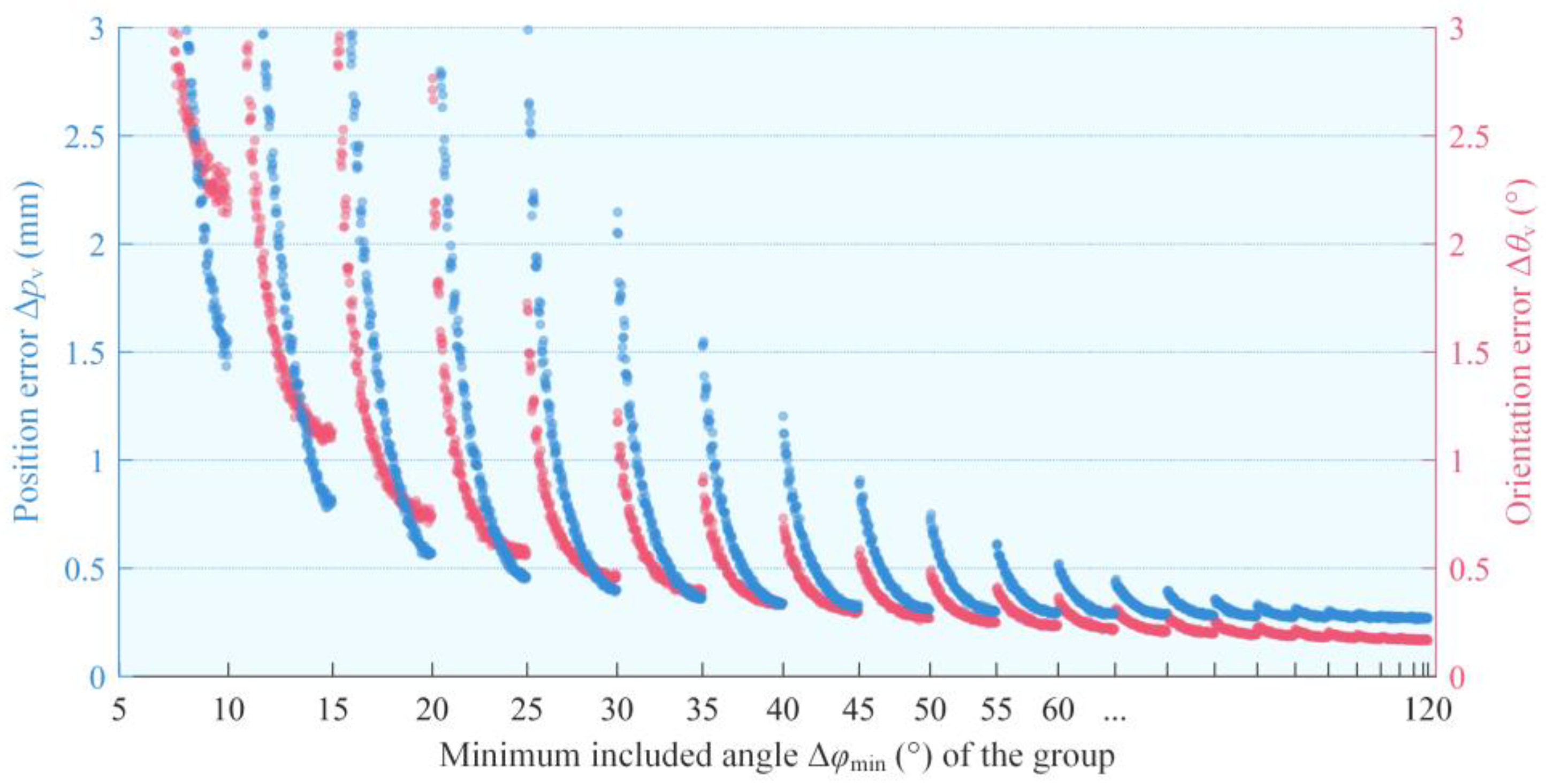
4.3.2. The Sweep Angle Principle

Based on the preceding established number principle $N=3$, the different combinations of sweep angles ${\phi }_i (i=1,2,3)$ are taken for the simulation groups about the marker’s sweep angle. The remaining installation parameters are $t_i=100\mathrm{mm}$ and $h_i=20\mathrm{mm}$. According to the rotational symmetry of the platform, the first marker can be placed at the $x$-axis of the platform, that is ${\phi }_1=0$. The sweep angles ${\phi }_2$ and ${\phi }_3$ are discretized with an interval $\psi =5°$ in a possible range, making the included angles satisfying

$$\Delta {\phi }_1+\Delta {\phi }_2+\Delta {\phi }_3=360°$$

(27)

The accuracy of each group’s pose recognition was then evaluated by taking $K_{\mathrm{s}}=2000$ samples. For clarity, the pose recognition accuracy was expressed as volume errors of position $\Delta p_{\mathrm{v}}$ and orientation $\Delta {\theta }_{\mathrm{v}}$, and the results are shown in Figure 6.

$$\Delta p_{\mathrm{v}}=\sqrt{\Delta x^2+\Delta y^2+\Delta z^2}, \Delta {\theta }_{\mathrm{v}}=\sqrt{\Delta {\alpha }^2+\Delta {\beta }^2+\Delta {\gamma }^2}$$

(28)

The pose recognition errors decrease with the values of included angles $\Delta {\phi }_1$ and $\Delta {\phi }_2$ converging and their sum $\Delta {\phi }_1+\Delta {\phi }_2$ approaching 240°, showing that evenly distributing markers on a platform reduces recognition errors. To determine the principle of the marker’s sweep angle, the included angles $\Delta {\phi }_1$, $\Delta {\phi }_2$ and $\Delta {\phi }_3$ of each simulation group were arranged ascendingly intra-group, and then the groups were sorted according to the minimum-median-maximum priority of the included angle (Figure 7).

The scatters between two adjacent scales on the horizontal axis of Figure 7 are the groups whose minimum included angle equals the smaller scale value. The scatters from left to right represent the groups sorted with the minimum-median-maximum priority. Accoridng to the vertical axis value of the scatters, when the minimum and median included angles were both greater than 45°, the position and orientation recognition errors were less than 0.9 mm and 0.6°. If the minimum included angle reaches 15°, a difference between the maximum and median included angles of less than 150° and permitted recognition errors of less than 1 mm and 0.8°.

Based on the preceding analysis, the following are the layout principles for markers: use $N=3$ markers for each platform, the minimum included angle $\Delta {\phi }_{\min }\ge 45°$ and median included angle $\Delta {\phi }_{\mathrm{med}}\ge 45°$; for limited installation conditions, $\Delta {\phi }_{\min }\ge 15°$ and the difference between maximum and median included angles $\Delta {\phi }_{\max }-\Delta {\phi }_{\mathrm{med}}\le 150°$.

5. Error Compensation Strategy and Experiments

By installing markers following the proposed marker layout principles, the pose recognition errors can be kept within a small range. Compensating the recognized pose errors can further improve the accuracy of the correction results. Although current clinical practice lacks instruments for directly measuring pose errors, the commercial fixators ensure a certain degree of precision in the dimensions of their structure. In addition, kinematic calibrations can be performed on external fixation robots to reduce positioning errors to 0.05% of their operational space’s scale [33,34]. Therefore, recognition errors can be compensated using the dimension parameters of the 6-SPS mechanism. Model experiments of fracture reduction are also carried out in this section.

5.1. Compensation for Pose Recognition Errors

The error compensation strategy implements compensation in the mechanism’s operational space. Denote the mechanism’s recognized pose as $X_{\mathrm{r}}$. Within the precision of clinical practice, the mechanism’s theoretical pose $X_{\mathrm{t}}$ can be considered equivalent to the mechanism’s actual pose and be used for compensation. $X_{\mathrm{t}}$ is calculated through the forward kinematics model of the mechanism with nominal dimensions and limb lengths. The nominal dimensions are replaced with their identified values if the mechanism has been calibrated. Referring to Figure 3a, utilize the points $A_l$ and $B_l$ to establish the closed-loop vector equation of limb $l$:

$$p_{\mathrm{t}}+R_{\mathrm{t}}{a}_l^A-b_l^B-q_{\mathrm{t},l}{\widehat{s}}_{\mathrm{t},l}=0(l=1,2,\cdots ,6)$$

(29)

where $p_{\mathrm{t}}$ and $R_{\mathrm{t}}$ are the position vector and orientation matrix corresponding to the theoretical pose $X_{\mathrm{t}}$, which are to be solved. $a_l^A$ and $b_l^B$ are the position vectors of point $A_l$ in frame $\left\{A\right\}$ and point $B_l$ in frame $\left\{B\right\}$, respectively, which are determined by the mechanism’s dimensions. $q_{\mathrm{t},l}{\widehat{s}}_{\mathrm{t},l}$ is the product of length $q_{\mathrm{t},l}$ and unit axis vector ${\widehat{s}}_{\mathrm{t},l}$ of the limb $l$. The limb length $q_{\mathrm{t},l}$ can be determined from the actual position of prismatic joint P (for example, the reading from motor encoders), while the vector ${\widehat{s}}_{\mathrm{t},l}$ can be eliminated by taking norm of Equation (29). Writing the normed equations in a functional form we have

$$f_l(X_{\mathrm{t}})=\Vert p_{\mathrm{t}}+R_{\mathrm{t}}{a}_l^A-b_l^B\Vert -q_{\mathrm{t},l}=0$$

(30)

Combine Equation (30) from limb 1 to limb 6 to establish the mechanism’s forward kinematics model, and the solution $X_{\mathrm{t}}$ can be obtained through numerical methods.

The recognition errors are calculated by the theoretical pose $X_{\mathrm{t}}$ as

$$\Delta X_{\mathrm{r}}=X_{\mathrm{r}}-X_{\mathrm{t}}$$

(31)

For the target pose $X_{\mathrm{a}}(t)$ at time $t$ of the planned trajectory, use the recognition errors $\Delta X_{\mathrm{r}}$ to determine the compensated pose $X_{\mathrm{c}}(t)$ as

$$X_{\mathrm{c}}(t)=X_{\mathrm{a}}(t)-\Delta X_{\mathrm{r}}$$

(32)

The compensated pose $X_{\mathrm{c}}(t)$ is finally applied for the mechanism to achieve deformity correction. Regarding the execution of the mechanism, establish the inverse kinematics model based on Equation (30) to determine the corresponding joint space trajectory:

$$q_{\mathrm{c},l}(t)=\Vert p_{\mathrm{c}}(t)+R_{\mathrm{c}}(t)a_l^A-b_l^B\Vert$$

(33)

where the position vector $p_{\mathrm{c}}(t)$ and orientation matrix $R_{\mathrm{c}}(t)$ are derived from the compensated pose $X_{\mathrm{c}}(t)$.

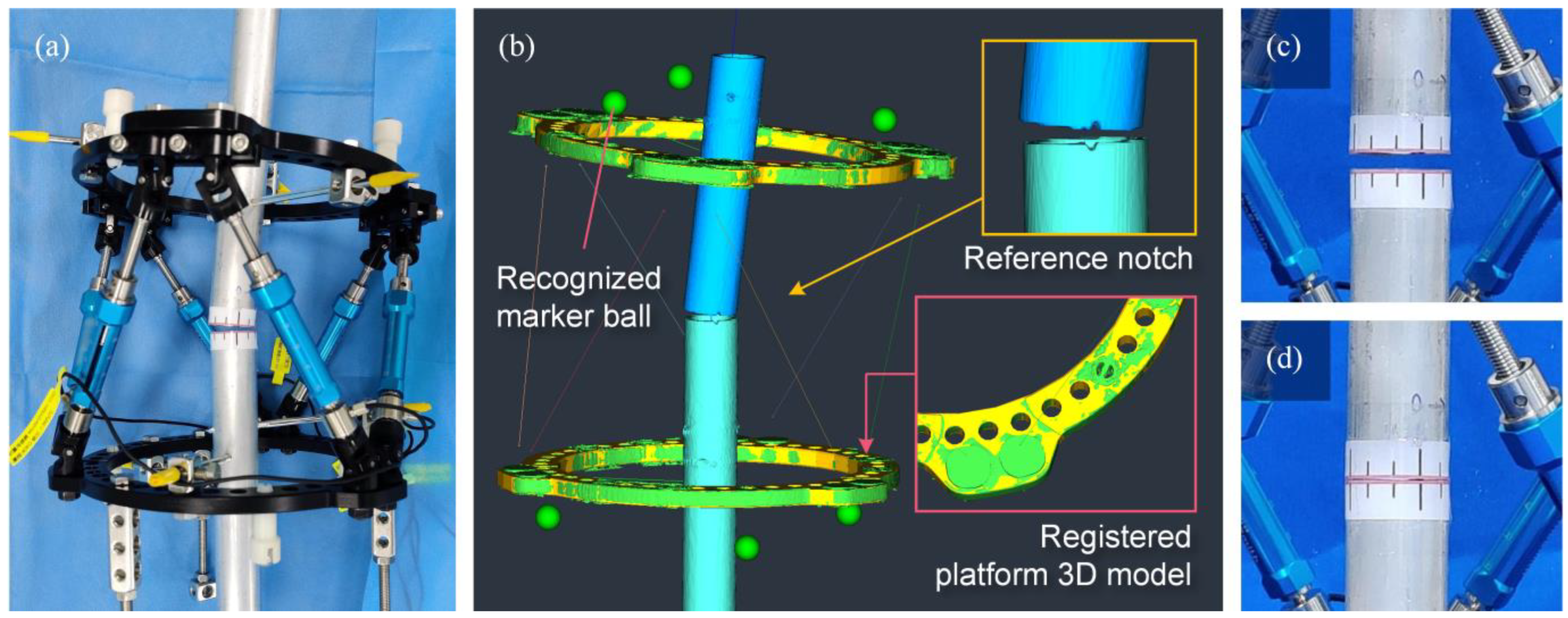
5.2. Model Experiments of Fracture Reduction

To evaluate the methods proposed, we conducted model experiments of fracture reduction, as shown in Figure 8. The experiments used a self-developed external fixation mechanism. Two aluminum cylinders simulated a fracture’s proximal and distal bone segments. Each adjacent end of the cylinders featured a notch and a circumferential scale for correction planning and accuracy assessment. The fracture model with the mechanism was assembled, and the experiments were carried out as follows. The complete procedure of the experiment is presented in the Supplementary Video Material.

(1)

Adjust the lengths of limbs 1–6 arbitrarily to construct a random pose of the mechanism, simulating the initial fracture state. Theoretical pose $X_{\mathrm{t}}$ is calculated according to the strut lengths $q_{\mathrm{t},l}$ provided by the motor encoders. Meanwhile, the relative initial pose $X_{\mathrm{md}0}$ of the cylinders is determined by measuring the point pairs from circumferential scales.

(2)

Install the markers following the proposed marker layout principles, and then perform a CT scan and 3D reconstruction of the entire model. The 3D model of the marker balls was obtained by automatic segmentation based on the feature of markers described in Section 2. The 3D models of cylinders and mechanism platforms were used for correction planning in visual, thus they could be obtained easily through approximate manual segmentation. The positions $m_i$ of markers were then identified, and the mechanism’s recognized pose $X_{\mathrm{r}}$ was determined by the proposed pose recognition method. Subsequently, the accuracy of pose recognition was analyzed by calculating the recognition errors $\Delta X_{\mathrm{r}}$. In addition, a visual inspection was performed by registering standard 3D models to the reconstruction models of the platforms, using the recognized poses of frames $\left\{A\right\}$ and $\left\{B\right\}$.

(3)

Using self-developed software, the 3D models of bone segments undergoing reduction motion were manipulated to design the fracture correction plan. The notch on the cylinder served as a reference point for the correction target. The correction motion was determined and the trajectory with target pose $X_{\mathrm{a}}(t)$ was generated. After error compensation, the mechanism executed the compensated trajectory $X_{\mathrm{c}}(t)$ and reduced the fracture model. The effectiveness of fracture reduction was evaluated by measuring the relative final pose $X_{\mathrm{md}1}$ of the cylinders.

A caliper with 0.02 mm resolution was utilized for measuring. A uCT760 instrument (United Imaging, Shanghai, China) and MIMICS 20.0 software (Materialise, Leuven, Belgium) were utilized for CT scan and 3D reconstruction. Pose recognition, trajectory planning, and motion control were accomplished in self-developed software. The mechanism has been calibrated to an accuracy of 0.0574 mm and 0.0294°.

Ten reduction experiments on the fracture model have been conducted. The statistical results of pose recognition errors $\Delta X_{\mathrm{r}}$ are shown in

Table 1. Pose recognition errors of the model experiment.

	x (mm)	y (mm)	z (mm)	α (°)	β (°)	γ (°)
Range	−0.32–0.36	−0.39–0.40	−0.23–0.33	−0.10–0.22	−0.15–0.21	−0.12–0.09
Mean	0.062	−0.036	0.028	0.019	0.024	−0.015
Standard deviation	0.227	0.274	0.185	0.102	0.107	0.064

, indicating that the proposed pose recognition method is highly accurate. The volume errors were 0.368 ± 0.130 mm in position and 0.151 ± 0.045°in orientation (mean ± standard deviation), close to the simulation results of Section 4, which validates the effectiveness of the proposed marker layout principles.

The relative poses of the fracture model before reduction $X_{\mathrm{md}0}$ and after reduction $X_{\mathrm{md}1}$ are shown in

Table 2. Relative pose of the model before and after reduction.

	x (mm)	y (mm)	z (mm)	α (°)	β (°)	γ (°)
Range (before)	−12.87–9.78	−13.19–16.80	6.18–20.75	−7.41–6.76	−8.32–4.54	−2.43–3.55
Range (after)	−1.04–0.65	−0.79–1.05	0–1.24	−0.23–0.18	−0.26–0.24	−0.21–0.21
Mean (after)	−0.148	0.263	0.529	−0.073	−0.057	0.037
S.D. (after)	0.618	0.496	0.412	0.178	0.158	0.139

. After reduction, the average of relative pose was 0.214 ± 0.573 mm in position and −0.031 ± 0.161°in orientation, with a maximum deviation of 1.24 mm in $z$ and −0.26°in $\beta$. As a result of the cylinders’ relative axial movement being obstructed by the contact of their end faces, the minimum deviation in $z$ was 0. The mean and standard deviation of relative orientation $\gamma$ after reduction was close to that of $\alpha$ and $\beta$, indicating that the proposed pose recognition method can correct the rotational deformity around the bone axis with higher accuracy than the X-ray measurement methods.

According to the model experiments, the proposed method for pose recognition has a high level of accuracy and, with the addition of error compensation, can achieve good reduction results. Moreover, preliminary clinical trials [35] based on the findings of this paper have been conducted. Twenty-one patients with tibial fractures were treated using 6-axis external fixators. The reduction results, as indicated by radiographic indices, were 0–1.72 mm in translation and 0–1.25° in angulation. Our method has significant advantages over existing clinical reports in terms of correction accuracy, and merits further application and promotion.

6. Conclusions

Towards the application of 6-axis external fixation mechanism in orthopedics, this paper proposes a general method for pose recognition using image markers, analyzes its accuracy, and puts forward accuracy improvements. Conclusions are as follows:

(1)

Measuring the pose of 6-axis external fixation mechanism in CT image space served as the foundation of deformity correction planning. The position and orientation parameters were utilized to describe the mechanism’s pose. Image markers were designed and implemented to eliminate subjective measurement errors of pose recognition, and their layout on the mechanism is parametrically described.

(2)

Utilizing CT scan and 3D reconstruction, an analytical method was developed for recognizing the mechanism’s pose based on $2N\ge 6$ markers. The proposed method encompasses all possible marker layouts that can be implemented in practice, thereby expanding its applicability. In addition, the proposed method has more stable parameter identification compared to numerical methods.

(3)

The geometric error model of pose recognition was established. The effect of marker layout variations on the pose recognition errors were investigated. Based on the Monte Carlo method, the probability distribution of error parameters was set, and the single-factor analysis of layout parameters was carried out. The principles of marker layout were established to guide clinical application.

(4)

Ten groups of fracture model reduction experiments were conducted. A self-developed 6-axis external fixation mechanism was utilized to execute deformity correction. The results showed that the maximum errors of pose recognition were $0.40\mathrm{mm}$ in position and $0.22°$ in orientation, and the average accuracy of correction was 0.214 ± 0.573 mm and −0.031 ± 0.161° after compensation. It was demonstrated that the pose recognition method and accuracy improvements could achieve precise and safe correction of bone deformities.

References

1. Taylor, J.C. Perioperative Planning for Two- and Three-Plane Deformities. Foot Ankle Clin. 2008, 13, 69–121. [Google Scholar] [CrossRef] [PubMed]
2. Ferreira, N.; Birkholtz, F. Radiographic analysis of hexapod external fixators: Fundamental differences between the Taylor Spatial Frame and TrueLok-Hex. J. Med. Eng. Technol. 2015, 39, 173–176. [Google Scholar] [CrossRef] [PubMed]
3. Solomin, L.N.; Paley, D.; Shchepkina, E.; Vilensky, V.A.; Skomoroshko, P.V. A comparative study of the correction of femoral deformity between the Ilizarov apparatus and Ortho-SUV frame. Int. Orthop. 2013, 38, 865–872. [Google Scholar] [CrossRef] [PubMed] [Green Version]
4. Gigi, R.; Mor, J.; Lidor, I.; Ovadia, D.; Segev, E. Auto Strut: A novel smart robotic system for external fixation device for bone deformity correction, a preliminary experience. J. Child. Orthop. 2021, 15, 130–136. [Google Scholar] [CrossRef] [PubMed]
5. Gough, V.E. Universal tyre test machine. In Proceedings of the FISITA 9th International Automobile Technical Congress, London, UK, 30 April–5 May 1962; pp. 117–137. [Google Scholar]
6. Stewart, D. A platform with six degrees of freedom. Proc. Inst. Mech. Eng. 1965, 180, 371–386. [Google Scholar] [CrossRef]
7. Henderson, D.J.; Barron, E.; Hadland, Y.; Sharma, H.K. Functional Outcomes After Tibial Shaft Fractures Treated Using the Taylor Spatial Frame. J. Orthop. Trauma 2015, 29, e54–e59. [Google Scholar] [CrossRef]
8. Floerkemeier, T.; Stukenborg-Colsman, C.; Windhagen, H.; Waizy, H. Correction of Severe Foot Deformities Using the Taylor Spatial Frame. Foot Ankle Int. 2011, 32, 176–182. [Google Scholar] [CrossRef]
9. Marangoz, S.; Feldman, D.S.; Sala, D.A.; Hyman, J.E.; Vitale, M.G. Femoral Deformity Correction in Children and Young Adults Using Taylor Spatial Frame. Clin. Orthop. Relat. Res. 2008, 466, 3018–3024. [Google Scholar] [CrossRef] [Green Version]
10. Sökücü, S.; Demir, B.; Lapçin, O.; Yavuz, U.; Kabukçuoğlu, Y.S. Perioperative versus postoperative measurement of Taylor Spatial Frame mounting parameters. Acta Orthop. Traumatol. Turc. 2014, 48, 491–494. [Google Scholar] [CrossRef]
11. Ahrend, M.-D.; Baumgartner, H.; Ihle, C.; Histing, T.; Schröter, S.; Finger, F. Influence of axial limb rotation on radiographic lower limb alignment: A systematic review. Arch. Orthop. Trauma Surg. 2021, 142, 3349–3366. [Google Scholar] [CrossRef]
12. Jamali, A.A.; Meehan, J.P.; Moroski, N.M.; Anderson, M.J.; Lamba, R.; Parise, C. Do small changes in rotation affect measurements of lower extremity limb alignment? J. Orthop. Surg. Res. 2017, 12, 1–8. [Google Scholar] [CrossRef] [PubMed] [Green Version]
13. Arvesen, J.E.; Watson, J.T.; Israel, H. Effectiveness of Treatment for Distal Tibial Nonunions With Associated Complex Deformities Using a Hexapod External Fixator. J. Orthop. Trauma 2017, 31, e43–e48. [Google Scholar] [CrossRef] [PubMed]
14. Eren, I.; Eralp, L.; Kocaoglu, M. Comparative clinical study on deformity correction accuracy of different external fixators. Int. Orthop. 2013, 37, 2247–2252. [Google Scholar] [CrossRef] [PubMed] [Green Version]
15. Naqui, S.Z.H.; Thiryayi, W.; Foster, A.; Tselentakis, G.; Evans, M.; Day, J.B. Correction of Simple and Complex Pediatric Deformities Using the Taylor-Spatial Frame. J. Pediatr. Orthop. 2008, 28, 640–647. [Google Scholar] [CrossRef]
16. Manner, H.M.; Huebl, M.; Radler, C.; Ganger, R.; Petje, G.; Grill, F. Accuracy of complex lower-limb deformity correction with external fixation: A comparison of the Taylor Spatial Frame with the Ilizarov ring fixator. J. Child. Orthop. 2007, 1, 55–61. [Google Scholar] [CrossRef] [Green Version]
17. Liu, Y.; Yushan, M.; Liu, Z.; Liu, J.; Ma, C.; Yusufu, A. Application of elliptic registration and three-dimensional reconstruction in the postoperative measurement of Taylor spatial frame parameters. Injury 2020, 51, 2975–2980. [Google Scholar] [CrossRef]
18. Ahrend, M.-D.; Finger, F.; Grünwald, L.; Keller, G.; Baumgartner, H. Improving the accuracy of patient positioning for long-leg radiographs using a Taylor Spatial Frame mounted rotation rod. Arch. Orthop. Trauma. Surg. 2020, 141, 55–61. [Google Scholar] [CrossRef]
19. Dagnino, G.; Georgilas, I.; Tarassoli, P.; Atkins, R.; Dogramadzi, S. Vision-based real-time position control of a semi-automated system for robot-assisted joint fracture surgery. Int. J. Comput. Assist. Radiol. Surg. 2015, 11, 437–455. [Google Scholar] [CrossRef] [Green Version]
20. Li, C.; Wang, T.; Hu, L.; Zhang, L.; Du, H.; Zhao, L.; Wang, L.; Tang, P. A visual servo-based teleoperation robot system for closed diaphyseal fracture reduction. Proc. Inst. Mech. Eng. Part H J. Eng. Med. 2015, 229, 629–637. [Google Scholar] [CrossRef]
21. Dagnino, G.; Georgilas, I.; Morad, S.; Gibbons, P.; Tarassoli, P.; Atkins, R.; Dogramadzi, S. Intra-operative fiducial-based CT/fluoroscope image registration framework for image-guided robot-assisted joint fracture surgery. Int. J. Comput. Assist. Radiol. Surg. 2017, 12, 1383–1397. [Google Scholar] [CrossRef]
22. Simpson, A.L.; Ma, B.; Slagel, B.; Borschneck, D.P.; Ellis, R.E. Computer-assisted distraction osteogenesis by Ilizarov’s method. Int. J. Med. Robot. Comput. Assist. Surg. 2008, 4, 310–320. [Google Scholar] [CrossRef] [PubMed]
23. Tang, P.; Hu, L.; Du, H.; Gong, M.; Zhang, L. Novel 3D hexapod computer-assisted orthopaedic surgery system for closed diaphyseal fracture reduction. Int. J. Med. Robot. Comput. Assist. Surg. 2011, 8, 17–24. [Google Scholar] [CrossRef] [PubMed]
24. Hu, L.; Zhang, J.; Li, C.; Wang, Y.; Yang, Y.; Tang, P.; Fang, L.; Zhang, L.; Du, H.; Wang, L. A femur fracture reduction method based on anatomy of the contralateral side. Comput. Biol. Med. 2013, 43, 840–846. [Google Scholar] [CrossRef] [PubMed]
25. Li, C.; Wang, T.; Hu, L.; Zhang, L.; Du, H.; Wang, L.; Luan, S.; Tang, S.L.A.P. Accuracy Analysis of a Robot System for Closed Diaphyseal Fracture Reduction. Int. J. Adv. Robot. Syst. 2014, 11, 169. [Google Scholar] [CrossRef]
26. Faschingbauer, M.; Heuer, H.J.D.; Seide, K.; Wendlandt, R.; Münch, M.; Jürgens, C.; Kirchner, R. Accuracy of a hexapod parallel robot kinematics based external fixator. Int. J. Med. Robot. Comput. Assist. Surg. 2015, 11, 424–435. [Google Scholar] [CrossRef]
27. Liu, M.; Li, J.; Sun, H.; Guo, X.; Xuan, B.; Ma, L.; Xu, Y.; Ma, T.; Ding, Q.; An, B. Study on the Modeling and Compensation Method of Pose Error Analysis for the Fracture Reduction Robot. Micromachines 2022, 13, 1186. [Google Scholar] [CrossRef]
28. Sun, T.; Zhai, Y.; Song, Y.; Zhang, J. Kinematic calibration of a 3-DoF rotational parallel manipulator using laser tracker. Robot. Comput. Manuf. 2016, 41, 78–91. [Google Scholar] [CrossRef]
29. Song, Y.; Zhang, J.; Lian, B.; Sun, T. Kinematic calibration of a 5-DoF parallel kinematic machine. Precis. Eng. 2016, 45, 242–261. [Google Scholar] [CrossRef]
30. Liang, X.; Lambrichts, I.; Sun, Y.; Denis, K.; Hassan, B.; Li, L.; Pauwels, R.; Jacobs, R. A comparative evaluation of Cone Beam Computed Tomography (CBCT) and Multi-Slice CT (MSCT). Part II: On 3D model accuracy. Eur. J. Radiol. 2010, 75, 270–274. [Google Scholar] [CrossRef]
31. Prevrhal, S.; Fox, J.C.; Shepherd, J.A.; Genant, H.K. Accuracy of CT-based thickness measurement of thin structures: Modeling of limited spatial resolution in all three dimensions. Med. Phys. 2002, 30, 1–8. [Google Scholar] [CrossRef]
32. Van Eijnatten, M.; van Dijk, R.; Dobbe, J.; Streekstra, G.; Koivisto, J.; Wolff, J. CT image segmentation methods for bone used in medical additive manufacturing. Med. Eng. Phys. 2018, 51, 6–16. [Google Scholar] [CrossRef] [PubMed]
33. He, Z.; Lian, B.; Li, Q.; Zhang, Y.; Song, Y.; Yang, Y.; Sun, T. An Error Identification and Compensation Method of a 6-DoF Parallel Kinematic Machine. IEEE Access 2020, 8, 119038–119047. [Google Scholar] [CrossRef]
34. He, Z.; Song, Y.; Lian, B.; Sun, T. Kinematic Calibration of a 6-DoF Parallel Manipulator with Random and Less Measurements. IEEE Trans. Instrum. Meas. 2022. [Google Scholar] [CrossRef]
35. Liu, Q.; Liu, Y.; Li, H.; Fu, X.; Zhang, X.; Liu, S.; Zhang, J.; Zhang, T. Marker- three dimensional measurement versus traditional radiographic measurement in the treatment of tibial fracture using Taylor spatial frame. BMC Musculoskelet. Disord. 2022, 23, 155. [Google Scholar] [CrossRef]
Figure 1. Commercial external fixation devices including (a) Taylor Spatial Frame, (b) TL-HEX, (c) Ortho-SUV, and (d) Auto Strut.
Machines 10 01234 g001
Figure 2. (a) Structure of the image marker. (b) Image marker installed on a fixation ring. (c) CT image region segmentation. (d) 3D reconstruction result.
Machines 10 01234 g002
Figure 3. (a) Schematic of the mechanism and image markers. (b) Projection of the marker centers on x A y A -plane.
Machines 10 01234 g003
Figure 4. Flow chart of the single-factor analysis.
Machines 10 01234 g004
Figure 5. Recognition errors in (a) position and (b) orientation using different numbers of markers.
Machines 10 01234 g005
Figure 6. Recognition errors in (a) position and (b) orientation by using different combinations of included angles.
Machines 10 01234 g006
Figure 7. Recognitions errors of sorted marker groups, with position error in blue color and orientation error in pink color.
Machines 10 01234 g007
Figure 8. (a) Initial state of the 6-SPS mechanism fixing a fracture model. (b) 3D reconstruction models and registered standard models. (c) Axially aligned state and (d) reduction complete state of the fracture model.
Machines 10 01234 g008