Article

Control of Trajectory Tracking for Mobile Manipulator Robot with Kinematic Limitations and Self-Collision Avoidance

1
School of Mechatronical Engineering, Beijing Institute of Technology, Beijing 100081, China
2
School of Computer Science and Technology, Beijing Institute of Technology, Beijing 100081, China
*
Author to whom correspondence should be addressed.
Machines 2022, 10(12), 1232; https://doi.org/10.3390/machines10121232
Submission received: 9 November 2022 / Revised: 8 December 2022 / Accepted: 12 December 2022 / Published: 16 December 2022
(This article belongs to the Section Robotics, Mechatronics and Intelligent Machines)

Abstract

:
In this paper, we propose an optimized differential evolution algorithm based on kinematic limitations and structural complexity constraints to solve the trajectory tracking problem for a mobile manipulator robot. The traditional method mainly involves obtaining the speed of the control variable based on the Jacobian inverse or linearization of the robot’s kinematic model, which cannot avoid the singularity position and/or self-collision phenomena. To address these problems, we directly design an optimized differential evolution algorithm to solve the trajectory planning problem for mobile manipulator robots. First, we analyze various constraints on the actual movement and describe them specifically using various equations or inequalities, including non-holonomic constraints on the mobile platform, the physical limitations of the driving motors, self-collision avoidance restriction, and smoothly traversing the singularity position. Next, we re-define the trajectory tracking of a mobile manipulator robot as an optimization problem under multiple constraints, including the trajectory tracking task and various constraints simultaneously. Then, we propose a new differential evolution (DE) algorithm by optimizing some critical operations to solve the optimization problem, such as improving the population’s distribution, limiting the population distribution range, and adding a success index. Additionally, we design two simple trajectories and two complex trajectories to determine the performance of the optimized DE algorithm in solving the trajectory tracking problem. The results demonstrate that the optimized DE algorithm can effectively realize the high-precision trajectory tracking task of a differential wheeled mobile manipulator robot through the consideration of kinematic limitations and self-collision avoidance.

1. Introduction

The mobile manipulator robots have gradually become mainstream robots; they combine the mobile platform and the manipulator robot to allow for the completion of complex tasks [1,2]. Compared with fixed manipulator and single mobile robots, mobile manipulator robots can utilize a larger workspace and have advanced dexterity [3,4]. Considering these advantages, mobile manipulator robots have been widely used in various fields, including outer space exploration [5], industrial transportation [6], medical treatment, and personnel assistance [7]. With the difficulty of tasks increasing and the structure of robots becoming more complex [8,9], the high-precision trajectory tracking of mobile manipulator robots remains a very challenging problem [10]. Solving this difficult problem can significantly expand the application scope and the development prospects [11] in addition to enhancing the practical value of the mobile manipulator robots [12].
To improve the accuracy of trajectory tracking, many researchers have proposed various trajectory tracking methods to enhance the control performance of the mobile manipulator robots. These typical trajectory tracking methods can be divided into five categories based on the basic principles used, including the pseudo-Jacobian methods [13], the numerical methods [14], the artificial intelligence methods [15], and the neural network methods [16]. A pseudo-Jacobian method [17] directly controls the corresponding driving joint by solving the non-linear relationship between the driving joints and the position of the end effector in the mobile manipulator robot. The trajectory tracking problem is solved in the velocity layer or the acceleration layer by the pseudo-Jacobian method. This method can eliminate sudden speed changes around a singular position and optimize the speed constraint problem. However, the inverse Jacobian matrix needs to be obtained in advance, making the required amount of calculations relatively high. Furthermore, this method cannot guarantee that the mobile manipulator can complete tasks around the position of the singular point [18]. Numerical analysis methods [19] transform the typical trajectory tracking problem into the smallest binary problem and solve the corresponding trajectory tracking problem through the use of various numerical methods. Therefore, these methods do not need to solve the inverse matrix, which can improve the solution success rate and reduce the difficulty of programming [20]; however, significant errors near singular locations cannot be avoided, and it may not be possible to determine the suitable speeds to meet the physical constraints of the driving motors. In a neural network method [21,22], the non-linear relationship between the driving joints and the end effector’s position was directly determined through training on large data sets. This process is complicated and may require a very long time. At present, swarm intelligence algorithms are mainly used to solve the trajectory tracking problem for mobile manipulators based on building an optimization problem. This method can effectively avoid the singular position and improve the accuracy of trajectory tracking.
Many swarm intelligence algorithms have been used to solve the inverse kinematics and the trajectory tracking of mobile manipulator robots, such as the particle swarm (PSO) algorithm [23,24], genetic algorithm (GA) [25], and differential evolution (DE) algorithm [26]. The article [27] has shown that the performance of the two GA methods was significantly better than the PSO algorithm in solving the trajectory tracking problem. The authors of the article [25] have solved the inverse kinematics of the fixed manipulator based on the global GA algorithm and the local GA algorithm, where the results indicated that the global GA method could effectively avoid singular positions. In article [28], the differential evolution algorithm was used to study the trajectory tracking of mobile manipulators with different degrees of freedom, with the results indicating that the performance of the differential evolution algorithm is superior to other intelligent algorithms. Compared with other swarm intelligence algorithms [29], the solution speed and accuracy of the differential evolution algorithm in the actual problem are higher. However, there are some defects when solving the trajectory tracking problem of the mobile manipulator, which means that it cannot be fully applied in practice. For example, the DE algorithm mainly focuses on the driving joint angle of the positioning layer, and the result obtained by this method cannot satisfy the speed constraint; the above-mentioned papers mainly adopt a universal wheel-driven omnidirectional mobile platform and so did not consider the non-holonomic limitation in the movement process; furthermore, trajectory tracking based on the DE algorithm cannot guarantee that all positions can be completely reached, as it does not consider the robot’s physical limitations and the self-collision phenomenon.
Considering these shortcomings, we restudied the trajectory tracking of a mobile manipulator in terms of its actual movement and optimized the typical differential evolution method to improve the basic trajectory tracking performance. Our specific contributions are as follows:
(1)
We convert the trajectory tracking problem for the mobile manipulator into an optimization problem under multiple constraints. To meet the basic requirements in the actual movement, self-collision and speed limitations are transformed into inequality constraints, and singular positions and non-holonomic limitations are transformed into equality constraints. Thereby, various constraints are transformed into multiple constraints to solve the trajectory tracking task for the mobile manipulator.
(2)
We optimize the DE algorithm to achieve high-precision trajectory tracking. According to the actual application of the typical DE algorithm, the success index is improved to improve the success rate of the solution, the initial population is optimized to better meet the speed constraint, and the fitness function is re-defined to improve the trajectory tracking solution performance. These key optimizations serve to improve the performance of the DE algorithm in solving trajectory tracking.
(3)
We design various simulations to prove the trajectory tracking performance. Different trajectories are used to compare the performance of the optimized DE algorithm and to demonstrate the effectiveness of the optimized DE algorithm. Compared with the traditional DE algorithm, the results show that the proposed DE algorithm is more effective in solving the trajectory tracking of the mobile manipulator robot.
The remainder of this article is structured as follows: Section 2 details the conversion of the various types of constraints into equations and inequalities. We also re-define the trajectory tracking problem for the mobile manipulator as an optimization problem. Section 3 explicitly describes the optimizations of the DE algorithm, including population initialization, fitness parameter selection, and success rate improvement aspects. In Section 4, we design various simulations to prove the effectiveness of the optimized DE algorithm in solving the trajectory tracking of the mobile manipulator robot. Section 5 summarizes the work of the entire paper and introduces future research directions.

2. Trajectory Tracking of Mobile Manipulator

In this section, we first establish the kinematic model of a mobile manipulator robot. Next, we describe the different constants on its actual movement for completing the trajectory tracking task. Finally, we transform the typical trajectory tracking problem of the mobile manipulator into an optimization problem under complex constraints.

2.1. Kinematic Model

The mobile manipulator robot studied in this work comprises a manipulator sub-system with six degrees of freedom and a differential wheeled mobile platform. The basic structure of the mobile manipulator robot is shown in Figure 1a. In the Cartesian space, the trajectory tracking task requires the end effector of a mobile manipulator robot to move along a specified trajectory including the position parameter (and the posture parameter). In the actual movement, the position of the end effector is affected by the control joints of the manipulator sub-system. However, the movement of the mobile platform also changes the position of the end effector. Therefore, the whole control variable of the mobile manipulator robot is q = [ q m , q a ] T . In this case, q m = d x , d y , q z T represents the control variables of the mobile platform in the working space, ( d x , d y ) are position parameters, and q z is a posture parameters; furthermore, q a = [ q a 1 , q a 2 , , q a i , , q a n ] T represents the control variables of the manipulator sub-system, and q a i is the angle of the i th driving joint. Suppose that the mobile manipulator robot moves in the horizontal plane of the working space. Then, the position and posture of the gravity center of the mobile platform, relative to the world frame, can be specifically expressed as:
o T c = o T d d T c = c q z s q z 0 d x s q z c q z 0 d y 0 0 1 0 0 0 0 1 1 0 0 x d c 0 1 0 y d c 0 0 1 z d c 0 0 0 1 ,
where: o T c represents the transformation matrix of the mobile-fixed coordinate system ( O c ) in the global coordinate system, o T d represents the transformation matrix of the midpoint-fixed coordinate system ( O d ) in the global coordinate system, d T c represents the transformation matrix of the mobile-fixed coordinate system in the midpoint-fixed coordinate system, c q z represents cos ( q z ) , s q z represents sin ( q z ) , and ( x d c , y d c , z d c ) represents the distances along the three axes from the midpoint of the two wheels to the center of gravity of the mobile platform, which are fixed values for a mobile manipulator robot.
The critical parameter of the manipulator sub-system is similar to that of a typical UR5 robot when building the kinematic model. Using the standard DH modeling technology, we can obtain the position and posture of the end effector in the base-fixed coordinate system ( O b ) , which can be expressed as:
b T e = b T 1 · 1 T 2 · · i 1 T i · · n T e ,
where b T e represents the transformation matrix of the end-fixed coordinate frame ( O e ) in the base-fixed coordinate frame, b T 1 represents the transformation matrix of the first joint-fixed coordinate frame in the base-fixed coordinate frame, n T e represents the transformation matrix of the end-fixed coordinate frame in the last joint-fixed coordinate frame, and i 1 T i represents the transformation matrix of the i th joint-fixed coordinate frame in the previous joint-fixed coordinate frame, which can be expressed as:
i 1 T i = R z ( q i ) · T r z ( d i ) · T r x ( a i ) · R x ( α i ) = cos ( q i ) sin ( q i ) cos ( α i ) sin ( q i ) sin ( α i ) a i cos ( q i ) sin ( q i ) cos ( q i ) cos ( α i ) cos ( q i ) sin ( α i ) a i sin ( q i ) 0 sin ( α i ) cos ( α i ) d i 0 0 0 1 ,
where d i represents the translation distance moved along the z-axis, q i represents the rotation angle around the z-axis, a i represents the translation distance along the x-axis, and α i represents the rotation angle around the x-axis.
During the movement of the mobile platform, the position and posture of the end effector are not only affected by the control parameters of the mobile manipulator robot but also by the position and posture of the fixed manipulator sub-system on the mobile platform. Therefore, the position and posture of the end effector of the mobile manipulator robot can be expressed as:
o T e = o T c · c T b · b T e ,
where c T b represents the position and posture of the base-fixed coordinate frame in the midpoint-fixed coordinate frame, which is also a fixed value for a mobile manipulator robot.

2.2. Various Limitations

The purpose of trajectory tracking is to ensure that the end effector successfully reaches the target point to complete the specified tasks, for which it is necessary to obtain the speed of each driving joint to control the robot when moving along the designated trajectory. Unlike the trajectory tracking of a fixed manipulator, the trajectory tracking task is different for a mobile manipulator robot due to the various requirements for practical tasks and the structural complexity of the robot. Therefore, solving the trajectory tracking of the mobile manipulator robot requires the consideration of various constraints, including non-holonomic constraints on the mobile platform, physical limitations of driving joints, self-collision avoidance, minimum angle change constraint, and other performance constraints. We also need to convert these constraints and physical limitations into equations or inequalities to complete the trajectory tracking task for the mobile manipulator robot.
(1) Non-holonomic constraints
The mobile platform is directly controlled by driving the rear wheels of the mobile manipulator robot. Therefore, the actual control variables contain the speeds of the two driving wheels, while the output variables include the position and posture of the mobile platform. During the movement of the mobile platform, we must ensure that the mobile platform does not slide laterally (i.e., in the y-axis direction). This constraint can be expressed as:
v y cos ( q z ) v x sin ( q z ) = 0 ,
where v x = v sin ( q z ) represents the divided speed of the mobile platform along the x-axis, v y = v cos ( q z ) represents the divided speed of the mobile platform along the y-axis, and q z represents the rotation angle of the mobile platform.
During the actual movement, the mobile platform moves in three-dimensional space, and the actual control variable is the speed of the two driving wheels. Therefore, the driving speed of the left and right wheels must satisfy the following expression:
v x cos ( q z ) + v y sin ( q z ) + w c B c = R c w c r v x cos ( q z ) + v y sin ( q z ) w c B c = R c w c l ,
where B c represents half the width of two driving wheels in the mobile platform, R c is the radius of the driving wheel, ( w c l , w c r ) represents the speeds of the left and the right wheels, respectively, and v x and w c are the line speed and the rotation speed of the mobile platform, respectively.
If we take the speed of the mobile platform and the speed of the two driving wheels as the whole control variable of the mobile platform, these constraints can be specifically described as:
A ( q ) q ˙ b ( t ) = 0 A ( q ) = S q z C q z 0 0 0 C q z S q z B c R c 0 C q z S q z B c 0 R c ,
where q ˙ b ( t ) = [ v x , v y , w c , w c l , w c r ] T represents the control parameters of the mobile platform.
According to the zero-space transformation of the matrix ( S T ( q ) A T ( q ) = 0 ) , we can obtain a series of independent matrices. Therefore, the above constraints can be expressed as:
q ˙ b ( t ) = S ( q ) v ( t ) S ( q ) = R c 2 cos ( q z ) R c 2 sin ( q z ) R c 2 B c 1 0 R c 2 cos ( q z ) R c 2 sin ( q z ) R c 2 B c 0 1 T ,
where v ( t ) = [ w c l , w c r ] T represents the speed of each driving wheel in the mobile platform.
When the position and posture of the mobile platform are given, we can obtain the driving speed of the driving wheels by solving the pseudo-inverse matrix, which can be expressed as:
v ( t ) = S p i n v · q ˙ ( t ) S p i n v = 1 R c cos ( q z ) sin ( q z ) B c 0 0 cos ( q z ) sin ( q z ) B c 0 0
Using the above expression, we can directly control the movement of the mobile platform to reach the designated location. If the position and posture of the mobile platform at the current moment are determined, we directly select the wheel speed at the current moment as the control variable, which can ensure that the mobile robot satisfies the specified constraints during the movement.
(2) Self-collision avoidance
Collisions between different components of the mobile manipulator robot may cause significant damage to its motor and structure. However, the mobile manipulator robot is composed of multiple non-standard structural components, and we cannot directly determine the collision state of each component through its surface points. To improve the performance of self-collision detection, we use different spherical elements to approximate the mobile manipulator robot. For example, the mobile platform and the supporting frame are approximated by selecting multiple spherical elements. Meanwhile, the carrying load and these motors directly use a single spherical element for approximation, and the connecting link and the end tools use multiple sphere elements to simplify the process. This approximation process refers to the previous literature [30]. After ultimately approximating each component of the robot using multiple spherical elements, we can directly determine whether the two spheres collide through the relationship between the distance of the centers of two spheres and their corresponding radii: when the distance between the centers of the two spheres is greater than the sum of the radii of the spheres, the corresponding components will not collide; meanwhile, when the distance between the centers of the two spheres is less than the sum of the radii of the spheres, the corresponding parts will collide. The judgment of self-collision detection can be directly expressed as:
c o l l i s i o n = 1 ; i f ( d i s < R 1 + R 2 + R s ) c o l l i s i o n = 0 ; i f ( d i s R 1 + R 2 + R s ) d i s = ( p x 1 m p x 2 n ) 2 + ( p y 1 m p y 2 n ) 2 + ( p z 1 m p z 2 n ) 2 ,
where R 1 and R 2 represent the simplified sphere radii of the two parts, R s represents the safe distance for the mobile manipulator robot to avoid a collision, d i s represents the sphere center matrix between the corresponding parts, ( p x 1 m , p y 1 m , p z 1 m ) represents the center positions of the spheres corresponding to one part of the mobile manipulator robot, ( p x 2 n , p y 2 n , p z 2 n ) represents the center positions of another spheres corresponding to a different part, and m and n represent the m th or the n th simplified sphere element, where different parts are simplified in terms of the centers of spheres.
In order to improve the time required for the self-collision detection of the mobile manipulator robot, we must specify the angle range of the driving joints in the early design stage. We also need to remove some detection processes of these parts for those parts which cannot collide with other components. However, the mobile manipulator robot must perform collision detection between the end effector and other parts. It is also necessary to consider the possible collision between the manipulator sub-system and the mobile platform, which can be expressed as follows:
T a s k 1 = ( M , J 3 ) , ( M , J 4 ) , ( M , J 5 ) , ( M , J 6 ) , ( M , L 1 ) , ( M , L 2 ) , ( M , L T ) ; T a s k 2 = ( G , J 3 ) , ( G , J 4 ) , ( G , J 5 ) , ( G , J 6 ) , ( M , L 1 ) , ( M , L 2 ) , ( M , L T ) ; T a s k 3 = ( J 6 , J 1 ) , ( J 6 , J 2 ) , ( J 6 , J 3 ) , ( J 6 , J 4 ) , ( J 6 , L 1 ) , ( J 6 , L 2 ) ; T a s k 4 = ( L T , J 1 ) , ( L T , J 2 ) , ( L T , J 3 ) , ( L T , J 4 ) , ( L T , L 5 ) , ( L T , L 1 ) , ( L T , L 2 ) ;
where T a s k indicates the self-collision detection between different components, M indicates the approximating object for the mobile platform and the support component, J i indicates the approximating object for the joints, G indicates the approximating object for the carrying load, and L i indicates the approximating object for the connecting link.
During the movement, collisions between the various components should not occur in order to ensure that the manipulator’s end effector can reach the designated task point smoothly. The above self-detection method can directly express the self-collision constraint of the mobile manipulator robot as an inequality constraint, which can be expressed as:
f 1 ( q ) = q i = q i 1 + q ˙ i 1 | T a s k ( i ) > 0 , i = 1 , 2 , 3 , 4 ,
where f 1 ( ) represents the non-collision limitation in the mobile manipulator robot, and T a s k ( i ) represents the self-collision detection between various components.
(3) Physical limitations of motors
The mobile manipulator robot is composed of a mobile platform and a manipulator sub-system. To ensure the optimal performance of the manipulator sub-system, we generally limited the range of each driving joint to a certain angle value after designing and production. For the mobile platform, the position and posture are directly controlled in the whole working space, which leads to no limitations on the range of the corresponding positional parameters. The range of the driving joints for the entire system can be directly expressed as:
q = ( d x , d y , q z , q 1 , q 2 , , q n ) d x ( , + ) , d y ( , + ) q z [ π , π ] ) , q i [ q i L , q i U ] ,
where q i L and q i U represent the minimum range and the maximum of the range for the i th corresponding joint of the mobile manipulator, respectively.
In addition to the limitation of the range of motion, the speed of the driving joint will inevitably be limited by the motor voltage and physical limitations during the movement, which results in the speed of each driving joint being restricted within a specific range. Therefore, each driving joint of the mobile manipulator adopts a continuous motion, and the motion angle of the corresponding joint needs to meet the actual physical limitations, which can be directly expressed as:
q ˙ = ( v x , v y , q ˙ z , q ˙ 1 , q ˙ 2 , , q ˙ n ) v x ( v x L , v x U ) , v y ( v y L , v y U ) q ˙ z [ q ˙ z L , q ˙ z U ] , q ˙ i [ q ˙ i L , q ˙ i U ] ,
where q ˙ i represents the speed of the driving joint i in the entire system, ( v x L , v y L , q ˙ z L ) represents the minimum speed of the control parameters for the mobile platform, ( v x U , v y U , q ˙ z U ) represent the maximum speed of the control parameters for the mobile platform, and q ˙ i L and q ˙ i U represent the minimum and maximum speed range for the i th corresponding joint of the manipulator robot, respectively.
The speed of the corresponding driving joint at any time can be expressed by the angle at the previous time and the current time. Therefore, the joint speed of the entire system is subject to a limitation on the angle joints, which can be directly expressed as:
q = ( d x , d y , q z , q 1 , q 2 , , q n ) ; d x ( d x + v x L · d t , d x + v x U · d t ) ; d y ( d y + v y L · d t , d y + v y U · d t ) ; q z ( q z + q ˙ z L · d t , q z + q ˙ z U · d t ) ; q i ( q i + q ˙ i L · d t , q i q ˙ i U · d t ) ;
where d t represents the sampling time of the mobile manipulator robot.
To facilitate the actual control, the mobile manipulator robot has symmetry between the maximum and minimum speeds in the actual setting. If the driving joints of the mobile manipulator are effectively fused under the speed and position limitations, the joint drive corresponding to the mobile manipulator can be simplified and described as:
f 2 ( q ) = q i = q i 1 + d t · q ˙ i 1 | q i L q i q i U , q i q i 1 d t · q ˙ i U
where f 2 ( ) means the speed and joint angle limit of the mobile manipulator, q i L indicates the minimum angle limit for the i th joint, q i U indicates the maximum angle limit for the i th joint, and q ˙ i U indicates the maximum speed limit for the i th joint.
(4) Angle change limitation
Due to their high degrees of freedom, the driving joints have multiple solutions to ensure that the end effector of the mobile manipulator robot reaches the designed point. To shorten the required time and the overall energy consumption, we consider small angle changes of the whole joints as providing the best solution for the trajectory tracking of the mobile manipulator robot. The best solution allows for rapid movement of the robot’s end effector from the initial position to the designed position along the given trajectory compared to the other solutions. Therefore, we need to establish a corresponding constraint to obtain the best solution, which can be expressed as:
f 3 ( q ) = q i | min ( d x d x 0 ) 2 + ( d y d y 0 ) 2 + ( q z q z 0 ) 2 + i = 1 n ( q i q i 0 ) 2 ,
where f 3 ( ) represents the best solution function for the control variable of the whole robot, ( d x , d y , q z ) represents the position and posture of the mobile platform at the next time, q i represents the corresponding driving joint of the manipulator sub-system at the next time, ( d x 0 , d y 0 , q z 0 ) represents the position and posture of the mobile platform at the current time, and q i 0 represents the corresponding driving joint of the manipulator sub-system at the current time.
(5) Performance limitations
When increasing the distance between the end effector and the center of gravity of the mobile robot, the joint forces increases in the actual movement, and the stability and the performance of the end effector may become poor. To ensure that the end effector maintains better performance, we require the distance between the end effector and the center of gravity to remain within the optimal working range, which can be expressed as:
f 4 ( q ) = q i | ( p e x p b x ) 2 + ( p e y p b y ) 2 + ( p e z p b z ) 2 < D m a x
where f 4 ( ) indicates the distance function from the end effector to the center of gravity of the mobile platform, ( p e x , p e y , p e z ) indicates the actual position of the end effector of the manipulator robot in the world frame, ( p b x , p b y , p b z ) indicates the center of gravity position of the mobile platform sub-system in the world frame, and D m a x is the optimal working distance from the end effector to the center of gravity of the mobile platform.
Meanwhile, to avoid a large turning angle for the mobile platform, we impose the minimum change in the line speed and the rotation speed of the mobile platform as another constraint, which can be expressed as:
f 5 ( q ) = q i = q i 1 + d t · q ˙ i 1 | min [ q ˙ i 1 ( 1 ) ] 2 + [ q ˙ i 1 ( 2 ) ] 2 + [ q ˙ i 1 ( 3 ) ] 2
where f 5 ( ) represents the minimal motion constraints of the mobile platform, q ˙ i 1 indicates the speed of the whole control parameter of the mobile manipulator robot, and min ( ) represents the minimum numerical function.

2.3. Re-Defining the Trajectory Tracking Problem

For a simple trajectory tracking task, the mobile manipulator robot needs to track the position information without the posture requirement, which can improve the motion performance of the mobile manipulator. If we assume that the desired trajectory for the end effector of the mobile manipulator is expressed as P d = [ p x d , p y d , p z d ] T , and the actual position of the end effector of the mobile manipulator robot at any moment is expressed as P s = [ p x s , p y s , p z s ] T , then the trajectory tracking task requires that the error between the actual position of the end effector and the expected trajectory is equal to zero at each moment. In the actual movement, the tracking error is within a certain range instead of zero, which is caused by measurement errors, assembly errors, motion control law restrictions, deformation in the working process, or other constraints. As the tracking error is required to be within a specified range, the trajectory tracking problem of the mobile manipulator can be expressed as:
e x = p x d p x s < E x d e y = p y d p y s < E y d e z = p z d p z s < E z d e p = e x 2 + e y 2 + e z 2 < E s d ,
where ( e x , e y , e z ) indicates the position error in the three dimensions between the actual position and the desired position of the end effector, e p indicates the distance error between the actual position and the desired position of the end effector of the mobile manipulator, ( E x d , E y d , E z d ) indicates the desired error in three dimensions, and E s d indicates the desired error in total position of the end effector.
For a complex trajectory tracking task, the end effector needs to perform specific operations. Therefore, the given trajectory may contain both position and posture requirements to ensure that the end effector can smoothly carry out the complex task. Let the expected trajectory of the end of the mobile manipulator be expressed as T d = p x d , p y d , p z d , o x d , o y d , o z d , where ( p x d , p y d , p z d ) represents the expected position of the end effector, and ( o x d , o y d , o z d ) represents the expected posture of the end effector. Similarly, the actual position and posture of the end effector of the mobile manipulator is T s = p x s , p y s , p z s , o x s , o y s , o z s , where ( p x s , p y s , p z s ) represents the actual position of the end effector in three axes, and ( o x s , o y s , o z s ) represent the actual posture of the end effector in three axes. Considering the error limitations, the trajectory tracking of the mobile manipulator can be expressed as follows:
e x = p x d p x s < E x d ; o x = o x d o x s < O x d e y = p y d p y s < E y d ; o y = o y d o y s < O y d e z = p z d p z s < E z d ; o z = o z d o z s < O z d e P = e x 2 + e y 2 + e z 2 < E s d ; o p = o x , o y , o z < O s d ,
where o p represents the posture error between the actual posture and the desired posture of the end effector, ( o x , o y , o z ) represents the posture error in the three-axis direction between the actual posture and the desired posture of the mobile manipulator, ( O x d , O y d , O z d ) indicates the desired error in three-axis direction, and O s d indicates the desired error in the total posture of the end effector.
If the position error in each axis needs to be smaller than the value 0.001 mm, the sum of errors in each position needs to be smaller than the 0.0001 mm, which allows for control of these errors in the different axis directions. Therefore, we directly use inequality constraints to represent the basic requirements of the trajectory planning problem, which can be expressed as:
f 6 ( q ) = q i | e p < E s d , o p < O s d ,
where f 6 ( ) represents the primary constraints, including the position and posture errors during the trajectory tracking of the mobile manipulator robot.
According to the definition of the trajectory tracking problem and various constraints, the trajectory tracking problem of the mobile manipulator can be transformed into an optimal problem under multiple constraints. These constraints are composed of many cases, including the position (and posture) of the end effector, self-collision avoidance, non-holonomic constraints, the minimum joint change constraint, and performance constraints. Therefore, the trajectory tracking problem of the mobile manipulator can be described as follows:
min f s ( q ) = min ( d x d x 0 ) 2 + ( d y d y 0 ) 2 + ( q z q z 0 ) 2 + i = 1 n ( q i q i 0 ) 2 s . t . f 1 ( q ) = q i | e p < E s d , o p < O s d , ; f 2 ( q ) = q i = q i 1 + d t · q ˙ i 1 | q i L q i q i U , q i q i 1 d t · q ˙ i U ; f 3 ( q ) = q i = q i 1 + d t · q ˙ i 1 | T a s k ( i ) > 0 , i = 1 , 2 , 3 , 4 , 5 ; f 4 ( q ) = q i | ( p e x p b x ) 2 + ( p e y p b y ) 2 + ( p e z p b z ) 2 < D m a x ; f 5 ( q ) = q i = q i 1 + q ˙ i 1 | min ( [ q ˙ i 1 ( 1 ) ] 2 + [ q ˙ i 1 ( 2 ) ] 2 + [ q ˙ i 1 ( 3 ) ] 2 ) ;
where f s ( ) is the objective function, indicating the best joint angle at the next moment; f 1 ( ) indicates the most basic requirements for trajectory tracking tasks, including the position and posture requirements; f 2 ( ) indicates the motor physical limits in angles and speeds of the driving joints; f 3 ( ) indicates the collision-free motion constraints; f 4 ( ) indicates the workspace of the manipulator sub-system; and f 5 ( ) includes the motion limitations on the mobile platform.
Remark 1. 
For different tasks, we need to consider how to choose the position and posture of the end effector of the mobile manipulator robot. For a simple trajectory tracking task, we can simply set the position requirement and ignore the posture requirements. However, we may also need to consider adding the posture requirement when the complexity of the given task increases.

3. Optimizing the Typical Differential Evolution Algorithm

Due to the few control parameters and simple calculations, the differential evolution (DE) algorithm is one of the most widely applied algorithms in various optimization algorithms. In this section, we mainly propose a new type of DE algorithm by optimizing the key operations of the typical DE algorithm. We also give a detailed illustration of the optimized DE algorithm in terms of solving the trajectory tracking problem of the mobile manipulator.

3.1. Typical DE Algorithm

For an optimization problem under multiple constraints, the control variable of the problem includes D dimensions; the initial population size of the DE algorithm is N P , and the total number of iterations in the DE algorithm is G. The critical operation steps of the differential evolution algorithm include initialization operation, mutation operations, crossover operations, and selection operations. In the following, we provide detailed descriptions of each operation.
(1) Initialization operation
The initialization operation is mainly used to create the first-generation population, combined with various elements to solve the optimization problem. The population contains multiple individuals, and each individual needs to meet the essential requirements of the optimization problem. In order to ensure the diversity of the population, each individual needs to be randomly initialized within a specified range. The most typical initialization operation can be expressed as:
X j , G k = x 1 , g k , x 2 , g k , x 3 , g k , , x i , g k , , x D , g k , i D , k N P , g G ; x i , g k = x i L + r a n d ( i ) ( x i U x i L ) , x i L x i , g k x i U ;
where X j , G k represents the k th population generated during the g iterations, x i , g k represents the j individuals in the k th population, g represents the number of iterations for the entire population, k represents the number of populations used in this iteration process, i represents the i th individual in the group, x i L and x i U denote the maximum value and the minimum values, respectively, and r a n d ( i ) represents a random value in the range of [ 0 , 1 ] .
(2) Mutation operation
The mutation operation generates new individuals through various mutation equations, selecting a population from the previous generation’s population. The selected population can determine a random population or determine an optimal global population. The new mutated individuals can enrich the type of the next population, and the most famous mutation operations consist of five different equations. These mutation operations are expressed by “DE/rand(best, current)-to-best/number”, where DE stands for the abbreviation of the differential evolution algorithm, ‘rand’ stands for a randomly selected population, ‘best’ stands for the best fitness in the population, ‘current’ represents the current solution population, and ‘rand-to-best’ represents the population from random to the best fitness. Various mutation operations can be specifically expressed as:
D E / r a n d / 1 : V i g + 1 = X r 1 g + F · ( X r 2 g X r 3 g ) ; D E / r a n d / 2 : V i g + 1 = X r 1 g + F · ( X r 2 g X r 3 g ) + F · ( X r 4 g X r 5 g ) ; D E / r a n d t o b e s t / 1 : V i g + 1 = X r 1 g + F · ( X b s g X r 2 g ) ; D E / r a n d 2 b e s t / 2 : V i g + 1 = X r 1 g + F · ( X b s g X r 2 g ) + F · ( X r 3 g X r 4 g ) ; D E / c u r r e n t 2 b e s t / 2 : V i g + 1 = X i g + F · ( X b s g X i g ) + F · ( X r 1 g X r 2 g ) ;
where V i g + 1 indicates a new population generated by the mutation operation, r 1 , r 2 , r 3 indicates the randomly selected population index, X b s g indicates the population with the best fitness index, and F indicates the mutation factor.
(3) Crossover operation
The primary purpose of the crossover operation is to add the mutated individuals to the original population. The crossover operation can also retain the information of the best individuals during the next iteration. During the crossover operation, the size of the entire population will not change in the next iteration. In order to control the number of new individuals in the next iteration, the crossover probability is introduced to improve the control ability of the population. The crossover operation can be specifically expressed as:
u i , j g + 1 = v i , j g + 1 , r a n d < C R | | j = j r a n d ; x i , j g + 1 , o t h e r w i s e ;
where u i , j g + 1 represents the new population of the crossover operation, C R represents the crossover rate parameter, and r a n d represents a random number in [ 0 , 1 ] .
(4) Selection operation
The main aim of the selection operation is to select the best individuals from the entire population. The best solution for an optimization problem is obtained by comparing the new population’s fitness with the original population’s fitness. The basic judgment principle can be expressed as:
X i g + 1 = U i g + 1 , f ( U i g + 1 ) f ( X i g ) ; X i g , o t h e r w i s e ;
where X i g + 1 represents the population in the next iteration process, and f ( ) represents the corresponding fitness function.

3.2. Optimized DE Algorithm

In this study, the differential evolution (DE) algorithm is mainly applied to solve the problem of trajectory tracking of a mobile manipulator robot under complex constraints. Due to multiple constraints in the actual movement of the robot, the typical DE algorithm can no longer meet the requirements of the trajectory tracking problem. We need to optimize these critical operations of the typical DE algorithm to meet these constraints. The specific optimization content process is detailed in the following:
(1) Optimized initialization operation
In the typical DE algorithm, the initial population is randomly generated computationally based on Equation (24). This is the simplest method of various initialization operations, and the generated population obeys a random distribution. To solve the trajectory tracking of the mobile manipulator robot, the initial population based on the typical DE algorithm needs to be within the angle range of each driving joint. In addition to the angle constraints, we need to consider the speed constraints in the velocity layer to solve the trajectory tracking problem. Therefore, we need to ensure that the joint angles generated based on the typical initialization operation meet both the speed constraints and the angle constraints. To optimize the performance of the new DE algorithm, we also added the inverse learning method into the initialization operation in order to improve the distribution position of the initial population. The optimization content of the initialization operation in the new DE algorithm included the following:
(1.1) Considering the two different constraints proposed in this article, we first selected the speed constraint to generate the basic joint angle, which can be expressed as:
q ˙ i n = q ˙ min + r a n d ( q ˙ max q ˙ min )
where q ˙ i n represents the basic velocity population generated by randomly selecting from the range, and ( q ˙ max , q ˙ min ) represents the maximum velocity and the minimum velocity for each driving joint.
(1.2) To ensure the diversity of the initial population within the global speed range, we used the inverse learning method to generate the opposing population after creating the basic population. This method can increase the diversity of the initial population and improve the performance of the initialization operation. Specifically, it can be expressed as:
q ˙ i i n = ( q ˙ max q ˙ min ) q ˙ i n
where q ˙ i i n represents the inverse population of the corresponding population.
(1.3) After completing the initialization operation, we needed to determine whether the angle of each driving joint was within the corresponding limitation. When these angles did not meet the specified range, we generated random angles again in the speed range until all the angles met the speed constraints. Otherwise, the initialized population continued to the next step. This can be expressed as:
q i n = q i o + d t · q i n ˙ , ( q i min < q i n < q i max ) ; q i n = q i o + d t · q i s ˙ , ( o t h e r w i s e ) ;
where q i n represents the joint angle population corresponding to the current moment, q o n represents the joint angle population at the previous moment, q max and q min represents the maximum and minimum joint angles, respectively, q i n ˙ represents the combination of the basic and opposing populations, and q i s ˙ represents the new population generated based on Equation (28).
To improve the performance of population initialization, we effectively combine the above three methods to ensure that the initial population achieves the best distribution within the global scope.
(2) Optimized mutation operation
The mutation operation is also one of the most important steps in the DE algorithm, the main purpose of which is to generate a new population. Many researchers have proposed various mutation operations, but the mutation functions are mainly realized by combining the five typical functions mentioned above. There are significant differences in the performance of creating the new population using these typical operations. For example, the r a n d 1 / r a n d 2 operation has a remarkable ability to explore the global scope, but leads to slower convergence rate; in particular, as the number of r a n d 2 is greater than the number of r a n d 1 , the time required for solving the best solution based on rand2 is longer than that based on rand1. The b e s t 1 / b e s t 2 can quickly converge in the optimal local field, but the detection ability according to the global scope and the local optimal escape ability are weak. Furthermore, the convergence performance of b e s t 1 is greater than that of b e s t 2 .
To solve the problem of the trajectory tracking of the mobile manipulator robot, the DE algorithm requires better real-time performance and lower solution error. Additionally, the solution of the trajectory tracking task obtained by the DE algorithm must meet the requirements in the velocity layer. Therefore, we chose the b e s t 1 operation as the essential operation for the local optimum, and the r a n d 1 operation was used as an auxiliary operation to improve the exploration ability in the global scope.
(2.1) To combine the two operations to effectively improve the performance of the DE algorithm in solving the trajectory tracking, we chose the number of operations ( N ) as the basic switching function. When the operation number is even, ( N = 2 K ) , the mutation operation selects the r a n d 1 operation to perform global detection. Otherwise, the mutation operation chooses the b e s t 1 to perform optimal local detection. This process can be expressed as:
u i 1 = v i b e s t 1 = X r 1 g + F · ( X b s g X r 2 g ) , ( N = 2 K ) ; u i 1 = v i r a n d 1 = X r 1 g + F · ( X r 2 g X r 3 g ) , ( N = 2 K + 1 ) ;
where u i represents the new number of mutation operations, ( r 1 , r 2 , r 3 ) are random individuals in the initial population, and b s represents the individual with the best fitness in the global population.
(2.2) To ensure that the new population satisfies the speed constraint, we determined the speed range of the population to ensure that the new individual meets the speed constraint. The corresponding solution expression can be given as:
u i 2 = u i 1 , ( a b s ( q i o u i 1 ) < q ˙ max ) ; u i 2 = q i 0 + d t · q ˙ i s , ( o t h e r w i s e ) ;
where q i o represents the current angle of the corresponding joint, q ˙ max represents the maximum speed of the corresponding joint, and q i s ˙ represents the new population generated based on Equation (28).
(2.3) After meeting the speed constraint, the joint angle is also required to be within the angle range of each driving joint. Therefore, the new population generated by speed constraint is constrained again through the angle constraint, which can be expressed as:
u i 3 = u i 2 , ( q i min < u i 2 < q i max ) ; u i 3 = q i o + d t · q i s ˙ , ( o t h e r w i s e ) ;
where q i min and q i min indicate the minimum and maximum values for the corresponding joint angles, respectively, and q i s ˙ represents the new population generated based on Equation (28).
To improve the performance of mutation operations, we effectively combined the above three optimizations to ensure that the individual quickly reaches the best fitness in the given range.
(3) Optimized success rate
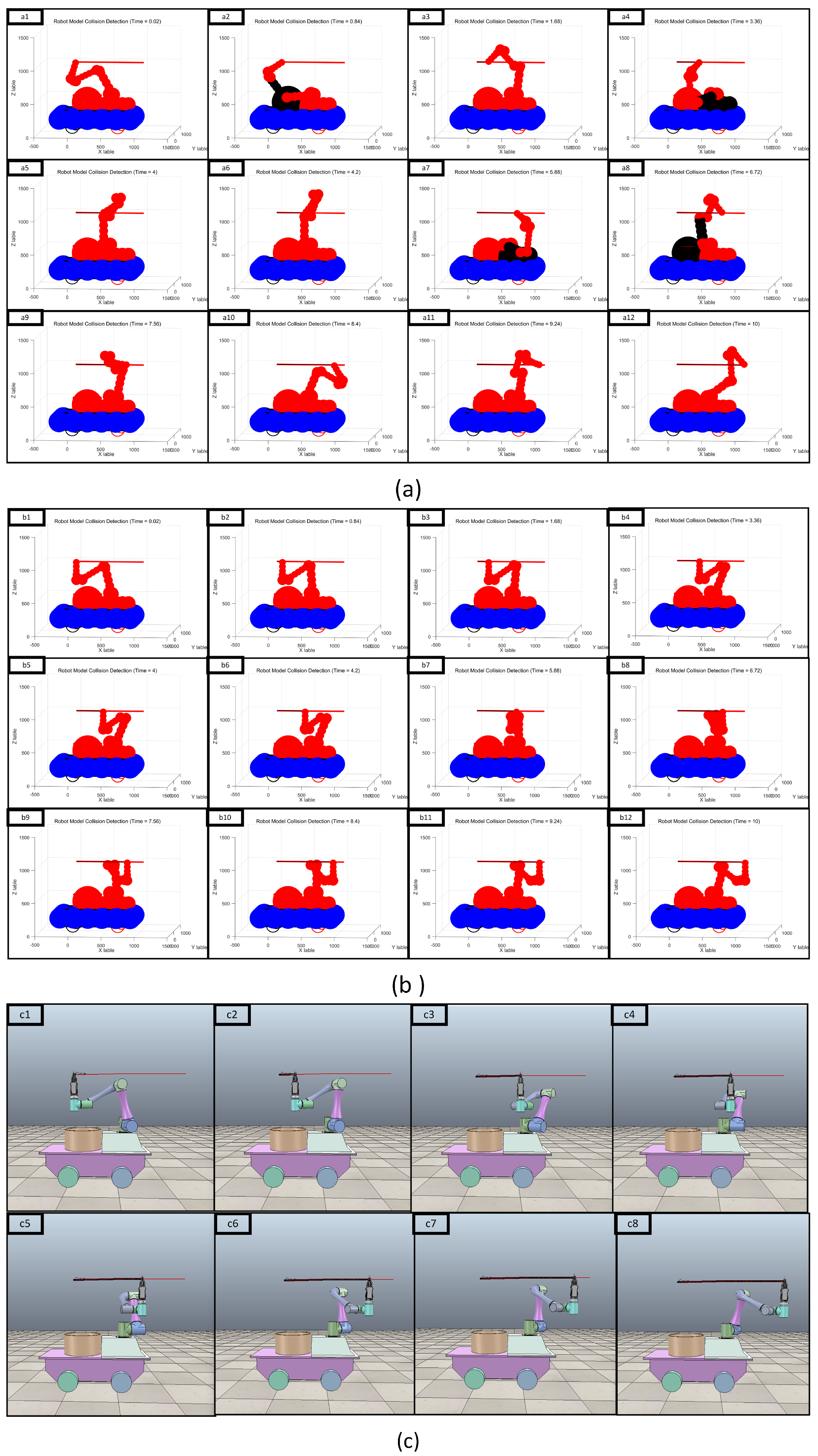
The mobile manipulator robot may not be able to completely arrive at the positions and postures required for a complex task. The following two reasons are the main causes for unreachable positions and posture: first, the actual position of the designated task may be outside the workspace of the mobile manipulator robot, and the current robot cannot perform trajectory tracking problems; second, the position and posture of the designated task are near the singular point of the mobile manipulator robot, and the typical control method cannot reach the location to complete the specified task. Regarding the first problem, researchers need to re-design and optimize the structure of the mobile manipulator robot; otherwise, no other method can address the first factor. However, we can effectively solve the second factor through the use of various swarm optimization algorithms. In actual practice, the success rate of the trajectory tracking task remains an effective evaluation criterion for comparing the performance of different optimization algorithms.
In solving trajectory tracking problems using population optimization algorithms, the DE algorithm has better performance than the other algorithm for solving specific tasks in terms of success rate. However, the success rate for solving the configuration parameters in the destined point based on the current DE algorithms cannot reach 100%, which can seriously affect the trajectory tracking accuracy. If we add collision avoidance into the trajectory tracking problem, the success rate for solving the configuration parameters in the destined point may be significantly reduced. To determine the influence of the success rate, we solve for the failed point whose position and posture are in the working space by performing multiple solutions based on the same DE algorithm. The multiple solutions show that the above-mentioned unreachable point can be reached again by re-solving, but the success rate will be lower than that of other locations. By comparing the specific solution process, we found that the initial population and the number of iterations are the main reasons for the failure of the above-mentioned task. Meanwhile, re-initialization of the population can significantly increase the success rate of the above-mentioned task compared to increasing the number of iterations. Furthermore, conducting the population initialization process again can significantly reduce the average time consumption for solving the configuration parameters for the destination point.
To ensure the accuracy of trajectory tracking, we re-initialize the population to track the failed point until the end effector reaches the specified point. In solving the trajectory tracking, we introduce the success index “ S u c ” added into the DE algorithm to improve the success rate. When the solution of any task point fails (“ S u c = 0 ”), we reset the initial population of the DE algorithm and continue to solve the configuration parameters of the current point. When the task point is successfully solved (“ S u c = 1 ”), we continue to solve the configuration parameters to reach the next task point.
(4) Optimized fitness function
When solving for the trajectory tracking based on the DE algorithm, the fitness function can sort the existing populations according to the requirements of actual motion. To solve the trajectory tracking of the mobile manipulator robot, we can directly combine multiple expressions to generate the fitness function, which takes a long time. To improve the solution speed of the DE algorithm, we must classify multiple expressions in trajectory tracking to construct different fitness functions for the DE algorithm.
In the DE algorithm, we decompose the trajectory tracking of the mobile manipulator into a constraint function and a termination function. The constraint function mainly sorts the optimal parameters that satisfy the basic requirements of the mobile manipulator, primarily including kinematic constraints and the shortest distance. The specific expression formula is:
f 1 ( q ) = W 1 i = 1 2 q m i + 1 q m i + W 2 i = 3 n q a i + 1 q a i + W 3 ( e x + e y + e z )
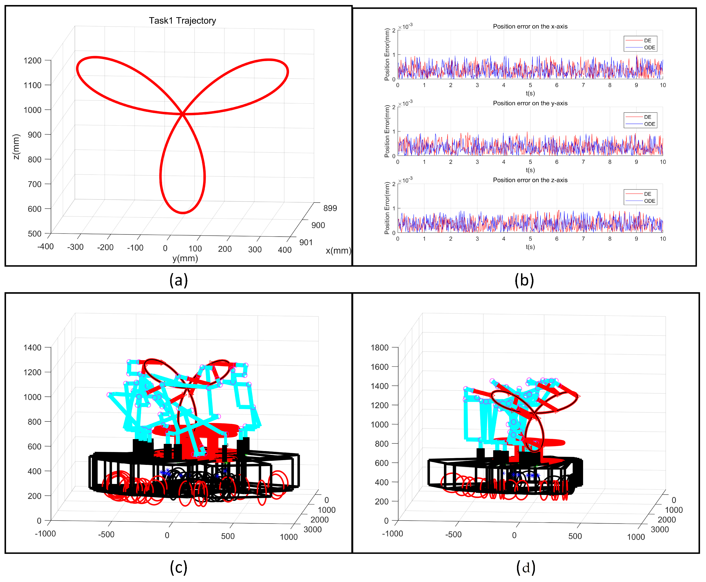
where the first term on the right of the formula represents the minimum motion of the mobile platform, the second term represents the minimum motion constraint of the manipulator robot, and the last term represents the position error of the end effector of the mobile manipulator robot.
The termination function is mainly used to select the best group in the population and jump out of the iterative operation of the DE algorithm. Therefore, the best optimization population needs to reach the designated position through the population. If the number of iterations is completely carried out, the population size will be increased, and the overall time-consuming exchange will become long. To improve the performance of the DE algorithm in solving the trajectory tracking problem of the mobile manipulator, we chose the collision-free constraint and the minimum position error for the final termination function. The specific expression is:
f 2 ( q ) = w 1 i = 1 ( e x + e y + e z ) + w 2 i = 1 ( o x + o y + o z ) f 3 ( q ) = c o l l i s i o n ( ) = 0
where the first term on the right of the top formula indicates the position error of the end effector, the second term indicates the posture error of the end effector, f 2 ( ) indicates whether the robot meets the basic requirements of the trajectory tracking, and f 3 ( q ) = 0 indicates that the robot does not collide.

3.3. Solving the Trajectory Tracking Problem

In order to solve the tracking problem for the mobile manipulator robot, we established an optimal problem under multiple constraints based on the various actual limitations and task requirements. Then, we optimized the typical differential evolution algorithm in various aspects in order to improve the efficiency in solving the optimal problem. Therefore, we realized the trajectory tracking of mobile manipulator robot by re-defining the trajectory tracking problem and optimizing the differential evolution algorithm. In order to demonstrate the solution process more concisely, the flow chart for solving the trajectory tracking problem based on the optimized differential evolution algorithm is shown in Figure 2.
To understand the optimization of the DE algorithm detailed in the above subsection, we summarize the specific steps of the optimized DE algorithm used to solve the trajectory tracking problem for the mobile manipulator. The detailed steps of the optimized DE algorithm are illustrated in the following, and the flow chart is shown in Figure 3.
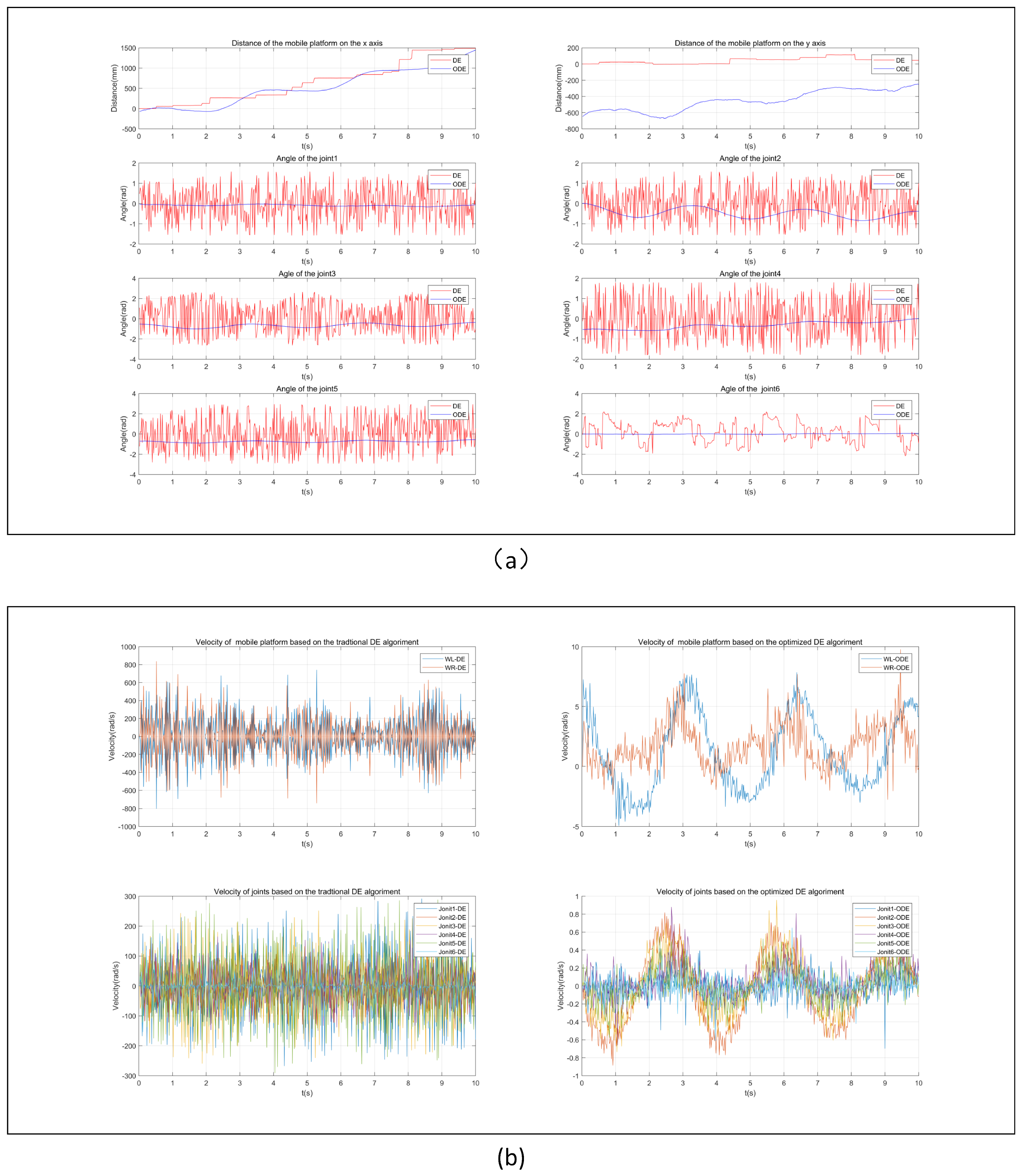
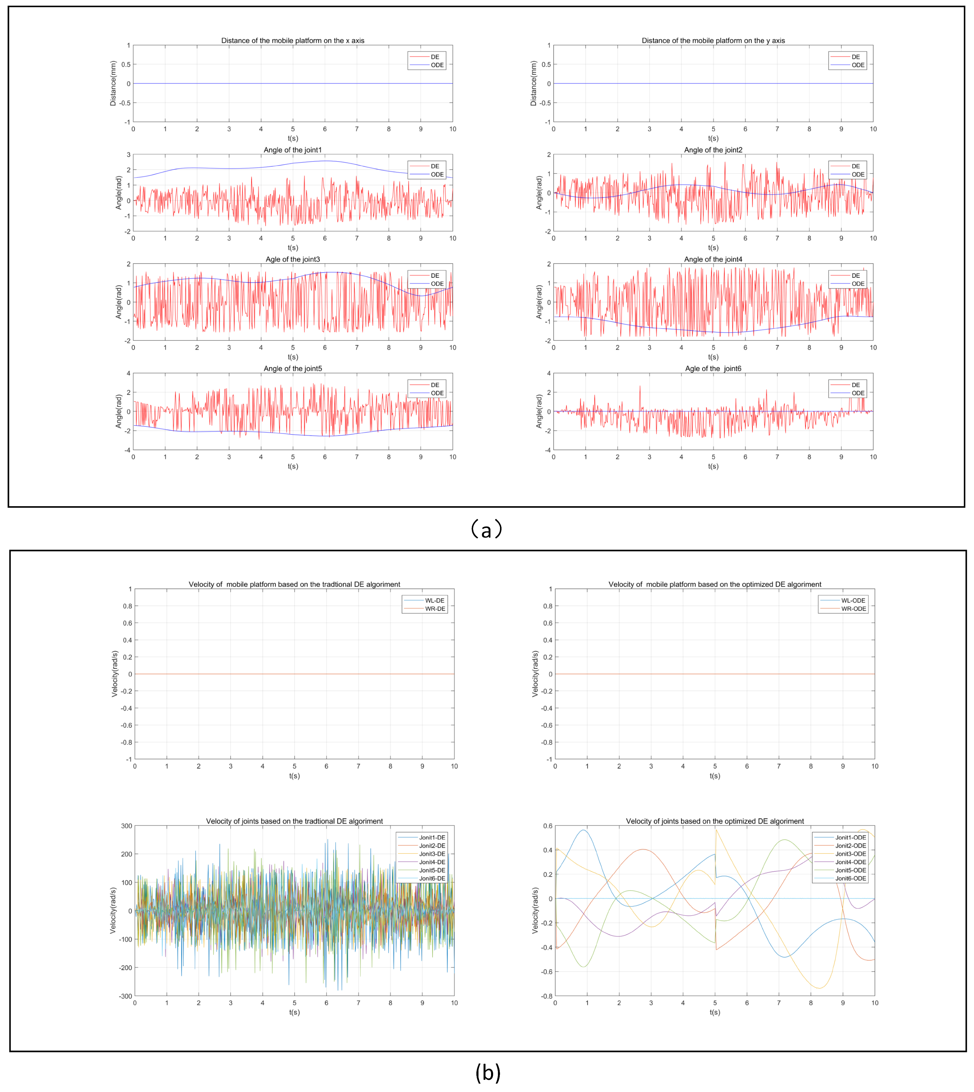
Step 1: Specify task. Obtain the position and posture for the trajectory tracking task according to the actual requirements; determine the motion time, and set the success rate to S u c = 0 .
Step 2: Enter the loop for solving the trajectory tracking.
Step 3: Initialize key parameters. Set the initial population as N P , the maximum number of iterations as G, the dimensionality of the trajectory tracking problem (i.e., the number of driving joints) as D, the variation factor parameter as F, and the crossover rate as C R .
Step 4: Initialization operation. (1) Randomly assign values to the population for initialization operations based on the speed constraint (28) and add the opposing population generated by the inverse learning method (29) into the initial population. (2) Re-initialize the basic population considering the angle constraints (30) of the mobile manipulator robot. (3) Solve the fitness function (34) or (35) of the re-initialized population and sort the population based on the fitness values.
Step 5: Mutation operation. (1) Generate the first new population based on the corresponding mutation function (31) after randomly selecting three populations ( r 1 , r 2 , r 3 , and b e ). (2) Form the second new population, which meets the speed constraint, using Equation (32). (3) Form the third new population, which satisfies the angle constraint, based on Equation (33).
Step 6: Crossover operation. Determine the crossover population through Equation (26).
Step 7: Selection operation. Determine the best population through the best fitness function after obtaining the fitness values.
Step 8: Judgment operation. (1) Carry out collision detection on the best population in order to determine whether collisions will occur. (2) Perform error judgment on the best population in order to determine whether the end effector can reach the designated position and posture. (3) Determine whether the solution meets the conditions obtained through the termination function. When the solution is successful, the DE algorithm will jump out of the loop and set the index S u c = 1 ; otherwise, it continues to solve the trajectory tracking until finishing the iteration and sets the index to S u c = 0 .
Step 9: Process results. Determine whether to save the solution data of the task based on the index state ( S u c ). When S u c = 1 , the joint angle is saved, and the time is incremented to track the following point; otherwise, the system jumps to Step 3.
Step 10: End the loop. Judge whether the final target point has been reached. If the end effector has reached the point, the optimized DE algorithm completes the solution of the trajectory tracking problem; otherwise, the DE algorithm continues to solve the trajectory tracking problem.

4. Simulation Results

In this section, various simulations are designed to demonstrate the performance of the optimized differential evolution method in order to solve the trajectory tracking problem for the mobile manipulator. We chose the mobile manipulator depicted in Figure 1 as the research object with the mobile platform adopting differential driving control and the manipulator sub-system having six degrees of freedom. The specific parameters of the mobile manipulator robot can be found in the article [30]. During the movement of the mobile manipulator robot, there was no position constraint on the control parameter of the mobile platform, but the joints of the manipulator robot had angle limitations in their actual movements. Meanwhile, the speed of the driving wheels of the mobile platform were subject to speed constraints. The speeds of the corresponding joints of the manipulator robot also had range constraints.Therefore, the whole control parameters of the mobile manipulator had speed constraints, which can be expressed as:
C a n g : q L = [ , , 180 , 169 , 165 , 150 , 102 . 5 , 167 . 5 , 167 . 5 ] ; q U = [ + , + , + 180 , + 169 , + 165 , + 150 , + 102 . 5 , + 167 . 5 , + 167 . 5 ] ; C v e l : q ˙ L = [ 10 , 10 , π 2 , π 2 , π 2 , π 2 , π 2 , π 2 , π 2 ] ; q ˙ U = [ + 10 , + 10 , + π 2 , + π 2 , + π 2 , + π 2 , + π 2 , + π 2 , + π 2 ] ;
where C a n g indicates the angle constraint of these whole control parameters of the mobile manipulator robot, and C v e l represents the corresponding speed constraint of these control parameters.
To verify the performance of the optimized differential evolution algorithm, we used a personal computer to complete various trajectory tracking experiments. The basic configuration of the computer was an Intel Core i5-7500, CPU @ 3.4 Hz, and RAM @ 8 GB, which is suitable for practical applications. For the first simulation, we designed a simple trajectory tracking task including a position requirement in order to compare the basic performance of the optimized DE method proposed in this paper with the typical DE algorithm. This simulation was intended to prove that the optimized DE algorithm proposed in this paper can satisfactorily meet the various constraints of the mobile manipulator. For the second experiment, we designed a complex trajectory tracking task including position and posture requirements in order to compare the permanence of the optimized DE algorithm with the typical DE algorithm and to prove the effectiveness of the improvements proposed in this paper, as well as the superior performance of the optimized DE algorithm.

4.1. Trajectory Tracking Task Considering the Posture Requirements

In this section, we mainly compare the basic performance of the optimized DE algorithm with that of the typical DE algorithm in solving simple trajectory tracking tasks. We designed two different trajectories only considering position requirements for the mobile manipulator. The main test contents included whether trajectory tracking was completed (100% success rate), whether collision-free motion was achieved, and whether the speed and angle constraints were satisfied.
To complete these simple trajectory tracking tasks, the paper set the total motion time as T s = 10 s and the sampling time as d t = 0.02 s, and the number of sampling point is N = 500 . In initializing the parameters of the differential evolution (DE) algorithm, we set each key parameter as follows, addedin order to track the above four different trajectories, including: The size of the population was N P = 50 , the number of iterations was G = 1000 , the variation factor was F = 0.5 , and the crossover probability was C R = 0.9 . The typical DE algorithm and optimized DE algorithm were used for experimental simulation to obtain the tracking results for these different trajectories. These specific trajectories can be expressed as follows:
Task 1: The first trajectory was a three-petal flower in the Y Z plane, expressed as:
x = 900 ; y = 200 sin 4 π N k + 200 cos 2 π N k , ( k = 1 : 500 ) ; z = 920 + 200 sin 2 π N k + 200 cos 4 π N k ;
Task 2: The second trajectory was a spiral in three-dimensional space, which can be described as:
x = 572 + 2000 N k , ( k = 1 : 500 ) ; y = 300 sin 6 π N k ; z = 920 + 300 cos 6 π N k ;
Figure 4a and Figure 5a show the expected trajectories for completing Tasks 1 and 2, respectively. Task 1 follows a simple motion trajectory in two-dimensional space, while Task 2 follows a more complex trajectory in three-dimensional space. We used the typical DE algorithm and the optimized DE algorithm to track these trajectories. The tracking errors for the first and second trajectories are shown in Figure 4b and Figure 5b, respectively. It can be seen both these position errors fully met the trajectory error requirements. Therefore, these algorithms can drive the mobile manipulator’s end effector along the expected trajectory in either a two- or three-dimensional space.
The tracking results for Tasks 1 and 2, based on the typical DE algorithm and the optimized DE algorithm, are shown in Figure 4c,d and Figure 5c,d, respectively. The basic structure of the mobile manipulator robot at the corresponding positions based on these algorithms for tracking the first trajectory is also shown in Figure 6a–c and Figure 7a–c. The mobile manipulator robot with the configuration for tracking the first trajectory solved based on the typical DE algorithm presented a collision, marked in black in Figure 6(a5). Furthermore, the robot with the configuration for tracking the second trajectory solved based on the typical DE algorithm also collided with itself, as shown in Figure 7(a2). However, the robot with the configuration for the first and the second trajectories solved based on the optimized DE algorithm did not present any collisions. Figure 8 and Figure 9 show the mobile manipulator’s corresponding position and the speed of each driving joint when tracking the first and second trajectories. When tracking these trajectories using the typical DE algorithm, the angle and speed of the driving joint of the mobile manipulator robot presented large jumps, meaning that it could not meet the realistic requirements. Meanwhile, the optimized DE algorithm could reduce the change in the angle and speed to meet the motor’s physical constraints through the addition of angle and speed constraints.
Based on the trajectory tracking results for the mobile manipulator obtained with the typical DE and the optimized DE algorithms, we derived the following conclusions:
(1) Comparing the trajectory tracking errors shown in Figure 4b and Figure 5b, the trajectory error for each task based on the typical DE algorithm was similar to that obtained by the optimized DE algorithm. Furthermore, the trajectory tracking tasks could be achieved by both the traditional and optimized DE algorithms.
(2) Comparing the basic configuration for the trajectory tracking task shown in Figure 6a–c and Figure 5a–c, these configurations based on the traditional DE algorithm must have a collision, as shown in Figure 6(a5) and Figure 7(a2). Considering these self-collisions, the mobile manipulator robot based on the typical DE algorithm cannot reach these specified points in order to continue completing these tasks. With the self-collision detection function and the success rate added into the optimized DE algorithm, we can ensure that the mobile manipulator system does not collide at these specified points. Therefore, the optimized DE algorithm can effectively pass the specified location to ensure the smooth movement of the mobile manipulator robot, as shown in Figure 6(c1–c8) and Figure 7(c1–c8).
(3) Comparing the speed and angle of each driving joint in completing the trajectory tracking task shown in Figure 8 and Figure 9, both the traditional DE algorithm and the optimized DE algorithm can meet the specified angle limitations for each driving joint. However, the typical DE algorithm could not meet the speed constraint of each driving joint, as shown in Figure 8b and Figure 9b. Meanwhile, the optimized DE algorithm met the actual requirements of the driving joints by adding joint and speed limitations into the initial configuration and mutation operations.
Comparing the performances of the typical DE algorithm and the optimized DE algorithm for solving these simple trajectory tasks, the optimized DE algorithm effectively avoided self-collision during movement through the added success index and collision detection function. Meanwhile, the optimized DE algorithm also ensured that the result of the trajectory tracking met the speed constraint and angle constraint.

4.2. Trajectory Tracking Task Considering Position and Posture Requirements

Next, we tested the performance of the proposed DE algorithm with that of the typical DE algorithm in terms of solving the complex trajectory tracking problem. The main test included whether trajectory tracking could be completed (100% success rate), collision-free motion could be achieved, and the speed and angle constraints could be satisfied. To prove that the proposed optimized DE algorithm is more suitable for the practical application of a mobile manipulator, we designed two different trajectories to test the performance of the optimized DE algorithm in solving the trajectory tracking problem of the mobile manipulator. We set the overall motion time as T s = 10 s and the sampling time as d t = 0.02 s. In the process of initializing the parameters of the differential evolution (DE) algorithm, we set each key parameter as follows: the size of the population was N P = 50 , the number of iterations was G = 1000 , the variation factor was F = 0.5 , and the crossover probability was C R = 0.9 . We used the two different motion trajectories, as detailed below. The typical DE algorithm and the optimized DE algorithm were used in the experimental simulation in order to obtain the results of tracking different trajectories. The specific trajectories can be expressed as:
Task 3: The third trajectory was a line trajectory in the X Z plane, but the end effector of the robot had to be held vertically upward from the X Y plane. The position of the third trajectory can be expressed as:
x = 53.1 + 2.0378 k , ( k = 1 : 500 ) ; y = 241 ; z = 1068.2 ;
Task 4: The fourth trajectory was a double closed-loop arc in three-dimensional space, but the end effector of the robot had to be held inward, perpendicular to the Y Z plane. The position of the fourth trajectory can be described as:
x 1 = 600 + 400 N · k , ( k = 1 : 250 ) ; x 2 = 1000 400 N · k , ( k = 251 : 500 ) ; y = 150 sin 4 π N k z = 1220 + 150 cos 2 π N k
In summary, Task 3 was a line in a three-dimensional space, while Task 4 was a complex trajectory in three-dimensional space. Both of these tasks require position and posture requirements to be taken into consideration. Figure 10a and Figure 11a show the results of trajectory tracking for the mobile manipulator for Tasks 3 and 4, respectively. Figure 10b and Figure 11b show the tracking errors for these trajectories, respectively, for the typical and optimized DE algorithms. In these figures, the position error in the three axes was within 10 3 mm, thus fully meeting the error requirement. According to these tracking errors, these two DE algorithms effectively achieved the trajectory tracking task.
Figure 10c,d and Figure 11c,d detail the trajectory tracking results obtained using the typical and optimized DE algorithms for Tasks 3 and 4, respectively. The mobile manipulator robot in the configuration for completing Task 3 solved based on the typical DE algorithm sustained a collision, marked in black in Figure 12(a2,a4,a7,a8), and the robot in the configuration for completing Task 4 solved by the same algorithm also collided with itself, marked in black in Figure 13(a6,a10). Meanwhile, the robot’s end effector at the same position as the solved configuration based on the optimized DE algorithm did not collide with itself when completing either the third or fourth tasks. We also obtained the changes in the angle and speed of the driving joints for completing Task 3 and Task 4, as shown in Figure 14a,b and Figure 15a,b. The changes in angles for each joint obtained by the optimized DE algorithm were small. Additionally, the change in speed was much smaller than that in the corresponding solution based on the traditional DE algorithm. Therefore, based on the optimized DE algorithm, the results met the physical constraints of the mobile manipulator robot. Overall, the optimized DE algorithm was found to be more suitable for completing the trajectory tracking of the mobile manipulator robot than the typical DE algorithm.
Comparing the results for the complex trajectory tracking problem of the mobile manipulator before and after optimizing the DE algorithm, we came to the following conclusions:
(1) Comparing the trajectory tracking errors shown in Figure 10b and Figure 11b, the average error of each trajectory based on the traditional DE algorithm was more significant than that for the optimized DE algorithm. The maximum position error of the trajectories based on the traditional DE algorithm was also much greater than the specified error range. However, the maximum error for the optimized DE algorithm met the error requirements. Therefore, the optimized DE algorithm presents better performance in solving the trajectory tracking problem.
(2) Comparing the success rate of trajectory tracking in Figure 10c,d and Figure 11c,d, it can be seen that the success rate of the optimized DE algorithm could reach 100% by taking into account the error and collision constraints. However, the success rate of the typical DE algorithm was relatively low compared to the optimized DE algorithm. Therefore, the optimized DE algorithm can reduce the trajectory error and, thus, improve the performance over the DE algorithm in solving the complex trajectory tracking problem for a mobile manipulator robot.
(3) Comparing the results of the mobile manipulator in the trajectory tracking task shown in Figure 12a–c and Figure 13a–c, we can see that the configuration of the driving joints solved by the traditional DE algorithm presented collisions in Figure 12(a2,a4,a7,a8) and Figure 13(a6,a10). With the self-collision detection function added to the DE algorithm, it was ensured that the mobile manipulator system did not self-collide at these specified points. Therefore, the optimized DE algorithm can effectively pass the specified points and ensure the smooth movement of the mobile manipulator robot, as shown in Figure 12(c1–c8) and Figure 13(c1–c8).
(4) Comparing the speed and angle of each driving joint in completing the trajectory tracking task, as shown in Figure 14 and Figure 15, the optimized DE algorithm obtained smaller changes in each joint angle at adjacent moments. Furthermore, the optimized DE algorithm met the actual requirements of the driving joints by adding angle and speed limitations into the initial configuration and mutation operations.
According to the above comparison results, we demonstrated that the optimized differential evolution algorithm proposed in this study is more suitable for allowing mobile manipulators to track complex trajectories, especially when taking both position and posture requirements into consideration.

5. Conclusions

In this study, we transformed the trajectory tracking problem for a mobile manipulator into an optimization problem under multiple constraints. Considering the actual movement of the mobile manipulator robot, we developed equations and inequalities to express various constraints, including joint speed, joint angle, self-collision, and motion constraints. The re-definition of the trajectory tracking problem can effectively avoid the need for the inverse solution of the Jacobian matrix in the velocity layer, as well as ensuring that the manipulator’s end effector can pass singular positions smoothly. Then, a new differential evolution algorithm was applied to solve the optimization problem under multiple constraints, and we optimized the critical steps of the typical differential evolution algorithm based on these constraints to improve the trajectory tracking performance of the mobile manipulator robot. Meanwhile, the optimized differential evolution algorithm can ensure that the end of the manipulator can pass singular positions smoothly, improve the success rate of the solution, and realize the high-precision trajectory tracking of the mobile manipulator robot without self-collisions. Overall, the optimized DE algorithm outperformed the typical DE algorithm in solving trajectory tracking problems for mobile manipulator robots.
The trajectory tracking problem for mobile manipulators is a fundamental problem for achieving specified tasks, in which the design of a motion trajectory is also a pre-requisite for completing the task. Therefore, in future research, we intend to study various intelligent algorithms in order to plan the most suitable trajectory for the mobile manipulator robot.

Author Contributions

Conceptualization, L.Q.; methodology, L.Q.; software, X.L. and Q.L.; validation, L.Q., X.L. and Q.L.; formal analysis, L.Q., X.L. and Q.L.; investigation, L.Q., X.L. and Q.L.; resources, L.Q., X.L. and Q.L.; data curation, L.Q., X.L. and Q.L.; writing—original draft preparation, Q.L.; writing—review and editing, Q.L., X.L. and Q.L.; visualization, L.Q., X.L. and Q.L.; supervision, L.Q., X.L. and Q.L.; project administration, X.L. and Q.L. All authors have read and agreed to the published version of the manuscript.

Funding

This research received no external funding.

Institutional Review Board Statement

Not applicable.

Informed Consent Statement

Not applicable.

Data Availability Statement

Not applicable.

Acknowledgments

Not applicable.

Conflicts of Interest

The authors declare no conflict of interest.

References

  1. Schepper, D.D.; Moyaers, B.; Schouterden, G.; Kellens, K.; Demeester, E. Towards robust human-robot mobile co-manipulation for tasks involving the handling of non-rigid materials using sensor-fused force-torque, and skeleton tracking data. Procedia CIRP 2020, 97, 325–330. [Google Scholar] [CrossRef]
  2. Li, M.; Yang, Z.; Zha, F.; Wang, X.; Wang, P.; Li, P.; Ren, Q.; Chen, F. Design and analysis of a whole-body controller for a velocity controlled robot mobile manipulator. Sci. China Inf. Sci. 2020, 63, 170204. [Google Scholar] [CrossRef]
  3. Recker, T.; Heilemann, F.; Raatz, A. Handling of large and heavy objects using a single mobile manipulator in combination with a roller board. Procedia CIRP 2020, 97, 21–26. [Google Scholar] [CrossRef]
  4. Zhang, H.; Sheng, Q.; Sun, Y.; Sheng, X.; Xiong, Z.; Zhu, X. A novel coordinated motion planner based on capability map for autonomous mobile manipulator. Robot. Auton. Syst. 2020, 129, 103554. [Google Scholar] [CrossRef]
  5. Qiu, C.; Cao, Q. Modeling and analysis of the dynamics of an omni-directional mobile manipulators system. J. Intell. Robot. Syst. Theory Appl. 2008, 52, 101–120. [Google Scholar] [CrossRef]
  6. Khan, A.T.; Li, S.; Cao, X. Control framework for cooperative robots in smart home using bio-inspired neural network. Meas. J. Int. Meas. Confed. 2021, 167, 108253. [Google Scholar] [CrossRef]
  7. Zhong, G.; Kobayashi, Y.; Hoshino, Y.; Emaru, T. System modeling and tracking control of mobile manipulator subjected to dynamic interaction and uncertainty. Nonlinear Dyn. 2013, 73, 167–182. [Google Scholar] [CrossRef]
  8. Dietrich, A.; Bussmann, K.; Petit, F.; Kotyczka, P.; Ott, C.; Lohmann, B.; Albu-Schäffer, A. Whole-body impedance control of wheeled mobile manipulators: Stability analysis and experiments on the humanoid robot Rollin’ Justin. Auton. Robot. 2016, 40, 505–517. [Google Scholar] [CrossRef] [Green Version]
  9. Li, W.; Xiong, R. Dynamical Obstacle Avoidance of Task- Constrained Mobile Manipulation Using Model Predictive Control. IEEE Access 2019, 7, 88301–88311. [Google Scholar] [CrossRef]
  10. Fan, Q.; Gong, Z.; Zhang, S.; Tao, B.; Yin, Z.; Ding, H. A vision-based fast base frame calibration method for coordinated mobile manipulators. Robot. Comput. Integr. Manuf. 2020, 68, 102078. [Google Scholar] [CrossRef]
  11. Fan, Q.; Gong, Z.; Tao, B.; Gao, Y.; Yin, Z.; Ding, H. Base position optimization of mobile manipulators for machining large complex components. Robot. Comput. Integr. Manuf. 2021, 70, 102138. [Google Scholar] [CrossRef]
  12. Karami, A.; Sadeghian, H.; Keshmiri, M.; Oriolo, G. Hierarchical tracking task control in redundant manipulators with compliance control in the null-space. Mechatronics 2018, 55, 171–179. [Google Scholar] [CrossRef]
  13. Galicki, M. Inverse Kinematics Solution to Mobile Manipulators. Int. J. Robot. Res. 2003, 22, 1041–1064. [Google Scholar] [CrossRef]
  14. Xiao, L.; Liao, B.; Li, S.; Zhang, Z.; Ding, L.; Jin, L. Design and Analysis of FTZNN Applied to the Real-Time Solution of a Nonstationary Lyapunov Equation and Tracking Control of a Wheeled Mobile Manipulator. IEEE Trans. Ind. Inform. 2018, 14, 98–105. [Google Scholar] [CrossRef]
  15. Ram, R.V.; Pathak, P.M.; Junco, S.J. Inverse kinematics of mobile manipulator using bidirectional particle swarm optimization by manipulator decoupling. Mech. Mach. Theory 2019, 131, 385–405. [Google Scholar] [CrossRef]
  16. Xiao, L.; Zhang, Y. Solving time-varying inverse kinematics problem of wheeled mobile manipulators using Zhang neural network with exponential convergence. Nonlinear Dyn. 2014, 76, 1543–1559. [Google Scholar] [CrossRef]
  17. Tchoń, K. Repeatable, extended Jacobian inverse kinematics algorithm for mobile manipulators. Syst. Control Lett. 2006, 55, 87–93. [Google Scholar] [CrossRef]
  18. Tchoń, K.; Jakubiak, J. Extended Jacobian inverse kinematics algorithm for nonholonomic mobile robots. Int. J. Control 2006, 79, 895–909. [Google Scholar] [CrossRef]
  19. Zhang, Y.; Li, W.; Zhang, Z. Physical-limits-constrained minimum velocity norm coordinating scheme for wheeled mobile redundant manipulators. Robotica 2015, 33, 1325–1350. [Google Scholar] [CrossRef] [Green Version]
  20. Zhang, Y.; Yan, X.; Chen, D.; Guo, D.; Li, W. QP-based refined manipulability-maximizing scheme for coordinated motion planning and control of physically constrained wheeled mobile redundant manipulators. Nonlinear Dyn. 2016, 85, 245–261. [Google Scholar] [CrossRef]
  21. Kong, Y.; Zhang, R.; Jiang, Y.; Xia, X.; Wei, C. A Repeatable Optimization for Kinematic Energy System with Its Mobile Manipulator Application. Complexity 2019, 2019, 8642027. [Google Scholar] [CrossRef] [Green Version]
  22. Khan, A.H.; Li, S.; Chen, D.; Liao, L. Tracking control of redundant mobile manipulator: An RNN based metaheuristic approach. Neurocomputing 2020, 400, 272–284. [Google Scholar] [CrossRef]
  23. Rokbani, N.; Alimi, A.M. Inverse kinematics using particle swarm optimization, a statistical analysis. Procedia Eng. 2013, 64, 1602–1611. [Google Scholar] [CrossRef] [Green Version]
  24. Sancaktar, I.; Tuna, B.; Ulutas, M. Inverse kinematics application on medical robot using adapted PSO method. Eng. Sci. Technol. Int. J. 2018, 21, 1006–1010. [Google Scholar] [CrossRef]
  25. Hernandez-Barragan, J.; Lopez-Franco, C.; Arana-Daniel, N.; Alanis, A.Y. Inverse kinematics for cooperative mobile manipulators based on self-adaptive differential evolution. PeerJ Comput. Sci. 2021, 7, e419. [Google Scholar] [CrossRef] [PubMed]
  26. Filho, P.P.R.; Suane, S.P.; Praxedes, V.N.; Hemanth, J.; de Albuquerque, V.H.C. Control of singularity trajectory tracking for robotic manipulator by genetic algorithms. J. Comput. Sci. 2019, 30, 55–64. [Google Scholar] [CrossRef]
  27. Zhang, Q.; Wang, D.; Gao, L. Research on the inverse kinematics of manipulator using an improved self-adaptive mutation differential evolution algorithm. Int. J. Adv. Robot. Syst. 2021, 18, 17298814211014413. [Google Scholar] [CrossRef]
  28. Ayyıldız, M.; Çetinkaya, K. Comparison of four different heuristic optimization algorithms for the inverse kinematics solution of a real 4-DOF serial robot manipulator. Neural Comput. Appl. 2016, 27, 825–836. [Google Scholar] [CrossRef]
  29. López-Franco, C.; Hernández-Barragán, J.; Alanis, A.Y.; Arana-Daniel, N.; López-Franco, M. Inverse kinematics of mobile manipulators based on differential evolution. Int. J. Adv. Robot. Syst. 2018, 15, 1729881417752738. [Google Scholar] [CrossRef] [Green Version]
  30. Qiao, L.; Luo, X.; Luo, Q.; Li, M.; Jiang, J. Optimizing Kinematic Modeling and Self-Collision Detection of a Mobile Manipulator Robot by Considering the Actual Physical Structure. Appl. Sci. 2021, 11, 10591. [Google Scholar] [CrossRef]
Figure 1. Illustration of a mobile manipulator robot: (a) Physical structure of the mobile manipulator; (b) Critical coordinate frames of the mobile manipulator.
Machines 10 01232 g001
Figure 2. Flowchart for trajectory tracking problem solution.
Machines 10 01232 g002
Figure 3. Flowchart of the optimized DE algorithm.
Machines 10 01232 g003
Figure 4. Simulation results for Task 1: (a) The trajectory designated for task 1; (b) Tracking error for the first trajectory; (c) Motion of the robot based on the typical DE algorithm; (d) Motion of the robot based on the optimized DE algorithm.
Machines 10 01232 g004
Figure 5. Simulation results for Task 2: (a) The trajectory designated for task 2; (b) Tracking error for the second trajectory; (c) Motion of the robot based on the typical DE algorithm; (d) Motion of the robot based on the optimized DE algorithm.
Machines 10 01232 g005
Figure 6. Configuration results of mobile manipulator robot for Task 1: (a1a12) Basic structure of the robot at different moments based on the typical DE algorithm; (b1b12) Basic structure of the robot at different moments based on the optimized DE algorithm; (c1c8) Actual structure of the robot based on the optimized DE algorithm.
Machines 10 01232 g006
Figure 7. Configuration results of mobile manipulator robot for Task 2: (a1a12) Basic structure of the robot at different moments based on the typical DE algorithm; (b1b12) Basic structure of the robot at different moments based on the optimized DE algorithm; (c1c8) Actual structure of the robot based on the optimized DE algorithm.
Machines 10 01232 g007
Figure 8. Motion of the mobile manipulator robot in the first task: (a) Joint angles of the mobile manipulator robot for the first trajectory; (b) Joint velocity of the mobile manipulator robot for the first trajectory.
Machines 10 01232 g008
Figure 9. Motion of the mobile manipulator robot in the second task: (a) Joint angles of the mobile manipulator robot for the second trajectory; (b) Joint velocity of the mobile manipulator robot for the second trajectory.
Machines 10 01232 g009
Figure 10. Simulation results for Task 3: (a) The trajectory designated for Task 3; (b) Tracking error of the third trajectory; (c) Motion of the robot based on the typical DE algorithm; (d) Motion of the robot based on the optimized DE algorithm.
Machines 10 01232 g010
Figure 11. Simulation results for Task 4: (a) The trajectory designated for Task 4; (b) Tracking error of the fourth trajectory; (c) Motion of the robot based on the typical DE algorithm; (d) Motion of the robot based on the optimized DE algorithm.
Machines 10 01232 g011
Figure 12. Configuration results of mobile manipulator robot for Task 3: (a1a12) Basic structure of the robot at different moments based on the typical DE algorithm; (b1b12) Basic structure of the robot at different moments based on the optimized DE algorithm; (c1c8) Actual structure of the robot based on the optimized DE algorithm.
Machines 10 01232 g012
Figure 13. Configuration results of mobile manipulator robot for Task 4: (a1a12) Basic structure of the robot at different moments based on the typical DE algorithm; (b1b12) Basic structure of the robot at different moment based on the optimized DE algorithm; (c1c8) Actual structure of the robot based on the optimized DE algorithm.
Machines 10 01232 g013
Figure 14. Motion of the mobile manipulator robot in the third task: (a) Joint angles of the mobile manipulator robot for the third trajectory; (b) Joint velocity of the mobile manipulator robot for the third trajectory.
Machines 10 01232 g014
Figure 15. Motion of the mobile manipulator robot in the fourth task: (a) Joint angles of the mobile manipulator robot for the fourth trajectory; (b) Joint velocity of the mobile manipulator robot for the fourth trajectory.
Machines 10 01232 g015
Publisher’s Note: MDPI stays neutral with regard to jurisdictional claims in published maps and institutional affiliations.

