1. Introduction
Compared with the parallel manipulators (PMs) without actuation redundancy, the redundantly actuated PMs have some advantages, such as higher stiffness and fewer singular configurations [
1,
2,
3], and thus they are suitable for applications requiring high accuracy. In general, the methods for producing redundantly actuated PMs can be divided into two categories [
4]: one is to replace some passive kinematic joints in the limbs with the actuated ones, and the other is to add one or more actuated limbs to the original PM, but the characteristics of the output motion stay the same. Because of the advantages of the second type with better force distributions [
5,
6], this paper focuses on the redundantly actuated PMs with more limbs.
Elastostatic stiffness modeling and the performance evaluation of the PMs with actuation redundancy are necessary for the design stage. The goal of the elastostatic stiffness modeling of PMs is to create a mapping between the deformations of the moving platform and the external loads in the reachable workspace [
7]. The stiffness characteristics can be obtained from the stiffness matrices of all the components and PM. Many works on the stiffness modeling of PMs have been carried out, which can be mainly divided into two types: finite element analysis (FEA) [
8,
9,
10,
11,
12], and analytical modeling [
13,
14,
15,
16,
17,
18,
19,
20,
21,
22,
23,
24,
25,
26,
27,
28,
29,
30,
31]. Some scholars, such as Fauroux et al. [
9,
10,
11] and Klimchik et al. [
12], have adopted the FEA method to conduct some stiffness analysis. Based on the FEA method, the deformation information of corresponding configurations can be obtained directly by using some FEA software, such as ANSYS. However, it should be noted that the deformation of different configurations can only be calculated sequentially, and the process is time-consuming [
13,
14]. Regarding analytical modeling, a great deal of research has been conducted by scholars such as Gosselin [
16], Zhang et al. [
17,
18,
19], Lipkin et al. [
20], Kumar et al. [
21,
22,
23], Pashkevich et al. [
13], Portman et al. [
26,
27], Ding et al. [
29], and so on. Considering the compliance of actuated joints, Gosselin [
16] developed the mapping relationship between the forces and deformations of PMs. Zhang et al. [
17,
18,
19] considered the compliance of the actuated joints and links and analyzed the stiffness of PMs. Lipkin et al. [
20] analyzed the stiffness of the compliant system with some external loads and obtained the asymmetric stiffness matrix. Pashkevich et al. [
13] investigated the overconstrained PMs with compliant actuated joints and flexible links and obtained a relatively accurate stiffness matrix. Based on the Lie-group theory and screw theory, Ding and his co-workers [
29] developed a theoretical method to analyze the accuracy of the redundantly actuated and overconstrained PMs that takes the actuated errors and internal elastic forces into account. In addition to the above work, researchers have also carried out many explorations into the theoretical stiffness modeling of PMs.
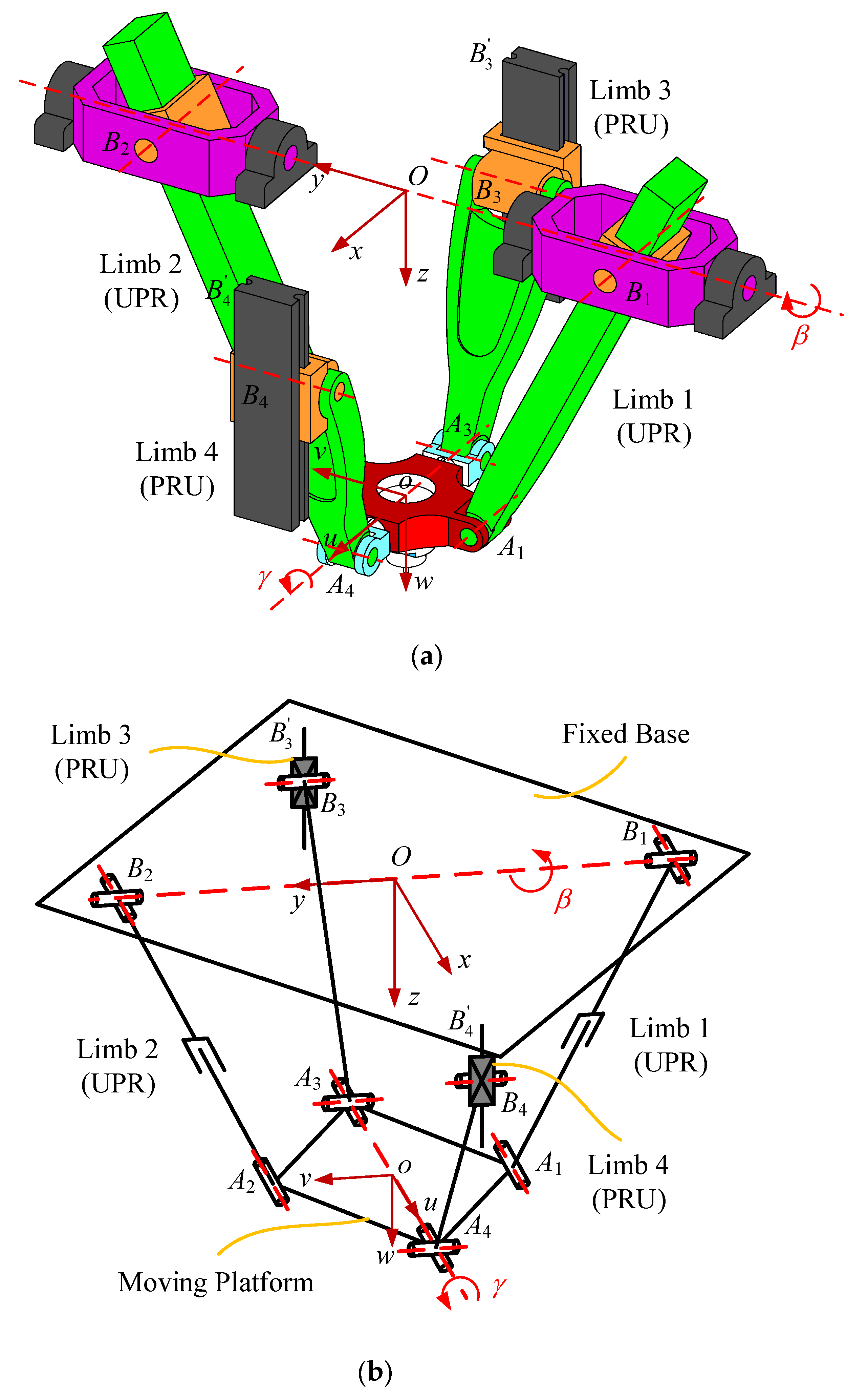
This paper presents a systematic elastostatic stiffness modeling and performance analysis of a redundantly actuated 2UPR–2PRU PM [
32]. The 2UPR–2PRU PM with actuation redundancy is a PM with two rotational and one translational degrees of freedom (DoFs), which has potential for the machining of curved workpieces with high precision. In this paper, the analytical stiffness modeling method based on the strain energy [
33,
34] is used. The elastostatic stiffness matrices of limbs and the overall PM can be easily developed by utilizing the principle of strain energy. All the results in the stiffness analysis have intuitive forms of expression and clear physical meanings. Based on this stiffness model, the stiffness index based on the virtual work, which is proposed by Yan et al. [
34], is used to evaluate the capability of the redundantly actuated 2UPR–2PRU PM to resist deformation, which is directly related to the magnitude and direction of external loads. The stiffness index used in this paper can unify the units of translation and rotation [
34], and the influence of external forces and couples on the deformation can be uniformly expressed in the inverse of joules. The stiffness distributions of the 2UPR–2PRU PM under various external loads and operational heights are obtained and discussed. All the results can be used as references for future work, such as error modeling and trajectory planning.
This paper is expanded as follows.
Section 2 briefly introduces the structure and inverse displacement of the 2UPR–2PRU PM with actuation redundancy.
Section 3 carries out the elastostatic stiffness model and stiffness performance of the 2UPR–2PRU PM using the strain energy.
Section 4 discusses the stiffness performance in detail, including the influence of the type of external loads and operational height, and the relationship between the stiffness index and singular configurations.
Section 5 presents the conclusions.
3. Elastostatic Stiffness Modeling of the Redundantly Actuated 2UPR–2PRU PM
The modeling procedure of the elastostatic stiffness of the redundantly actuated 2UPR–2PRU PM is presented in this section, which is mainly based on the screw theory and strain energy [
33,
34]. The elastostatic stiffness model of the PM involves the limb stiffness model and the overall stiffness model. The results obtained from the stiffness model can be used to evaluate the impact of external loads on the PM, which is necessary for the design stage. Before developing the stiffness model of the redundantly actuated 2UPR–2PRU PM, some simple assumptions should be made. First, the structures of the joints, fixed base, and moving platform are defined as rigid, and only the compliance of the kinematic limbs is considered in this study. Second, the weights of all the components in the system are negligible [
35,
36,
37,
38], and the influence of friction is omitted.
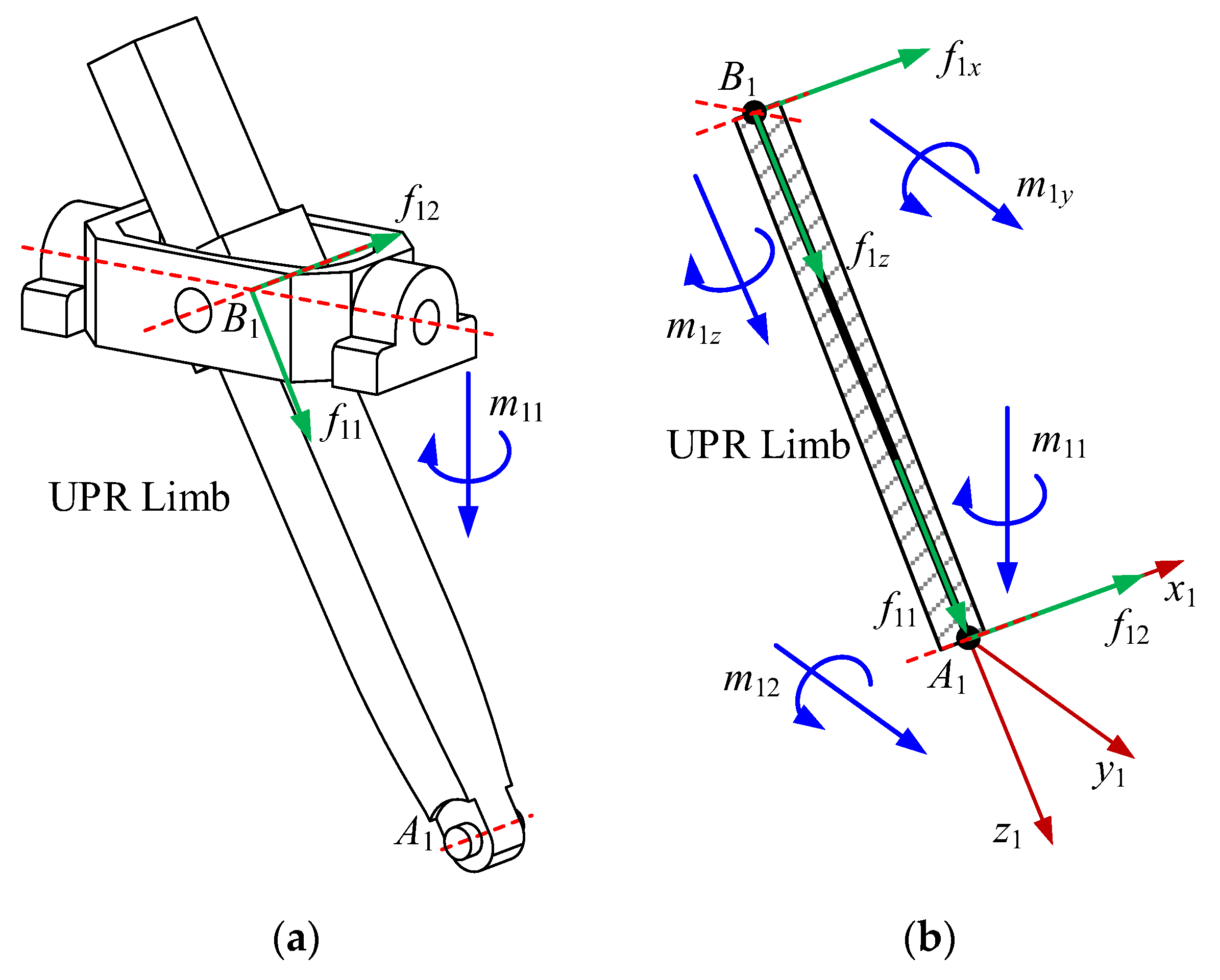
3.1. Stiffness Matrices of UPR Limbs
In this section, the wrenches including actuation and constraint are determined first. Based on the results in [
32] and the limb structure in
Figure 1 Reference source not found, one actuation wrench,
, and two constraint wrenches,
and
, of the first UPR limb can be deduced, where
represents the actuation force passing through the point
and along the
,
represents the constraint force passing through the point
and along the rotational axis of the R joint, and
represents the constraint couple perpendicular to the U joint. The magnitudes of these wrenches are defined as
,
, and
, respectively, as shown in
Figure 3a.
A limb coordinate frame
is established for the convenience of projecting these wrenches, as shown in
Figure 3b, where the
-axis points along the axis of the R joint, and the
-axis points along
. Furthermore, the force
acting at
can be equivalent to a force
acting at the point
and a couple
along the
-axis, and the
can be expressed as
As shown in
Figure 3b, the internal forces/torques at any cross-section of the first UPR kinematic limb can be written as
where
denotes the direction of the couple
, and
denotes the distance from the cross-section to the point
.
The strain energy of the first UPR limb can thus be expressed as
where
and
denote the elastic and shear modulus of limb 1, respectively.
denotes the area of the cross-section of limb 1, and
denotes the effective shear area of the cross-section along the
-axis.
denotes the area moment of inertia of the cross-section about the
-axis, and
denotes the polar moment of inertia of the cross-section.
Then, the deformations of this limb along the directions of these three wrenches,
, can be obtained as
The above results can be written in the matrix form of the relationship between the deformations and wrenches as
and
The stiffness matrix
of limb 1 can thus be written as the inverse of the compliance matrix
as
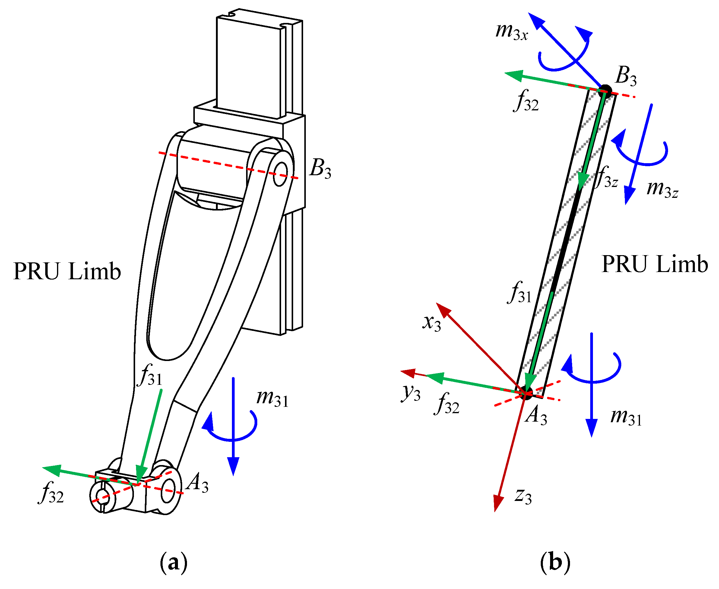
3.2. Stiffness Matrices of PRU Limbs
The process of calculating the stiffness matrix of the PRU limb is introduced below, which is similar to that of the UPR limb. For the PRU limb, one actuation wrench,
, and two constraint wrenches,
and
, also should be determined first. Based on the results in [
32],
represents the actuation force passing through the point
and along the
,
represents the constraint force passing through the point
and along the rotational axis of the R joint, and
represents the constraint couple perpendicular to the U joint. The magnitudes of these wrenches are defined as
,
, and
, respectively, as shown in
Figure 4a.
The decomposed results of three wrenches along the axes of the limb coordinate frame
are shown in
Figure 4b, in which the directions of
and
-axes are along the rotational axis of the R joint and
, respectively. The internal projection forces/torques at any cross-section of the PRU limb along the directions of local axes can be written as
where
denotes the direction of the couple
, and
denotes the distance between the cross-section and
.
The strain energy of the first PRU limb can thus be expressed as
where
and
denote the elastic and shear modulus of limb 3, respectively.
denotes the area of the cross-section of limb 3, and
denotes the effective shear area of the cross-section along the
-axis.
denotes the area moment of inertia of the cross-section about the
-axis, and
denotes the polar moment of inertia of the cross-section.
Similarly, the relationship between the deformations of the first PRU limb,
, and wrenches also can be written as
and
The stiffness matrix
of limb 3 can thus be written as
Through the above analysis, the strain energy of limbs can be obtained, followed by the stiffness matrices of the UPR limb and PRU limb. It should be noted that each link in the above study is assumed with a uniform cross-section, as explained in Equations (8) and (14). For other links with complicated structures, such as step links with different cross-sections and links with gradient cross-sections, the expressions of Equations (8) and (14) should be modified accordingly. At this time, the area, effective shear area, area moment of the inertia, and polar moment of inertia of the cross-section will not be constant, which will be the focus of our follow-up research.
3.3. Overall Stiffness Matrix of the 2UPR–2PRU PM
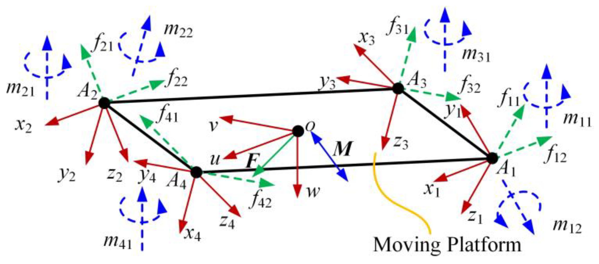
For the 2UPR–2PRU PM, the small configuration variations of the point in the moving platform can reflect the overall stiffness performance, which is determined by the reaction wrenches from the four limbs and external load
, as shown in
Figure 5. The external load
acts on the origin of the moving platform, in which
F and
M denote the vectors of applied external force and moment, respectively. First, the equilibrium equations that describe the reaction wrenches and external loads can be directly obtained as
where
,
,
, and
denote the wrench matrices of four limbs, respectively.
,
,
, and
denote the magnitude vectors of four limbs, respectively.
Then, the deformation of the origin of the moving platform
can be related to the deformations along the direction of wrenches in all limbs as
from which the relationship between
(
i = 1, 2, 3, and 4) and
can be expressed as
.
Based on the above results, the mapping between the external loads and deformation vector can be obtained as
from which the stiffness matrix
of the 2UPR–2PRU redundantly actuated PM can be written as
In summary, the analytical limb and overall stiffness models of the redundantly actuated 2UPR–2PRU PM have been developed, which have intuitive forms of expression and clear physical meanings. These theoretical results also can provide references for actual applications, such as the trajectory planning of prototypes.
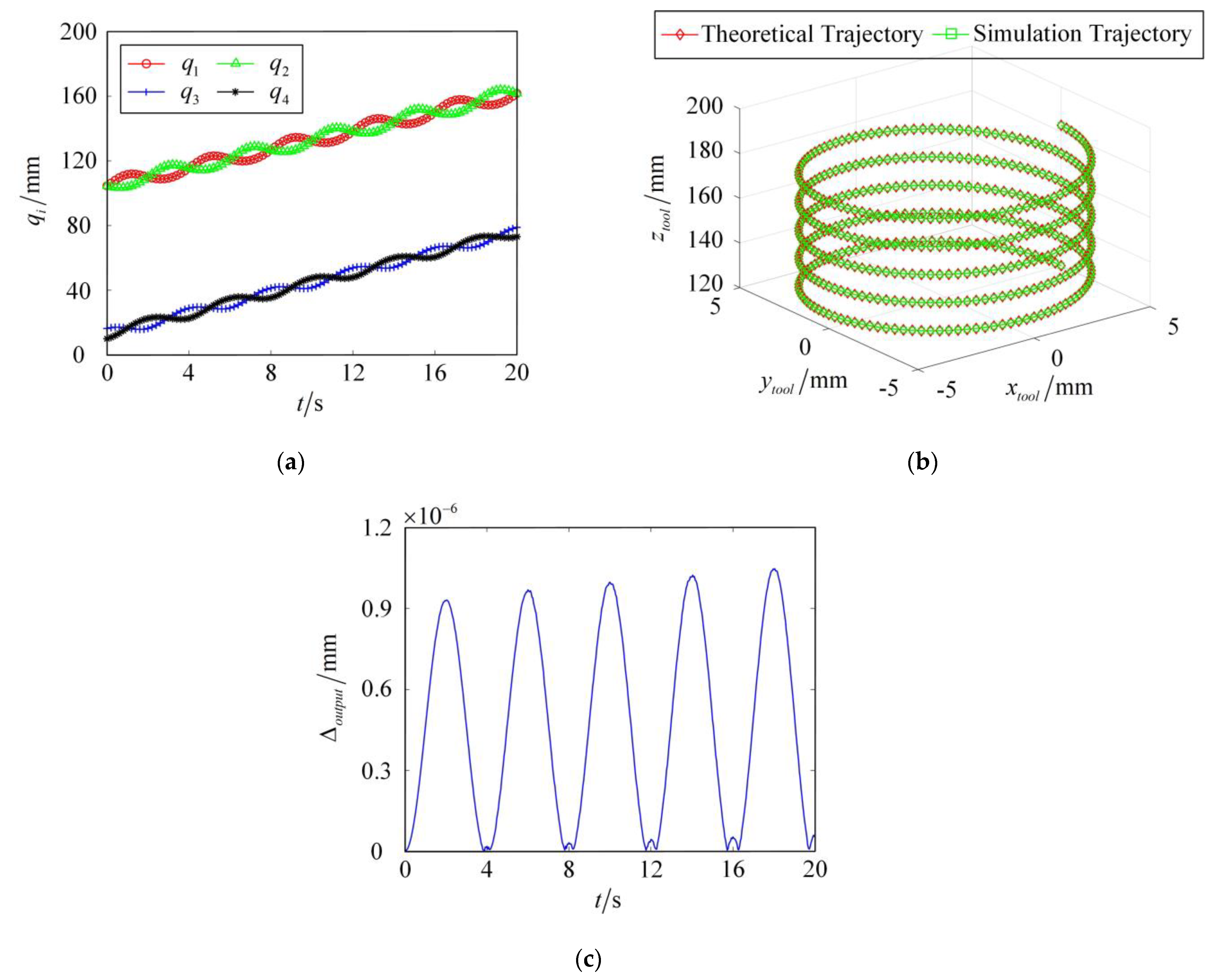
3.4. Comparisons of Theoretical Results with the FEA Method
In this section, the FEA method is used to verify the correctness of the theoretical stiffness model of the 2UPR–2PRU PM with actuation redundancy. Under the external load, the precise stiffness and deformation results of the PM can be provided by establishing the corresponding finite element model in ANSYS software. In the finite element model, the connections between the fixed base and the actuated joints are grounded, and the moving platform and all kinematic joints are set as rigid. To obtain the simulation results with high precision, the flexible links in the model are established by using the element beam188 based on the Timoshenko beam theory, which is a three-dimensional beam element with two nodes. Additionally, the beam element is set as quadratic. It considers the shear deformation effects during the simulation and can accurately express the spatial deformations of links. The link parameters, including the lengths and material characteristics of the redundantly actuated 2UPR–2PRU PM, are listed in
Table 1. In this paper, the cross-sections of four limbs are defined as the solid circular sections with the same size,
(
i = 1, 2, 3, and 4), and the elastic modulus and shear modulus of four limbs are the same in this investigation, namely,
and
(
i = 1, 2, 3, and 4). In addition, the Poisson’s ratio
is the same.
To demonstrate the correctness of theoretical results, four configurations of redundantly actuated 2UPR–2PRU PM with different external loads are chosen as verified cases in this study, as shown in
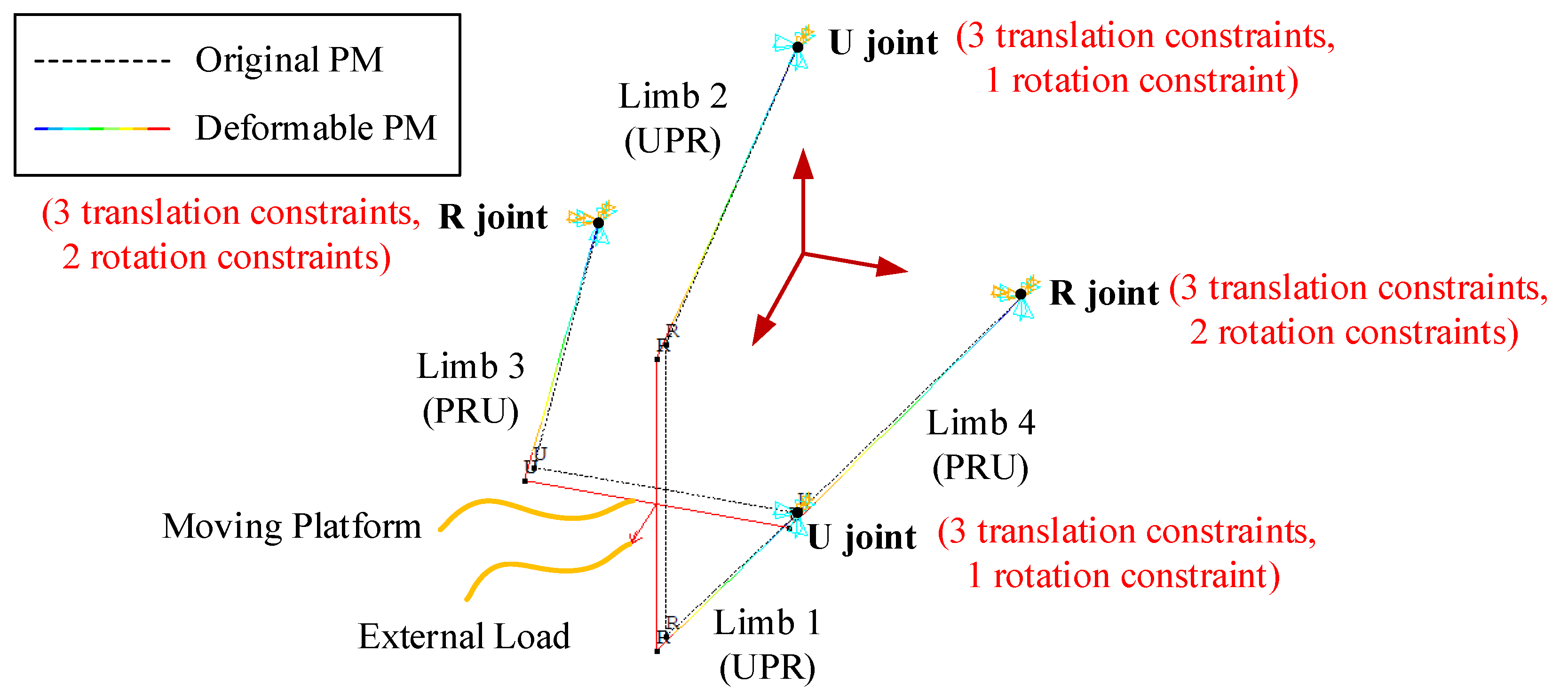
Table 2. The boundary conditions of the redundantly actuated 2UPR–2PRU PM exported by the ANSYS software are provided in
Figure 6, in which the PM in case 1 is taken as an example. The applied constraint situations and external load of the 2UPR–2PRU PM can be found, in which the U joint in the UPR limb is subjected to three translation constraints and one rotation constraint, and the R joint in the RPU limb is subjected to three translation constraints and two rotation constraints. Additionally, an external load is applied to the center point of the moving platform.
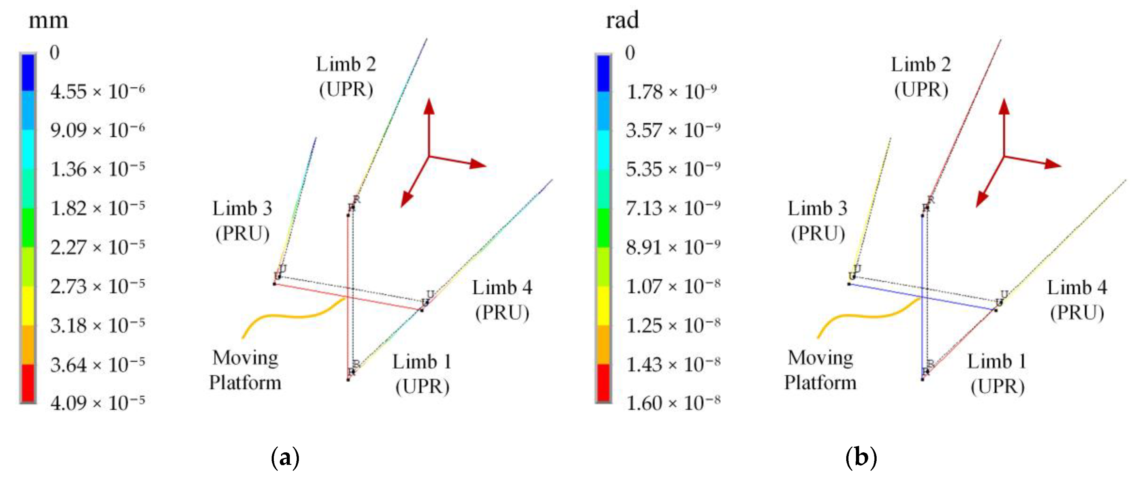
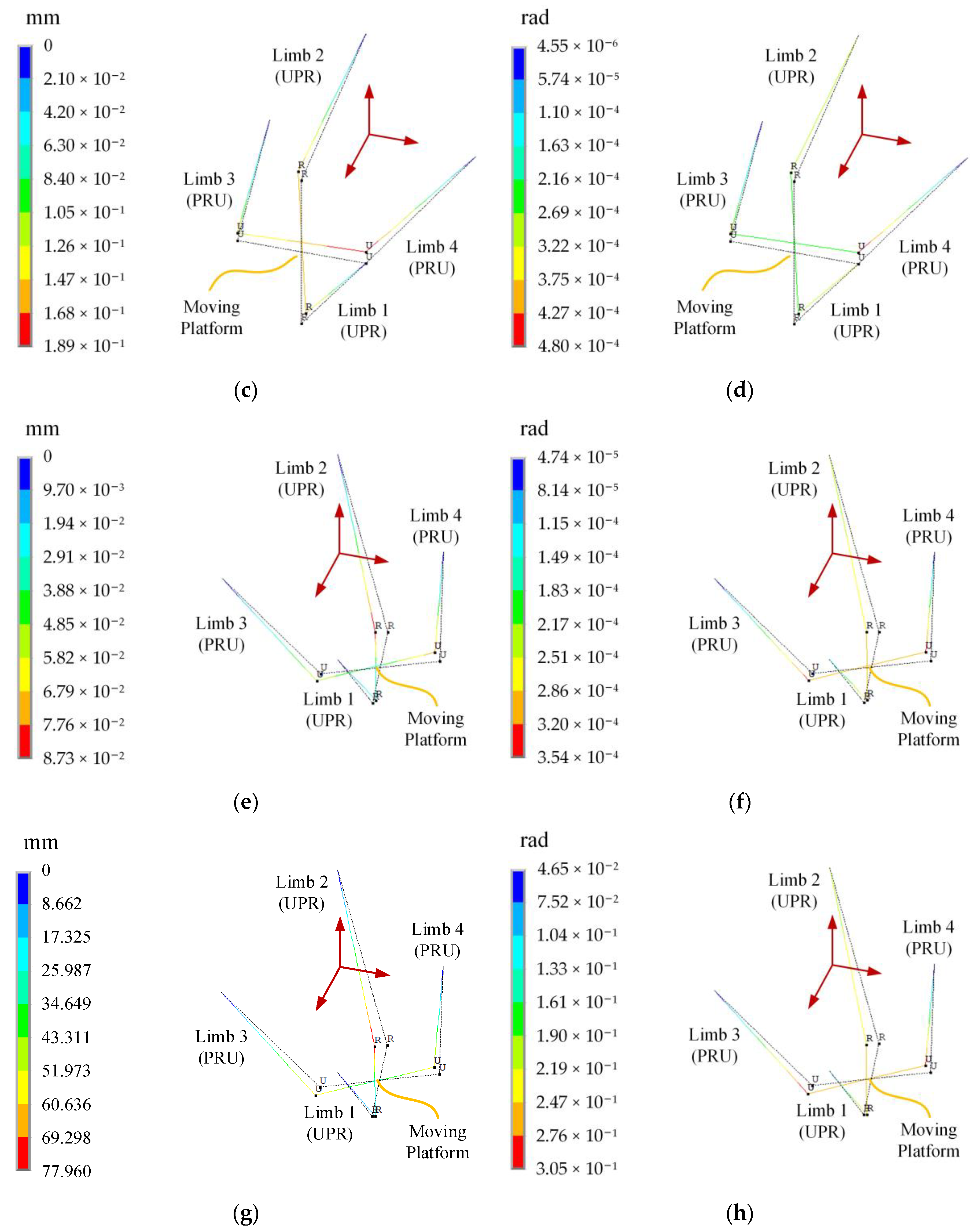
Figure 7a–h depicts the linear and angular deformations in the four cases in the software ANSYS, which can show the influence of different external loads on the 2UPR–2PRU PM to some extent. In
Figure 7a,b, the two rotating angles of the moving platform are zero, and it is only subjected to a simple external load along the
z-axis. Since the 2UPR–2PRU PM has a symmetrical structure in this case, the center of the moving platform only has a small linear deformation along the
z-axis, and there is no angular deformation. In cases 2 and 3, as shown in
Figure 7c–f, since the moving platform is subjected to a combined external load, the moving platform has small linear and angular deformations. The results in the above figures show that the deformation is related to the configuration and external load. In case 4, as shown in
Figure 7g,h, the moving platform is subjected to a huge external load, which leads to large linear and angular deformations.
Table 3 also lists the values of deformations of the center of the moving platform in four examples by using theoretical and FEA models. In the first three cases with small deformations, the results obtained from the theoretical and FEA models are almost the same, and all the relative errors of deformations in these cases are less than 0.67%, which is very low and can be acceptable. In the fourth case with large deformation, the maximum value of relative errors is only 3.52%, which proves that the theoretical model can also be used for the prediction of the case with large deformation. All the results show that the beam element used in the simulation is enough to validate the theoretical method. The developed theoretical model is universal, which makes it suitable not only for cases with small deformations but also for large deformation prediction. Therefore, the compliance/stiffness matrix of the 2UPR–2PRU PM with actuation redundancy obtained from the theoretical model can be regarded as an alternative to that obtained from the FEA model and also provide the foundation for the following stiffness performance evaluation.
4. Stiffness Performance Evaluation of the Redundantly Actuated 2UPR–2PRU PM
Since the dimensions of elements in the general stiffness matrix are different, some common stiffness indices, such as the maximum and minimum eigenvalues [
39] and average of the eigenvalues [
11], will lead to unclear physical meanings and erroneous interpretations [
40]. In addition, some stiffness indices can separate the translations and rotations [
39,
41,
42], such as the stiffness indices based on the linear stiffness and angular compliance ellipsoids [
39]. In this paper, the stiffness index proposed by Yan et al. [
34] is used to measure the elastostatic stiffness characteristics of the 2UPR–2PRU PM with actuation redundancy. This criterion evaluates the stiffness property of a PM based on the energy and related to the direction of external load. This index can intuitively measure the capability of the PM to resist the external load in a certain direction, and it is defined as
where
is the overall compliance matrix, and
denotes the virtual work of a PM under the external load. Through the multiplication combination of
and
, the dimension is unified into the joule (J), and after the inversion, the unit of the index changes into the inverse of the joule (J
−1). For example, 1 J
−1 means that the equivalent deformation of a PM is 1 mm when the external load is 1000 N. It is obvious that the bigger the value of
, the stiffer the configuration.
Using the link parameters listed in
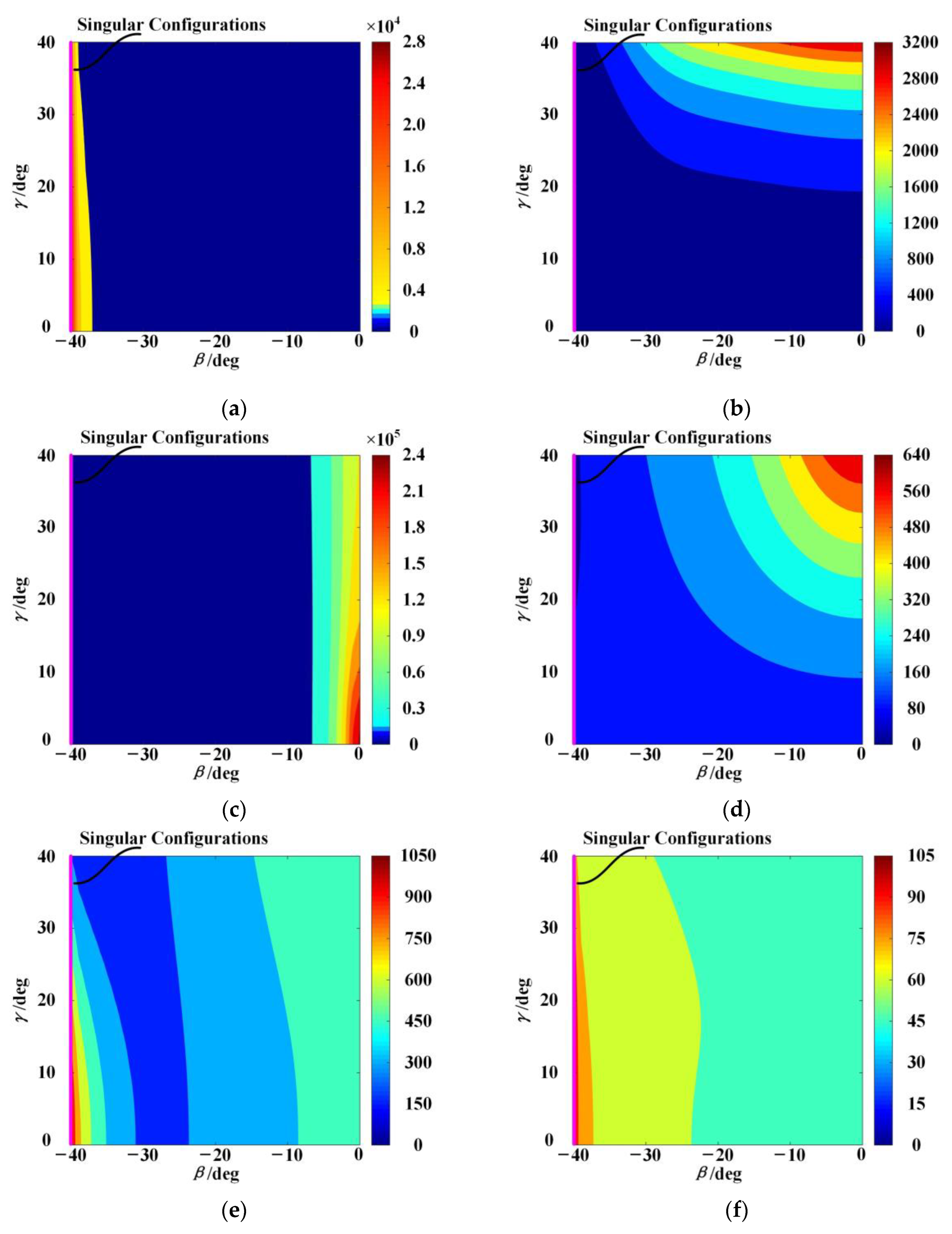
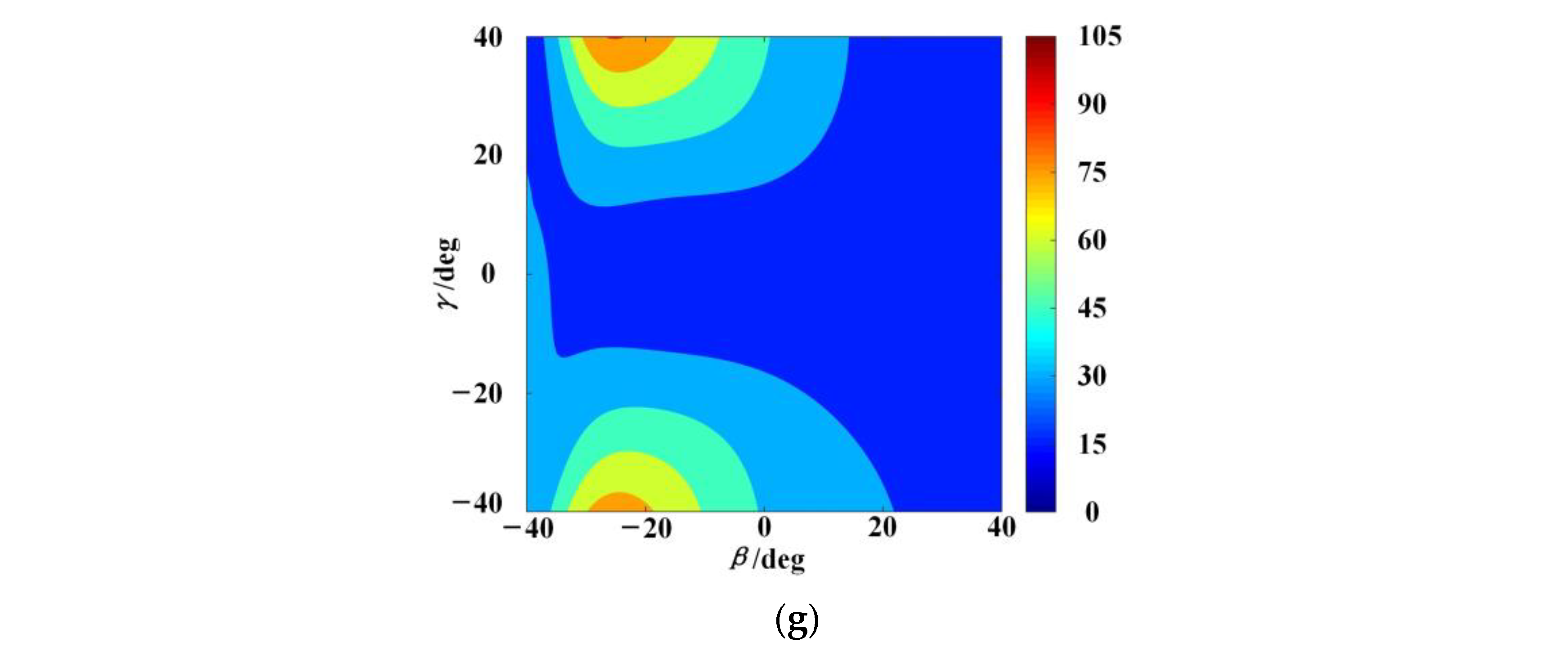
Table 1, the distributions of
under different single external loads are shown in
Figure 8a–f. All of them are limited in operational height
. Since all of them are symmetric about the plane
and
, only the top-left quarter of each distribution is depicted. The distributions of
under single external force and couple loads are completely different due to the structural characteristics of the 2UPR–2PRU PM. For the different external force loads, as shown in the results in
Figure 8a–c, the orientation ranges of the PM with better stiffness performance are different, and the 2UPR–2PRU PM with actuation redundancy has better resistance to the external force load along the
z-axis, which is determined by the structure arrangement. For the different external couple loads, as shown in
Figure 8d–f, the influence of the couple on the stiffness performance of the 2UPR–2PRU PM is different from that of the force, from which one can find that the 2UPR–2PRU PM has better resistance to the external couple load along the
y-axis. In addition, the distributions of
in a combined external load are shown in
Figure 8g, which are different from the results in
Figure 8a–f. This is caused by the influences of the external load on the overall stiffness of this PM.
The elastostatic stiffness performance above can also be related to the singularity of the PM. The stiffness performance of the PM in the singular configuration can be clearly described by using the above stiffness indices under single external loads. In [
32], it has been proved that the redundantly actuated 2UPR–2PRU PM is in the inverse kinematic singular configurations when the link
or
is parallel to the
x-axis. Using the link parameters and operational height above, the 2UPR–2PRU PM reaches the singular configurations when
or
, which have been highlighted in pink in the top-left quarter of each distribution, as shown in
Figure 8a–f. In
Figure 8a–c, the 2UPR–2PRU PM under the singular configurations has better stiffness performance when the single external force is along the
x-axis. However, the stiffness performance of the PM is poor when the single external force is along the
y- or
z-axis. In addition, the 2UPR–2PRU PM under the singular configurations has poor stiffness performance when a single external couple is applied on the moving platform, no matter in what direction, as shown in
Figure 8d–f. To summarize, the 2UPR–2PRU PM with redundancy actuation has relatively good resistance to a single external force along the
x-axis in singular configurations. Compared with the values of the stiffness index under the external force along the
x-axis, these values under other external forces or couples are so small and can be approximated as zero. It should be noted that although the stiffness model developed in this study is a simple one with some assumptions, the above results can provide references for avoiding singular configurations and selecting the suitable workspace.
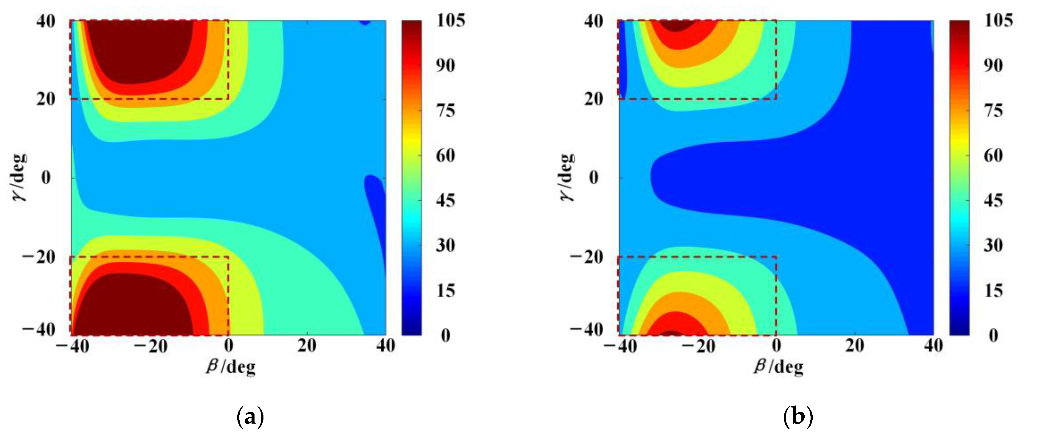
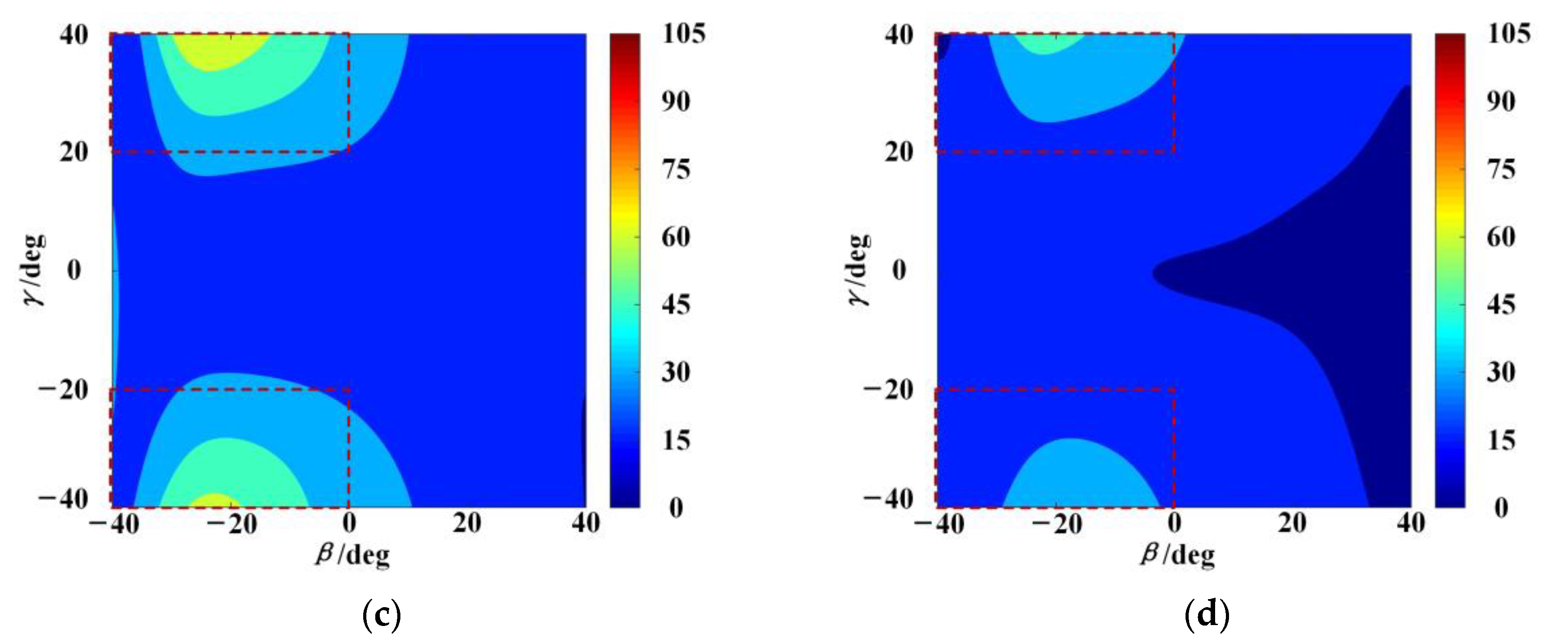
The distributions of
under a combined external load in the different operational heights are also discussed in this paper.
Figure 9a–d shows the distributions of
in the different operational heights when
. The stiffness performance becomes worse with the increase of the operational height. Under this external load, the redundantly actuated 2UPR–2PRU PM has a better stiffness performance in the orientation ranges where
and
, and
and
. To demonstrate the superiority of the mechanism stiffness in the selected orientation ranges, the minimum, maximum, and average values of the stiffness index in the above selected ranges and other ranges are listed, as shown in
Table 4. It can be seen that in the different operational heights, the minimum, maximum, and average values of the stiffness index in the above selected orientation ranges are larger than those in the other orientation ranges. The relative proportion ranges from 106.36% to 257.84%. From the results in
Figure 8 and
Figure 9, it can be concluded that the magnitude and direction of the external load have a major impact on the distributions of stiffness performance of the 2UPR–2PRU PM, which provides guidance for the selection of application scenarios and a suitable workspace. Furthermore, in some special application scenarios where an external load in a specific direction is required, the distributions of stiffness performance can also be used for structural design and trajectory planning [
34].
5. Conclusions
This paper establishes the elastostatic stiffness model of the redundantly actuated 2UPR–2PRU PM in the analytical form, including the limb stiffness models and overall stiffness model. Based on the principle of the strain energy, the expression of actuation and constraint wrenches, the strain energy in the limb, and the deformations along the direction of each wrench are successively derived in this paper, and then the analytical expressions of the stiffness matrices are obtained. All the results in the stiffness analysis have intuitive forms of expression and clear physical meanings, which can provide references for actual applications. Comparable results of numerical examples with ANSYS show that all the relative errors of the deformations in the three cases with small deformations are less than 0.67%, and all the relative errors of the deformations in the case with large deformations are less than 3.52%; these results verify the correctness and universality of the stiffness model of 2UPR–2PRU PM. The stiffness index based on energy is adopted to evaluate the stiffness performance under different external loads. Using this stiffness index, the performance in singular configurations can also be measured. In addition, this index can also provide good guidance for the selection of workspaces with better performance. Based on the above foundation, our future work will focus on the extension of the stiffness model, such as the establishment of a complete stiffness model that takes the compliance of joints, links, and the end-effector and the influence of frictional effect into account. The links in the limbs will not be assumed with a uniform cross-section. The area, effective shear area, area moment of the inertia, and polar moment of the inertia of the cross-section will not be constant. Error modeling, trajectory planning, and control will also be focused on in the future.


