Optimization of Gain Scheduled Controller for an Active Trailer Steering System Using an Evolutionary Algorithm

Abstract

Car–trailer combinations can experience unstable motion modes such as trailer-sway, jackknifing and rollover that can lead to fatal accidents. These unstable motions can be mitigated with the use of an active trailer steering (ATS) system. Prior studies in ATS have leveraged the linear quadratic regulator (LQR) as an ATS controller but for many of these designs it was assumed that the vehicle and operating parameters were constant. In reality, vehicle and operating parameters may vary and have an impact on the stability of a car–trailer combination. In this paper, the weighting matrices of the LQR controller are determined using the GDE3 evolutionary optimization algorithm with the objective of addressing the design trade off between minimizing the car–trailer’s path-following performance for low vehicle speeds and minimizing the rearward amplification for high vehicle speeds. The effectiveness of the approach is demonstrated using a numerical simulation car–trailer model developed in the CarSim simulator. Our results show that the multi-objective tuned gain scheduling controller outperforms a non-tuned gain scheduling controller in terms of improving the lateral stability and the path following performance of car–trailer combinations in driver in the loop single lane-change maneuvers at a constant vehicle forward speed.

1. Introduction

A typical car–trailer system consists of a leading vehicle unit, supplying the power to the combination, and a trailing unit, connected with a mechanical hitch. The hitch connection between the vehicle units generates several mechanical constraints, making the dynamics and kinematics of this combination more complex to investigate compared to a single-unit vehicle, e.g., car or truck. Due to the unique dynamics of the combination and the mechanical constraints, the car–trailer system usually experiences unstable motion modes that could lead to fatal accidents. Typical unstable motion modes that lead to crash of car–trailer combinations are trailer-sway, jackknifing and rollover [1]. Several factors can lead to each of the aforementioned unstable motion modes, e.g., high-speed evasive maneuvers, crosswinds, road conditions and payload variation of the trailer [2].

The detrimental effect of the three aforementioned unstable motion modes is reduced by using various vehicle safety design strategies. These strategies can be passive and active. Passive strategies require no additional energy or complicated implementation whereas active strategies do require additional energy to provide active safety actuations. The strategy considered in this research is an active trailer steering (ATS) system. This system requires a steering actuator to steer the wheels of the trailer of a car–trailer combination.

Command trailer steering systems allows car–trailer combinations to operate on a fix steer ratio between the tractor steering angle in relation to the trailer axle steering angle [3]. Using an ATS, one can work with conflicting objectives using an actively optimized controller. This improves Rearward Amplification (RWA) at high speeds and Path-Following Off-Tracking (PFOT) at low speeds, without having to use multiple modes of operation and worrying about switching between them. ATS technology is just a name for many ways to control the trailer steering system. Generally, ATS systems can be tuned to enhance stability at high speeds but these speeds can vary across different highways. ATS requires optimization for independent operation and one of the control algorithms used in ATS is the Linear Quadratic Regulator (LQR) [4]. LQR though is a linear controller and for many of these designs it was assumed that the vehicle and operating parameters were constant. In reality, vehicle and operating parameters may vary and have an impact on the stability of a car–trailer combination. For example, varied vehicle forward speeds and trailer payloads may impose negative impacts on the directional performance of the car–trailer combination such that the LQR-based ATS controller operates beyond the limits that it was optimized for and may result in an unstable car–trailer behavior.

To address this problem, an LQR-based ATS controller with a look-up table gain-scheduler is proposed which is used to stabilize a car–trailer combination at different vehicle speeds. The goal of the gain scheduler is to choose the appropriate LQR gains for the ATS controller depending on the design trade off between PFOT and RWA. The weighting matrices of the LQR controller in the scheduler are determined using an evolutionary optimization algorithm, namely GDE3 [5]. The dual optimization approach, using GDE3 and LQR, is proposed because one cannot easily specify the continuous objective function for the global optimization problem. Our approach is a two layer optimization problem where LQR is used to stabilize the car–trailer combination at specific speeds and GDE3 is used to optimize the car–trailer combination for different speeds.

The effectiveness of the proposed two layer optimization method for ATS controller design is demonstrated using numerical simulation based on a car–trailer model developed in the CarSim simulator. To the best of our knowledge, Generalized Differential Evolution (GDE) has not been previously used to tune an LQR controller for any control system let alone for ATS control.

In Section 2, we present some prior work in the use of evolutionary algorithms for the optimization of controllers as well as a brief review on the optimization of controllers for ATS in car–trailer and truck–trailer combinations. Section 3 presents a background into car–trailer stability metrics as well the GDE algorithm. Section 4 introduces the proposed two-layer optimization method for determining the control gain matrix under a given driver reaction time and a vehicle forward speed. Section 5 presents the design of a gain Scheduler for an ATS-enabled car–trailer combination. Section 6 presents several simulation results for PFOT and RWA of an ATS-enabled car–trailer combination using the optimized GDE controller gains for different vehicle speeds and driver reaction times. Finally we conclude and present some limitations to our approach in Section 7.

2. Literature Review

Evolutionary algorithms (EAs) and multi-objective evolutionary algorithms (MOEAs) are proven to be effective in offline tuning of control systems for various applications [6]. The authors in [7] studied the effectiveness genetic algorithm (GA) in tuning of PI and LQR controllers for boiler-turbine plant.

The authors in [8] used a non-dominated sorting genetic algorithm (NSGA-II) as a MOEA to optimize an Heating, Ventilating and Air-Conditioning (HVAC) control systems. NSGA- II achieves an improvement, within the design constraints, while considering multiple objectives.

EAs were employed to optimize an LQR controller [9,10]. The authors of [10] concluded that differential evolution, along with other continuous optimizers, outperforms genetic algorithms, which reinforces the selection of Differential Evolution as the core optimization method.

An ATS control system, using the LQR-based controller, for articulated vehicles was designed and optimized by GA in [4] and shows that it is superior to other prior work. A GA optimized active trailer differential braking system is outlined in [11] for a car–trailer combination. The aforementioned studies along with engineering applications show that evolutionary search algorithms are ideal for tuning control systems in a wide array of applications [6].

Research in our paper combines two areas: utilizing the LQR technique for ATS controller design and using evolutionary algorithms to optimize the LQR control parameters. The LQR technique has been utilized to design the ATS controller for an articulated heavy vehicle (AHV) [12]. The study used a genetic algorithm to optimize the LQR controller for the ATS of AHVs, and demonstrated the strength of the LQR controller, and also elaborated on the importance of optimization. The work in [13] uses an LQR controller to control an anti-roll bar, which prevents vehicle rollover and they demonstrate how the LQR controller can provide stability to vehicular systems.

All the above studies, collectively, show that the LQR control method is used for various systems and that evolutionary algorithms achieve a better solution than other conventional methods or even fuzzy logic controllers. The difference in our approach over other approaches is the use of MOEA and GDE3 for tuning and creating a gain scheduler for an ATS-enabled car–trailer combination. GDE3 has also been proven to be better than the counterpart genetic algorithms [14,15].

3. Background

3.1. Car-Trailer Stability Criteria

For all Articulated Vehicles (AV) there are two major modes of operations: (1) high-speed evasive maneuvering and (2) low-speed path-following. When the AV is traveling at high speeds, it requires to be laterally stable. Without lateral stability roll-over can occur. The lateral stability of an AV is measured using the RWA [16] criterion. At low-speeds the trailer must follow the same trajectory as the car. If the trailer is unable to follow the same path as the car, this will result in a swept path, and a wider road is required for the safe operation of the car–trailer combination. The measure to check the trailer’s ability to track the path of the car is called PFOT [4,17] criteria.

An AV’s RWA is evaluated using a single-lane change maneuver at high speeds. During this maneuver the ratio of the lateral acceleration observed at the center of gravity (CG) of the trailer and the car [18] is measured. An ideal RWA is 1, which is extremely difficult to achieve in real-world operating conditions. Physically, when the RWA takes the value of 1.0, the trailing vehicle unit will have similar dynamic behaviors as the leading vehicle unit. In other words, with the RWA measure of 1.0, the AV will have better path-following capability, and the driver may well control the vehicle to achieve high lateral stability [18]. Controlling lateral acceleration amplification and achieving the RWA measure of 1.0 is the primary objective and Equation (1) is used to calculate the RWA ratio:

$$RWA=\frac{\left|PeaklateralaccelerationofthetraileratCG\right|}{\left|PeaklateralaccelerationofthecaratCG\right|}$$

(1)

PFOT is defined as the maximum radial offset between the path of the center of the car front axle and that of the center of the trailer rear axle over an evasive maneuver. Accurate measurement of PFOT can be performed by comparing the difference between the trajectory of the center of the car front axle and that of the center of the trailer rear axle during a circular motion of a car–trailer combination.

If an ATS controller is optimized for high-speed RWA, PFOT performance at low speeds will be hampered and vice versa [19]. This then results in an ATS controller that is optimized either for high-speed lateral stability or low-speed maneuverability. To conduct the RWA analysis, an open-loop testing procedure with a single lane change (SLC) maneuver is simulated. A single-cycle sine-wave steering input with adjustable frequency and amplitude represents the input for the SLC testing maneuver [20].

3.2. GDE3 Algorithm

In this work, we leverage the GDE3 evolutionary algorithm to compute the optimal weights of an LQR controller that controls the steering angle of the trailer.

GDE3 is a type of Differential Evolution (DE) [21] algorithm. Like all DE algorithms, GDE3 is a population-based metaheuristic (P-metaheuristic) evolutionary algorithm which has been inspired by Genetic Algorithms (GA). DE consists of mutation, crossover and selection, which performs best for continuous-valued problems.

The working principle of DE is similar to that used in for GAs. It starts with population initialization. During initialization all members are assigned fitness values according to fitness functions, these values correspond to how good these population members are for solving the problem.

Following initialization, the selection is made at random from the population space, anywhere between two and four members are chosen, depending on the utilized mutation scheme. There are more than ten mutation variants in DE [22] and we use the DE5 mutation scheme shown in Equation (2), where V is the mutant vector, F is the scaling factor with a value between 0 and 1, and $X_i$ are randomly selected individuals from the population.

$$V=X_{best}+F\ast (X_1-X_2)$$

(2)

The fitness of the population member, once chosen, is evaluated after it undergoes mutation and recombination. After applying the crossover and calculating the resulted offspring’s fitness value, the best parent and offspring is selected to the next generation (in GDE3 the selection follows a greedy strategy.).

The crossover or recombination method is as follows, regardless of the mutation method.

$$U\left(j\right)=\begin{array}{cc}V\left(j\right),\hfill & ifrand(0,1)<Cr\hfill \\ X_i\left(j\right),\hfill & otherwise\hfill \end{array}$$

(3)

where $U\left(j\right)$ is the population member created after recombination for a random value of j.

The DE parameters that are used in this paper are listed in

Table 1. Control parameters of optimization.

Parameter	Value
Population Size (P)	60
Crossover Probability ($C_r$)	$0.95$
Scaling Factor (F)	$0.3<F<0.9$
Number of Objectives	2

. These parameters are obtained from [22], in which the authors performed rigorous testing to show that these values produce optimal performance results.

4. Proposed 2-Layer Design Optimization Method

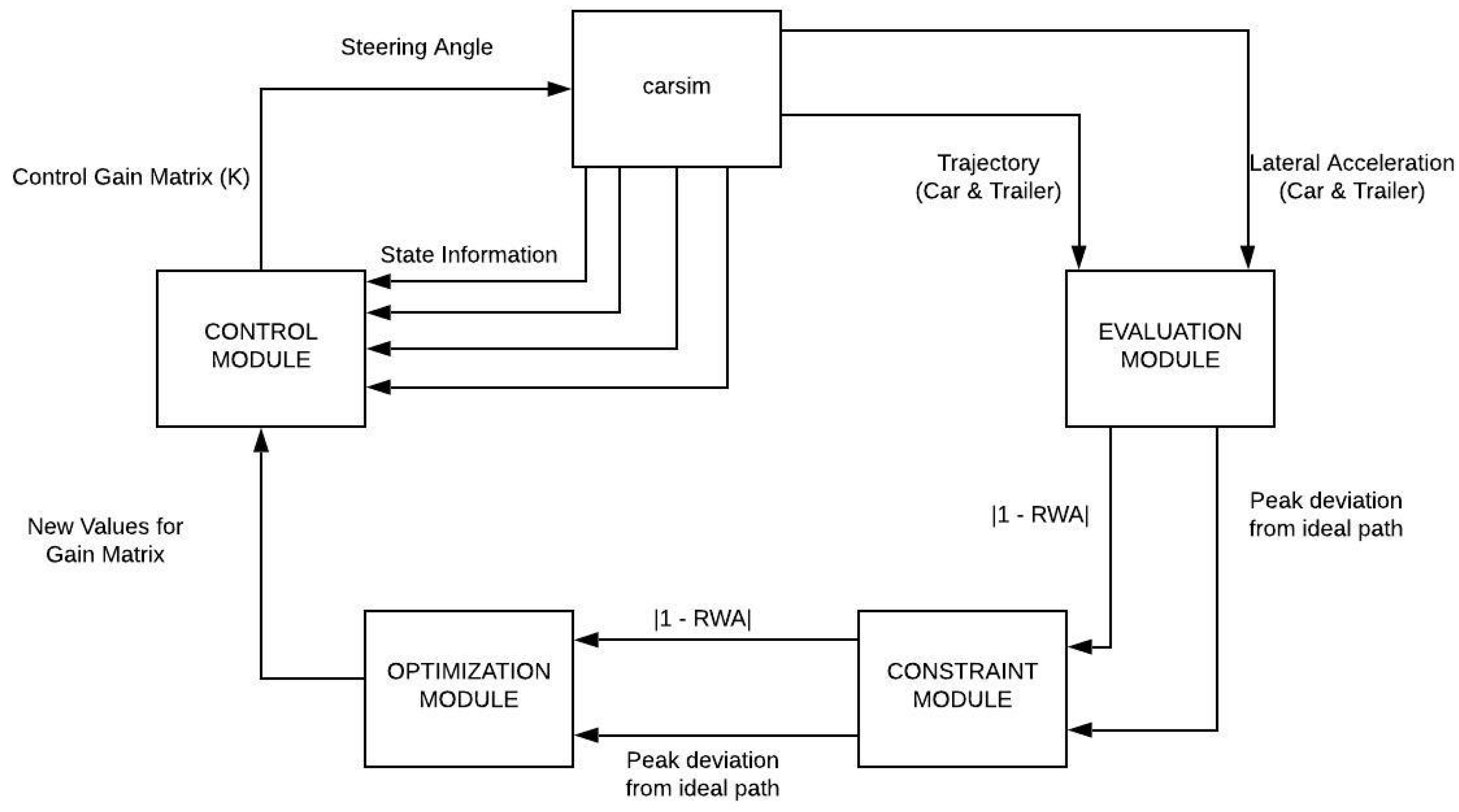
This research proposes a 2-layer optimization method for determining the LQR-based gain scheduling controllers (GSCs) for car–trailer combinations with active trailer steering. Figure 1 shows the framework of the 2-layer optimization method. At the upper layer is an optimizer, e.g., GDE3, while at the lower layer are the dynamically coupled vehicle system, including a virtual car–trailer plant; e.g., CarSim car–trailer model; virtual driver, such as CarSim built-in driver model; and an LQR-based controller.

With the given constraints and optimization variables $X_D$ from the upper layer, the vehicle and operating parameters of the vehicle system at the lower layer are updated. The operating parameters (or operating uncertainties) may include vehicle forward speed (U), trailer payload, road conditions, etc. Considering different drivers with various driving skills and habits, the parameters characterizing human drivers’ driving behaviors, such as, reaction time (t) and preview time, may be treated as a subset of the overall parameter set of the vehicle system [23,24]. Under varied operating conditions and considering different drivers with various driving skills and habits, the LQR controller’s gain matrix may be adaptively adjusted [25]. It is well known that with a given linear system, the control gain matrix of the LQR controller is directly determined by two weighting matrixes, i.e., Q (state variables associated) and R (control variables associated), and the performance index can be cast as,

$$J={\int }_0^{\infty }(x^{T}Qx+u^{T}Ru)dt$$

(4)

where x denotes state variable vector, and u control input vector. In the case concerned, Q and R are diagonal matrices. For the purpose of simplicity, it is assumed that Q and R are the corresponding vectors consisting the respective diagonal elements of each matrix. It should be mentioned that the LQR algorithm itself is an optimization technique for determining an optimal control gain matrix for the linear dynamic system. Thus, the optimization problem shown in Figure 1 is a 2-layer optimization problem. Thus, in this study, we set the design variable set as $X_D={\left[Ut{Q}^T{R}^T\right]}^T$.

Given a design variable set $X_D$, under a specified vehicle operating maneuver (e.g., single lane-change maneuver), the LQR algorithm will update its Q and R weighting matrices and derive the resulting control gain matrix K. At the lower layer of the 2-layer optimization problem shown in Figure 1, under the given operating maneuver, the virtual driver adaptively controls the front wheel steering angle ($\delta$) of the leading vehicle unit considering the vehicle state variable vector x; the LQR controller controls the trailer wheel steering angle (${\delta }_{A}TS$) in response to the driver steering angle ($\delta$) and the current vehicle state variable vector x; under the control of the virtual driver and the LQR controller, the virtual car–trailer plant executes the operating maneuver following the predefined path (e.g., single lane-change path) and forward speed scheme. Upon the completion of the operating maneuver, the directional performance measures, i.e., RWA($X_D$) and PFOT($X_D$), can be derived using the dynamic responses of the car–trailer plant over the operating maneuver. Then, the derived performance measures and associated dynamic responses over the operating maneuver will be sent back to the upper layer to evaluate the satisfaction of the constraints, i.e., $h\left(X_d\right)\le 0$ and $g\left(X_D\right)=0$, and to formulate and assess the fitness function formulated by

$$\underset{X_D}{min}F\left(X_D\right)=w_1·\left|(1-RWA\left(X_D\right))\right|+w_2·\left|PFOT\left(X_D\right)\right|$$

(5)

where $w_1$ and $w_2$ are weighting factors. It should be noted that both of the performance measures of RWA and PFOT are functions of design variable vector $X_D$. Within the defined design space, the optimizer, i.e., GDE3, at the upper layer of the optimization problem (as shown in Figure 1 will find the global optimal solution $X(D_{o}ptimal)$, which provides an optimal compromised solution between the performance measures of RWA($X(D_{O}ptimal$)) and PFOT($X(D_{O}ptimal)$).

For multi-objective optimization, with conflicting objectives, there is no single solution rather a set of solutions. Each solution consists of costs equal to the number of objectives. One solution is said to strongly dominate another solution if and only if all the costs of one solution are better than the other or if and only if all costs are no worse, and at least one is better. If a solution is not strongly dominated by any other solution then it is a Pareto solution [26]. An optimal Pareto-front is the set of all such solutions, which are not dominated by other solutions [27].

5. Design of a Gain Scheduling Controller for an ATS-Enabled Car-Trailer Combination

The method used to develop this gain scheduler is to generate a two-dimensional lookup table, using the driver model reaction time and vehicle forward speed to schedule an optimum set of gains for the LQR controller of the ATS-enabled car–trailer combination. CarSim [28] is a mechanical simulation tool and is used to simulate multi-body vehicle systems and analyze their dynamic behaviors. It is a useful tool for the analysis and design of active vehicle safety systems. In this section, CarSim acts as Software-in-Loop (SIL) and provides vehicle dynamic responses required to tune the controller.

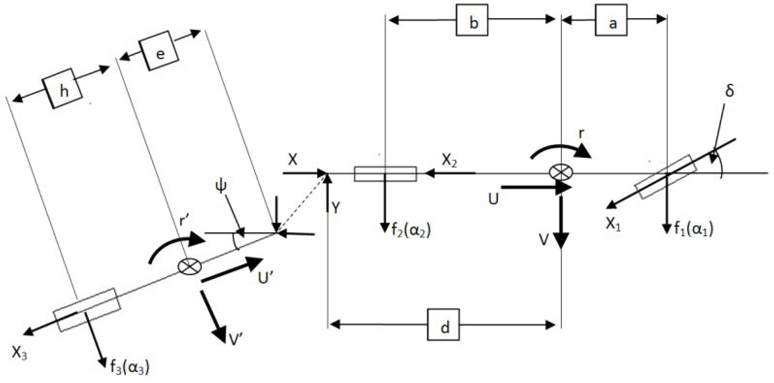
5.1. 3-DOF Linear Yaw-Plane Car-Trailer Model

The LQR controller tuned for this optimization is designed using a 3-DOF yaw-plane car–trailer combination model. The mathematical model has been derived and validated against other published models [29,30].

In this model, each axle is represented by a single wheel, assuming that both tires on each axle have the same dynamic characteristic, i.e., the relationship between the tire slip angle and the cornering force. Figure 2 shows the schematic representation of the car–trailer combination using the 3 DOF yaw-plane model.

For the yaw-plane model, the lateral and yaw motions of the car, as well as, the yaw motion of the trailer are considered. The governing equations of motion of the car are expressed as:

$$m_1(\dot{U}-Vr)=-X_{1}cos\delta -X_2+X$$

(6)

$$m1(\dot{V}+Ur)=f_1\left({\alpha }_1\right)+f_2\left({\alpha }_2\right)+X_{1}sin\delta -Y$$

(7)

$$I_1\dot{r}=a{f}_1\left({\alpha }_1\right)-b{f}_2\left({\alpha }_2\right)+\alpha X_{1}sin\delta +dY$$

(8)

where Equations (6)–(8) govern the longitudinal, lateral and yaw motions of the car, respectively, $m_1$ is the mass of the car, U forward speed of the car, V lateral speed of the car and r yaw rate of the car, $\delta$ is the front wheel steering angle, $X_i$ are the longitudinal tire forces, ${\alpha }_i$ are the slip angles of the tires, $f_i$ are the cornering stiffness of the tires, X is the longitudinal hitch force, Y is the lateral hitch force, $I_1$ is the moment of inertia of car and a, b, c and d are described in

Table 2. Car–trailer combination parameters for ATS controller design.

Description	Symbol
Car Mass	$m_1$
Car yaw inertia	$I_1$
Trailer mass	$m_2$
Trailer yaw inertia	$I_2$
Distance between car CG and its front axle	a
Distance between car CG and its rear axle	b
Distance between car CG and hitch point	d
Distance between trailer CG and hitch point	e
Distance between trailer CG and its axle	h
Height of car CG	$H{1}_{CG}$
Height of trailer CG	$H{2}_{CG}$
Combined car front tires cornering stiffness coefficient	$c_1$
Combined car rear tires cornering stiffness coefficient	$c_2$
Combined trailer tires cornering stiffness coefficient	$c_3$

.

Similarly, the governing equations of motion for the trailer are shown as follows:

$$m_2({\dot{U}}^{{}^{\prime }}-V^{{}^{\prime }}{r}^{{}^{\prime }})=-X_3-Ysin\psi -Xcos\psi$$

(9)

$$m_2({\dot{V}}^{{}^{\prime }}+U^{{}^{\prime }}{r}^{{}^{\prime }})=f_3\left({\alpha }_3\right)+Ycos\psi -Xsin\psi$$

(10)

$$I_2{\dot{r}}^{{}^{\prime }}=-h{f}_3\left({\alpha }_3\right)-e(-Ycos\psi +Xsin\psi )$$

(11)

where Equations (9)–(11) govern the longitudinal, lateral and yaw motions of the trailer, respectively, $m_2$ is the mass of the trailer, $U^{{}^{\prime }}$ forward speed of the trailer, $V^{{}^{\prime }}$ lateral speed of the trailer, $r^{{}^{\prime }}$ is the yaw angle of the trailer, $I_2$ is the moment of inertia of the trailer and h and e are described in Table 2.

Once a mechanical hitch is introduced, the kinematic constraint is active. To simplify the model, the forward speed of the car is assumed constant. In addition, the articulation angle, $\psi$ assumed to be small, which leads to Equations (12)–(14). Detail is available in [31].

$$cos\left(\psi \right)\approx 1$$

(12)

$$sin\left(\psi \right)\approx \psi$$

(13)

Furthermore, the following equation is determined at zero initial conditions.

$${\psi }^{{}^{\prime }}=r-r^{{}^{\prime }}$$

(14)

where $\psi$ is the articulation angle, r is the yaw rate of car and $r^{{}^{\prime }}$ is the yaw rate of the trailer. The notation is shown in Figure 2.

Once the model is derived, a multibody dynamic software package, known as Equation of Motion (EOM) is used to validate the model by comparing the responses of both models under the same single lane-change maneuver [32]. Both models generate the identical dynamic response, which proves that the EOM model matches the derived equations. Thus, the EOM software package is selected to design the ATS controller. However, in order to further enhance the model, more essential components are added to the system, e.g., an actuator is installed on the trailers axle, and an accelerometer is installed at the Centers of Gravity (CG) of the leading and trailing units, respectively. The actuator is used to produce torque to steer the wheels on the trailer axle. In addition, the trailer forward speed should be the same as the car forward speed as the assumption made previously.

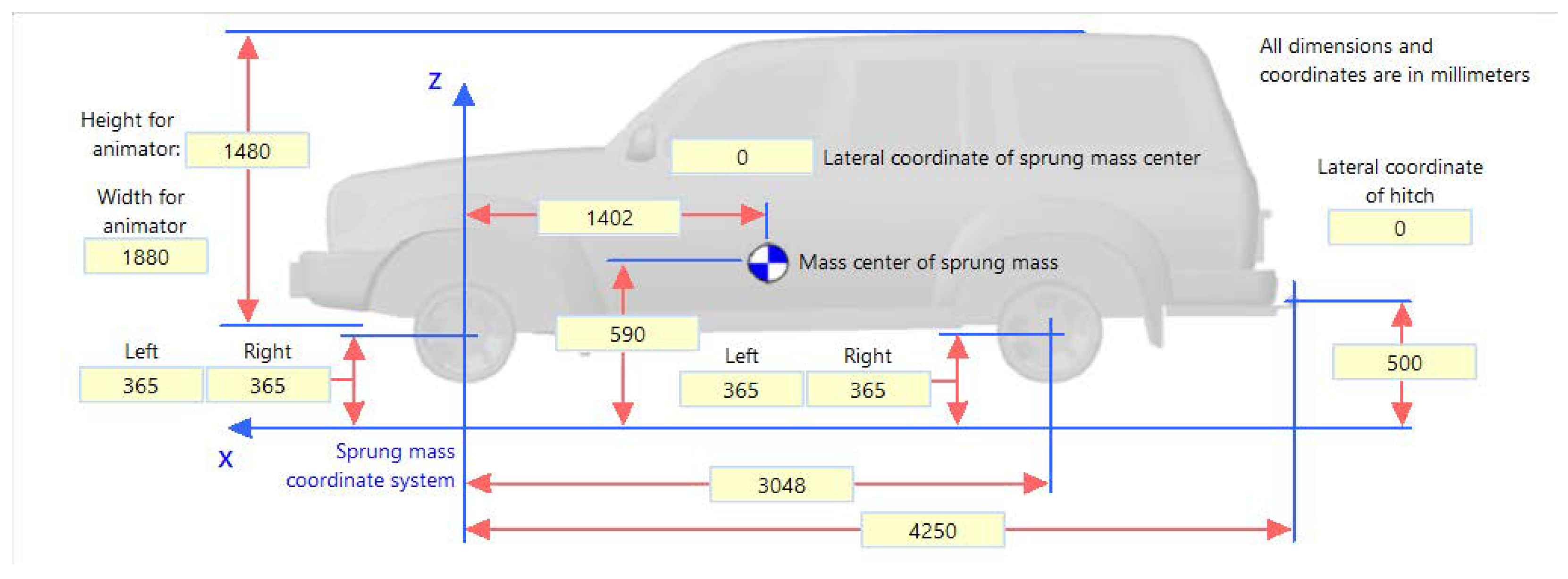
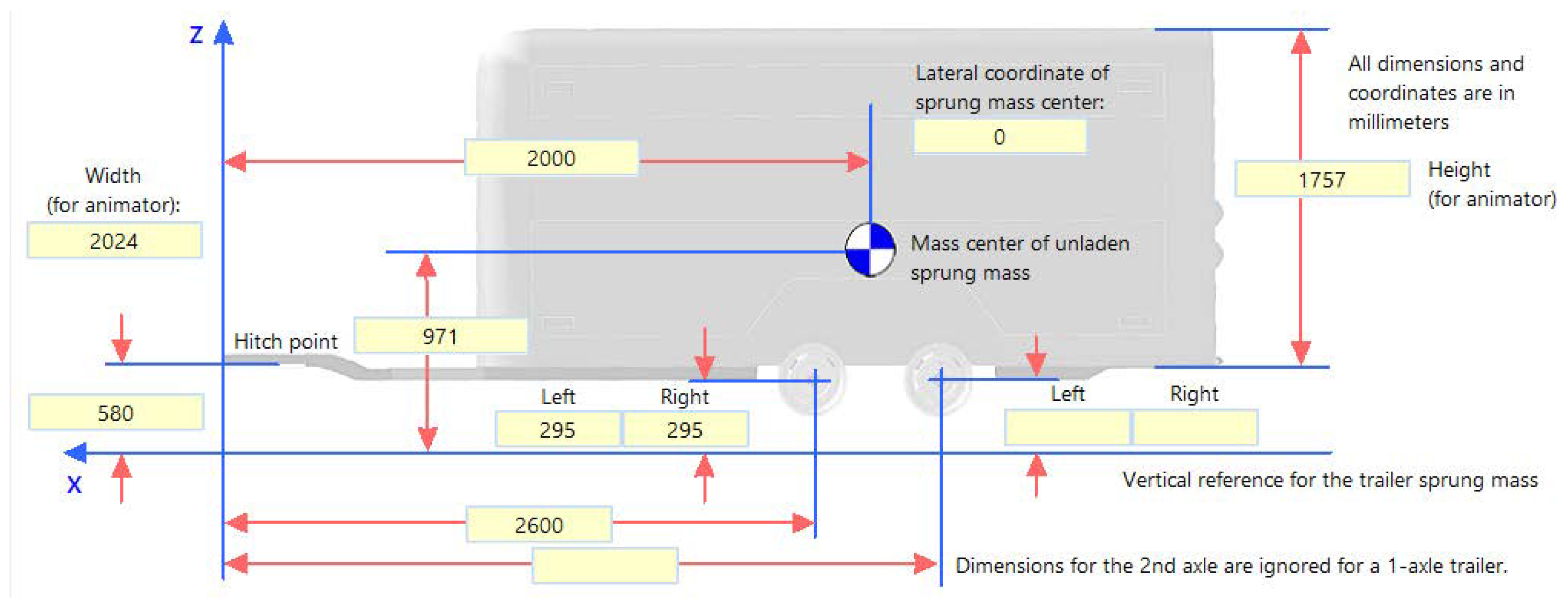
5.2. The CarSim Car–Trailer Model

In this research, a car–trailer combination with a full-size car and a single axle trailer is modeled using CarSim software. The parameters of the model are close with those of the car–trailer model reported in [30], which has been validated using numerical simulations.

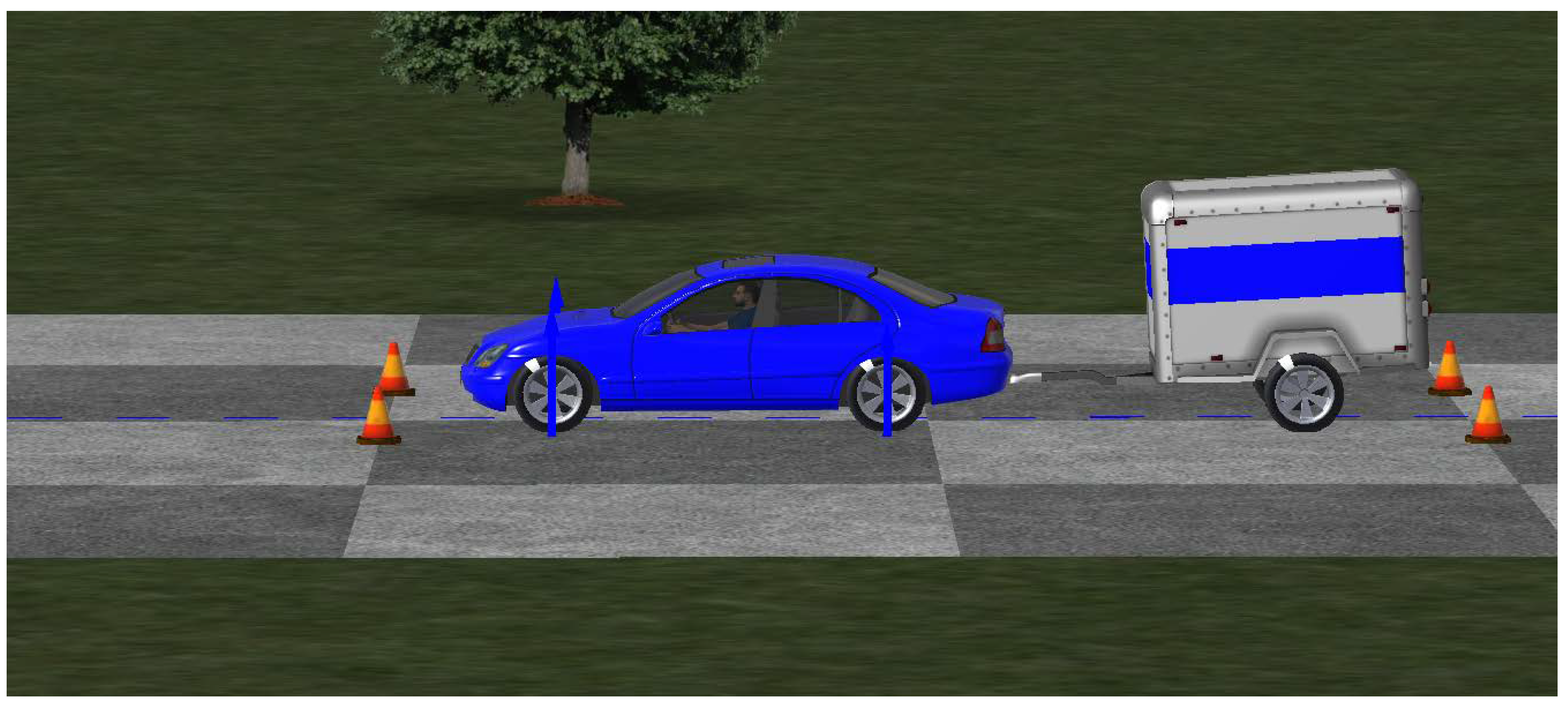
The car–trailer model for the co-simulation is directly developed and tested in CarSim software. Figure 3 and Figure 4 show the details of the car and trailer sub-models used in the co-simulation and Figure 5 is an image of the car–trailer model from CarSim created using these parameters.

In order to complete the CarSim vehicle model one requires the car and trailer mass and moments of inertia as listed in

Table 3. Vehicle parameter values.

Parameters	Value
mass of car	1653 kg
roll inertia of car	2765 kgm${}^2$
mass of trailer	466 kg
roll inertia of trailer	1810 kgm${}^2$

.

The co-simulation with CarSim model only requires the LQR control gain matrix, K that is generated directly using the GDE3 multi-objective evolutionary algorithm.

5.3. Built-in Driver Model in CarSim

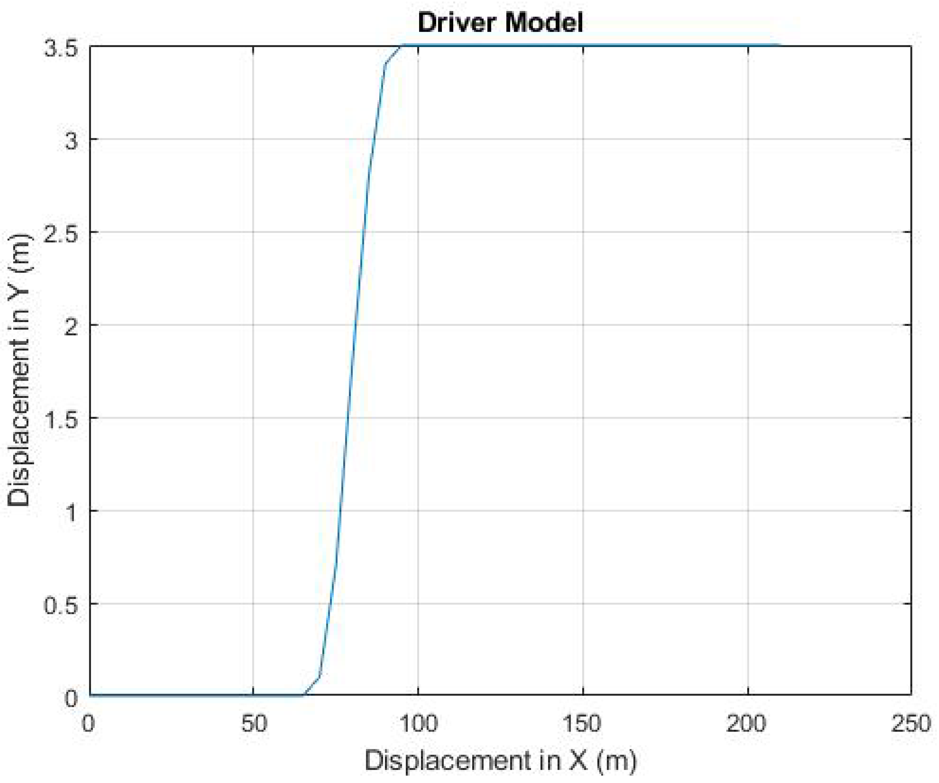
A predefined path is used to simulate the SLC maneuver and is shown in Figure 6. The maneuver is shown in 2D trajectory rather than in the more customary time and steering angle view. In real life driving, regardless of the speed or driver reaction time, a defined single lane-change requires a car to move a fixed distance on the same road. Over the testing maneuver, the driver model will actively adjust its steering input in order to ‘drive’ the vehicle to follow the predefined trajectory, as opposed to the open-loop driving scenario.

The built-in driver model is an optimal preview driver model [32], which has been incorporated in the commercial software package, CarSim, for closed-loop simulations of road vehicles. The driver model was derived by minimizing a cost function defined as a mean squared error between a predicted and a target lateral position. Experiment and simulation results demonstrated that driver steering in path-following maneuvers can be accurately modeled as a time-delay optimal preview control.

Two parameters, i.e., vehicle forward speed (U) and reaction time (t) of the driver model, are used to generate the look-up table for the gain scheduling controller consisting of the driver’s reaction time and vehicle forward speed.

5.4. The Gain Scheduling Controller

A gain scheduling controller (GSC) is used when a non-linear system can be broken down into various linear operating ranges [33]. The control gain values, K, are determined for each of these operating ranges to create a look-up table. Based on environmental factors or internal operating conditions, the GSC chooses a set of values from the look-up table. This allows for a more robust non-linear control using linear techniques and gain scheduling. There are many variations of GSC based on how the parameters are varied [34], this research focused on the vehicle forward speed and driver reaction time to generate a two-dimensional look-up table.

There are four steps to design and implement a GSC [34].

Step 1: Breakdown the existing system into a number of linearized models, as needed. According to [34], a popular method to do this is the Jacobian linearization. However, the approach used in this research does not require mathematical linearization. By varying the speed and reaction time parameters in the CarSim model, the model is automatically updated, which is utilized to generate the optimal control gain matrix K for that particular scenario.

Step 2: Design a linear controller. The evolutionary optimized ATS controller is the linear control technique. This controller follows design constraints, natural selection, and biological evolution to generate the control gain matrix K.

Step 3: Develop a look-up table and a look-up scheme. This is the actual creation of the GSC. Each gain is scheduled based on vehicle forward speed and reaction time of the driver model. After the GDE3 optimizer terminates, an optimal Pareto-front is achieved. For each combination of vehicle forward speed and driver reaction time, there exists an optimal Pareto-front. To simplify the design, the best trade-off solution of each optimal Pareto-front is used to test the GSC.

Step 4: Evaluate the system’s performance and ensure that the GSC is working within the design variable ranges. The GDE3 optimized controller and a gain scheduling controller are compared to confirm correct functionality and to analyze the advantages.

The GSC works based on a two-dimensional look-up table. The first independent variable is the variation of vehicle forward speed, and the second independent variable is the reaction time of the driver model.

Table 4. GSC look-up table.

Number of Setting Point	Forward Speed (km/h)	Reaction Time (s)
1	80	0
2	90	0
3	100	0
4	110	0
5	120	0
6	80	0.1
7	90	0.1
8	100	0.1
9	110	0.1
10	120	0.1

shows all possible combinations of the vehicle forward speed and driver reaction time that are taken into consideration in the GSC.

The GSC is a two-dimensional discrete decision algorithm so an important issue is the scheme to switch between different modes of operation. In this work, two switching schemes are tested. Firstly, controller gains are changed when the speed increases beyond the next discrete step, e.g., controller gains shifts from those associated with 80 km/h to 90 km/h if the speed goes to or beyond 90 km/h. The second scheme changes gains when the speed of the vehicle is rounded to the nearest speed value, e.g., mode shifts from 80 km/h to 90 km/h when the speed crosses 85 km/h. The performance in both cases is seen to be similar but when using the first scheme the overall number of times the gains change is less than the second.

5.5. GSC Modular Design Methodology

In this research work a co-simulation environment is built that combines CarSim with MATLAB/Simulink. CarSim software offers an integrated S-Function interface for the Simulink software package. The S-function data are sent and received by CarSim. The simulation results are directly captured from the CarSim model. This eliminates the chance of modeling errors and ensures the soundness of the results.

The system model shown in Figure 7 is highly modular. An important principle of this research is to ensure that the GSC design method is not system-specific. The system model is based on 5 main blocks. The CarSim block holds the car–trailer model, driver-model and all built-in testing maneuvers. It also provides the simulation results, which are fed into the control module. The evaluation block receives the simulation results from CarSim and assigns fitness values based on performance measures. If the fitness values exceed or violate the constraints, they are excluded from the simulation. The optimization module receives the fitness costs and uses them to assign fitness to population members for carrying out the evolutionary algorithm and generating new population members. The control module uses the optimal solutions from the optimization module to generate control gain matrix K which is then fed as the ATS system’s steering angle to CarSim. Each of these blocks can be changed depending on applications. The evaluation method, constraints, optimization techniques, control strategies, and car–trailer model can all be tailored to any system.

The CarSim model receives adjustable control input values every time a new speed or driver model reaction time is introduced. This validates the modularity of the CarSim block. The constraint module ensures that, above all, the control gain value must be able to stabilize the system during the complete maneuver. The car–trailer combination must follow the predefined path, without violating road boundaries. The maximum allowed RWA of the car–trailer combination is $2.0$. The optimization module in our case is the GDE3 algorithm and the control module is an LQR ATS controller.

6. Simulation Results and Discussions

In this section, we present the results of an optimized LQR controller for the car–trailer combination with ATS presented in Section 5 based on the vehicle’s performance in terms of PFOT and RWA values for different speeds and driver reaction times. The first set of results are the Pareto front graphs showing the optimal values for K with respect to the PFOT and RWA ideal values. The second set of results demonstrate the vehicle’s PFOT and RWA values for three different optimized K values (minimum PFOT, ideal RWA and the trade-off PFOT and RWA) and compares these results to the ideal and the vehicle without ATS. The third set of results show the performance of the vehicle when the gain scheduler is applied for different vehicle speeds as compared to the ideal and trade-off PFOT and RWA trajectory results.

6.1. GDE3 Optimal Pareto Fronts

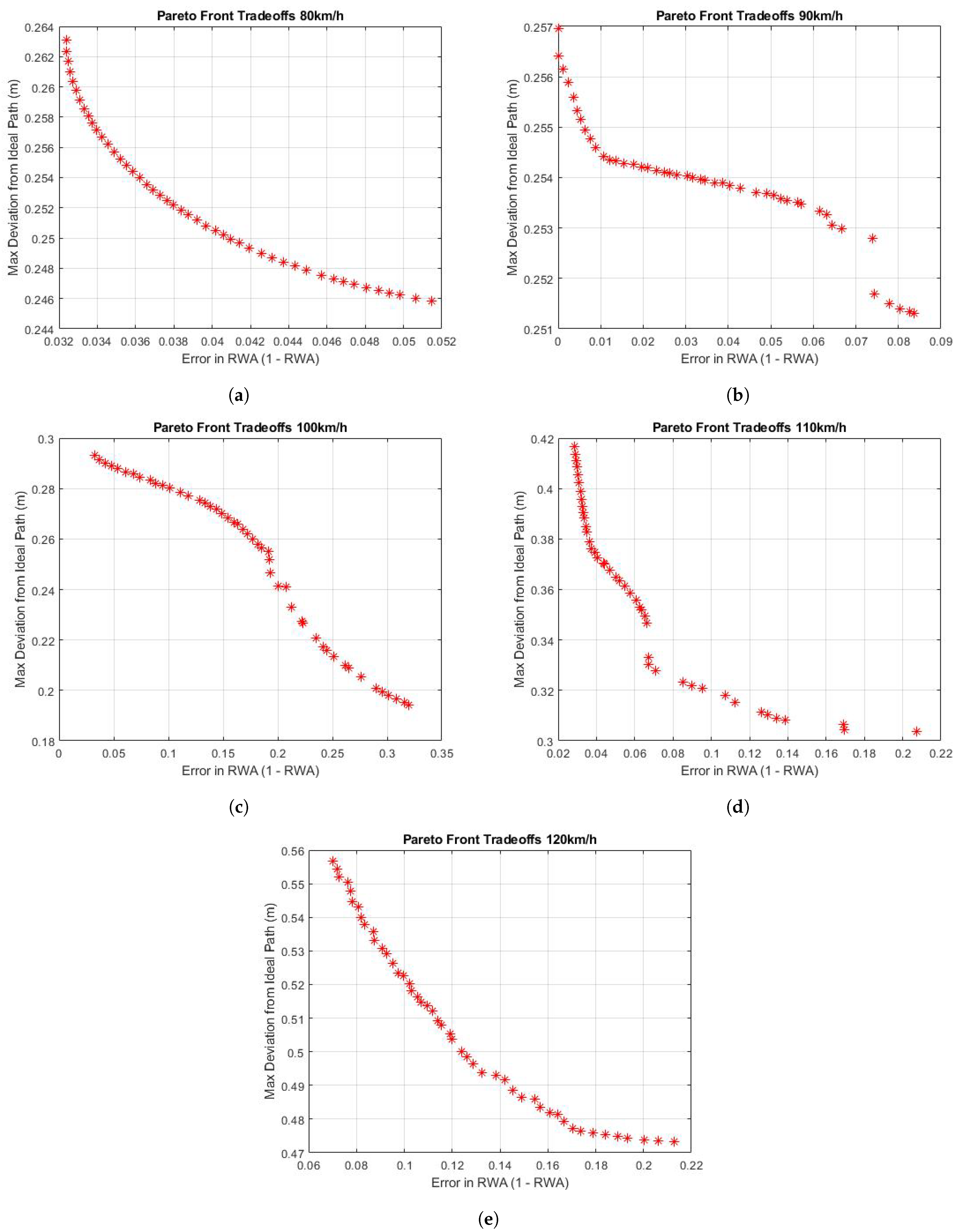
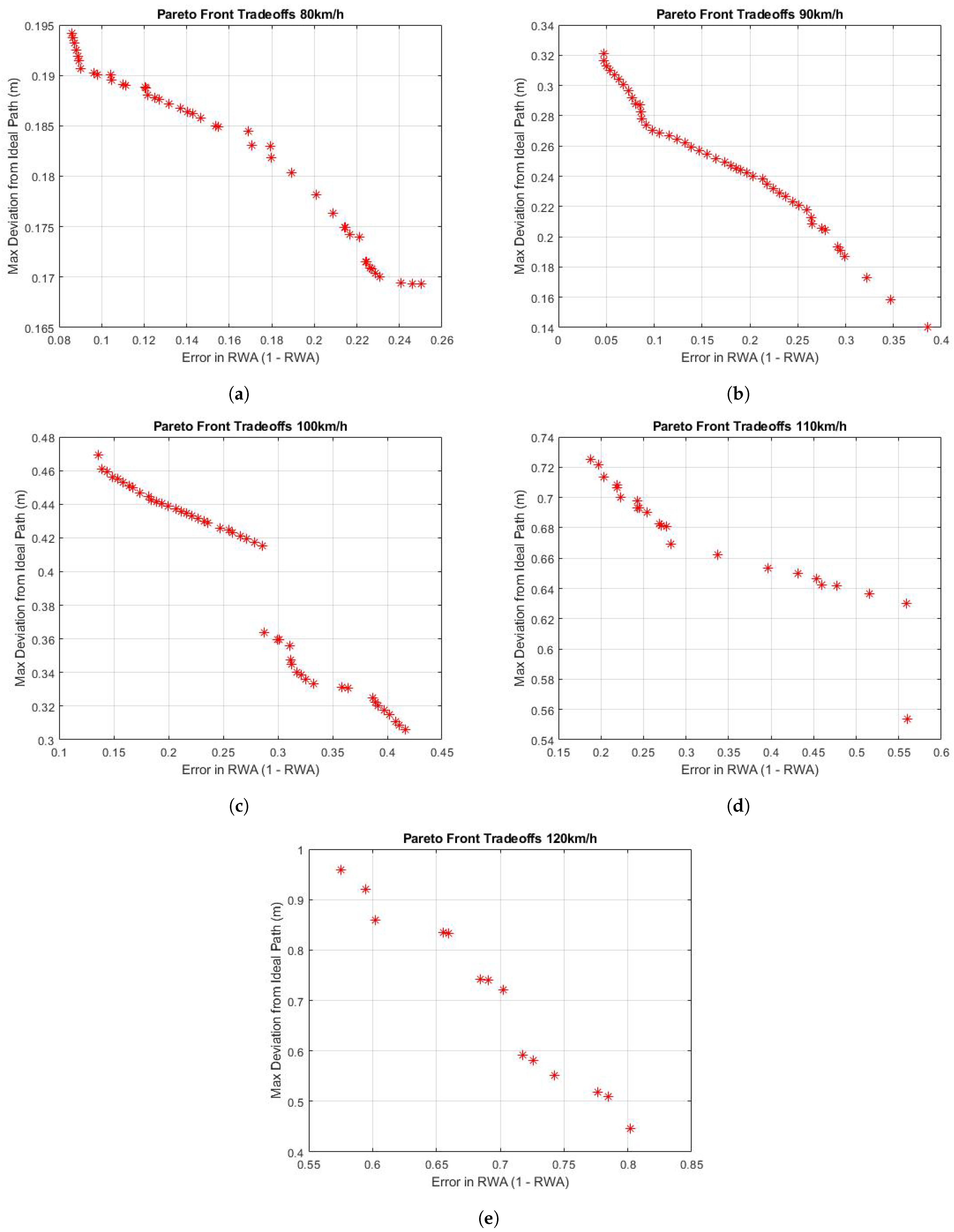
For the vehicle forward speeds and reaction delay times shown in Table 4 it is possible to determine 10 Pareto-front graphs showing the optimal values for K with respect to the PFOT and RWA ideal values. These Pareto-front graphs are shown in Figure 8 and Figure 9. It should be noted that the reaction time of 0.1 s is selected following the Best Path Tracking area recommended in [23], while the reaction time of 0 s is chosen assuming that the driver model is used as an automated steering controller with negligible reaction time.

Figure 8 and Figure 9 illustrate the Pareto-front graphs when vehicle forward speeds are 80, 90, 100, 110, and 120 km/h, while the driver’s reaction time is 0.0 and 0.1 s, respectively. Although there are minor differences among the shapes of these Pareto-front graphs, all these graphs share a common feature that the overall trade-off relationship between the design criterion of PFOT and (1-RWA) is clearly indicated. This trace-off relationship will facilitate the analysis and selection of potential compromised solutions.

For all of these Pareto-front graphs there are three main points of interest: the two utopia points (extreme points that represent optimal PFOT and RWA) and the trade-off solution. The trade-off is a decision to be made by the system designer, but in our examples we chose the the point which has the best compromise between the minimal PFOT and ideal RWA objectives.

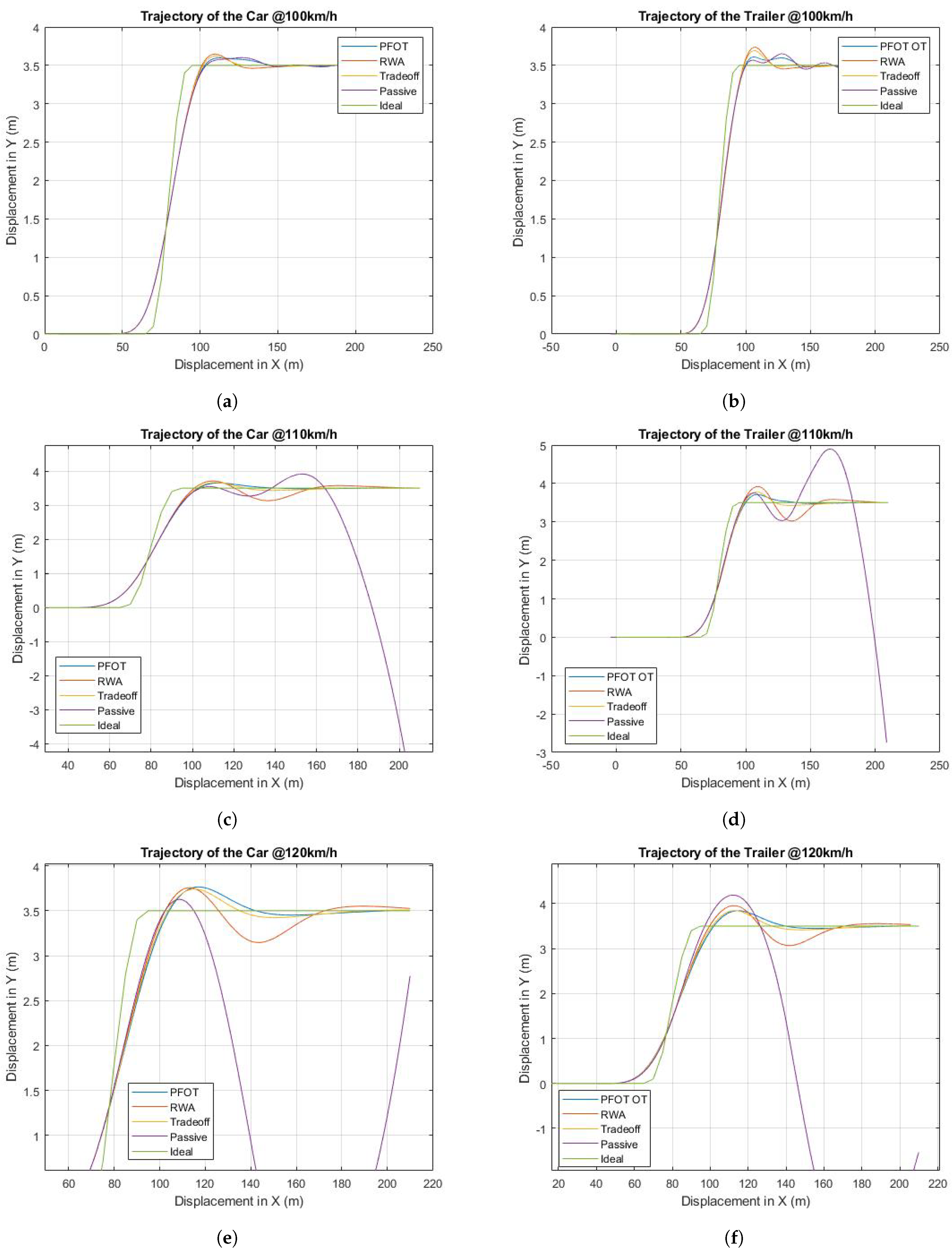
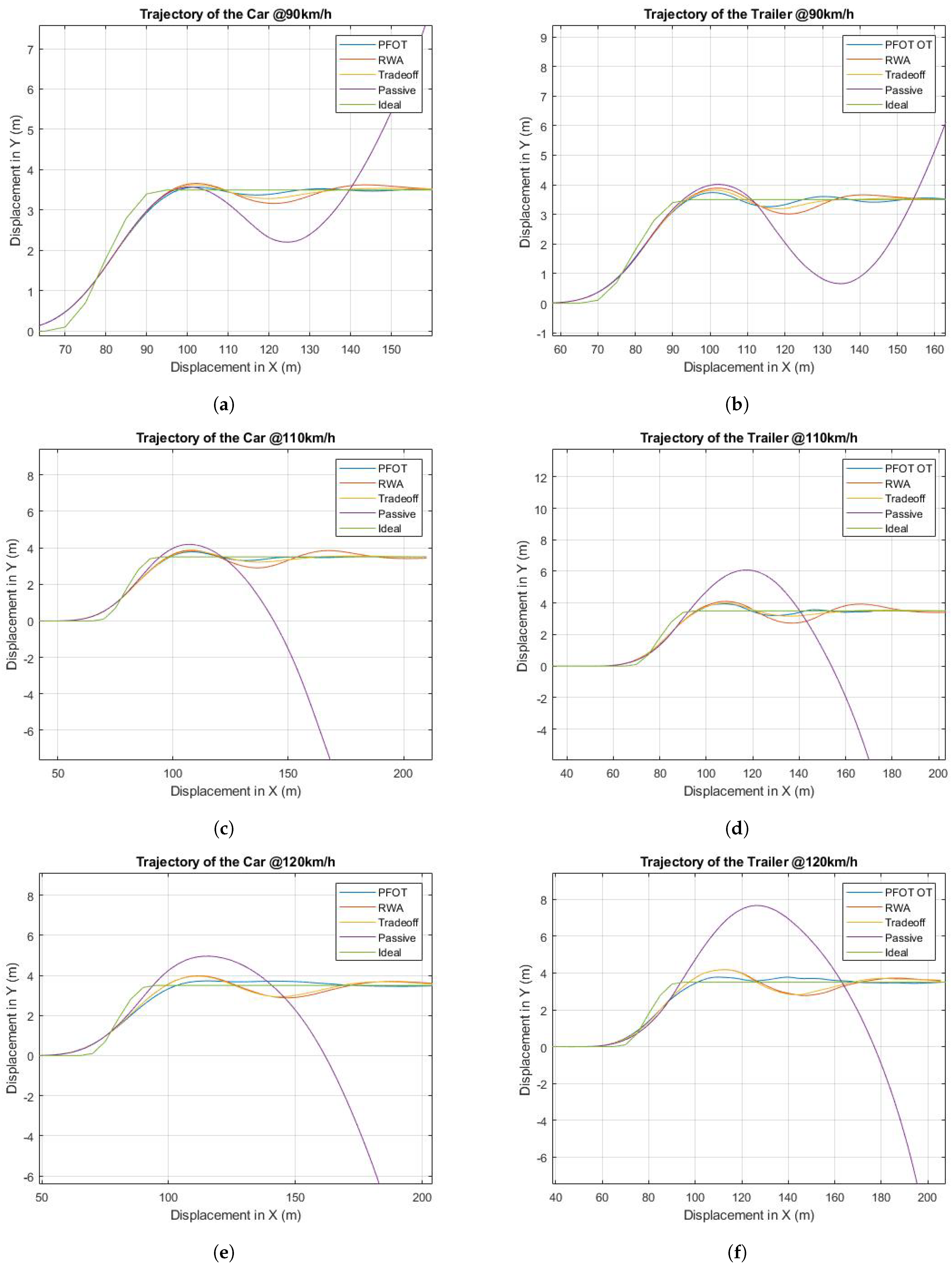
For all 10 vehicle speed and reaction time combinations listed in Table 4, we performed the SLC maneuver shown in Figure 6 for gains corresponding to an optimized PFOT (a utopia point), optimized RWA (the other utopia point), the trade off point, and the passive system without ATS. These results are shown in Figure 10 and Figure 11. For these graphs the ideal SLC path is also included for reference. In Figure 10, car and trailer tracking results are shown commencing at a vehicle speed of 100 km/h as the results at the lower speeds are fairly stable. For Figure 11 results are shown commencing at a vehicle speed of 90 km/h as the tracking performance degrades significantly for the passive case at this speed and higher. It should be noted that in Figure 10 and Figure 11, with respect to the case of passive (without active trailer steering), the differences among the curves corresponding to the cases of PFOT, RWA and Trade off appear not evident. This implies that compared with the passive design without ATS, the three ATS design solutions show much better performance although there exist evident differences among the three ATS designs. A close observation of Figure 10e indicates that among the three ATS designs, the PFOT shows the best overall trajectory-tracking performance, and the RWA exhibits the worst trajectory-tracking performance.

We summarize our observations as follows. As vehicle speed increases, the benefit of the optimized ATS controller becomes more apparent. Above the vehicle speed of 100 km/h, the passive system completely fails to complete the maneuver when the driver model reaction time is 0 seconds, and fails at 90 km/h when the driver model reaction time is set to $0.1$ s. The GDE3 optimized ATS controller is able to stabilize the system and to complete the SLC maneuver for all ten scenarios. At this point one could wrongly assume that any optimized K value could be chosen for the controller but at vehicle speeds of 120 km/h the car–trailer combination optimized RWA value is about $0.45$ for a driver reaction time of 0.01 s. In all other cases the optimal RWA values are close to the ideal value of $1.0$.

A limitation of the use of the CarSim model is that at most it can only support up to 1500 generations by the optimizer. This greatly reduces the time and opportunity for the algorithm to search the solution space.

6.2. Performance of the Gain Scheduling Controller

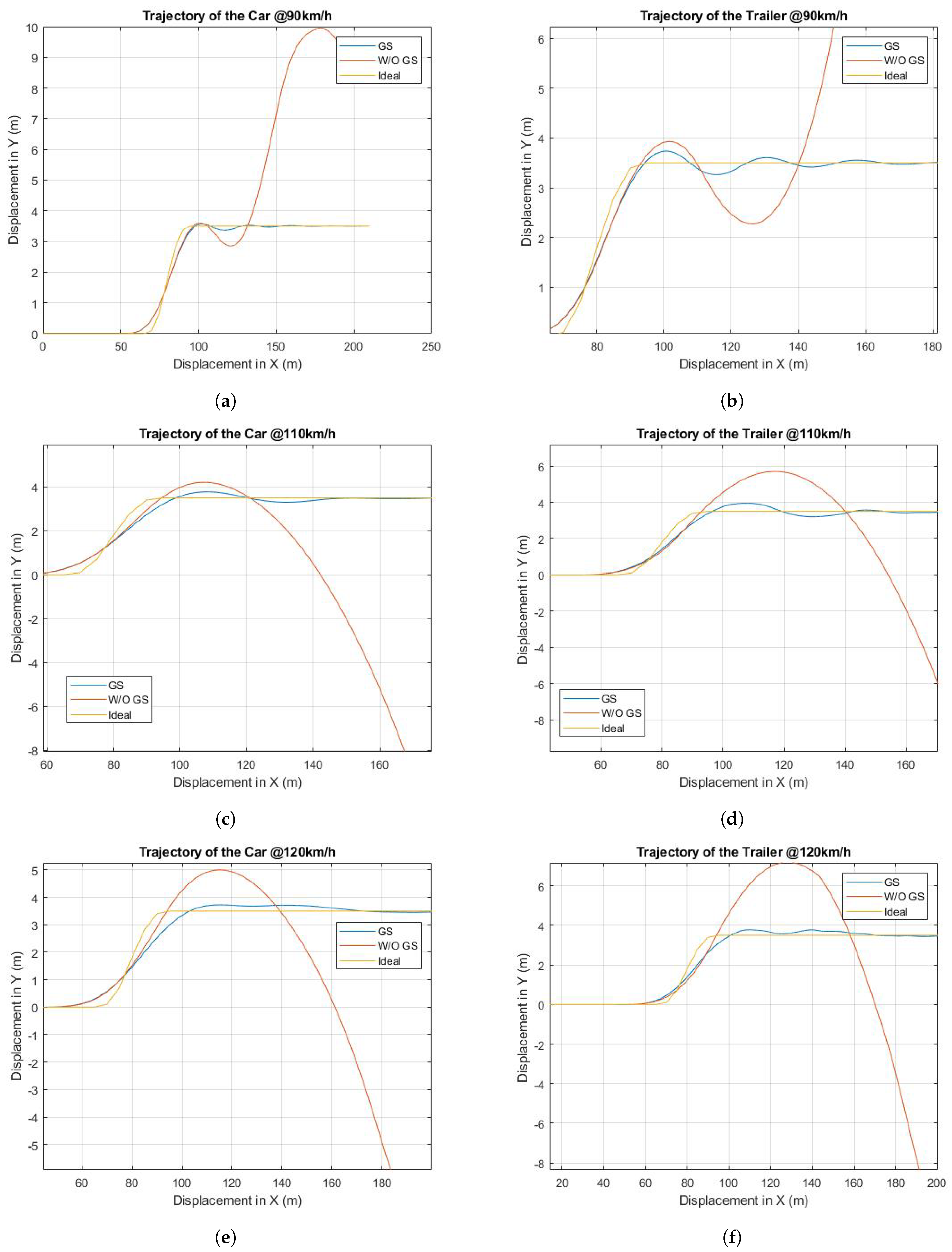
In this last section we demonstrate, using the aforementioned results, how the gain scheduling controller (GSC) further improves the ATS system. The GSC is compared to a GDE3 optimized ATS tuned at 100 km/h with a 0 s driver model reaction time (referred to as “W/O GS” in the graphs.) For brevity only the results are presented for vehicle speeds from 90 to 120 km/h for a driver model reaction time of 0.1(s) as these scenarios are the worst conditions. The control gains K is chosen such that the trajectory is optimized for the lowest PFOT and a RWA value closest to one. The results of these experiments is shown in Figure 12 and summarized in

Table 5. RWA comparison GS vs. W/O GS.

Speed (km/h)	Reaction Time (s)	GS	W/O GS	Improvement (%)
80	0.0	1.0751	1.1749	8.49
90	0.0	1.0929	1.2662	13.69
110	0.0	1.2072	1.3120	7.99
120	0.0	1.3626	3.3314	59.03
80	0.1	1.2503	1.2770	2.09
90	0.1	1.3853	1.9563	29.19
100	0.1	1.4168	3.2507	56.42
110	0.1	1.5600	3.2304	51.71
120	0.1	1.8018	3.3320	45.92

.

Overall the use of the GSC has a great advantage over using the LQR controller tuned for only a specific speed. For lower speeds, the improvement is not as apparent by looking at just the trajectory, but looking at Table 5 the improvement is more apparent as the values for RWA are significant lower than those when the GS is not utilized.

The GSC is a two-dimensional discrete scheme so it is important to know when to switch between different modes of operation. In this work, we tried to find methods of switching, in the first the controller gains are changed when the speed increases beyond the next discrete tens decimal step (controller gains shifts from those associated with 80 km/h to 90 km/h if the speed goes to or beyond 90 km/h) and in the second scheme gains are changed when the speed crosses the mid point between 2 tens decimals (mode shifts from 80 km/h to 90 km/h when the speed crosses 85 km/h.) The performance in both cases is seen to be similar but when using the first scheme the overall number of times the gains change is less than the second.

7. Conclusions

In this research we leveraged the GDE3 evolutionary algorithm to optimize the gains of an LQR controller for a car–trailer combination with active trailer steering. The car–trailer combination incorporated a driver in the loop model with a reaction time delay of 0.1 s. The scenario focused on a multi-objective design optimization process that demonstrated the trade off between optimizing the LQR controller path following objective for low speeds and rear-ward amplification objective for high speeds.

A multi-objective tuned gain scheduling controller (GSC) was designed for car–trailer combinations. The GSC was designed using the LQR control technique considering the variation of vehicle forward speed. A set of control gain matrices were used as the look-up tables for the GSC. The GSC outperforms passive system without ATS and managed to keep the vehicle within the ideal RWA value of 1.0 up to a vehicle speed of 120 km/h. We observed similar positive tracking results that are close to the ideal scenario for the PFOT objective for varying vehicle speeds and driver reaction times.

Although the proposed LQR-based gain scheduling controller (GSC) was designed for active trailer steering control for car–trailer combinations, the design method is also applicable for articulated heavy vehicles with tractor/semitrailer combinations. In the LQR-based GSC design, other uncertainties, e.g., trailer payload, may also be considered as vehicle forward speed discussed in this study. Due to the trailer tire cornering force saturation at high lateral accelerations, the proposed active trailer steering system is only effective in low lateral acceleration range, e.g., less than 0.40 g. The proposed LQR-based ATS scheme is suited for both cases of autonomous driving and human driver driving.

The maneuvers simulated in this paper are for a closed-loop single lane-change at a constant vehicle forward speed. A new testing maneuver may be designed, which incorporates variable vehicle forward speeds. This maneuver, with a greater speed sensitivity, may be used to further improve and test the GSC. The research into the maneuver, which may accurately depict and test a GSC, is a great step towards creating a robust ATS control system.