Research on Tire–Road Parameters Estimation Algorithm for Skid-Steered Wheeled Unmanned Ground Vehicle

Abstract

Skid-steered wheeled vehicles can be applied in military, agricultural, and other fields because of their flexible layout structure and strong passability. The research and application of vehicles are developing towards the direction of “intelligent” and “unmanned”. As essential parts of unmanned vehicles, the motion planning and control systems are increasingly demanding for model and road parameters. In this paper, an estimation method for tire and road parameters is proposed by combining offline and online identification. Firstly, a 3-DOF nonlinear dynamic model is established, and the interaction between tire and road is described by the Brush nonlinear tire model. Then, the horizontal and longitudinal stiffness of the tire is identified offline using the particle swarm optimization (PSO) algorithm with adaptive inertia weight. Referring to the Burckhardt adhesion coefficient formula, the extended forgetting factor recursive least-squares (EFRLS) method is applied to identify the road adhesion coefficient online. Finally, the validity of the proposed identification algorithm is verified by TruckSim simulation and real vehicle tests. Results show that the relative error of the proposed algorithm can be well controlled within 5%.

1. Introduction

Skid-steered wheeled vehicles are different from traditional Ackerman steering vehicles. They do not have a traditional steering mechanism, relying on the different wheel speeds between each side to achieve steering [1]. The arrangement of the transmission and the suspension system is flexible, which does not occupy too much space of the vehicle body, and the off-road mobility and all-region passability are good [2]. With the deepening of the research on “unmanned” and “intelligent” vehicles, the combination of unmanned ground vehicle (UGV) and skid-steered wheeled vehicle technology has become a research hotspot, and many corresponding products have been produced for the military, agricultural, and construction machinery fields. The representative UGVs are: the Crusher 6 × 6 wheeled UGV by America, the Mule High Mobility UGV by America, the RoBattle 6 × 6 UGV by Israel, the J6 XTR (6 × 6) and J8 XTR (8 × 8) UGV by Canada, and the spark articulated suspension UGV by China [3,4,5,6].

Compared with Ackerman-steered vehicles, skid-steered wheeled vehicles do not have too many geometric constraints, and their motion control is completely dependent on the interaction between wheels and the road. Therefore, the accurate estimation of the tire–road contact is necessary for motion control. The tire–road contact characteristics of skid-steered wheeled vehicles include tire load, road adhesion coefficient, and slip rate. In addition, tire parameters are also important factors affecting the vehicle control process, such as tire stiffness and sideslip angle, but these two parameters cannot be directly measured by sensors, so researchers have conducted a lot of work to estimate tire stiffness and sideslip angle.

The focus of this study is to propose an observation method that combines online with offline algorithms to estimate tire parameters and the road adhesion coefficient of the skid-steered wheeled UGV. Based on the 3-DOF dynamic model and the Brush nonlinear tire model, an offline tire parameters estimation algorithm based on the PSO algorithm and an online road adhesion coefficient estimation algorithm based on the EFRLS method are proposed for the skid-steered wheeled UGV. The validity of the algorithm is verified by TruckSim simulation and real vehicle tests.

The contributions of this study are summarized as follows:

(1)

The kinematics model and 3-DOF dynamic model of the skid-steered wheeled UGV are established;

(2)

An offline longitudinal and cornering stiffness estimation algorithm using the Brush nonlinear tire model is proposed based on the PSO algorithm with adaptive inertia weight;

(3)

According to the estimation results of tire stiffness, referring to the Burckhardt adhesion coefficient formula, an online road adhesion coefficient estimation algorithm is proposed based on the EFRLS method and the single-wheel dynamics model.

(4)

The effectiveness of the algorithm is verified by real vehicle experiments.

This paper is organized as follows: In Section 2, related works in recent years are reviewed; in Section 3, the kinematics model, the dynamics model of the platform, and the tire model are established; in Section 4, an algorithm based on online and offline observation is proposed to estimate the tire stiffness and road adhesion coefficient; in Section 5, the experimental and simulation verification tests are presented; and in Section 6, the conclusions and future studies are put forward.

2. Related Works

For skid-steered wheeled UGVs, accurate estimation of tire parameters and tire–road contact characteristics is of great significance for vehicle dynamics modeling and motion control. The research methods and status of tire stiffness and tire–road contact characteristics estimation are discussed in this section, which can provide a reference for the research in this paper.

2.1. Research Status of Tire Stiffness Estimation

For UGVs, the longitudinal stiffness and the cornering stiffness of the tire are the important factors that affect vehicle control, but these two parameters cannot be directly measured by sensors. Therefore, researchers have carried out a lot of research in tire stiffness estimation, to reduce the calculation cost and improve the overall performance of the vehicle control system.

Based on the transverse force of the tire information, Lian et al. [7] established a simplified lateral dynamic model, supplemented by a recursive least-squares regression model considering forgetting factors and constraints to achieve tire cornering stiffness estimation. Taking the estimated cornering stiffness as input, a nonlinear sideslip angle observer based on a first-order Stirling interpolation filter and a first-order low-pass filter was established. Lee et al. [8] used the dual Kalman filtering algorithm combined with dual GPS antenna system data to estimate the steering stiffness online. Wang et al. [9] proposed a fuzzy adaptive robust cubature Kalman filter (FARCKF) to estimate the vehicle sideslip angle and steering stiffness. The recursive least-squares method was applied to update the model parameters of FARCKF, and the Takagi–Sugeno fuzzy system was applied to adjust the process noise parameters in FARCKF. Based on the Bayesian method, Berntorp et al. [10] regarded the deviation from the nominal stiffness value as a Gaussian disturbance and applied the particle filter and marginalization to realize the adaptive measurement noise and process noise, to realize the real-time estimation of tire cornering stiffness. According to the tire longitudinal force difference generated between two sides by the yaw moment will affect the steering movement, Wang et al. [11] estimated the cornering stiffness by using the longitudinal force difference as input. Sierra et al. [12] defined effective steering stiffness as the ratio of two-axis lateral force to sideslip angle. Based on the time-domain and frequency-domain vehicle lateral dynamics model, the direct method and β-less method were used to estimate the sideslip stiffness. Pereira et al. [13] proposed a tire cornering stiffness estimation method based on Levenberg–Marquardt (LM), which combined the experimental and theoretical values of the yaw rate through LM to estimate the tire cornering stiffness.

2.2. Research Status of Tire–Road Contact Characteristics Estimation

For skid-steered wheeled UGVs, their motion control is completely dependent on the ground force on the tire. Therefore, the estimation of tire–road contact characteristics plays an important role in the dynamic control of skid-steered vehicles. The tire–road contact characteristics include road friction coefficient, road adhesion coefficient, slip rate, etc.

The estimation algorithm of tire–road friction coefficient has always been a research hotspot. There are many factors affecting the tire–road friction coefficient, such as the tire pressure, pattern, temperature, material, etc., and it also has a great relationship with the road surface [14]. El Tannoury et al. [15] considered that the tire–road friction coefficient is mainly related to the tire pressure and the effective radius. Assuming that the rolling resistance is linear with the speed at low speed and low load, the wheel angular velocity, speed, and torque signal were divided into certain and uncertain quantities to decompose the observed signal. The correction amount was introduced to make the algorithm converge. Finally, the sliding mode observer was constructed to estimate the effective radius and rolling resistance. Han et al. [16] took the influence of road roughness and road texture into consideration and proposed an estimation method of tire–road peak friction coefficient considering the effective contact characteristics between the tire and the three-dimensional road. The effective contact area ratio coefficient was introduced into the LuGre tire model to optimize the estimation method.

In addition to rolling resistance, scholars are more concerned with the estimation of road adhesion. In particular, in the off-road environment, the estimation of the road adhesion coefficient is particularly important [17]. Liu et al. [18] used a single-wheel dynamics model to estimate tire–road adhesion and used the Brush tire model to calculate the current road adhesion coefficient based on the μ–S curve based on the current slip ratio. Wang et al. [19] assumed the road conditions of the front and rear tires were the same. The difference in the slope of the μ–S curve between the front and rear wheels was considered to be the influence of tire parameters and then used the vehicle driving state to estimate tire adhesion. This method can estimate the road adhesion coefficient with various driving modes, but it ignores the differences in road adhesion coefficient on both sides. Shim et al. [20,21] used a priori experience to assume the road adhesion coefficient, and the vehicle dynamics model was used to predict the vehicle dynamics output parameters. According to the difference between the model prediction results and the real vehicle sensor parameters, the assumed road adhesion coefficient was corrected. Ghandour et al. [22] used the tire force calculated by the Dugoff model and the nonlinear optimization method to estimate the road adhesion coefficient. Villagra et al. [23] used a weighted Dugoff model to estimate the road adhesion coefficient. Nilanjan et al. [24] used a sliding mode observer and an improved Dugoff model to estimate the longitudinal speed and road adhesion coefficient using only the wheel speed input.

3. System Modeling

In this section, the kinematics model and the dynamics model are established. In order to simplify system modeling, we make the following assumptions [25]:

(1)

The UGV is driving on a flat road, and the six wheels of the UGV are in contact with the road;

(2)

The 3 wheels on the same side rotate at the same speed;

(3)

The vehicle load is uniformly distributed;

(4)

The influence of vehicle suspension is not considered.

3.1. Kinematics Model of Skid-Steered Wheeled UGV

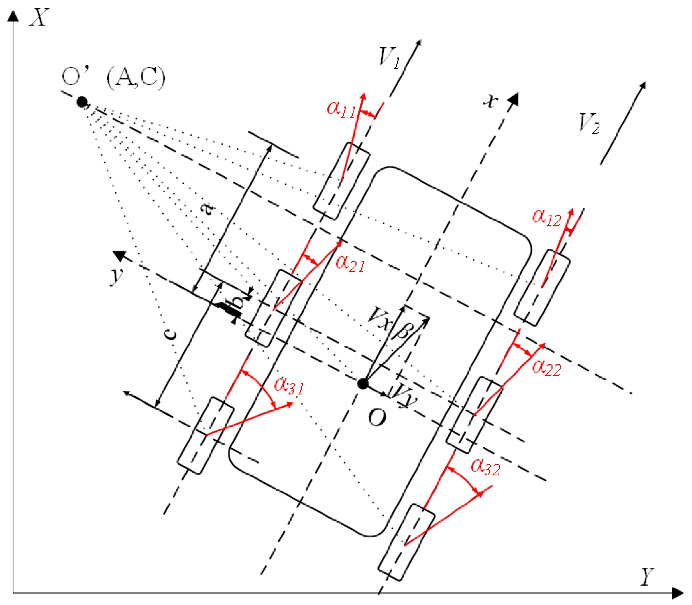
Due to the lack of geometric constraints similar to Ackerman-steered vehicles, the kinematic analysis is more dependent on the slip parameters. Based on the above assumptions, the kinematics diagram is established in Figure 1:

In Figure 1, a, b, and c denote the distance from each axis to the center of mass (CM).

In the vehicle body coordinate system, the kinematics equation can be expressed as:

$$\{\begin{array}{l}{v}_x=\frac{R}{2}\left[{\omega }_1\left(1-i_1\right)+{\omega }_2\left(1-i_2\right)\right]\\ v_y=\frac{R}{2}\left[{\omega }_1\left(1-i_1\right)+{\omega }_2\left(1-i_2\right)\right]\tan \beta =v_x\tan \beta \\ \dot{\varphi }=\frac{R\left[-{\omega }_1\left(1-i_1\right)+{\omega }_2\left(1-i_2\right)\right]}{B}\end{array}$$

(1)

where $v_x$ and $v_y$ denote the longitude and lateral velocity on the vehicle body coordinate; ${\omega }_1$ and ${\omega }_2$ denote the right and left side rotating velocity; $\dot{\varphi }$ denotes the yaw velocity; B denotes the width of the vehicle; R is the wheel radius; $\beta$ is the sideslip angle of the vehicle body; $s_1$ and $s_2$ denote the slip rate of each side wheel, which is expressed as:

$$s_j=\frac{R{w}_j-v_{xj}}{R{w}_j}$$

(2)

Based on Assumption (4), the longitude velocity of each side can be expressed as:

$$u_{x,ij}=\{\begin{array}{c}{v}_x-\frac{B}{2}\dot{\varphi } j=1\\ v_x+\frac{B}{2}\dot{\varphi } j=2\end{array}$$

(3)

The longitudinal slip rate can be expressed as:

$$\{\begin{array}{l}{s}_1=\frac{R{\omega }_1-\left(v_x-\frac{B}{2}\dot{\varphi }\right)}{R{\omega }_1}\hfill \\ s_2=\frac{R{\omega }_2-\left(v_x+\frac{B}{2}\dot{\varphi }\right)}{R{\omega }_2}\hfill \end{array}$$

(4)

The lateral velocity of the co-axial wheel can be expressed as:

$$u_{y,ij}=\{\begin{array}{ll}{v}_y+a\dot{\varphi }\hfill & i=1\hfill \\ v_y+b\dot{\varphi }\hfill & i=2\hfill \\ v_y+c\dot{\varphi }\hfill & i=3\hfill \end{array}$$

(5)

3.2. Dynamics Model of Skid-Steered Wheeled UGV

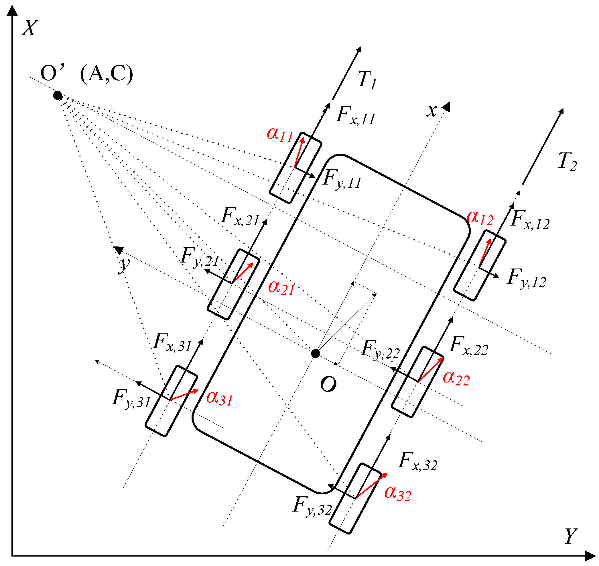
For the description of the planar motion of the skid-steered wheeled UGV, the multi-DOF nonlinear dynamics model can describe the motion state more accurately. In this study, the road roughness parameters are regarded as external disturbances, a 3-DOF nonlinear dynamics model of the skid-steered wheeled UGV is established, and the nonlinear tire model is used to describe the tire force. The force analysis of the vehicle is shown in Figure 2.

The 3-DOF dynamics model can be expressed as:

$$\{\begin{array}{l}m(a_x-v_y\dot{\varphi })={\displaystyle \sum _{i=1,2,3}{\displaystyle \sum _{j=1,2}{F}_{x,ij}}}\\ m(a_y+v_x\dot{\varphi })={\displaystyle \sum _{i=1,2,3}{\displaystyle \sum _{j=1,2}{F}_{y,ij}}}\\ I_z\ddot{\varphi }=\frac{B}{2}{\displaystyle \sum _{i=1,2,3}\left(F_{x,i1}-F_{x,i2}\right)}+{\displaystyle \sum _{j=1,2}\left(a{F}_{y,1j}+b{F}_{y,2j}+c{F}_{y,3j}\right)}\end{array}$$

(6)

where m denotes the mass of the vehicle; $a_x$ and $a_y$ denote the longitude and lateral acceleration on the vehicle body coordinate; $I_z$ denotes moment of inertia about the z-axis of the vehicle; $F_{x,ij}$ and $F_{y,ij}$ denote the longitude and lateral force on each tire.

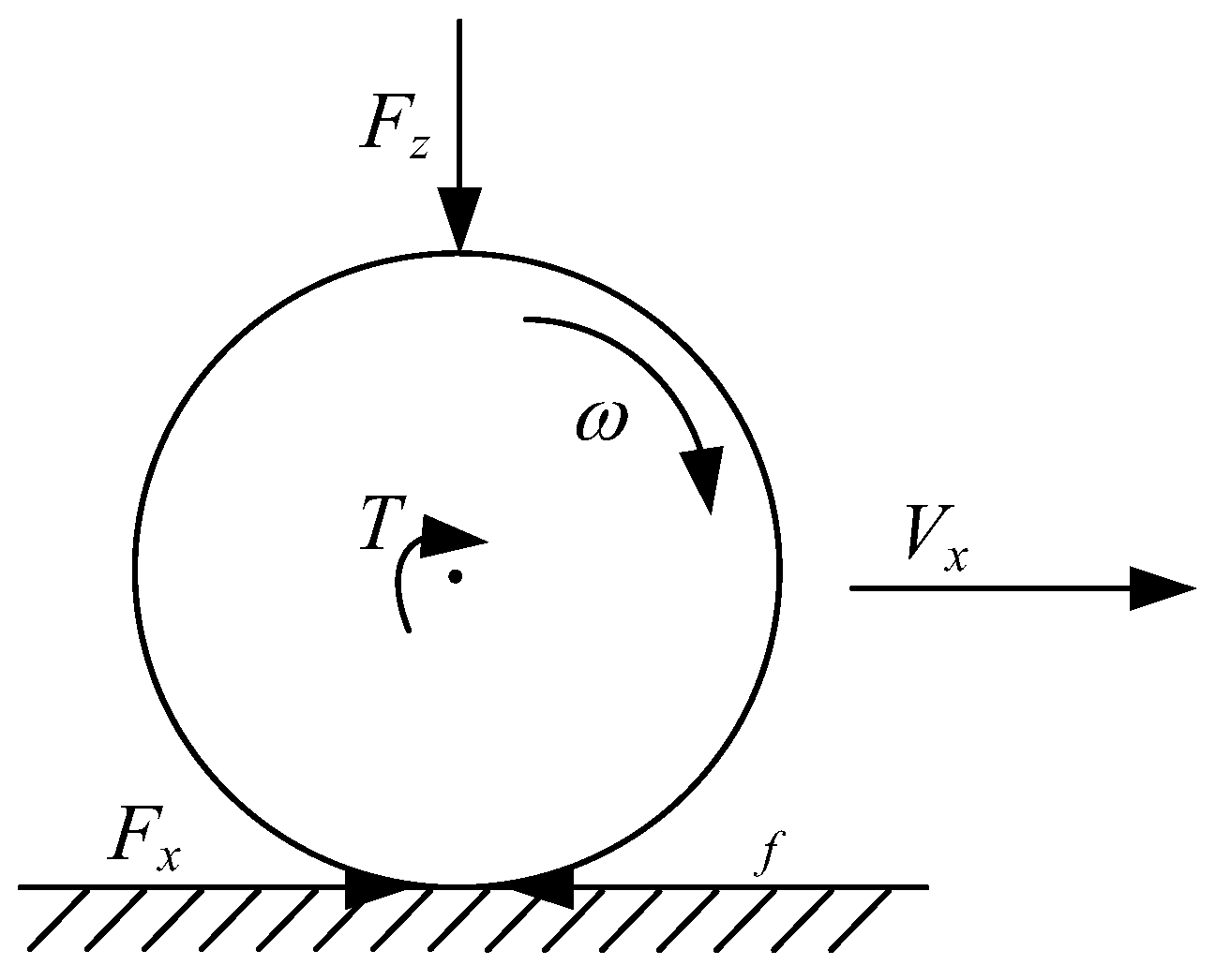
3.2.1. Single-Wheel Longitudinal Dynamics Model

In this study, the single-wheel longitudinal dynamics model is applied to identify the road adhesion coefficient. The single-wheel longitudinal dynamics model is shown in Figure 3

Then, the single-wheel longitudinal dynamics model can be expressed as:

$$I_w{\dot{\omega }}_{ij}=T_{ij}-R{F}_{x,ij}-R{f}_{ij}\hspace{1em}i=1,2,3;j=1,2$$

(7)

where $I_w$ denotes the moment of inertia of the wheel; ${\omega }_{ij}$ denotes the angular velocity of the wheel; $f_{ij}$ denotes the rolling resistance of the wheel; $i=1,2,3$ denotes the front, middle and rear wheels, respectively; $j=1,2$ denotes the left and right wheels, respectively.

3.2.2. Brush Nonlinear Tire Model

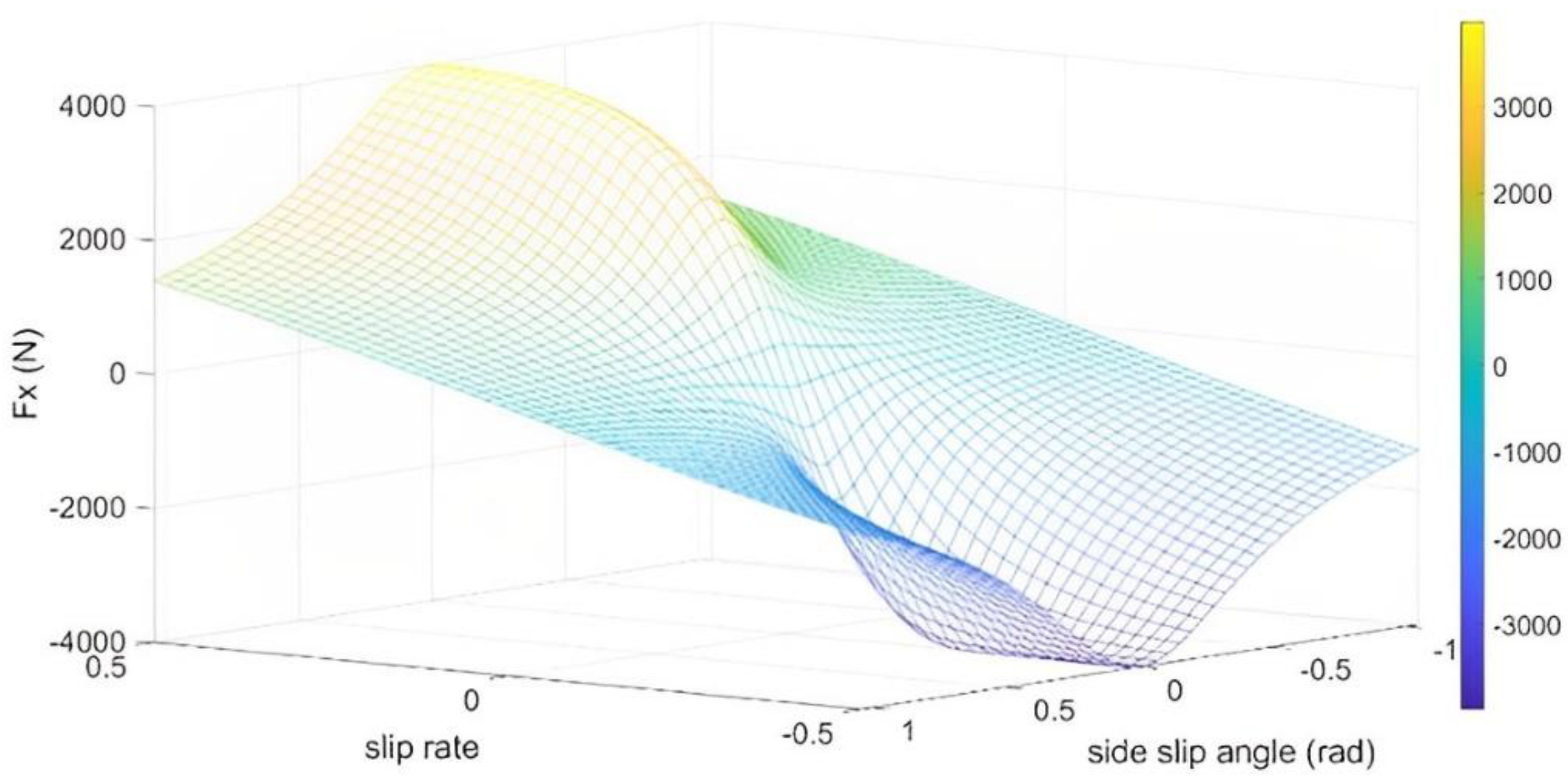
In this study, the Brush nonlinear tire model is applied to analyze the wheel-road contact characteristics of the vehicle. Considering the lateral–longitudinal combined slip characteristics of the tire, the contact between the tire and the road has comprehensive deformation stiffness and adhesion limit. The Brush nonlinear tire model is suitable for combined slip conditions, which assumes that the tire is a rigid ring surrounded by a ring of deformable brushes [26]. The model parameters are road friction coefficient $\mu$, longitudinal stiffness $C_x$, and cornering stiffness $C_{\alpha }$. The input is the longitudinal slip ratio $s$, sideslip angle, $\alpha$ and vertical load of the tire $F_z$.

The longitude and lateral force of the tire can be expressed as:

$$\{\begin{array}{l}s=\frac{R\omega -u_x}{u_x}\\ \alpha =\arctan \left(\frac{u_y}{u_x}\right)\\ C=\sqrt{C_x^2{\left(\frac{s}{1+s}\right)}^2+C_{\alpha }^2{\left(\frac{\tan \alpha }{1+s}\right)}^2}\\ F=\{\begin{array}{cc}C-\frac{1}{3\mu F_z}{C}^2+\frac{1}{27{\mu }^2{F}_z^2}{C}^3& C\le 3\mu F_z\\ \mu F_z& C>3\mu F_z\end{array}\\ F_x=\frac{C_{x}s}{(1+s)}\frac{F}{C}\\ F_y=-\frac{C_{\alpha }\tan \alpha }{(1+s)}\frac{F}{C}\end{array}$$

(8)

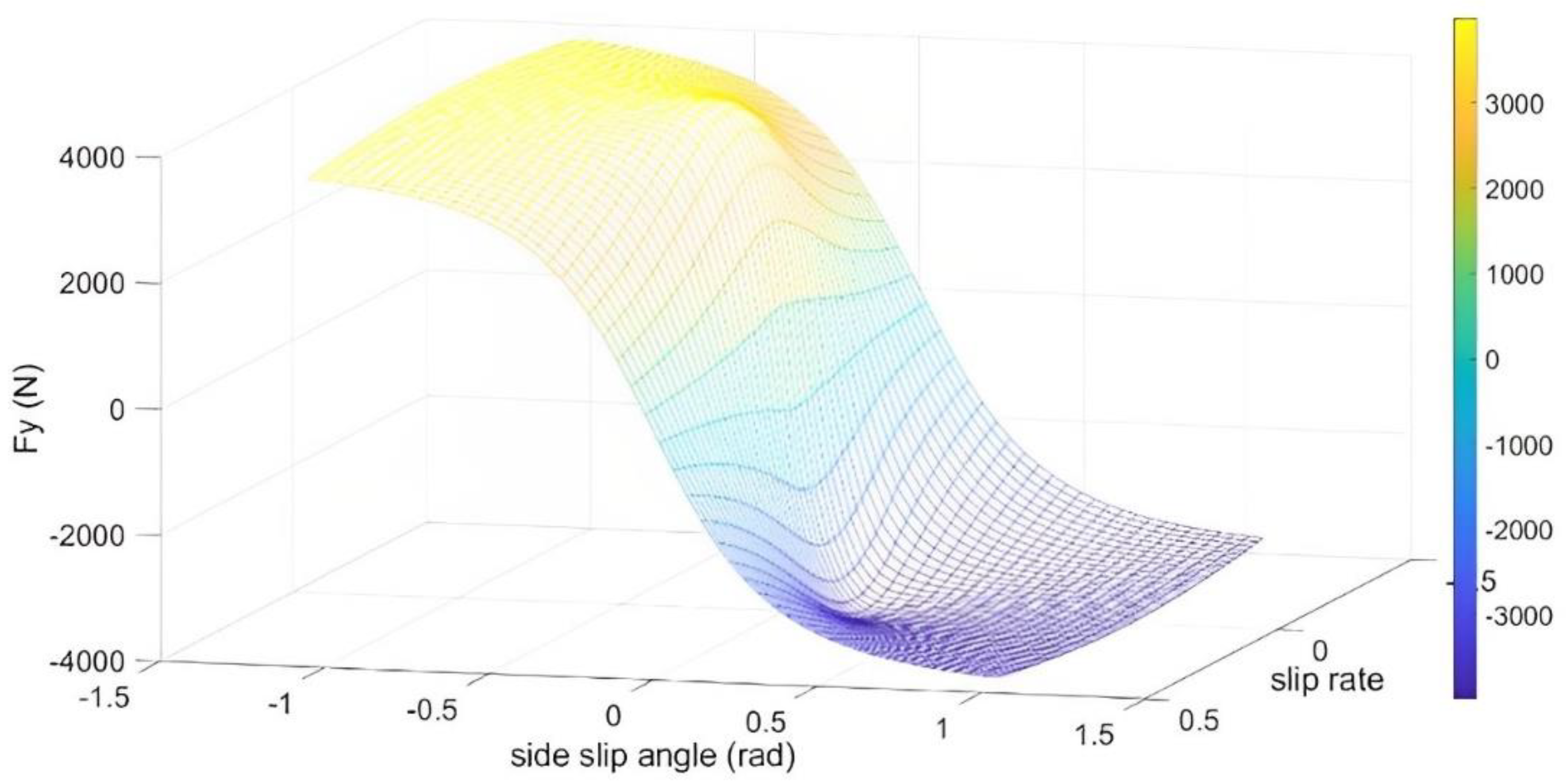
where $u_x$ and $u_y$ denote the lateral and longitudinal velocity of each wheel center, which can be calculated from (3) and (5). The longitudinal and lateral forces of the tire calculated by the Brush nonlinear tire model under the vertical load of 5000 N are shown in Figure 4 and Figure 5.

3.2.3. Vertical Force Estimation of the Tire

In this section, the longitudinal load transfer caused by vehicle acceleration and ramp conditions is discussed. The vertical load is divided into static load and dynamic load. The static load can be calculated according to the mass and the position of CM; dynamic load needs to consider the load change caused by the vehicle motion.

The tire force calculation for the multi-axes vehicle is a statically indeterminate problem. To calculate tire vertical force for the Brush nonlinear tire model, an assumption is proposed: the vertical deformation of the suspension and the tire follow a linear relationship, and the tire load is proportional to the vertical deformation of the suspension and the tire. Then, the tire vertical force in the longitudinal direction can be expressed as:

$$\begin{gathered} \{\begin{array}{l}{F}_{z1}=\frac{G\cos (\delta )\left(-a(b+c)+b^2+c^2\right) \\ +Gh\sin (\delta )(-2a+b+c)+hm{a}_x(-2a+b+c)}{2\left(a^2-a(b+c)+b^2-bc+c^2\right)}\\ F_{z2}=\frac{G\cos (\delta )\left(a^2-ab+c(c-b)\right) \\ +Gh\sin (\delta )(a-2b+c)+hm{a}_x(a-2b+c)}{2\left(a^2-a(b+c)+b^2-bc+c^2\right)}\\ F_{z3}=\frac{G\cos (\delta )\left(a^2-ac+b(b-c)\right) \\ +Gh\sin (\delta )(a+b-2c)+hm{a}_x(a+b-2c)}{2\left(a^2-a(b+c)+b^2-bc+c^2\right)}\end{array} \end{gathered}$$

(9)

where $F_{z1},F_{z2},F_{z3}$ denote the vertical force on the front, middle, and rear axis; h denotes the height of CM; G denotes the gravity of the vehicle; $\delta$ denotes the road gradient.

Take the lateral acceleration into consideration:

$$\Delta F_{z1}=-\Delta F_{z2}=\frac{m{a}_{y}h}{B}$$

(10)

where $\Delta F_{z1}$ and $\Delta F_{z2}$ denote the vertical load variation of the right and left sides due to the influence of lateral acceleration. Then, the vertical tire force can be expressed as:

$$F_{zij}=\{\begin{array}{c}\frac{F_{zi}}{2}-\frac{m{a}_{y}h}{3B}\hspace{0.17em}\hspace{0.17em}\hspace{0.17em}i=1,2,3\hspace{0.17em}\hspace{0.17em}\hspace{0.17em}j=1\\ \frac{F_{zi}}{2}+\frac{m{a}_{y}h}{3B}\hspace{0.17em}\hspace{0.17em}\hspace{0.17em}i=1,2,3\hspace{0.17em}\hspace{0.17em}\hspace{0.17em}j=2\end{array}$$

(11)

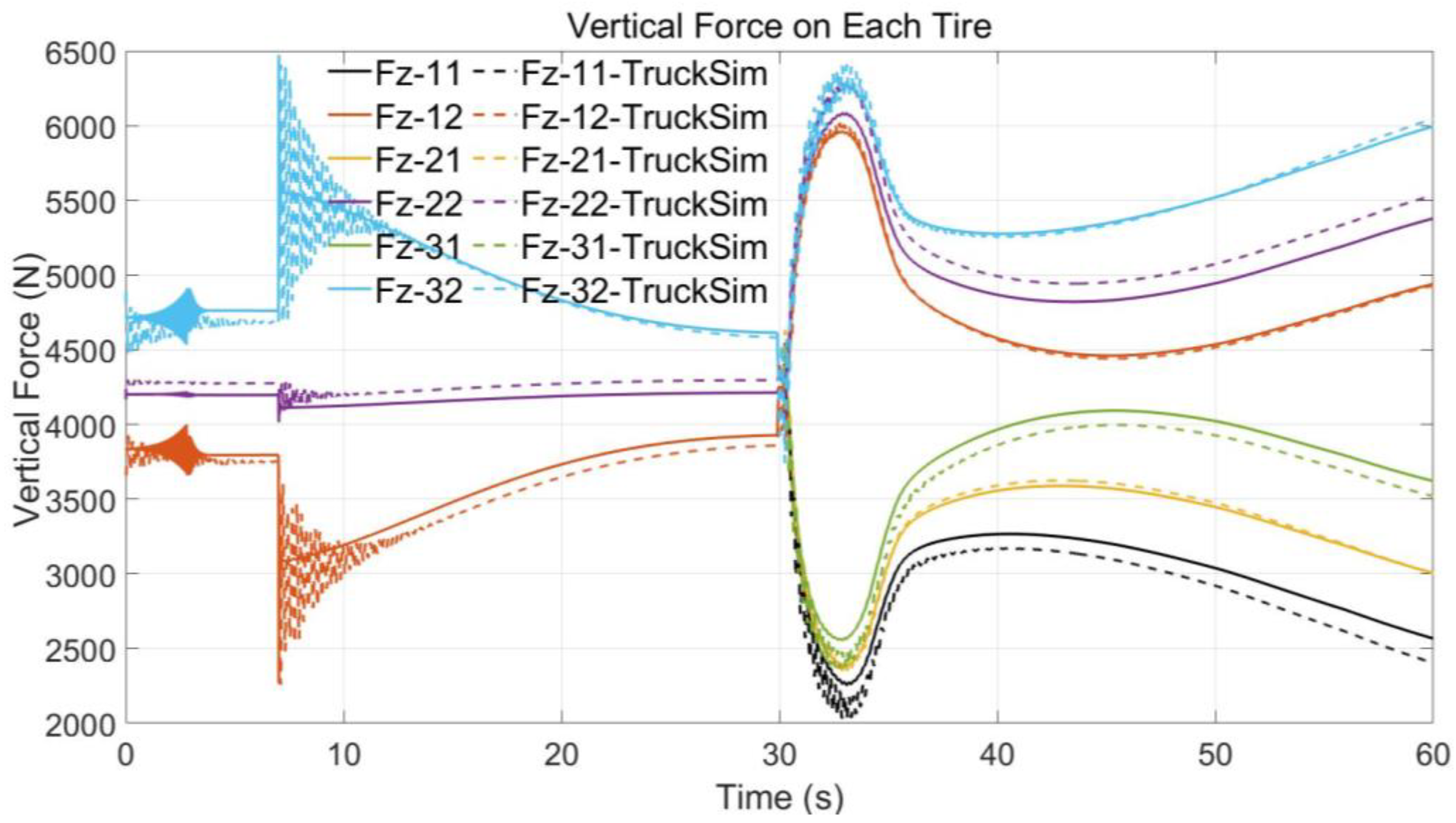
The simulation result in TruckSim is shown in Figure 6, which shows the change in the vertical load of each wheel during acceleration and steering. When the vehicle begins to accelerate from the 8 s, the vertical load on the rear axis increases and the load on the front axis is inverse. When the vehicle turns for 30 s, the vertical load on the right side increases, and the load on the left side is inverse. The simulation result shows the vertical force calculation method satisfies the accuracy requirement at different driving conditions.

4. Observer Design

For the skid-steered wheeled UGV applied to variable conditions, the ability to estimate the tire parameters and road parameters is necessary for the motion planning and control systems. The tire parameters are almost unchanged with the driving conditions during the actual driving, the offline identification method can be used to estimate the parameters. However, the road adhesion coefficient changes in real-time during the actual driving, which directly affects the motion control of the UGV, so an online identification method to estimate the road adhesion coefficient is necessary.

4.1. Offline Tire Parameters Estimation Algorithm

The tire parameters are generally considered to be constant and will not change with the operating conditions of the vehicle, so the offline identification algorithm can be used to estimate tire parameters. In this study, the Brush nonlinear tire model is applied, and the parameters to be identified are the longitudinal stiffness $C_x$ and cornering stiffness $C_{\alpha }$ of the tire.

4.1.1. Longitudinal Stiffness Estimation Algorithm

The straight driving condition is commonly chosen to estimate the longitudinal stiffness, to eliminate the influence of tire cornering condition. For the Brush nonlinear tire model, when the slip ratio of the tire is very small, the longitudinal stiffness of the tire can be approximately linear. When the vehicle acceleration is small, the longitudinal force of the tire can be approximated as:

$$F_{x,ij}=C_x{s}_{ij}$$

(12)

For the longitudinal dynamics model of the vehicle, it can be considered that the parameters of each tire are the same because of the same type of each tire, then the longitudinal dynamics equation can be expressed as:

$$m{a}_x=C_x{\displaystyle \sum _{\begin{array}{l}i=1,2,3\\ j=1,2\end{array}}{s}_{ij}}-F_r$$

(13)

where $F_r$ denotes the combined resistance of the vehicle, including the rolling resistance and wind resistance. This can be transformed into an optimization problem:

$$\begin{array}{l}\min J=\Vert \frac{1}{m}{\widehat{C}}_x{\displaystyle \sum _{\begin{array}{l}i=r,l\\ j=f,m,r\end{array}}{s}_{ij}-\left(a_x+\frac{F_r}{m}\right)}\Vert \\ st C_{x\min } \le C_x\le C_{x\max }\end{array}$$

(14)

The constraints of longitudinal stiffness determined by prior experience.

4.1.2. Cornering Stiffness Estimation Algorithm

For the traditional Ackerman-steered vehicle, the method of unpowered fixed steering wheel angle is commonly applied to estimate the cornering stiffness, which can eliminate the influence of longitudinal driving force. For the skid-steered wheeled vehicle, the steering mechanism determines that the skid-steered wheeled vehicle cannot realize the steering condition without power. The estimation of the cornering stiffness of the skid-steered wheeled vehicle must be carried out in the presence of longitudinal driving force. Therefore, the estimation of the cornering stiffness of the skid-steered wheeled vehicle must be based on the premise that the longitudinal stiffness of the tire is known. In this case, the method similar to the Ackerman-steered vehicle to take a large radius without power cannot be applied to make a linear assumption for the lateral condition of the tire. The longitudinal characteristics of the tire must be taken into consideration and the nonlinear estimation method of lateral and longitudinal coupling will be adopted.

In this study, the cornering stiffness of the tire is estimated by the tire model and vehicle cornering dynamic model under the premise that the longitudinal stiffness of the tire is estimated by the algorithm provided above. Under the premise that the longitudinal stiffness is known, the lateral force can be calculated by Equation (8). In addition, if the longitudinal slip ratio and sideslip angle of the tire are known, then the cornering stiffness estimation will be transformed into a nonlinear optimization problem:

$$\begin{array}{l}\min J=\Vert \frac{1}{m}{\displaystyle \sum _{\begin{array}{l}i=1,2,3\\ j=1,2\end{array}}{\widehat{F}}_y\left({\widehat{C}}_{\alpha },s_{ij},{\alpha }_{ij}\right)-a_y}\Vert \\ st C_{\alpha \min } \le C_{\alpha }\le C_{\alpha \max }\end{array}$$

(15)

where ${\widehat{F}}_y$ denotes the estimated value based on the estimated cornering stiffness ${\widehat{C}}_{\alpha }$. The constraints of cornering stiffness determined by prior experience.

4.1.3. Tire Stiffness Offline Estimation Algorithm Based on PSO

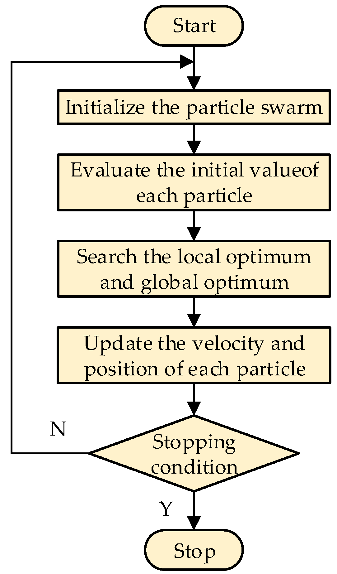
In this study, the particle swarm optimization (PSO) algorithm is adopted to estimate tire stiffness. The PSO algorithm is based on the randomness of the population parallel optimization algorithm. Compared with other algorithms, the PSO algorithm is more flexible, which does not need to identify the functions of differentiable or continuous, and does not need crossover or mutation operations. In addition, the tire of the skid-steered wheeled UGV is easy to be in a strong nonlinear condition during the steering process, and the PSO algorithm has better fitting performance for nonlinear conditions. The parameters that need to be adjusted in the PSO algorithm are less and the convergence speed is faster than other algorithms, so it has been widely used [27].

The traditional PSO algorithm is as follows: for the n-dimensional space, the total number of particles is N, ${\stackrel{\rightharpoonup }{X}}_i=[x_{i,1},x_{i,2}\dots x_{i,n}]$ denotes the i-th particle position vector, and ${\stackrel{\rightharpoonup }{V}}_i=[v_{i,1},v_{i,2}\dots v_{i,n}]$ denotes the velocity vector. By evaluating the objective function of each particle, the optimal position of a single particle ${\stackrel{\rightharpoonup }{P}}_i=[p_{i,1},p_{i,2}\dots p_{i,n}]$ and the optimal position of the entire particle swarm ${\stackrel{\rightharpoonup }{P}}_g=[p_{g,1},p_{g,2}\dots p_{g,n}]$ can be obtained. The velocity vector and position vector of each particle are then updated using the following equation:

$$\begin{array}{l}{v}_{i,j}^{m+1}=\gamma v_{i,j}^m+C_1{r}_1\left(p_{i,j}^m-x_{i,j}^m\right)+C_2{r}_2\left(p_{g,j}^m-x_{i,j}^m\right)\\ x_{i,j}^{m+1}=x_{i,j}^m+v_{i,j}^{m+1}\end{array}$$

(16)

where j = 1,2,…,n; m denotes the number of iterations; $r_1$ and $r_2$ are random values between [0,1]. $\gamma$ denotes non-negative inertia factors; the larger the value of $\gamma$ is, the stronger the global optimization ability of the algorithm is, and the weaker the local optimization ability is. $C_1$ and $C_2$ are non-negative constants, which are also parameters to adjust the weights of local optimal value and global optimal value.

The process of the PSO algorithm is as follows:

(1)

Initialize the particle swarm, including the number of particles, the initial velocity and position of each particle, and the inertia factor;

(2)

The evaluation function is adopted to evaluate the initial value of each particle in the particle swarm, the optimal position of each particle is saved, and the optimal solution is selected as the global optimal initial solution to record its position;

(3)

The velocity and position of the particles are updated according to Function (16);

(4)

Evaluate the updated particle swarm, update the local optimal value of each particle and the global optimal value of the whole particle swarm;

(5)

Repeat iteration steps (3) and (4) until iteration conditions are met.

The calculation process of the PSO algorithm is shown in Figure 7.

The problem with the traditional PSO algorithm is that the particles may converge at the local minimum. As the inertia factor, the greater the value of $\gamma$, the weaker the local optimization ability of the algorithm, and the stronger the global optimization ability; on the contrary, the smaller the value of $\gamma$, the stronger the local optimization ability of the algorithm, and the weaker the global optimization ability. Based on this, a linearly variable inertia factor is introduced into the PSO algorithm to simultaneously meet the algorithm’s requirements for global search and local accurate convergence with adaptive weight. The adaptive weight can be expressed as:

$$\gamma =\{\begin{array}{ll}{\gamma }_{\min }+\frac{\left({\gamma }_{\max }-{\gamma }_{\min }\right)\left(OF-O{F}_{\min }\right)}{O{F}_{\mathrm{avg} }-O{F}_{\min }}\hfill & OF⩽O{F}_{\mathrm{avg} }\hfill \\ {\gamma }_{\max }\hfill & OF>O{F}_{\mathrm{avg} }\hfill \end{array}$$

(17)

where $OF$ denotes the current objective function value of the particle; $O{F}_{\min }$ and $O{F}_{\mathrm{avg}}$ denote the minimum target value and the average target value of the particles, respectively.

From Function (17), for the adaptive weight, when the target value of each particle in the particle swarm tends to be consistent or tends to be local optimal, the inertia weight increases accordingly; when the target value distribution of each particle in the particle swarm is relatively dispersed, the inertia weight decreases accordingly. In addition, this algorithm can reduce the inertia weight of the particle whose target value is better than the average target value to retain the particle. The particles whose target values are worse than the average will get larger inertia weights so that these particles can move faster to better search space.

4.2. Online Road Adhesion Coefficient Estimation Algorithm

4.2.1. Slip Rate–Road Adhesion Coefficient Curve

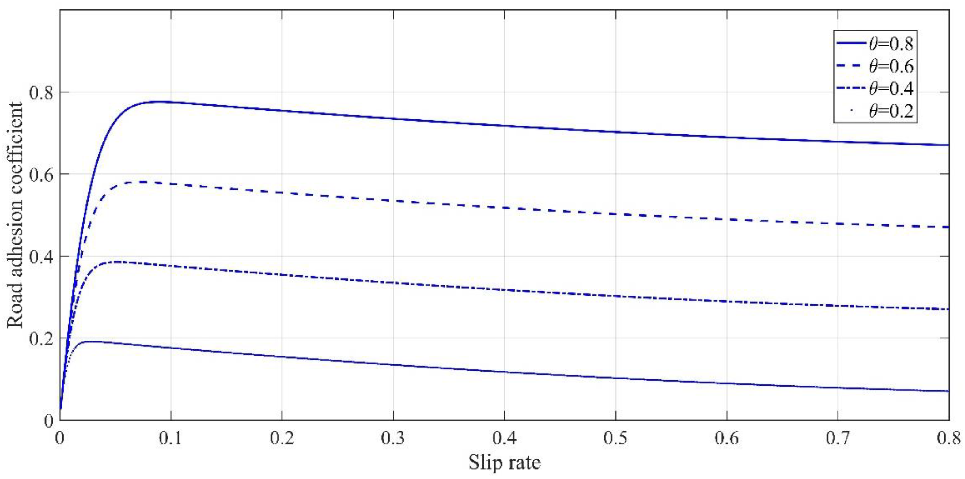
In this study, the road adhesion coefficient model proposed by Burckhardt [28] is adopted to estimate the road adhesion coefficient, which can be expressed as:

$$\mu (\theta ,\lambda )=\theta -\theta e^{-\frac{c_1}{\theta }\left(\lambda +c_2{\lambda }^2\right)}-c_3\lambda \mathrm{sgn}(\lambda )+c_4{\lambda }^2$$

(18)

where $\mu (\theta ,\lambda )$ denotes the utilization of road adhesion coefficient under the current tire load and slip rate; $\theta$ denotes the peak road adhesion coefficient; $\lambda$ denotes the tire slip ratio; $c_1$ defines the slope rate of the initial segment of the curve; $c_2$ is applied to adjust the slope rate of the curve without affecting the slope rate of the initial segment, $c_3$ and $c_4$ are used to adjust the decreased slope rate of the road adhesion coefficient after the maximum coefficient. Relevant experimental studies have found that the three coefficients $c_2-c_4$ have little effect on the slip rate–road adhesion coefficient curve, and the values under different road conditions also have little effect on the curve. Therefore, we generally take these three coefficients as fixed values in practical application, and the three coefficients calibrated by the test are $c_2=8, c_3=0.25, c_4=0.11$.

The influence of $\theta$ and $c_1$ on slip rate–road adhesion coefficient can be seen in Figure 8 and Figure 9. It can be seen that $c_1$ mainly affects the slope rate of slip rate–road adhesion coefficient before reaching the peak coefficient. Based on the above assumptions, this study will estimate the parameters in Equation (18) and $c_1$.

According to Equation (18), the slope rate of the road adhesion coefficient $\mu$ and slip rate $\lambda$ can be expressed as:

$$\frac{\partial \mu }{\partial \lambda }=c_1\left(1+2\lambda c_2\right)e^{-\frac{c_1}{\theta }\left(\lambda +c_2{\lambda }^2\right)}-c_3\mathrm{sgn}(\lambda )+2c_4\lambda$$

(19)

The slope rate of the road adhesion coefficient $\mu$ and $\theta$ can be expressed as:

$$\frac{\partial \mu }{\partial \theta }=1-\left[1-c_1\left(\lambda +c_2{\lambda }^2\right)\right]e^{-\frac{c_1}{\theta }\left(\lambda +c_2{\lambda }^2\right)}$$

(20)

According to Equation (19), let:

$$\frac{\partial \mu }{\partial \lambda }=0$$

(21)

Then, the slip rate ${\lambda }_s$ at the corresponding maximum road adhesion coefficient can be obtained, bringing ${\lambda }_s$ into Equation (18), the maximum road adhesion coefficient under current road conditions can be obtained. It is difficult to obtain the analytical solution with Equation (19), and the numerical solution can be obtained by the numerical method.

4.2.2. Road Adhesion Coefficient Estimation

In this section, the Brush tire model in Section 3 is applied as the tire model for the road adhesion coefficient estimation. The parameters to be estimated include the longitudinal stiffness $C_x$ and cornering stiffness $C_{\alpha }$ of the tire.

According to Equation (8), the 3-DOF dynamics model of the vehicle can be expressed as:

$$\{\begin{array}{l}m{a}_x={\displaystyle \sum _{\begin{array}{l}i=1,2,3\\ j=1,2\end{array}}{F}_{x,ij}\left(\mu \left(\theta ,c_1,{\kappa }_i,{\alpha }_i\right),F_{z,ij}\right)}-F_f-F_{air}\\ m{a}_y={\displaystyle \sum _{\begin{array}{l}i=1,2,3\\ j=1,2\end{array}}{F}_{y,ij}\left(\mu \left(\theta ,c_1,{\kappa }_i,{\alpha }_i\right),F_{z,ij}\right)}\\ I_z\ddot{\varphi }=\frac{B}{2}{\displaystyle \sum _{i=1,2,3}\left(F_{x,i1}-F_{x,i2}\right)}+{\displaystyle \sum _{j=1,2}\left(a{F}_{y,1j}+b{F}_{y,2j}+c{F}_{y,2j}\right)}\end{array}$$

(22)

In addition, the dynamic model of the wheel during vehicle driving is taken into consideration (Figure 3 and Equation (7)). For the test platform used in this paper, the wheel speed of the same side is the same, the longitudinal wheel speed of the same side is the same, and the three wheels on the same side are driven by the same motor, then the following dynamic equation can be obtained:

$$\{\begin{array}{l}3I_w{\dot{\omega }}_{wf}=\left(T_{m1}-{\displaystyle \sum _{i=1,2,3}{F}_{x,i1}\left(\theta ,c_1,{\kappa }_i,{\alpha }_i\right)R}-{\displaystyle \sum _{i=1,2,3}{F}_{f,i1}R}\right)\\ 3I_w{\dot{\omega }}_{wr}=\left(T_{m2}-{\displaystyle \sum _{i=1,2,3}{F}_{x,i2}\left(\theta ,c_1,{\kappa }_i,{\alpha }_i\right)R}-{\displaystyle \sum _{i=1,2,3}{F}_{f,12}R}\right)\end{array}$$

(23)

Then, the longitudinal dynamic model of the vehicle can be expressed as:

$$\{\begin{array}{l}{a}_x=\frac{1}{m}{\displaystyle \sum _{\begin{array}{l}i=1,2,3\\ j=1,2\end{array}}{F}_{x,ij}\left(\mu \left(\theta ,c_1,{\kappa }_i,{\alpha }_i\right),F_{z,ij}\right)}-F_f-F_{air}\\ a_y=\frac{1}{m}{\displaystyle \sum _{\begin{array}{l}i=1,2,3\\ j=1,2\end{array}}{F}_{y,ij}\left(\mu \left(\theta ,c_1,{\kappa }_i,{\alpha }_i\right),F_{z,ij}\right)}\\ \ddot{\varphi }=\frac{1}{I_z}\frac{B}{2}{\displaystyle \sum _{i=1,2,3}\left(F_{x,i1}-F_{x,i2}\right)}+{\displaystyle \sum _{j=1,2}\left(a{F}_{y,1j}+b{F}_{y,2j}+c{F}_{y,3j}\right)}\\ {\dot{\omega }}_{w1}=\frac{1}{3I_w}\left(T_{m1}-{\displaystyle \sum _{i=1,2,3}{F}_{x,i1}\left(\mu \left(\theta ,c_1,{\kappa }_i,{\alpha }_i\right),F_{z,i1}\right)R}-{\displaystyle \sum _{i=1,2,3}{F}_{f,i1}R}\right)\\ {\dot{\omega }}_{w2}=\frac{1}{3I_w}\left(T_{m2}-{\displaystyle \sum _{i=1,2,3}{F}_{x,i2}\left(\mu \left(\theta ,C_1,{\kappa }_i,{\alpha }_i\right),F_{z,i2}\right)R}-{\displaystyle \sum _{i=1,2,3}{F}_{f,i2}R}\right)\end{array}$$

(24)

where $\eta ={\left[\begin{array}{cc}\theta & c_1\end{array}\right]}^T$ is defined as the estimation parameter vector.

4.2.3. EFRLS Estimation Algorithm

For a nonlinear system, the estimation of the parameters to be identified in the system can be linearized. The data of the online estimation algorithm is constantly updated and increased with sampling time. In order to avoid increased computation and consider the estimation requirement of time-varying parameters, a recursive algorithm is usually used for online parameter estimation. In this study, the extended forgetting factor recursive least-squares (EFRLS) with a forgetting factor [29] is used to estimate the road adhesion coefficient online. The EFRLS algorithm is simple in calculation, fast in convergence, and stable in the convergence process. It can better meet the different requirements of parameter calculation accuracy and calculation speed. The algorithm has good filtering ability for non-periodic components and various high-frequency components. In addition, the introduction of the forgetting factor can make the algorithm gradually discard the long ago data and improve the convergence speed of the estimation algorithm.

For a nonlinear system

$$\{\begin{array}{l}\eta \left(k+1\right)=\eta \left(k\right)\\ y\left(k\right)=h\left(\eta \left(k\right),x\left(k\right)\right)\end{array}$$

(25)

where $\eta$ denotes the model parameter for estimation. For the model parameters to be estimated, it can be considered that the rate of change with time is very small, so it can be considered as $\dot{\eta }=0$. After linearization of Equation (25), we can get:

$$\{\begin{array}{l}\eta \left(k+1\right)=\eta \left(k\right)\\ y\left(k\right)=C\left(k\right)\eta \left(k\right)\end{array}$$

(26)

where

$$C\left(k\right)={\frac{\partial h\left(\eta \right)}{\partial \eta }|}_{\eta =\widehat{\eta }\left(k\right)}$$

(27)

For more complex models in practice, the Jacobi matrix using analytical expressions will be very complicated. Therefore, the central difference method can be adapted to approximate the Jacobi matrix in practical applications, which can be expressed as:

$$C_{ij}\approx {\frac{h\left(\eta +\Delta {\eta }_j{e}^j\right)-h\left(\eta -\Delta {\eta }_j{e}^j\right)}{2\Delta {\eta }_j}|}_{\eta =\widehat{\eta }}$$

(28)

where

$$e^j={\left[{\mathrm{0...1}}_{\left(j\right)}\mathrm{...0}\right]}^T$$

(29)

The general form of the EFRLS algorithm can be expressed as:

$$\{\begin{array}{l}\theta (k+1)=\Phi (k)\theta (k)+\Phi (k)\mathit{K}(k+1)\left[y(k+1)-\mathit{C}(k+1)\Phi (k)\theta (k)\right]\hfill \\ \mathit{K}(k+1)=\mathit{P}(k){\Phi }^{\mathrm{T}}(k){\mathit{C}}^{\mathrm{T}}(k+1){\left[\lambda \mathit{I}+\mathit{C}(k+1)\Phi (k)\mathit{P}(k){\Phi }^{\mathrm{T}}(k){\mathit{C}}^{\mathrm{T}}(k+1)\right]}^{-1}\hfill \\ \mathit{P}(k+1)=\frac{1}{\lambda }\Phi (k)\left[\mathit{I}-\mathit{K}(k+1)\mathit{C}(k+1)\Phi (k)\right]\mathit{P}(k){\Phi }^{\mathrm{T}}(k)\hfill \end{array}$$

(30)

where $\Phi$ denotes the linearization matrix corresponding to the process equation. In this study, due to the assumption that the change trend of the parameters to be estimated is very slow, $\Phi$ is the unit matrix; $\lambda$ denotes the forgetting factor, the real quantity of $\lambda$ is less than 1.

For the parameters related to the road adhesion coefficient to be estimated in this study, Equation (30) will be used for estimation, and Equations (18) and (19) will be used to calculate the maximum road adhesion coefficient and the corresponding longitudinal slip ratio.

5. Experimental Results and Analysis

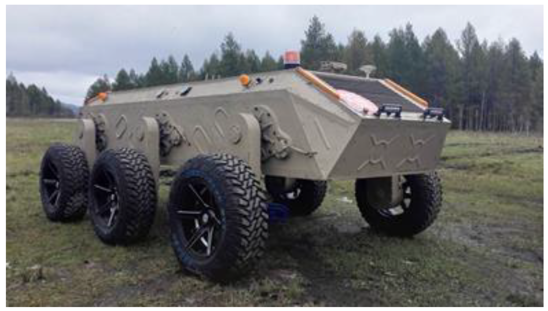
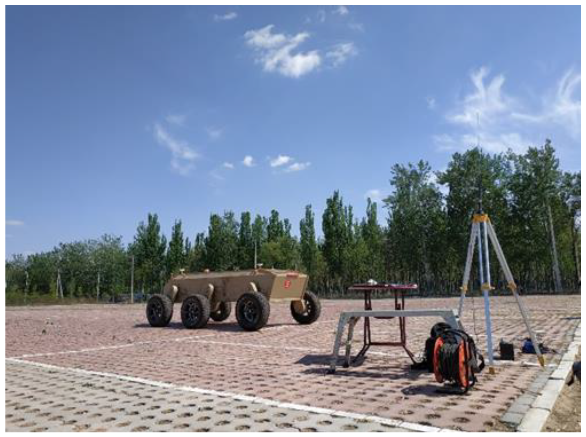
In this section, an experiment test is set up to verify the proposed estimation algorithm in this paper. The experiment platform is designed by our library, and the sensors set up on the vehicle are introduced. The experiment platform is a six-wheel drive skid-steered wheeled UGV with articulated suspension. The platform is shown in Figure 10.

5.1. Experimental Platform Introduction

The platform mainly includes the articulated suspension system and wheel drive system. The articulated suspension system includes six sets of longitudinal rocker arms that can rotate 360 degrees controlled by the adjustment mechanism using planetary deceleration combined with an electromagnetic brake. The drive system of the platform includes two sets of drive motors and corresponding transmission devices. Two driving motors are installed on the two sides of the vehicle body to drive the three wheels on the same side by transmission. The torque is given by the motor controller and the speed is given by the encoder. The motion speed of the wheel on the same side is the same because of the mechanical structure of the drive system. This scheme can greatly improve the power and suspension performance of the vehicle while reducing the weight of the vehicle and greatly improving the off-road performance. The essential parameters of the platform are shown in

Table 1. Essential parameters of the platform.

Parameters	Symbols	Value
Vehicle mass	m (kg)	3000
Length of the vehicle	L (m)	4.7
Width of the vehicle	B (m)	2.060
Length of the arm	l (m)	0.7
Distance between 1st and 2nd axes	a (m)	1.836
Distance between 2nd and 3rd axes	b (m)	1.036
Distance between 2nd and CM	x (m)	0.244
Distance between each axes	c (m)	1.400
Height of CM	h (m)	0.600
Rotational inertia round z-axis	Iz (kg·m2)	6390
Transmission rate	i	27.13
Width of the tire	Bw (m)	0.210
Radius of the tire	R (m)	0.375

.

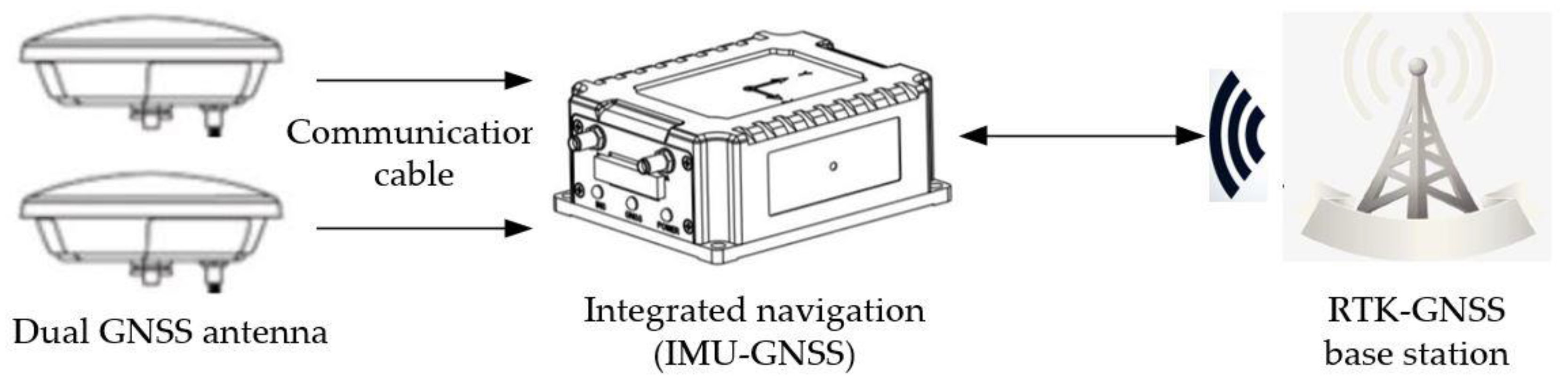
The sensors installed on the UGV include an integrated navigation system, a binocular camera, an 8-line LIDAR, and a 32-line LIDAR. The integrated navigation system includes the IMU, GNSS, and dual antennas corresponding to the GNSS. The IMU is located on the geometric center to provide the acceleration and rotation rate on the three axes. According to the assumption that the center of mass is located on the geometric center, the location of the IMU is to decrease the bias caused by the installation site. The dual antenna is located on the axle wire of the UGV. The RTK-GNSS can provide accurate longitude and lateral velocity, position, and direction information. The accuracy of the RTK-GNSS is shown in

Table 2. Accuracy of the RTK-GNSS.

Parameters	Value
Horizontal position accuracy	0.01 m
Vertical position accuracy	0.02 m
Speed accuracy	0.007 m/s

.

The binocular camera and the 8-line LIDAR are located on the front of the vehicle body to gather the environmental information. The 32-line LIDAR is located on the top of the vehicle body to detect the obstruction. In this study, the environmental information obtained from the camera and the LIDAR is not used. The sensors applied in the estimation algorithm include the IMU, RTK-GNSS, and the encoder of the motor. The experimental platform and the RTK-GNSS base station are shown in Figure 11. The diagram of the measuring system is shown in Figure 12.

5.2. Experimental Verification of the Tire Parameters Estimation Algorithm

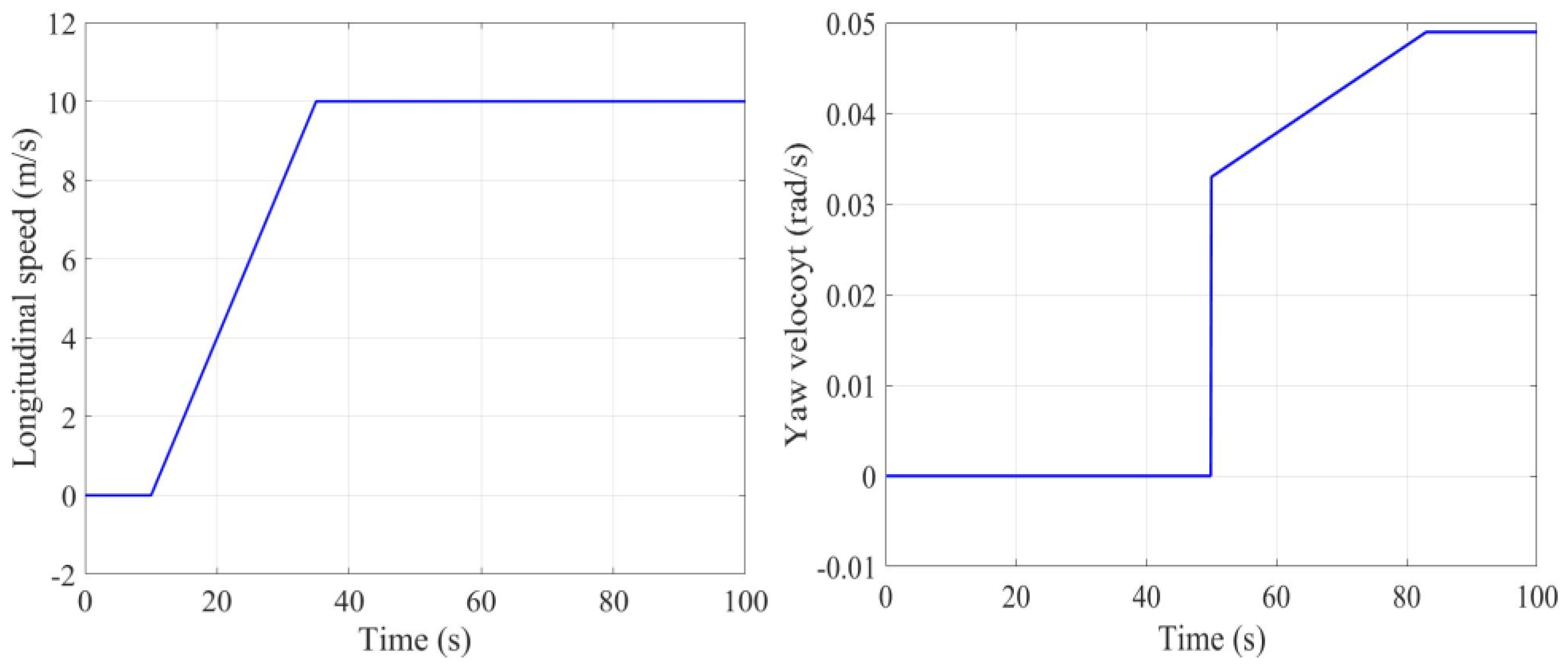
In this section, the simulation condition is set in the co-simulation platform of TruckSim and Simulink. The motion of the vehicle simulation model in TruckSim is shown in Figure 13. From 10 s, the vehicle starts to accelerate uniformly straight to 10 m/s, after which the speed remains stable. From 50 s, the vehicle begins to turn, and reaches the steady-state steering at 83 s, with a yaw rate of about 0.05 rad/s.

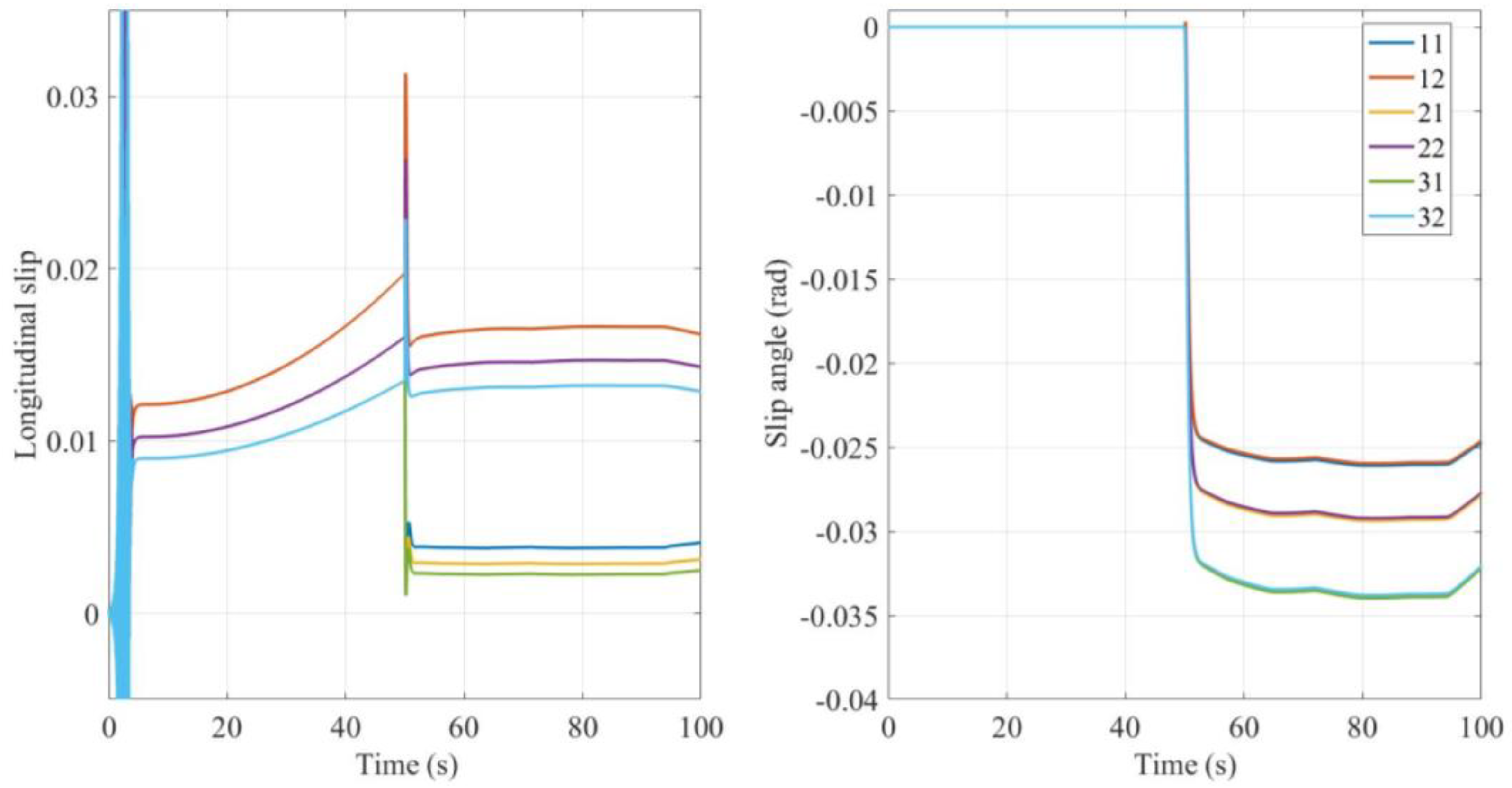
The longitudinal slip ratio and cornering angle of the tire under simulation driving conditions are shown in Figure 14. Due to the instability of the dynamic model of the simulation software itself, a large vibration is generated in the first few seconds. Therefore, the verification of the estimation algorithm will begin after the vehicle is stable. The object estimated in this paper is the relevant parameters of the Brush nonlinear tire model used in Section 3.

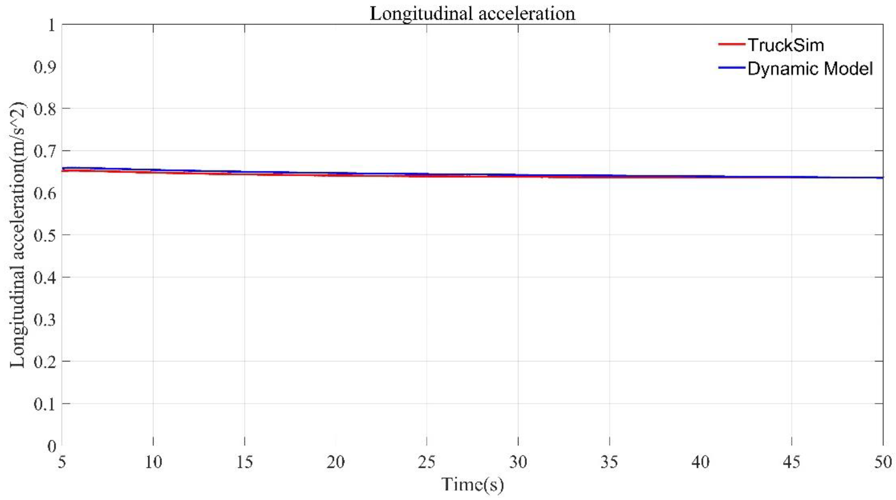
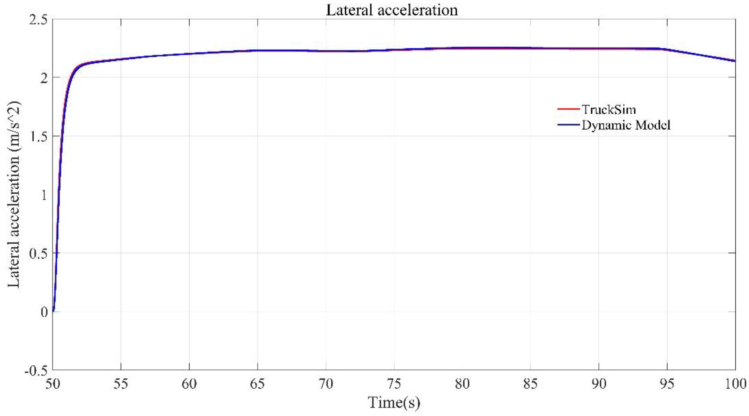
The tire parameter estimation results obtained by the offline estimation algorithm are input into the Brush nonlinear tire model used in Section 3. On this basis, the 3-DOF dynamic model of the skid-steered wheeled UGV established in chapter 3 is used to calculate the dynamic model output of the tire model obtained by the estimation algorithm under the current working condition. Then, the output is compared with the relevant motion state of the TruckSim model output to verify the accuracy of the estimation algorithm applied in this paper. The comparison of the lateral and longitudinal acceleration output by the nonlinear dynamic model of the longitudinal stiffness and cornering stiffness of the tire obtained by the estimation algorithm and the longitudinal and lateral acceleration output by TruckSim are shown in Figure 15 and Figure 16 respectively, respectively.

Since the relevant parameters of the tire can be obtained directly in TruckSim, the comparison between the lateral and longitudinal stiffness of the tire obtained by the estimation algorithm under TruckSim simulation conditions and the actual tire model parameters in the TruckSim model is shown in

Table 3. Tire parameter estimation results and error analysis.

	True Value	Estimation Results	Absolute Error	Relative Error
Longitudinal stiffness (N)	33,507	33,141	366	0.69%
Cornering Stiffness (N/rad)	41,020	39,572	1448	3.37%

. It can be seen that the tire parameter estimation algorithm used in this paper can accurately estimate the longitudinal and cornering stiffness of the tire.

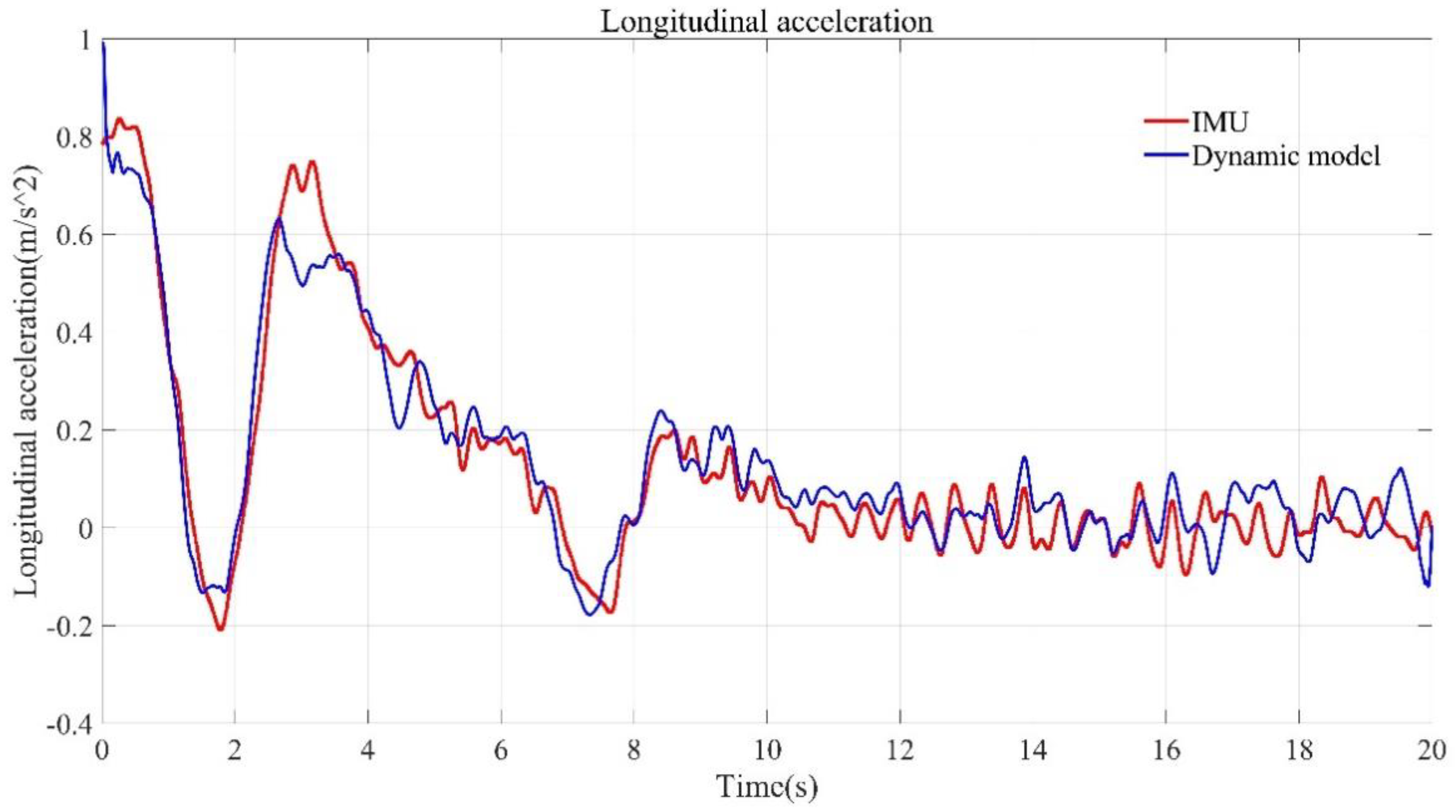
Then, the real vehicle test data are used to verify the tire parameter estimation algorithm. Based on the real vehicle test data, the lateral and longitudinal vehicle speeds measured by RTK-GPS are applied to calculate the longitudinal slip rate and sideslip angle of the tire. The vehicle tire parameters estimated by the algorithm proposed in this paper are applied to calculate the tire force. The nonlinear dynamic model is applied to calculate the lateral and longitudinal acceleration of the vehicle. The final estimation results are: tire longitudinal stiffness, 16,270 N; cornering stiffness, 13,211 N/rad. The comparison between the output results of the vehicle dynamics model and the real vehicle motion state is shown in Figure 17, Figure 18, Figure 19 and Figure 20.

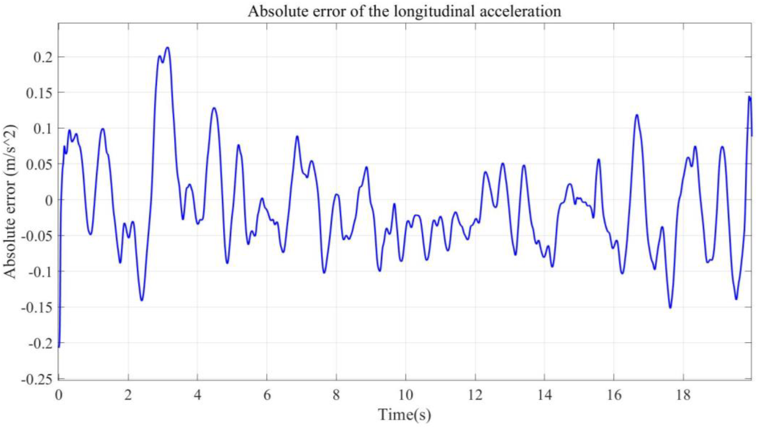
The comparison between the longitudinal acceleration results from the nonlinear dynamic model using the longitudinal and cornering stiffness obtained by the estimation algorithm and the real vehicle test under the same driving conditions is shown in Figure 17. The absolute error of the longitudinal acceleration from the nonlinear dynamic model using the longitudinal and cornering stiffness obtained by the estimation algorithm and the real vehicle test under the same working condition is shown in Figure 18. The standard deviation of the output of the dynamic model is ${\sigma }_{ay}=0.0662\hspace{0.17em}{\mathrm{m}/\mathrm{s}}^2$, and the cumulative velocity of the longitudinal acceleration error in 20 s is $v_{y\_err}=-0.1879\hspace{0.17em}\mathrm{m}/\mathrm{s}$.

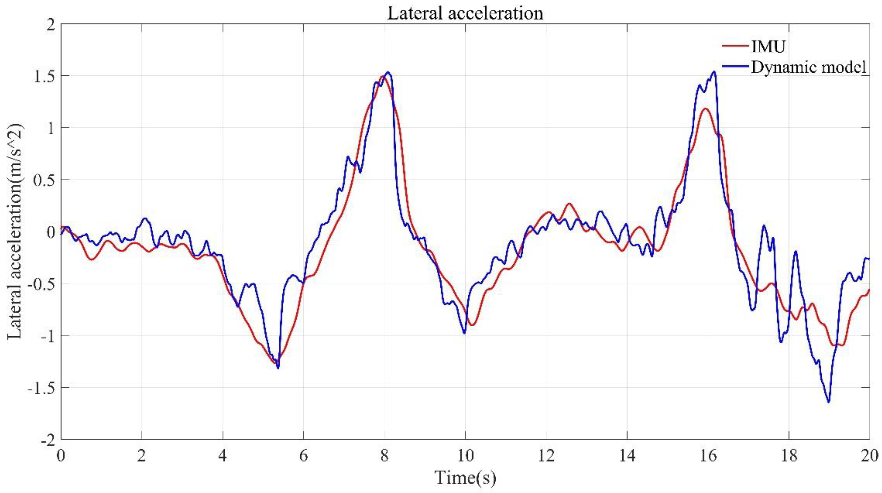
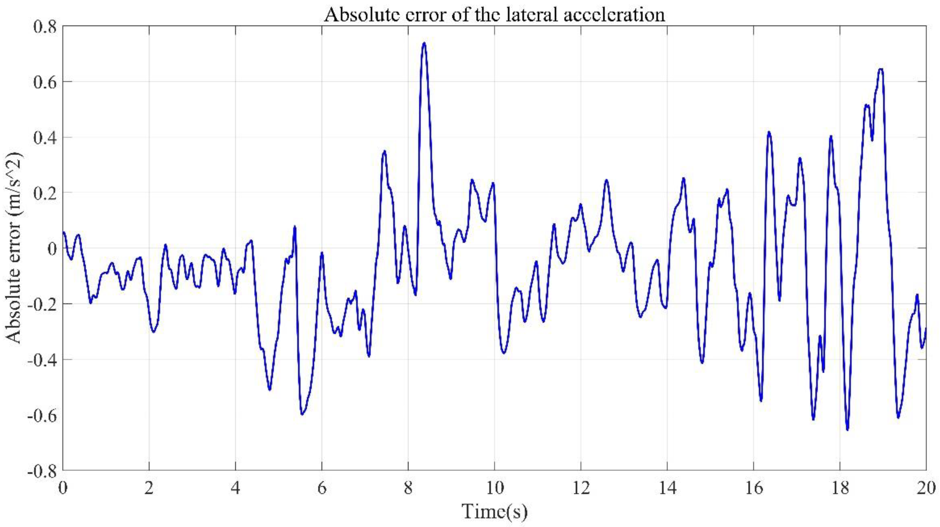
The comparison between the lateral acceleration results from the nonlinear dynamic model using the longitudinal and cornering stiffness obtained by the estimation algorithm and the real vehicle test under the same driving conditions is shown in Figure 19. The absolute error of the lateral acceleration from the nonlinear dynamic model using the longitudinal and cornering stiffness obtained by the estimation algorithm and the real vehicle test under the same working condition is shown in Figure 20. The standard deviation of the output of the dynamic model is ${\sigma }_{ay}=0.2469\hspace{0.17em}{\mathrm{m}/\mathrm{s}}^2$, and the cumulative velocity of the longitudinal acceleration error in 20 s is $v_{y\_err}=-1.2969\hspace{0.17em}\mathrm{m}/\mathrm{s}$. It can be seen that the lateral and longitudinal acceleration of the vehicle obtained from the tire model estimation results is in good agreement with the real vehicle test. It is also noted that the accuracy of the model output value of the longitudinal acceleration is relatively higher than that of the model output value of the lateral acceleration.

5.3. Experimental Verification of the Road Adhesion Coefficient Estimation Algorithm

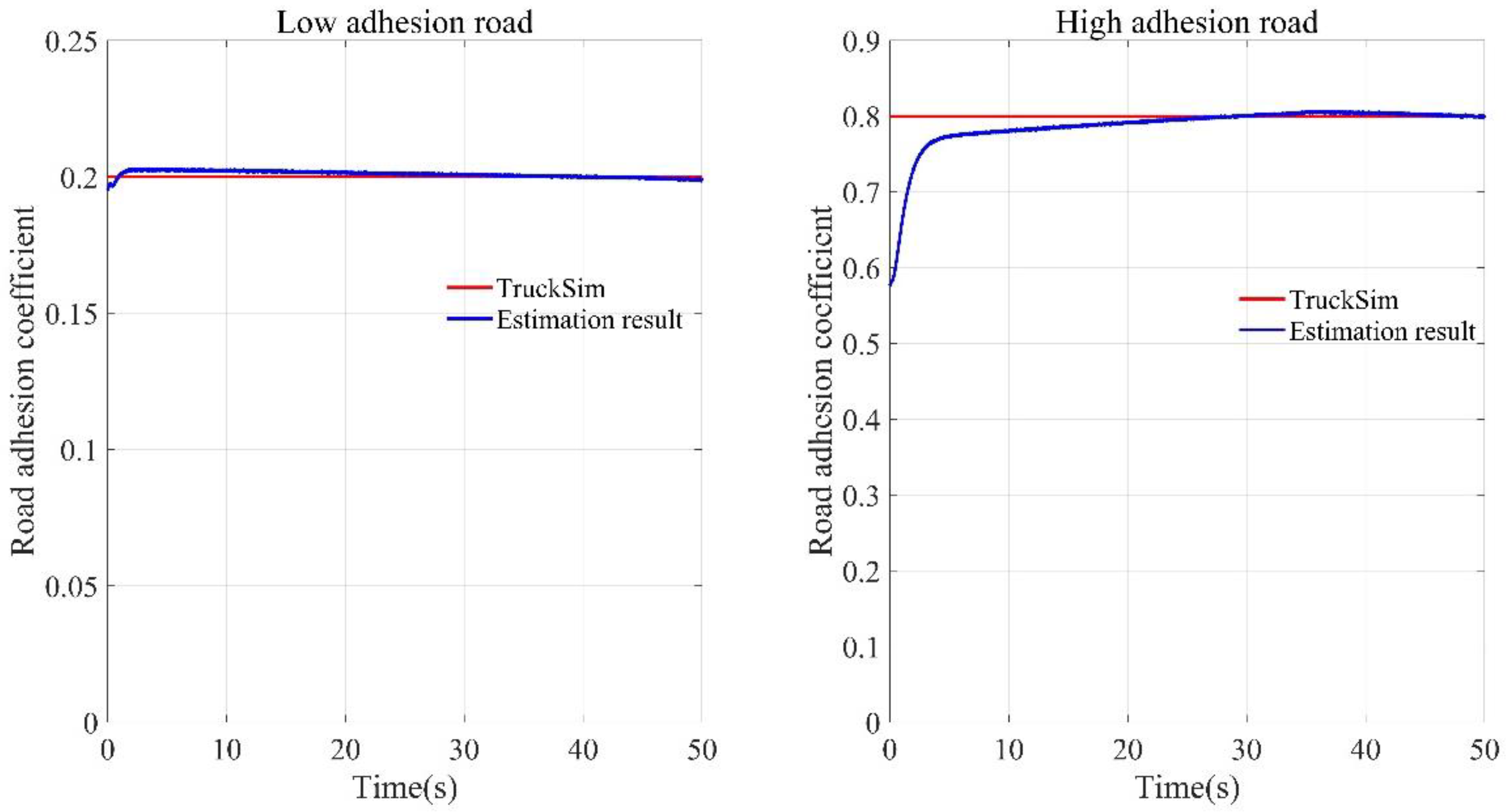
According to the road adhesion coefficient estimation algorithm proposed in Section 4.2, the straight-line driving conditions are selected to identify road parameters in this study. Two kinds of roads are chosen to verify the road adhesion coefficient estimation algorithm. The simulation platform is TruckSim and Simulink co-simulation.

The road adhesion coefficient estimation results are shown in Figure 21. Whether it is a low-adhesion road or a high-adhesion road, the road adhesion coefficient estimation algorithm for the skid-steered wheeled UGV proposed in this paper can estimate the current road adhesion coefficient quickly and accurately.

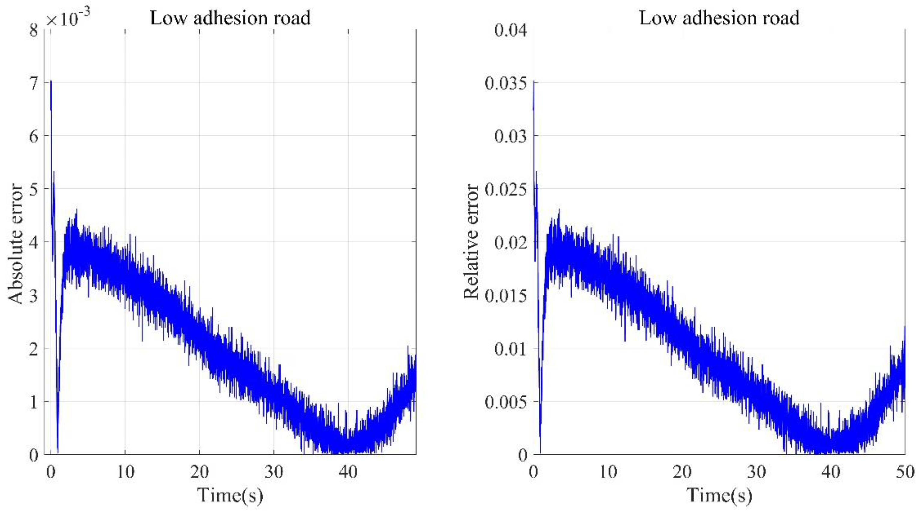
The error analysis of the estimation algorithm under a low-adhesion road is shown in Figure 22, including the absolute error and the relative error. For the low-adhesion road, the real value of the road adhesion coefficient is set to 0.2. Since the initial value is set to be close to the true value, the estimation result can quickly approach the real value of the road adhesion coefficient, and the relative error of the estimation result is quickly reduced to below 2%. It can be verified that the estimation result of the algorithm under a low-adhesion road can meet the requirements both in convergence speed and error.

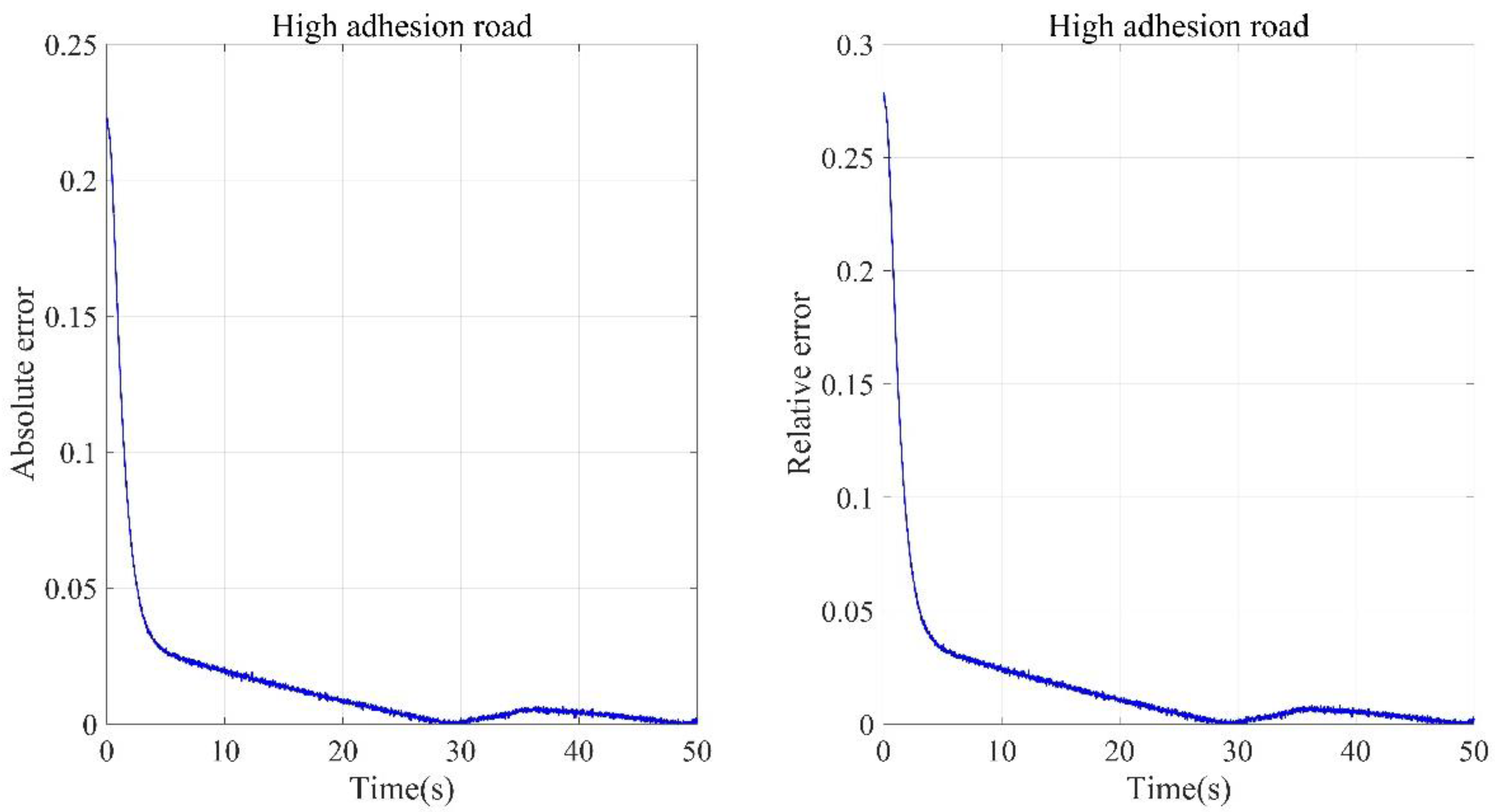
The error analysis of the estimation results under a high-adhesion road is shown in Figure 23. For high-adhesion roads, the real value of the road adhesion coefficient is set to 0.8. From the error analysis diagram, it can be seen that under the high-adhesion road, the relative error of the road adhesion coefficient is reduced to less than 5% at about 2 s, and then maintained within 5%. Although the convergence speed and estimation accuracy slightly are worse than the low-adhesion road, they still have a high accuracy to meet system requirements.

6. Conclusions

In this paper, a complete system estimation method of vehicle tire parameters and tire–road adhesion coefficient is established for a skid-steered wheeled vehicle considering the dynamic characteristics, which provide parameter support for vehicle motion planning and control systems.

Based on the dynamic characteristics of the skid-steered wheeled vehicle and considering the power steering characteristics, an offline tire parameter estimation algorithm of the skid-steered wheeled vehicle based on the PSO algorithm is established, and the PSO algorithm is improved by using the adaptive weight method to improve its convergence.

Based on the dynamic characteristics of the skid-steered wheeled vehicle and the Brush nonlinear tire model, according to the Burckhardt road adhesion coefficient formula, a road adhesion coefficient estimation algorithm based on the EFRLS algorithm is designed to estimate the tire–road adhesion coefficient in real-time.

The effectiveness of the estimation algorithms proposed in this paper is verified by TruckSim simulation test and real vehicle test.

References

Zhang, X.; Pei, W.; Yin, X.; Yuan, S. An observation algorithm for key motion states of skid-steered wheeled unmanned vehicle. Proc. Inst. Mech. Eng. Part D J. Automob. Eng.2021. [Google Scholar] [CrossRef]
Ni, J.; Hu, J.; Li, X. Dynamic modelling, validation and handling performance analysis of a skid-steered vehicle. Proc. Inst. Mech. Eng. Part D J. Automob. Eng.2016, 230, 514–526. [Google Scholar] [CrossRef]
Chen, H.; Zhang, Y. An overview of research on military unmanned ground vehicles. Acta Armamentarii2014, 35, 1696–1706. [Google Scholar] [CrossRef]
Gao, X.; Li, X.; Liu, Q.; Li, Z.; Yang, F.; Luan, T. Multi-Agent Decision-Making Modes in Uncertain Interactive Traffic Scenarios via Graph Convolution-Based Deep Reinforcement Learning. Sensors2022, 22, 4586. [Google Scholar] [CrossRef] [PubMed]
Liu, Q.; Li, X.; Yuan, S.; Li, Z. Decision-Making Technology for Autonomous Vehicles: Learning-Based Methods, Applications and Future Outlook. In Proceedings of the 24th IEEE International Conference on Intelligent Transportation Systems, Indianapolis, IN, USA, 19–22 September 2021. [Google Scholar]
Lian, Y.F.; Zhao, Y.; Hu, L.L.; Tian, Y.T. Cornering stiffness and sideslip angle estimation based on simplified lateral dynamic models for four-in-wheel-motor-driven electric vehicles with lateral tire force information. Int. J. Automot. Technol.2015, 16, 669–683. [Google Scholar] [CrossRef]
Lee, S.; Nakano, K.; Ohori, M. On-board identification of tyre cornering stiffness using dual Kalman filter and GPS. Veh. Syst. Dyn.2015, 53, 437–448. [Google Scholar] [CrossRef]
Wang, Y.; Geng, K.; Xu, L.; Ren, Y.; Dong, H.; Yin, G. Estimation of Sideslip Angle and Tire Cornering Stiffness Using Fuzzy Adaptive Robust Cubature Kalman Filter. IEEE Trans. Syst. Man Cybern. Syst.2022, 52, 1451–1462. [Google Scholar] [CrossRef]
Berntorp, K.; Di Cairano, S. Tire-Stiffness and Vehicle-State Estimation Based on Noise-Adaptive Particle Filtering. IEEE Trans. Control Syst. Technol.2019, 27, 1100–1114. [Google Scholar] [CrossRef]
Wang, R.; Wang, J. Tire–road friction coefficient and tire cornering stiffness estimation based on longitudinal tire force difference generation. Control Eng. Pract.2013, 21, 65–75. [Google Scholar] [CrossRef]
Sierra, C.; Tseng, E.; Jain, A.; Peng, H. Cornering stiffness estimation based on vehicle lateral dynamics. Veh. Syst. Dyn.2006, 44 (Suppl. 1), 24–38. [Google Scholar] [CrossRef]
Pereira, C.; da Costa Neto, R.; Loiola, B. Cornering stiffness estimation using Levenberg–Marquardt approach. Inverse Probl. Sci. Eng.2021, 29, 2207–2238. [Google Scholar] [CrossRef]
Guo, H. Study on Nonlinear Observer Method for Vehicle Velocity Estimation. Ph.D. Thesis, Jilin University, Changchun, China, 2010. [Google Scholar]
El Tannoury, C.; Plestan, F.; Moussaoui, S.; Gil, G.P. A variable structure observer for an on-line estimation of a tyre rolling resistance and effective radius. In Proceedings of the 12th International Workshop on Variable Structure Systems, Mumbai, India, 12–14 January 2012. [Google Scholar]
Han, Y.; Lu, Y.; Liu, J.; Zhang, J. Research on Tire/Road Peak Friction Coefficient Estimation Considering Effective Contact Characteristics between Tire and Three-Dimensional Road Surface. Machines2022, 10, 614. [Google Scholar] [CrossRef]
Yu, Z.; Zuo, J.; Zhang, L. A summary on the development status of tire-road friction coefficient estimation techniques. Automot. Eng.2006, 28, 546–549. [Google Scholar]
Liu, C.; Peng, H. Road friction coefficient estimation for vehicle path prediction. Veh. Syst. Dyn.1996, 25, 413–425. [Google Scholar] [CrossRef]
Wang, J.; Alexander, L.; Rajamani, R. Friction estimation on highway vehicles using longitudinal measurements. J. Dyn. Syst. Meas. Control2004, 126, 265–275. [Google Scholar] [CrossRef]
Shim, T.; Margolis, D. Using µ feedforward for vehicle stability enhancement. Veh. Syst. Dyn.2001, 35, 103–119. [Google Scholar] [CrossRef]
Ghandour, R.; Victorino, A.; Doumiati, M.; Charara, A. Tire/road friction coefficient estimation applied to road safety. In Proceedings of the 18th Mediterranean Conference on Control and Automation MED’10, Marrakech, Morocco, 23–25 June 2010. [Google Scholar]
Villagra, J.; D’Andréa-Novel, B.; Fliess, M.; Mounier, H. A diagnosis-based approach for tire–road forces and maximum friction estimation. Control. Eng. Pract.2011, 19, 174–184. [Google Scholar] [CrossRef] [Green Version]
Patra, N.; Datta, K. Observer based road-tire friction estimation for slip control of braking system. Procedia Eng.2012, 38, 1566–1574. [Google Scholar] [CrossRef] [Green Version]
Zhang, X.; Yuan, S.; Yin, X.; Li, X.; Qu, X.; Liu, Q. Estimation of Skid-Steered Wheeled Vehicle States Using STUKF with Adaptive Noise Adjustment. Appl. Sci.2021, 11, 10391. [Google Scholar] [CrossRef]
Riehm, P.; Unrau, H.-J.; Gauterin, F.; Torbrügge, S.; Wies, B. 3D brush model to predict longitudinal tyre characteristics. Veh. Syst. Dyn.2019, 57, 17–43. [Google Scholar] [CrossRef]
Zhuo, G.; Jin, W.; Zhang, F. Parameter Identification of Tire Model Based on Improved Particle Swarm Optimization Algorithm. SAE Int.2015, 1, 1586. [Google Scholar] [CrossRef]
Burckhardt, M. Vehicle Chassis Technology-Wheel Sub System; Vogel-Verlag: Wurtzburg, Germany, 1993; pp. 18–33. [Google Scholar]
Zhu, Y. Efficient recursive state estimator for dynamic systems without knowledge of noise covariances. IEEE Trans. Aerosp. Electron. Syst.1999, 35, 102–114. [Google Scholar] [CrossRef]
Figure 1.
Kinematics diagram of the skid-steered wheeled UGV.
Figure 2.
Force analysis for 3-DOF dynamics model.
Zhu, Y.; Li, X.; Zhang, X.; Li, S.; Liu, Q.; Yuan, S.