Study on the Control Algorithm of Automatic Emergency Braking System (AEBS) for Commercial Vehicle Based on Identification of Driving Condition

Abstract

Automatic emergency braking systems (AEBS) significantly improve the active safety performance of commercial vehicles, but their effectiveness is affected by the vehicle’s driving conditions, which mainly include the vehicle load and road conditions. In order to improve the adaptability of the AEBS, an AEBS control strategy with adaptive driving conditions was proposed and validated using a simulation and experimentation. This AEBS control strategy was designed based on an estimation of the vehicle mass, the center of gravity position, road grade, and the tire-road friction coefficient. In the simulation and experimental verification, the braking deceleration and braking distance under different driving conditions were compared. The results show that the AEBS control strategy proposed in this paper can avoid collisions in all test scenarios and maintain a parking spacing of approximately 5 m. In an extreme test scenario with a full load and low tire–road friction, as compared with the fixed threshold control strategy, the warning can be issued 0.2 s earlier and the maximum intensity braking can be carried out 0.5 s earlier.

1. Introduction

Vehicle braking has long been a hot issue in the field of dynamics. Various scholars are concerned about energy consumption during vehicle braking and have conducted in-depth research on braking energy recovery [1,2]. There are also researchers who focus on the safety aspects of vehicle braking. With the increase in vehicle rear-end accidents in recent years [3], automatic emergency braking systems for vehicle safety are becoming increasingly important. The AEBS can prevent rear-end collisions or mitigate collision injuries by providing early warnings and braking automatically when necessary [4]. Unlike passenger cars, commercial vehicles have to work in complex and variable driving conditions, with large mass variations and a high center of gravity [5]. Therefore, when developing an automatic emergency braking system for commercial vehicles, it is necessary to identify the driving conditions of the vehicle in order to improve the robustness of the control strategy.

The AEBS can be generally divided into a sensing layer, a decision layer, and an actuation layer [6]. The parameters acquired by the sensing layer can be divided into three categories: the relative motion parameters of the target vehicle and the host vehicle, the load parameters of the host vehicle, and the road parameters. The relative motion parameters include relative speed, relative distance, and relative acceleration, which can be obtained directly by radar or camera sensors [7]. The load parameters of the host vehicle mainly refer to the mass and center of gravity position. The load parameter estimation method based on vehicle sensors requires the additional installation of corresponding sensors [8], which increases the vehicle upgrade cost and the complexity of the system [9]. In addition, there are road bumps, suspension deformation, and other factors in the process of vehicle driving, and the accuracy of parameter acquisition is poor. The load parameter estimation method based on the vehicle dynamics model does not require additional hardware for calculations and is therefore more widely used [10].

The road parameters include the road grade and the tire-road friction coefficient. These two types of parameters cannot be directly obtained by the cost limitation of the sensors, so they need to be estimated [6]. The instantaneity and accuracy of the parameters acquired by the sensing layer are crucial to the control decision [11].

The estimation methods of the tire–road friction coefficient are divided into cause-based and effect-based estimation methods [12], in which cause-based estimation methods require the direct measurement of the tire-road friction coefficient with sensors or indirect calculations by measuring the effect of friction [13,14]. Cause-based estimation methods are predictive in estimating the road surface, but the sensors are sensitive to environmental changes and are less robust. Effect-based estimation methods estimate the tire-road friction coefficient by analyzing the response of the vehicle as a result of pavement changes. This type of method does not generally require additional sensors and does not require an ideal working environment [15,16,17].

The use of known vehicle dynamics and kinematic information to determine the current driving conditions of the vehicle without increasing the complexity of the system plays a key role in improving control effectiveness.

The decision layer of the AEBS for commercial vehicles makes early warning and braking decisions based on various types of information obtained from the sensing layer and sends a brake request to the actuation layer [18]. If the AEBS acts too early, it affects the normal operation of the driver and makes the driver distrust the AEBS, while intervening too late may lead to safety problems [19]; therefore, the rationality of the AEBS decision directly affects the driving experience and the synergistic control effect of safety during braking. The AEBS control strategy can generally determine whether the system needs to perform early warning or emergency braking based on a distance scale or time scale [20,21]. The relative distance-based discrimination method uses the relative distance as an indicator to measure the level of danger, and compares this with the threshold value to guide the AEBS for collision avoidance operations, e.g., warning and emergency braking [22,23]. This method is simple to implement, but the preset threshold is mainly determined by parameters such as the speed of the host vehicle, the relative speed of the target vehicle, and the maximum braking deceleration of the host vehicle [24]. However, real-world driving scenarios are more complex and variable, so other parameters that have an impact on the braking distance need to be introduced into the control strategy. Another discrimination method using the time scale is the time to collision (TTC), which is an indicator of the hazard status [18]. In the driving process, the driver has a more intuitive feeling of the remaining collision occurrence time [25,26], but the preset TTC value does not have scenario adaptability. Therefore, an AEBS control strategy that is based on the actual driving condition of the vehicle and that combines the safe distance and TTC is the key to ensuring both a good driving experience and braking safety.

Compared to the current work, this paper proposes an AEBS control strategy that adjusts the decision parameters in real time according to the actual driving conditions of the vehicle. The traditional AEBS sensing layer function was optimized by considering vehicle mass and road conditions, and the vehicle driving information is fully utilized without changing the system architecture. The estimation module of the load state and road conditions was added and the dynamics constraints of the actual driving condition of the vehicle were constructed. These parameters and constraints can be applied to the real-time adjustment of the control parameters. An AEBS control strategy with a driving condition adaptation is proposed, which can formulate real-time solutions for AEBS strategy control parameters under longitudinal dynamics constraints in different driving conditions, ensuring the adaptability and control robustness of the AEBS. Finally, the developed algorithm was validated in field tests for various driving conditions. The results show that the AEBS control strategy proposed in this paper can avoid collisions in all test scenarios and maintain a parking spacing of approximately 5 m. In the extreme test scenario with a full load and low tire–road friction, as compared with the fixed threshold control strategy, the warning can be issued 0.2 s earlier and the maximum intensity braking can be carried out 0.5 s earlier.

2. AEBS Control Strategy with Driving Condition Identification

2.1. Control Strategy Framework and Simulation Settings

In this paper, a control strategy based on the vehicle driving conditions is proposed. The AEBS framework is shown in Figure 1. The control strategy is divided into a sensing layer and a decision layer. The function of the sensing layer is to obtain driving information in relation to the target vehicle and estimate the driving condition of the host vehicle. The function of the decision layer includes braking deceleration decisions and braking force distribution. The control strategy outputs the desired braking force of each axis to the vehicle model and completes the closed-loop control.

To validate the proposed estimation method, a simulation platform was constructed using Matlab Simulink (MathWorks, United States of America) and TruckSim(Mechanical Simulation Corporation, United States of America). Matlab Simulink was used to build the estimation method for the vehicle load state and road conditions. The vehicle dynamics model in TruckSim is used to accurately calculate the vehicle motion state and parameters such as the vehicle load, road grade, and the tire-road friction coefficient. Moreover, the relative motion state of the target vehicle and host vehicle are set in TruckSim, and the relative motion information is transferred to the control strategy. The architecture of the proposed co-simulation platform is shown in Figure 2.

The vehicle in this paper is a two-axle van, and the vehicle parameters are shown in

Table 1. Vehicle parameters.

Items	Values	Items	Values
Mass of vehicle fully loaded (kg)	17,000	Tire type	275/80R22.5
Vehicle weight (kg)	6300	Vehicle length (mm)	9000
Wheelbase (mm)	5300	Vehicle width (mm)	2550
Axle track(mm)	1943/1860	Vehicle height (mm)	3500

.

2.2. Sensing Layer

The inputs to the sensing layer are divided into two categories. One is the relative driving information from the radar, including relative velocity, relative distance, and relative acceleration, which can be directly transferred to the decision layer. The second is the vehicle’s driving information, such as vehicle speed, transmission ratio, and engine torque, which is used to estimate the vehicle load state, the mass center location, the road grade, and the tire-road friction coefficient.

2.2.1. Vehicle Load State and Road Grade Estimation

Since the vehicle system is complex, each component affects each other, resulting in a significant coupling phenomenon between the vehicle system’s state parameters. The vehicle mass and road grade are a set of mutually coupled quantities, so these two quantities are estimated successively. The schematic diagram of the vehicle load state and grade estimation method is shown in Figure 3. First, we need to determine whether the vehicle is in the starting state, and when the vehicle is in the starting state, we perform an estimation of the mass and use the estimation result in the estimation of the road slope.

The vehicle mass only generally changes in the starting condition, and can be treated as a constant during driving, so the vehicle mass can be estimated based on the engine output torque and wheel speed. The vehicle ESC (electronic stability control) system is equipped with an acceleration sensor, which can be used to measure the static inclination of the vehicle.

The flow of the vehicle start state discernment is shown in Figure 4. When the engine is in the idle scenario, the transmission is in neutral position, and the vehicle velocity is 0 km/h, it can be determined that the vehicle is currently in the normal stop state. The stop state flag bit is expressed as $F_{stop}=1$; after a period of time (such as 2 s), if the vehicle velocity exceeds a certain value and no braking signal appears, the vehicle is considered to be in the starting acceleration state. The transmission cannot be shifted, and the wheels do not slip during the process.

After determining that the vehicle is in the starting state, the vehicle mass is estimated by applying the least squares method based on the vehicle longitudinal dynamics equation, as shown in Equation (1).

$$\frac{T_{tq}{i}_0{i}_g{\eta }_t}{r}=mg\sin \beta +\frac{1}{2}{C}_{D}A\rho v^2+mgf\cos \beta +\delta m\dot{v}$$

(1)

where $m$ denotes the vehicle mass, $v$ denotes the vehicle longitudinal speed, $I_w$ denotes the rotating inertia of the wheels, $I_f$ denotes the rotating inertia of the flywheel, $I_0$ denotes the final drive gear ratio, $i_g$ denotes the vehicle transmission ratio, $T_{tq}$ denotes the engine torque, ${\eta }_t$ denotes the transmission efficiency, $r$ denotes the wheel rolling radius, $C_D$ denotes the wind resistance coefficient, $A$ denotes the windward area, $\rho$ denotes the air density, $f$ denotes the road rolling resistance coefficient, $\beta$ denotes the road grade, and $\delta =1+\frac{1}{m}\frac{{\displaystyle \sum I_w}}{r^2}+\frac{1}{m}\frac{I_f{i}_g^2{i}_0^2{\eta }_t}{r^2}$ denotes the rotary mass coefficient.

The vehicle longitudinal dynamics equations are transformed into a least-squares format as follows:

$$\mathrm{y}={\varphi }^T\theta$$

(2)

where

$$\mathrm{y}=\dot{v}$$

(3)

Thus,

$$\dot{v}=\frac{1}{m}(\frac{T_{tq}{i}_0{i}_g{\eta }_t-I\cdot \dot{\omega }}{r}-\frac{1}{2}{C}_{D}A\rho v^2)-\frac{g}{\cos \alpha }\sin (\beta +\alpha )$$

(4)

$$\varphi =\left[\begin{array}{c}\frac{T_{tq}{i}_0{i}_g{\eta }_t-I\cdot \dot{\omega }}{r}-\frac{1}{2}{C}_{D}A\rho v^2\\ -\frac{g}{\cos \alpha }\end{array}\right]$$

(5)

$$\theta =\left[\begin{array}{c}\frac{1}{m}\\ \sin (\alpha +\beta )\end{array}\right]$$

(6)

The mass of the vehicle was estimated on a horizontal road unladen and with a full load, respectively. In the simulation, the vehicle accelerated straight at an initial speed of 0 km/h on a good road surface. The results of the vehicle mass estimation are shown in Figure 5 and

Table 2. Summary of vehicle mass estimation results.

	True Value(kg)	Estimated Value(kg)	Relative Error
Unladen	6300	6417	1.85%
Full load	17,000	16,420	3.41%

.

As can be seen in Figure 5 and Table 2, the least-squares mass estimation method based on the starting state of the vehicle can be used to estimate the vehicle mass, and the estimation results are close to the real values. The absolute value of the difference between the steady-state estimated value and the true value was divided by the true value, as in the error calculation method. The method converged quickly and the steady-state error between the estimated value and the actual value was shown to be within 3.5%. The estimation results were applied to the subsequent road grade estimation in real time and to the control strategy.

Road grade simulations were performed under varying road grades and a fixed vehicle gear ratio. The estimation results are shown in Figure 6 and

Table 3. Road grade estimation results.

Real Value of Road Grade (%)	Estimated Value of Road Grade (%)	Absolute Error
10%	9.69%	0.31%
0%	0.15%	0.15%
−10%	−9.85%	0.15%

.

As shown in Figure 6 and Table 3, the method proposed in this paper can estimate the real-time change in road grade, the convergence speed of this method is fast, and the absolute error is within 0.35%.

2.2.2. Vehicle Mass Center Location Estimation

The load mass of commercial vehicles varies considerably, and the load distribution is unpredictable. Thus, it is necessary to calculate the load transfer between the front and rear axles according to the center of gravity position in order to ensure a reasonable braking force distribution. Most commercial vehicles are now equipped with air spring suspension. The pressure sensor in the air spring of the air suspension can measure the air pressure value, and the load value $G_r$ of the rear axle of the commercial vehicle can be estimated based on the air pressure.

When the vehicle is driven on a horizontal road, the ground normal reaction force can be given by:

$$F_{zf}=mg\cos \beta \frac{b}{L}+(mg\sin \beta +m\dot{v})\frac{h_g}{L}-\frac{1}{2}{C}_{D}A\rho v^2\frac{h_a}{L}$$

(7)

$$F_{zr}=mg\cos \beta -mg\cos \beta \frac{b}{L}+(mg\sin \beta +m\dot{v})\frac{h_g}{L}-\frac{1}{2}{C}_{D}A\rho v^2\frac{h_a}{L}$$

(8)

where $L$ is the wheelbase, $F_{zf}$ and $F_{zr}$ are the vertical load of the front and rear wheels, respectively, $a$ and $b$ are the distances from the center of mass to the front and rear axles, respectively, $h_a$ is the distance from the point of action of the air resistance and other effects to the ground, and $h_g$ is the distance from the center of gravity to the ground.

In this paper, the center of gravity position is estimated using the CKF method. The parameters to be estimated are the distance b from the center of mass to the back axis and the height $h_g$ of the center of mass.

Equations (7) and (8) were transformed into the standard form for CKF filtering. The state vector, observation vector, and system expression of the CKF filtering algorithm are as follows:

$$x={[\begin{array}{cc}b& h_g\end{array}]}^T$$

(9)

$$z=\left[\begin{array}{c}{F}_{zf}+\frac{1}{2}{C}_{D}A\rho v^2\frac{h_a}{L}\\ F_{zr}-mg\cos \beta -\frac{1}{2}{C}_{D}A\rho v^2\frac{h_a}{L}\end{array}\right]$$

(10)

$$x_k=x_{k-1}+w(k)$$

(11)

$$z_k=\left[\begin{array}{cc}\frac{mg\cos \beta }{L}& -\frac{mg\sin \beta +m{\dot{v}}_x}{L}\\ -\frac{mg\cos \beta }{L}& \frac{mg\sin \beta +m{\dot{v}}_x}{L}\end{array}\right]x_k+v_k$$

(12)

where $w(k)\sim N(0,Q_k)$ is the system process noise, $v(k)\sim N(0,R_k)$ is the system observation noise, $w(k)$ and $v(k)$ are Gaussian noise with 0 mean, $Q_k$ and $R_k$ are covariance matrices.

The center of gravity positions unladen and at full load were estimated on the horizontal road surface. The estimation results are shown in Figure 7 and Figure 8, as well as

Table 4. Summary of results of center of gravity position estimation.

Vehicle Load Status	Parameters	True Value	Estimated Value	Relative Error
No load	Distance from the center of gravity to the rear axis(mm)	2687	2700	0.5%
	Height of center of gravity (mm)	1017	977.3	3.9%
Full load	Distance from the center of gravity to the rear axis(mm)	2111	2100	0.5%
	Height of center of gravity (mm)	1537	1461.4	4.9%

.

The distance from the mass center to the rear axle and the height of the mass center were estimated, respectively. From the results of the center of gravity position estimation, the results are close to the real values, the convergence time is short, and the steady-state error between the estimated value and the actual value was shown to be within 5%.

2.2.3. Tire-Road Friction Coefficient Estimation

Burckhardt et al. obtained the “coefficient of tire-road friction coefficient-slip” relationship curves for some common pavements through extensive tests [27].

From Figure 9, in the small slip rate region ($\lambda \le 0.05$), the “tire-road friction coefficient-slip rate” is approximately linear. In the large slip rate region ($\lambda >0.05$), the curves of “tire-road friction coefficient-slip rate” for pavements with different friction coefficients differ significantly. Therefore, in this paper, the $\mu -\lambda$ model method and $\mu -\lambda$ curve grade method are used for the estimation.

In this study, the longitudinal slip side deflection combination Dugoff tire model was used to estimate the road friction coefficient at a large wheel slip rate ($\lambda >0.05$). The Dugoff tire model equation is:

$$F_x=\mu F_z\cdot C_x\frac{\lambda }{1-\lambda }\cdot f(L)$$

(13)

$$F_y=\mu F_z\cdot C_y\frac{\tan (\alpha )}{1-\lambda }\cdot f(L)$$

(14)

which gives

$$f(L)=\{\begin{array}{c}L(2-L),L<1\\ 1,L\ge 1\end{array}$$

(15)

$$L=\frac{(1-\lambda )}{2\sqrt{C^2{\lambda }^2+C_z^2{\tan }^2\alpha }}\cdot \left(1-\epsilon \cdot v_x\cdot \sqrt{C_x^2{\lambda }^2+C_y^2{\tan }^2\alpha }\right)$$

(16)

where $F_x$ is the longitudinal force of the tire, $F_y$ is the lateral force of the tire, $F_z$ is the vertical force of the tire, $C_x$ and $C_{\alpha }$ are the longitudinal slip stiffness and lateral deflection stiffness of the tire, respectively, $\alpha$ is the lateral deflection angle of the tire, $\lambda$ is the actual longitudinal slip rate, $V_w$ is the longitudinal velocity at the wheel center, $\omega$ is the angular speed of the wheel, and $r$ is the wheel rolling radius.

The tire forces $F_x$ and $F_y$ can be estimated by Kalman filtering [28], and the parameters to be identified in the Dugoff tire model are $C_x$, $C_{\alpha }$, and $\mu$, $C_x$ and $C_{\alpha }$ are related to tire pressure, vehicle velocity, normal load, and tire structure, and the parameters change very little in a short period of time, so $C_x$ and $C_{\alpha }$ can be approximated as a constant, and $\mu$ can be estimated using the least squares method.

The Dugoff tire model can be written in the following nonlinear format:

$$y(k)=f(k,\mu (k))+v_1$$

(17)

which gives

$$y(k)={\left[F_x,F_y\right]}^{\mathrm{T}}$$

(18)

where $f(k,\mu (k))$ is the expression of the Dugoff tire model, and $v_1$ is the noise during the measurement.

Linearizing $y(k)$, Equation (17) can be approximated as:

$$y(k)\approx F(k)(\widehat{\mu }(k)-\mu (k-1))+f(k,\widehat{\mu }(k-1))$$

(19)

which gives

$$F(k)={\frac{\partial f}{\partial \mu }|}_{\mu =\widehat{\mu }(k-1)}$$

(20)

where $\widehat{\mu }(k)$ is the observed value of $\mu$.

We define the variable $z(k)$ as

$$z(k)=y(k)+F(k)(\widehat{\mu }(k-1))-f(k,\widehat{\mu }(k-1))$$

(21)

then there is

$$z(k)\approx F(k)\widehat{\mu }(k)$$

(22)

The form obtained by simplification meets the requirements of the least squares parameter estimation, and the tire-road friction coefficient can be effectively estimated using the least square method.

When the slip rate $\lambda \le 0.05$, the $\mu -\lambda$ curve is approximately straight. Therefore, the grade calculation can be used to estimate the tire-road friction coefficient at small slip rates.

$$k=\left(F_x{}^{\prime }/F_z{}^{\prime }\right)/\lambda$$

(23)

$$\mu =k\times {\lambda }_1\times p$$

(24)

where $k$ is the grade of the $\mu -\lambda$ curve, $F_x^{\prime }$ and $F_z^{\prime }$ are the longitudinal force and vertical force of the tire at the current slip rate, respectively, and ${\lambda }_1$ is the maximum tire slip rate in the linear zone, where p is a constant, generally taken as $1.2~1.4$.

When $\lambda$ is between $0.05~0.08$, the estimated value at $\lambda =0.05$ is used as the tire-road friction coefficient in this range.

The tire-road friction coefficients were estimated under flat and uniform pavement simulation conditions at $\mu =0.4,0.6,0.8$, and the results are as follows:

As shown in Figure 10 and

Table 5. Tire-road friction coefficient estimation results.

True Value	Estimated Value	Relative Error
0.4	0.378	5.5%
0.6	0.573	4.5%
0.8	0.818	2.25%

, the tire-road friction coefficient estimation method proposed in this paper is relatively accurate, the estimation result is close to the real value, the steady-state error between the estimated value and the actual value is small, and the estimation result could be applied to the control strategy.

2.3. Decision Layer

The function of the AEBS control strategy is to construct the longitudinal dynamics constraints of the vehicle under the actual driving conditions based on the information output from the sensing layer, to make decisions on the braking intervention timing and braking deceleration, and finally to distribute the braking force of the vehicle. The AEBS control process is shown in Figure 11.

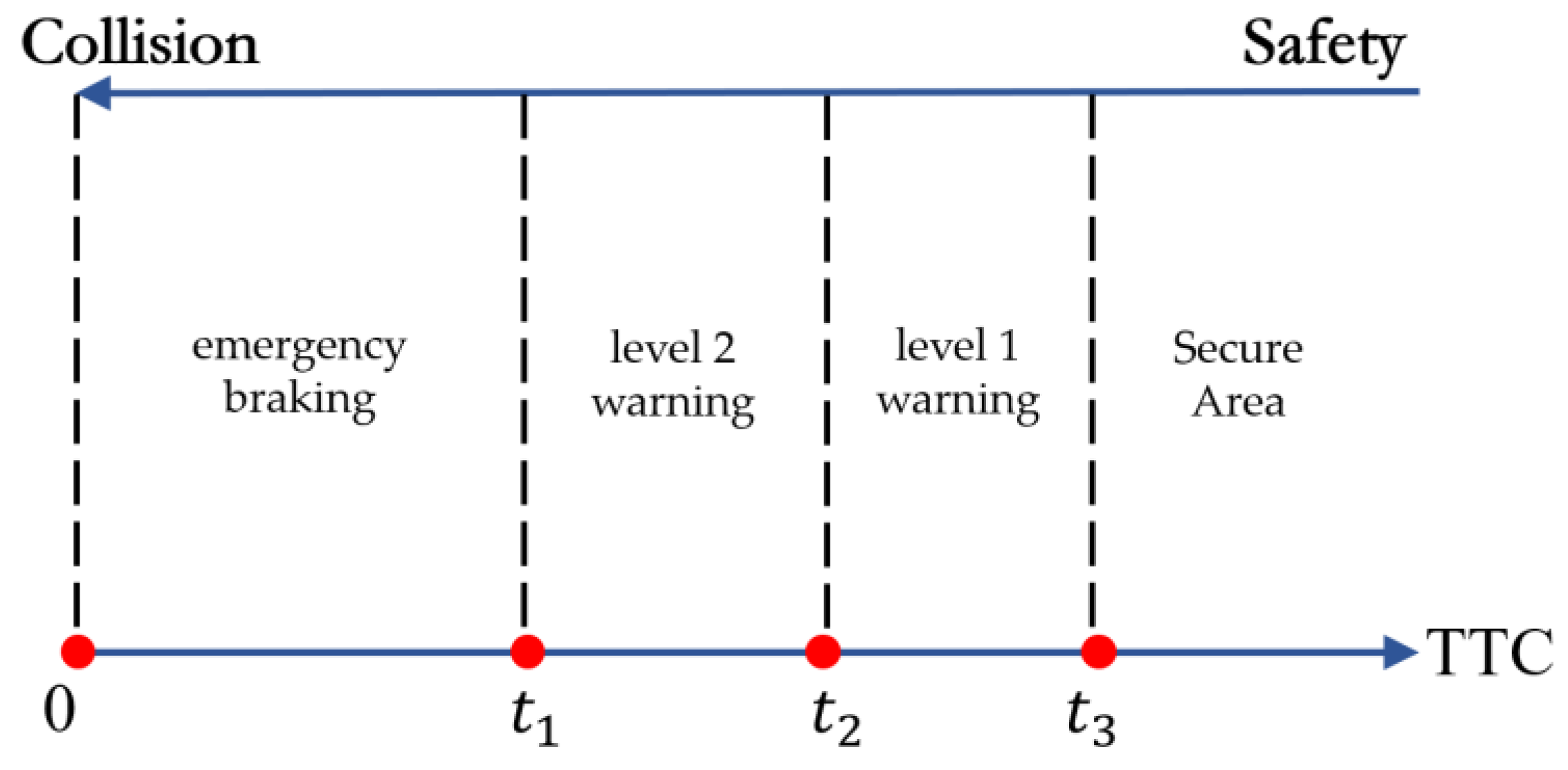
In this paper, the safety level of the vehicle is divided into “secure area (SA)”,” level 1 warning (L1)”, “level 2 warning (L2)”, and “emergency braking (EB)” in terms of time and space, as shown as Figure 12. SA means that the AEBS system does not need to perform any action, L1 means that the AEBS emits an audible sound or flashes an indicator light to alert the driver of a possible safety risk, L2 means that the driver does not perform a braking operation, and the AEBS brakes with a small deceleration to alert the driver, while eliminating the gap in the braking system and preparing for the possible emergency braking that follows. EB means that the vehicle brakes with the maximum deceleration that the AEBS can achieve to ensure the safety of the vehicle.

2.3.1. TTC Calculation and Braking Deceleration Decision

A combination of the safety time model and safety distance model is used for the control of braking intervention. First, the safety distance model is used to determine the L2 warning distance from the vehicle, and then the time to collision (TTC) equation, which considers the relative acceleration, is used to calculate the current TTC value as the threshold value for the AEBS to trigger the secondary warning; this is used to determine the time point for the braking intervention. The relative motion process of the two vehicles is simplified, i.e., the host vehicle and target vehicle are in linear motion maintaining the current velocity and acceleration until the two vehicles collide.

$$TTC=\{\begin{array}{cc}\frac{D_{rel}}{v_{rel}}& (v_{rel}>0,a_{rel}=0)\\ \frac{-v_{rel}+\sqrt{v_{rel}{}^2+2a_{rel}{D}_{rel}}}{a_{rel}}& \left(v_{rel}\ge 0,a_{rel}\ne 0\right)\\ & \mathrm{or}(v_{rel}<0,a_{rel}>0)\\ c& else\end{array}$$

(25)

where $v_{rel}=v_{HV}-v_{TV}$ is the relative velocity, $a_{rel}=a_{HV}-a_{TV}$ is the relative acceleration, $D_{rel}$ is the relative distance, $v_{rel}^2+2\cdot a_{rel}\cdot D_{rel}\ge 0$, and $c$ is a constant and is greater than the set TTC threshold value.

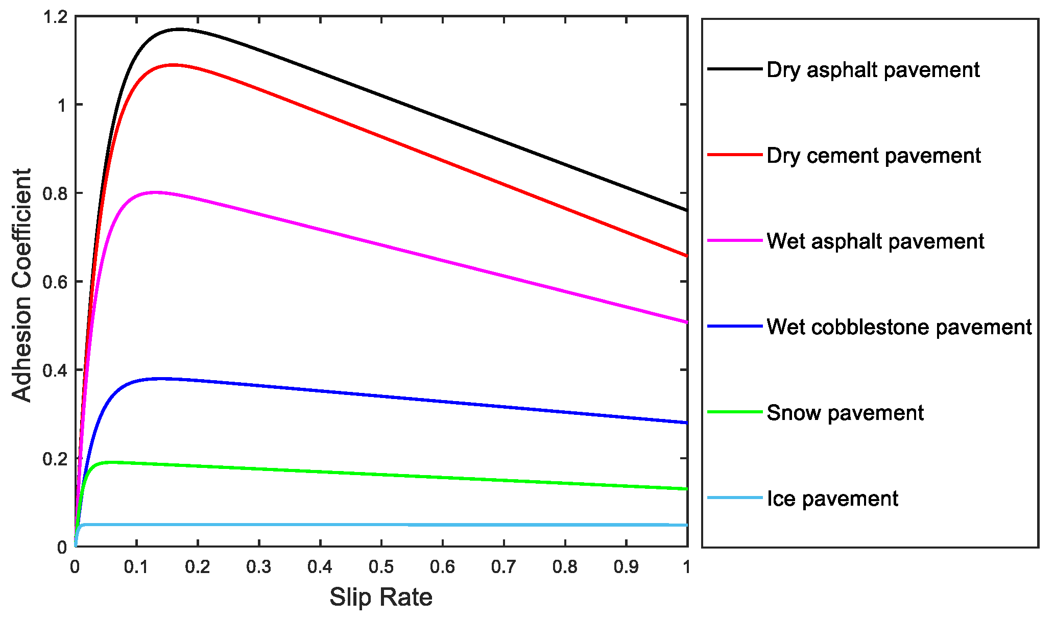
In the AEBS emergency braking stage, using the tire-road friction coefficient and the influence of road grade, the ground can provide the maximum braking deceleration as follows:

$$a_{b\max }=\mu \cdot g\cdot \cos \beta +g\cdot \sin \beta$$

(26)

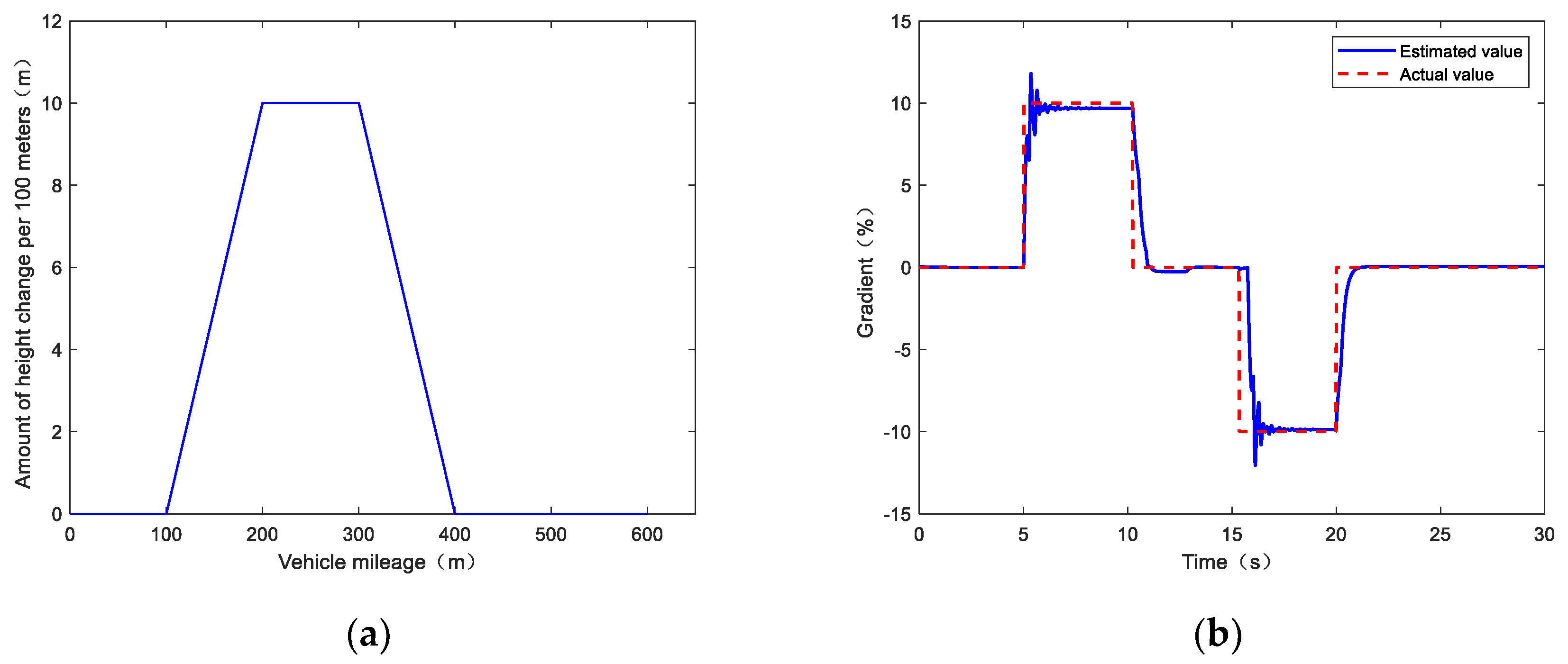
where $g$ is the gravitational constant, $\mu$ is the tire-road friction coefficient, and $\beta$ is the road grade.

In addition, NHTSA collected data on the driver’s braking deceleration during braking [26]. From the statistics, it is clear that the average value of driver braking with a deceleration of $0.55 \mathrm{g}$($5.5 \mathrm{m}/{\mathrm{s}}^2$) cumulatively was 95%.

To take into account the braking habits of the driver, the driving experience, and the collision avoidance effect of the AEBS, the braking deceleration during emergency braking of the AEBS is determined as follows (unit: $\mathrm{m}/{\mathrm{s}}^2$):

$$a_b=\min (a_{b\max },-5.5)$$

(27)

On low friction coefficient roads, the braking deceleration cannot reach $5.5 \mathrm{m}/{\mathrm{s}}^2$, and the braking deceleration at this time is determined as the maximum value that the ground can provide. On high friction roads, the braking deceleration is determined as $5.5 \mathrm{m}/{\mathrm{s}}^2$. Since there is a gap in the actuator of the commercial vehicle pneumatic braking system, which will cause a delay in the deceleration response, a certain brake deceleration is applied to the vehicle in the L2 stage to make the vehicle eliminate the braking gap and thus improve the pressure response speed in the emergency braking stage. Here, the braking deceleration of the AEBS in the secondary warning stage is determined as $1 \mathrm{m}/{\mathrm{s}}^2$.

The braking deceleration and vehicle status for each stage determined in this paper are shown in

Table 6. Braking deceleration and vehicle status in each phase.

	EB	L2	L1	SA
Braking deceleration ($\mathrm{m}/{\mathrm{s}}^2$)	$a_b$	−1	0	0
AEBS response status	Braking	Light + sound warning	Light warning	Normal driving

.

2.3.2. Braking Intervention Decision

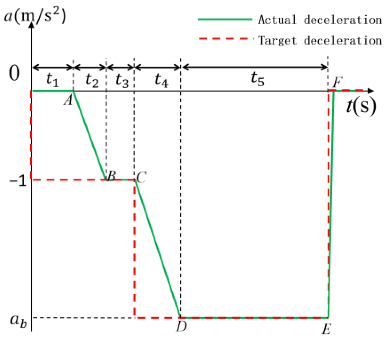
According to Table 6, we can divide the decelerated speed–time course curve of the vehicle during an AEBS system operation into six stages, as shown in Figure 13, in which the red dashed line is the current target decelerated speed of the vehicle and the green solid line is the actual decelerated speed of the vehicle. The six stages are OA (brake coordination), AB (deceleration growth), BC (continuous braking), CD (decelerated growth), DE (continuous braking), and EF (brake release). The target deceleration, vehicle speed, braking distance, and time required for each phase are shown in

Table 7. List of parameters for each braking phase.

Braking Phase	Target Deceleration $({\mathbf{m}/\mathbf{s}}^2)$	Time	Vehicle Speed	Braking Distance
OA	−1	0.2	$v_{SV,A}=v_{SV}$	$D_1=v_{SV}\cdot t_1$
AB	−1	0.2	$v_{SV,B}=v_{SV,A}+\frac{1}{2}{a}_0\cdot t_2$	$D_2=v_{SV,A}\cdot t_2+\frac{1}{6}{a}_0\cdot t_2^2$
BC	−1	0.4	$v_{SV,C}=v_{SV,B}+a_0\cdot t_3$	$D_3=\frac{{(v_{SV,C})}^2-{(v_{SV,B})}^2}{2a_0}$
CD	$a_b$	0.3	$v_{SV,D}=v_{SV,C}+\frac{1}{2}(a_b-a_0)\cdot t_4$	$D_4=v_{SV,C}\cdot t_4+\frac{1}{6}(a_b-a_0)\cdot t_4^2$
DE	$a_b$	$\frac{v_{SV,E}-v_{SV,D}}{2(a_b-a_0)}$	$v_{SV,E}=v_{TV}(t)$	$D_5=\frac{{(v_{SV,E})}^2-{(v_{SV,D})}^2}{2(a_b-a_0)}$
EF	0	0	0	$D_6=0$

.

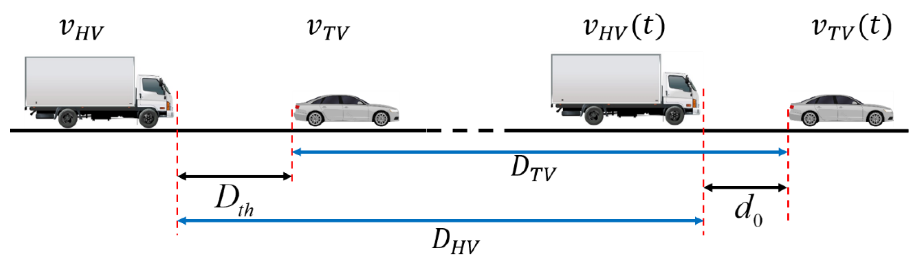
The distance between the host vehicle and the target vehicle in front of the AEBS during braking is shown in Figure 14. When $v_{HV}(t)=v_{TV}(t)$ and the relative distance is greater than $d_0$, the host vehicle enters a safe state and the AEBS releases the brake.

The L2 distance $D_{th}$ is defined as follows: when the relative distance between the two vehicles is $D_{th}$, the AEBS enters the L2 stage and brakes according to the braking process described above. When the speed of the two vehicles is the same, the distance between the host vehicle and the target vehicle is $d_0$, and $D_{th}$ is the critical L2 distance. Its calculation equation is as follows:

$$D_{th}=D_{HV}-D_{TV}+d_0$$

(28)

where $d_0$ is the reserved safety distance, $D_{HV}$ is host vehicle braking distance, and $D_{TV}$ is the driving distance of the target vehicle during the host vehicle braking process.

The reserved safety distance should be selected moderately. If $d_0$ is too large, it will hinder the efficiency of passage; if it is too small, it will affect collision avoidance. After comprehensive consideration of braking safety and efficiency factors, the reserved safety distance $d_0$ was determined to be 5 m.

Since the CCRb2 condition cannot predict the speed of the target vehicle $v_{TV}(t)$ after braking, in order to improve the safety of the AEBS, the speed when the brakes are released from the vehicle in the CCRb2 condition is set to 0. The speed when the brakes are released from the AEBS in the rest of the conditions is the same as that of the target vehicle.

$$v_{HV}(t)=\{\begin{array}{ll}0& \mathrm{CCRs}/\mathrm{CCRb}\\ v_{TV}(t)& \mathrm{CCRm} \end{array}$$

(29)

From the above analysis, the critical L2 distance $D_{th}$ is determined under different working conditions.

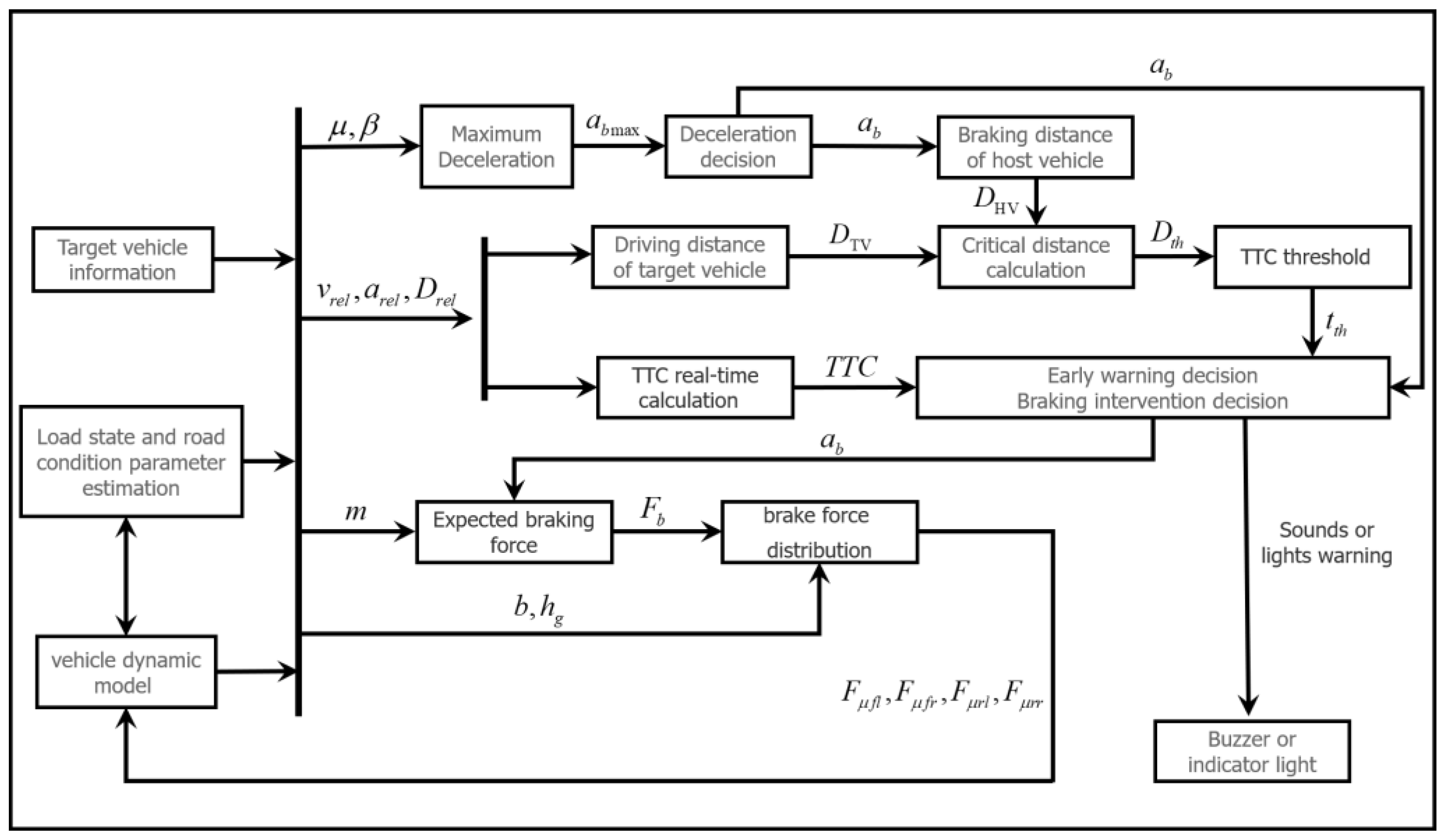
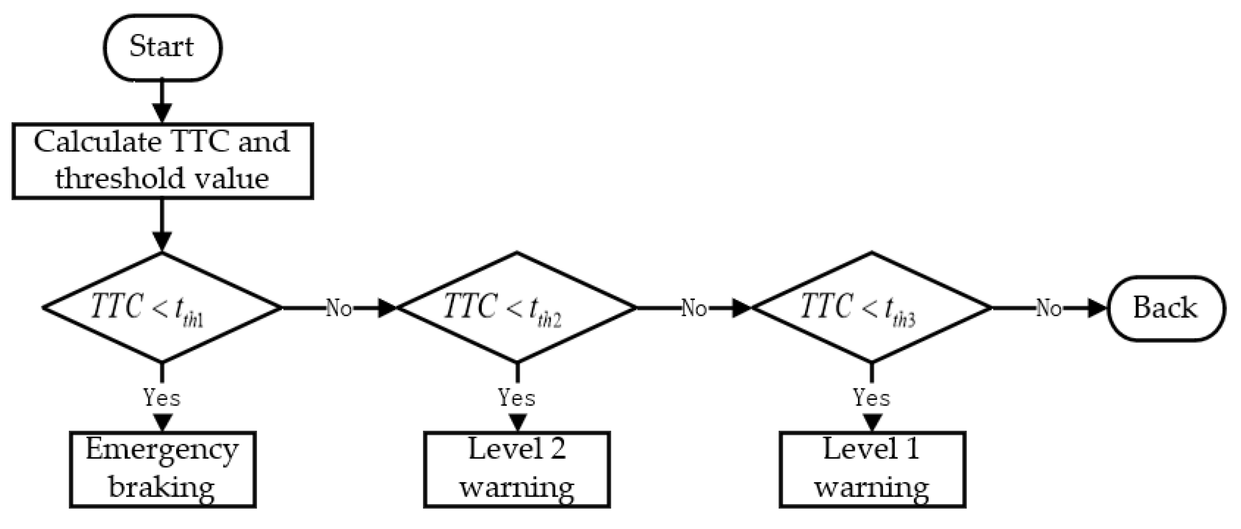
The TTC-based AEBS warning and emergency braking control flow used in this paper are shown in Figure 15.

Therefore, the task of the braking intervention timing decision is to determine the TTC threshold values for the primary warning stage, the L2 distance stage, and the emergency braking stage.

From the above analysis of the braking distance between the host vehicle and the target vehicle, it is clear that the AEBS enters the L2 stage and brakes when the relative distance between the two vehicles is $D_{th}$, and the two vehicles are finally separated by $d_0$. Therefore, $D_{th}$ is substituted into the TTC calculation equation, and the TTC value at this time is the threshold value for the L2 stage of the AEBS.

The TTC threshold value for the L2 stage determined by $D_{th}$ is as follows:

$$TT{C}_{th,\mathrm{II}}=\{\begin{array}{cc}\frac{D_{th}}{v_{rel}}& (v_{rel}>0,a_{rel}=0)\\ \frac{-v_{rel}+\sqrt{{\left(v_{rel}\right)}^2+2\cdot a_{rel}\cdot D_{th}}}{a_{rel}}& \left(\begin{array}{l}{v}_{rel}\ge 0,a_{rel}\ne 0\\ v_{rel}<0,a_{rel}>0\end{array}\right)\end{array}$$

(30)

In addition, taking into account braking safety and the driving experience, the warning time and emergency braking time of the AEBS are specified as follows:

When the TTC is greater than 4.4 s, the AEBS should not issue a collision warning. The emergency braking phase should not start before the TTC is greater than 3 s. L2 is 0.8 s before the start of emergency braking, with two modes of acoustic, optical, and tactile warning. L1 is 1.4 s before the start of emergency braking, with one mode of acoustic, optical, and tactile warning. The threshold value of the second level of warning should be less than 3.8 s.

The threshold value of the second level of warning should be less than 3.8 s.

In summary, on the basis of the warning time defined by the driving experience and the TTC threshold values for the L2 stage calculated using Equation (30), the TTC threshold values for the primary warning stage, the L2 stage, and the emergency braking stage are determined as shown in

Table 8. TTC threshold.

$\mathbf{Emergency} \mathbf{Braking} \left({\mathit{t}}_{\mathit{t}\mathit{h}1}\right)$	$\mathbf{L}2\left({\mathit{t}}_{\mathit{t}\mathit{h}2}\right)$	$\mathbf{L}1\left({\mathit{t}}_{\mathit{t}\mathit{h}3}\right)$
$\min (TT{C}_{th,\mathrm{II}},3.8)-0.8$	$\min (TT{C}_{th,\mathrm{II}},3.8)$	$\min (TT{C}_{th,\mathrm{II}},3.8)+0.6$

.

In summary, this paper uses $D_{th}$ to invert the TTC threshold value of the L2 stage of the vehicle AEBS and finally determines the TTC threshold value of each stage, so as to improve its working condition adaptability and the driver’s trust in the AEBS.

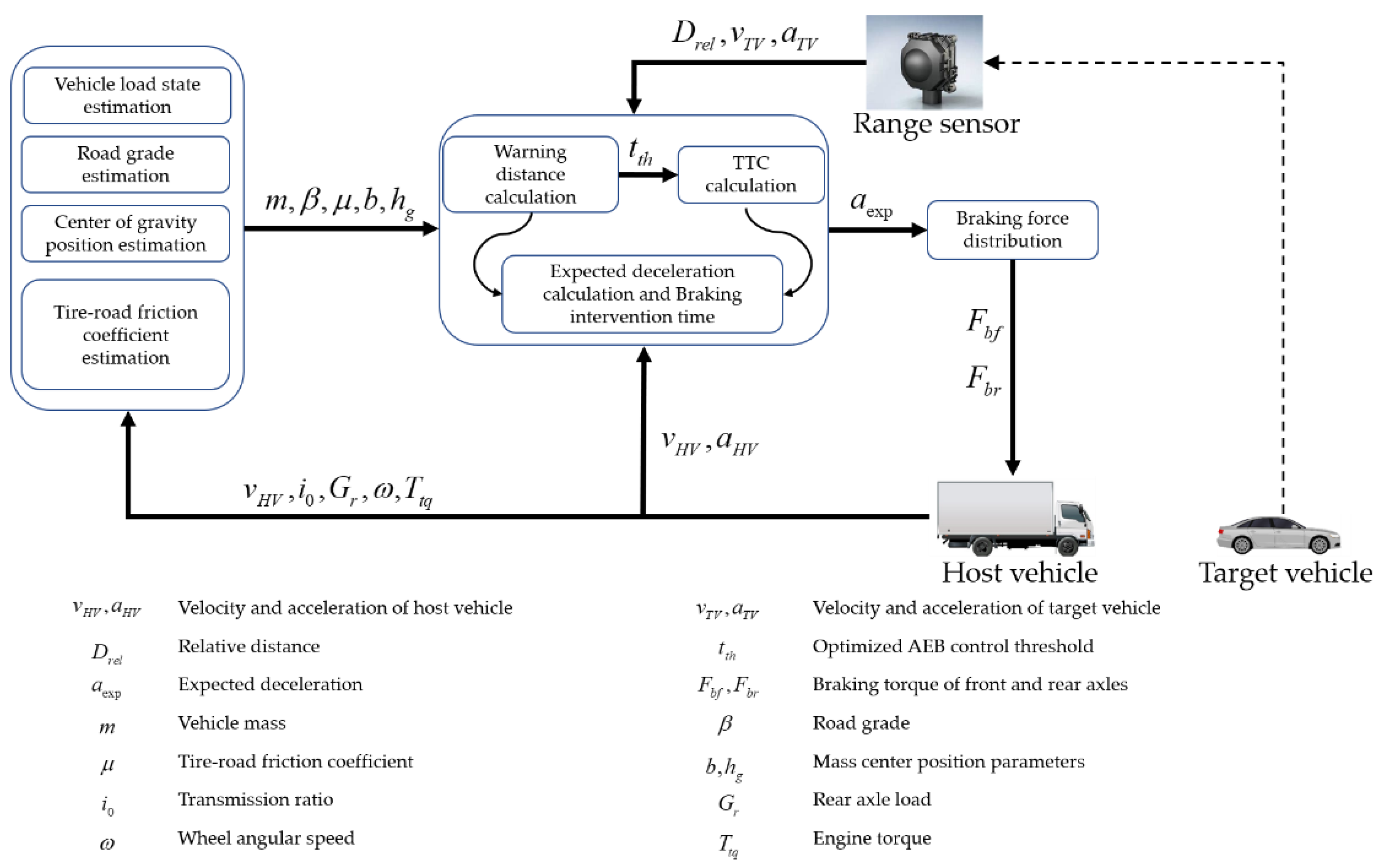
2.3.3. Braking Force Distribution Strategy

The braking force distribution between the front and rear axles affects the braking safety of the vehicle. During braking, if the rear wheels are held first, the rear axle may slip sideways, and if the front wheels are held first, the vehicle will lose steering ability. Therefore, the braking force distribution strategy should be reasonably designed to ensure that the front and rear wheels are held at the same time while making full use of tire–road friction to improve the braking stability and safety of the vehicle [29].

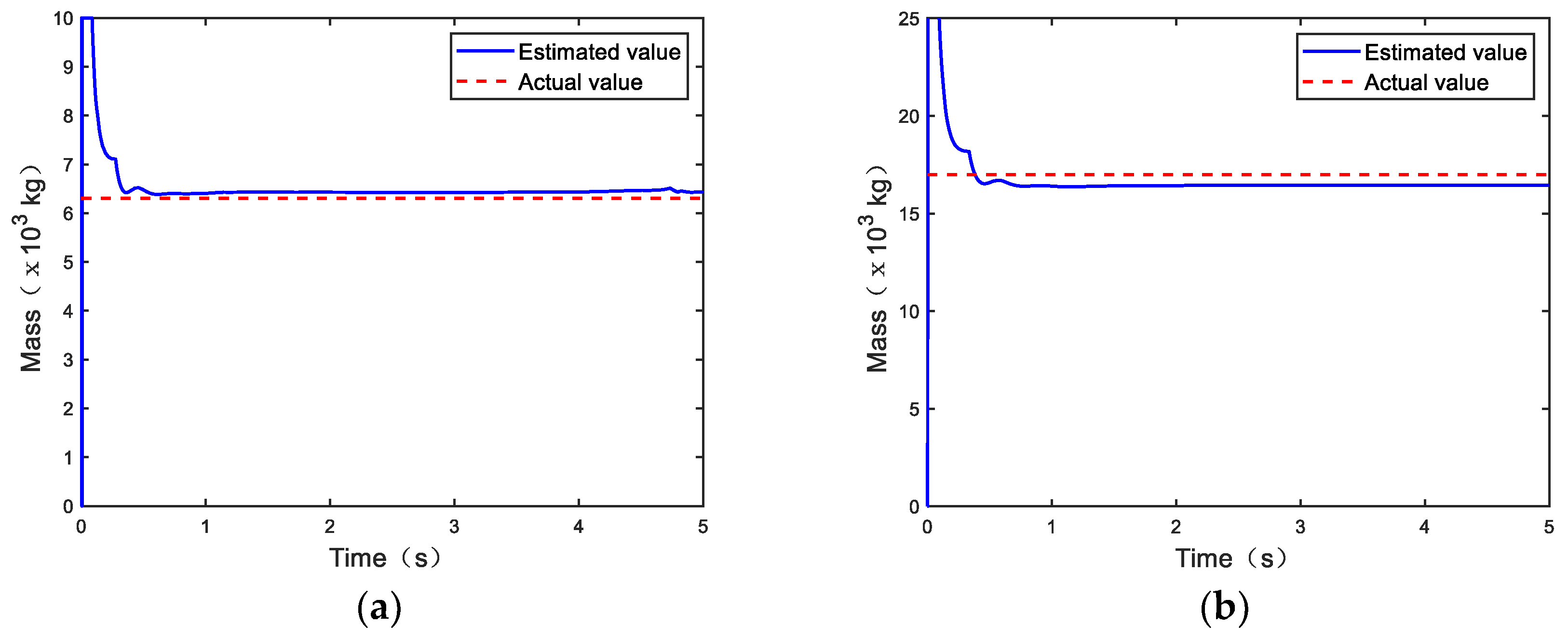
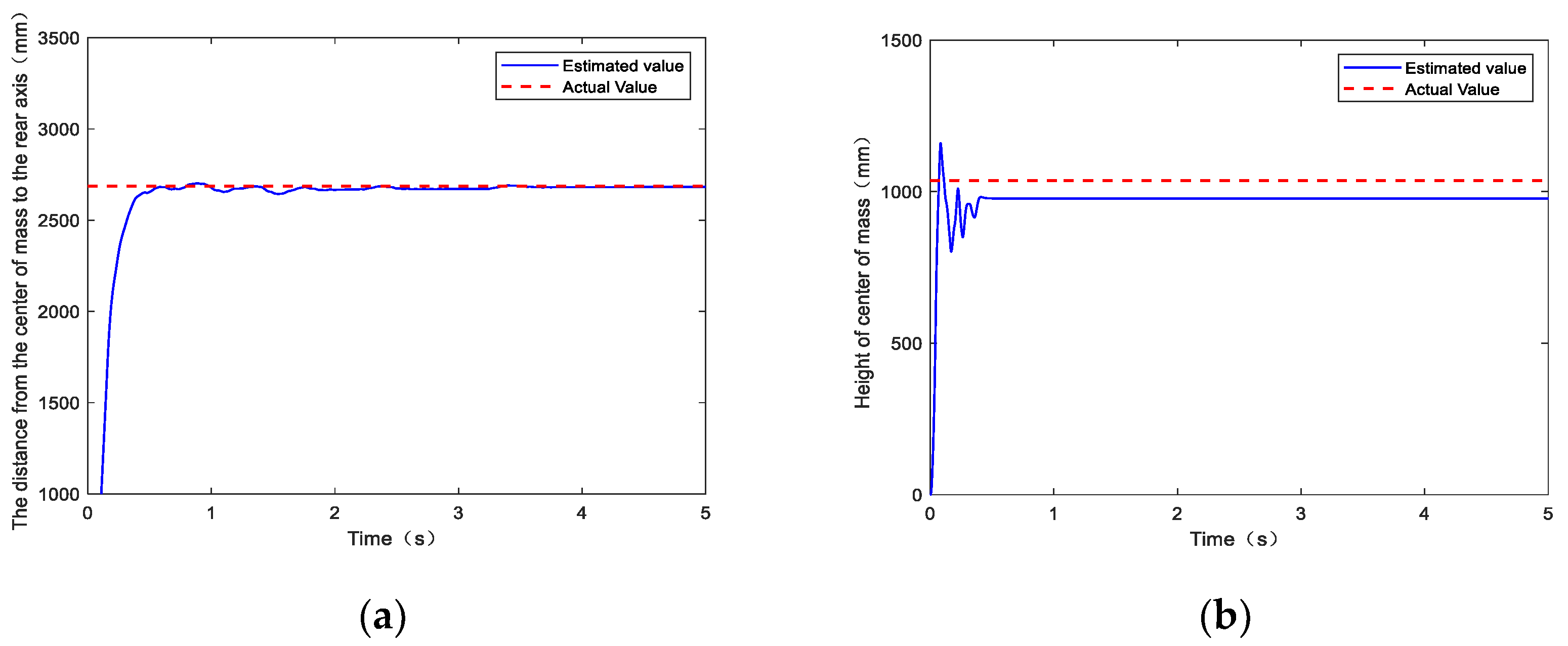
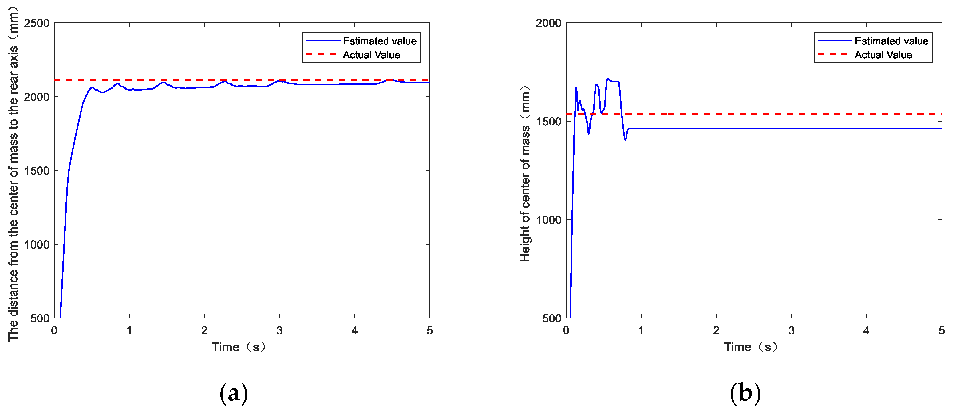
The braking force distribution strategy is based on the desired deceleration, vehicle mass, road grade, the center of gravity position, and other parameters. Firstly, the braking force required by the vehicle is determined based on the desired deceleration $a_{\exp }(a_{\exp }<0)$, the vehicle mass, and road grade of the AEBS, and then the axle load of the front and rear axles during braking is calculated and the front and rear axle braking force is distributed.

First, the braking force required by the vehicle is calculated according to Equation (31).

$$F_b=m{a}_{\exp }$$

(31)

where $m$ is the vehicle mass and $a_{\exp }$ is the desired deceleration.

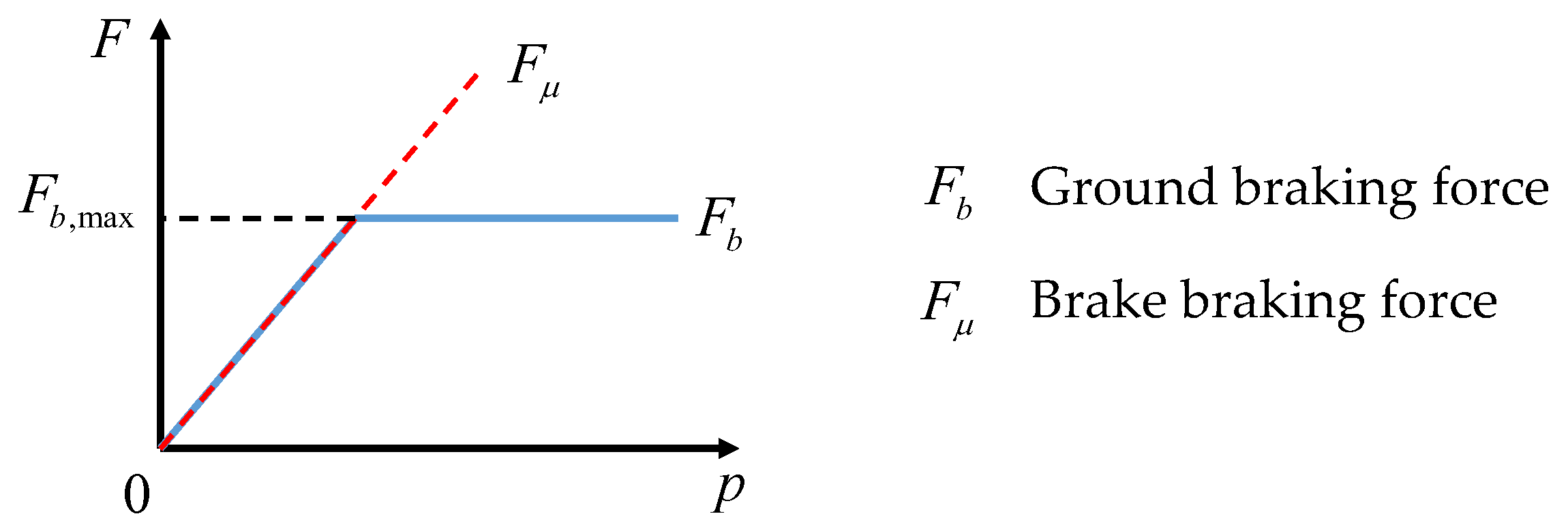
From Figure 16, when the wheel does not reach the road friction limit, the brake braking force is equal to the ground braking force, i.e., $F_{\mu }=F_b$. The total brake braking force can be determined from the total demand ground braking force.

Next, the normal force of the ground on the wheel is calculated. From the vehicle longitudinal dynamics equation, ignoring the effect of air resistance and rolling resistance, the normal reaction force of the ground on the wheels is:

$$\{\begin{array}{l}{F}_{zf}=\frac{mgb\cos \beta -(mg\sin \beta +m{a}_{\exp })h_g}{L}\\ F_{zr}=\frac{mga\cos \beta +(mg\sin \beta +m{a}_{\exp })h_g}{L}\end{array}$$

(32)

where $F_{zf}$ and $F_{zr}$ are the normal reaction forces of the ground on the front and rear wheels, respectively.

The front and rear axle braking forces are distributed according to the normal force of the ground on the wheels. When the front and rear axle braking force is distributed, it is necessary to ensure that the front and rear wheels utilize the same road friction.

$$\{\begin{array}{l}{F}_{\mu f}+F_{\mu r}=F_{\mu }\\ \frac{F_{\mu f}}{F_{zf}}=\frac{F_{\mu r}}{F_{zr}}\end{array}$$

(33)

where $F_{uf}$ and $F_{\mu r}$ are the front and rear axle braking forces at the current brake deceleration.

Finally, in regards to distributing the wheel braking force, the braking force is equally distributed between the left and right wheels of the same axle, and when braking on special roads, such as opposing roads, the braking force is adjusted by the ABS to ensure the braking safety of the vehicle as a priority.

$$\{\begin{array}{l}{F}_{\mu fr}=F_{\mu fl}=\frac{1}{2}{F}_{\mu f}\\ F_{\mu rr}=F_{\mu rl}=\frac{1}{2}{F}_{\mu r}\end{array}$$

(34)

where $F_{\mu fl}$,$F_{\mu fr}$,$F_{\mu rl}$,$F_{\mu rr}$,denote the braking force of the four wheels.

3. Construction of Test Platform

In order to verify the effectiveness and robustness of the proposed AEBS control strategy, a test platform was built.

3.1. Configuration of the Test Platform

The proposed algorithm was embedded in an RCP unit based on Simulink Real-Time, and the configuration of the test platform is shown in Figure 17. The platform is divided into four parts: the host PC, the target PC, the I/O hardware, and the brake system hardware. The initial motion states of the host vehicle and the target vehicle, and the virtual radar signals were set in TruckSim. The AEBS control strategy and the vehicle dynamics model were compiled in the host PC and sent to the target PC via the Ethernet, and the target PC was used as the carrier for the I/O hardware to complete the signal acquisition and output to the host PC. The experimental data were assessed in Matlab installed on the host PC.

The overall structure and components of the test platform are shown in Figure 18.

3.2. Test Conditions

The AEBS test was conducted under different load states, road grades, and tire-road friction coefficients. The host vehicle approached the target vehicle with different initial speeds and relative distances, and the specific test scenarios were set as shown in

Table 9. HIL test conditions.

Conditions	Load State	Friction	Grade
CCRs	No load	0.4	0
	No load	0.8	0
	Full loaded	0.4	0
	Full loaded	0.8	0
	No load	0.4	−10
	No load	0.4	0
	No load	0.4	10
CCRm	No load	0.4	0
	No load	0.8	0
	Full loaded	0.4	0
	Full loaded	0.8	0
CCRb	No load	0.8	0
	Full loaded	0.8	0

.

4. Results and Analysis

4.1. CCRs Scenario

The initial speed of the host vehicle was 40 km/h, the speed of the target vehicle was 0 km/h, and the initial distance was 120 m. The test results are shown in Figure 19.

4.2. CCRm Scenario

The initial speed of the host vehicle was 80 km/h, the speed of the target vehicle was 12 km/h, the initial distance was 120 m, and the road grade was 0%. The test results are shown in Figure 20.

4.3. CCRb Scenario

The road grade was 0%, $\mu =0.8$, the initial distance was 40 m, the speed of the host vehicle was 50 km/h, the speed of the target vehicle was 50 km/h, and the target vehicle applied a $4 \mathrm{m}/{\mathrm{s}}^2$ deceleration at t = 4 s. The test results are shown in Figure 21.

The performance of the proposed AEBS was evaluated for various load states, road grades, and friction conditions, and the results are listed in the right part of Figure 19, Figure 20 and Figure 21. The performance of the fixed threshold strategy is shown in the left part and is compared with the proposed system.

The desired distance after AEBS activation was set to 5 m from the target. In the CCRs scenario, the two control strategies were able to ensure that the vehicle did not collide, but under the condition of $\mu =0.8$, the distance between the two vehicles when parking for the fixed threshold strategy was close to 20 m. The proposed AEBS maintained a parking distance of approximately 5 m regardless of the attachment conditions, which improved the utilization rate and traffic efficiency of the road space. In the CCRm test, the fixed threshold strategy was not able to avoid the occurrence of collisions, as shown in Figure 20(9). The method proposed in this paper had entered into the early warning state by 0.2 s, and braked with a maximum deceleration 0.5 s in advance to avoid a collision. In the CCRb scenario, the control strategy proposed in this paper maintained the maximum deceleration at $5.5m/s^2$, which would ensure a comfortable driving experience for the driver and passengers.

5. Conclusions

In this study, an analysis of the vehicle driving condition was added to the control strategy, in which the relevant parameters are estimated and simulated. In our method, the least-squares estimation method of vehicle mass based on the starting condition was used to estimate the actual mass of the vehicle, and the current road grade was estimated in real time based on the mass estimation result. The CKF method was used to estimate the center of gravity position and the estimation result was applied to the braking force distribution. The $\mu -\lambda$ model combined with the gradient of the $\mu -\lambda$ curve was used to estimate the road friction coefficient, and the estimation accuracy of the above parameters was guaranteed in real time. The $\mu -\lambda$ model and the gradient of the $\mu -\lambda$ curve were combined to estimate the tire-road friction coefficient. The AEBS control strategy improved the adaptability to the working conditions and decision-making rationality.

After the AEBS control strategy completed the decision and output the deceleration demand, the front and rear axle braking force was distributed by combining the current actual load and the center of gravity position of the vehicle. This ensures the braking stability of the vehicles, while making full use of the road friction conditions, and improves the control robustness of the AEBS.

The experimental results show that the proposed AEBS control strategy can guarantee a good control effect under different load conditions and road conditions. The AEBS proposed in this paper did not collide in any test scenario. The proposed AEBS maintains a parking distance of approximately 5 m regardless of the attachment conditions. When the fixed threshold strategy cannot avoid collision, the AEBS proposed in this paper enters the early warning state within 0.2 s, and brakes with maximum deceleration 0.5 s in advance to avoid a collision. The control strategy proposed in this paper maintains the maximum deceleration of $5.5 \mathrm{m}/{\mathrm{s}}^2$, which would ensure a comfortable driving experience for the driver and passengers.

References

1. Qiu, C.; Wang, G.; Meng, M.; Shen, Y. A Novel Control Strategy of Regenerative Braking System for Electric Vehicles under Safety Critical Driving Situations. Energy 2018, 149, 329–340. [Google Scholar] [CrossRef]
2. Graba, M.; Mamala, J.; Bieniek, A.; Sroka, Z. Impact of the Acceleration Intensity of a Passenger Car in a Road Test on Energy Consumption. Energy 2021, 226, 120429. [Google Scholar] [CrossRef]
3. Cicchino, J.B. Effectiveness of Forward Collision Warning and Autonomous Emergency Braking Systems in Reducing Front-to-Rear Crash Rates. Accid. Anal. Prev. 2017, 99, 142–152. [Google Scholar] [CrossRef] [PubMed]
4. Petin, V.V.; Keller, A.V. Modeling the Algorithm of the Automatic Emergency Braking System with the Prediction of the Coefficient of Tire Grip. IOP Conf. Ser. Mater. Sci. Eng. 2020, 819, 012012. [Google Scholar] [CrossRef]
5. Momiyama, F.; Kitazawa, K.; Miyazaki, K.; Soma, H.; Takahashi, T. Gravity Center Height Estimation for the Rollover Compensation System of Commercial Vehicles. JSAE Rev. 1999, 20, 493–497. [Google Scholar] [CrossRef]
6. Han, I.C.; Luan, B.C.; Hsieh, F.C. Development of Autonomous Emergency Braking Control System Based on Road Friction; Hua-Chung Automobile Information Technical Center Co., Ltd.: New Taipei City, Taiwan, 2014. [Google Scholar]
7. Park, M.-K.; Lee, S.-Y.; Kwon, C.-K.; Kim, S.-W. Design of Pedestrian Target Selection with Funnel Map for Pedestrian Aeb System. IEEE Trans. Veh. Technol. 2017, 66, 3597–3609. [Google Scholar] [CrossRef]
8. Kidambi, N.; Pietron, G.M.; Boesch, M.; Fujii, Y.; Wang, K.W. Accuracy and Robustness of Parallel Vehicle Mass and Road Grade Estimation. SAE Int. J. Veh. Dyn. Stab. NVH 2017, 1, 317–325. [Google Scholar] [CrossRef]
9. Mahyuddin, M.N.; Na, J.; Herrmann, G.; Ren, X.; Barber, P. Adaptive Observer-Based Parameter Estimation with Application to Road Gradient and Vehicle Mass Estimation. IEEE Trans. Ind. Electron. 2014, 61, 2851–2863. [Google Scholar] [CrossRef] [Green Version]
10. McIntyre, M.L.; Ghotikar, T.J.; Vahidi, A.; Song, X.; Dawson, D.M. A Two-Stage Lyapunov-Based Estimator for Estimation of Vehicle Mass and Road Grade. IEEE Trans. Veh. Technol. 2009, 58, 3177–3185. [Google Scholar] [CrossRef]
11. Mun, H.; Kim, B. A Study on the V2v-Communication-Based Aeb System for High-Speed Driving under Various Road Surface Conditions. In Advanced Multimedia and Ubiquitous Engineering; Springer: Berlin/Heidelberg, Germany, 2016; Volume 2, pp. 247–252. [Google Scholar]
12. Sevil, A.O.; Canevi, M.; Soylemez, M.T. Development of an Adaptive Autonomous Emergency Braking System Based on Road Friction; Istanbul Technical University: Istanbul, Turkey, 2019. [Google Scholar]
13. Pohl, A.; Steindl, R.; Reindl, L. Intelligent Tire’ Utilizing Passive Saw Sensors—Measurement of Tire Friction. IEEE Trans. Instrum. Meas. 1999, 48, 1041–1046. [Google Scholar] [CrossRef]
14. Tuononen, A. On-Board Estimation of Dynamic Tyre Forces from Optically Measured Tyre Carcass Deflections. Int. J. Heavy Veh. Syst. 2009, 16, 362–378. [Google Scholar] [CrossRef] [Green Version]
15. Bian, M.; Chen, L.; Luo, Y.; Li, K. A Dynamic Model for Tire/Road Friction Estimation under Combined Longitudinal/Lateral Slip Situation; Tsinghua University: Beijing, China, 2014. [Google Scholar]
16. Choi, M.; Oh, J.J.; Choi, S.B. Linearized Recursive Least Squares Methods for Real-Time Identification of Tire-Road Friction Coefficient. IEEE Trans. Veh. Technol. 2013, 62, 2906–2918. [Google Scholar] [CrossRef]
17. Xin, W.; Liang, G.; Mingming, D.; Xiaolei, L. State Estimation of Tire-Road Friction and Suspension System Coupling Dynamic in Braking Process and Change Detection of Road Adhesive Ability. Proc. Inst. Mech. Eng. Part D J. Automob. Eng. 2022, 236, 1170–1187. [Google Scholar] [CrossRef]
18. Yang, W.; Zhang, X.; Lei, Q.; Cheng, X. Research on Longitudinal Active Collision Avoidance of Autonomous Emergency Braking Pedestrian System (Aeb-P). Sensors 2019, 19, 4671. [Google Scholar] [CrossRef] [PubMed] [Green Version]
19. Cicchino, J.B.; Zuby, D.S. Characteristics of Rear-End Crashes Involving Passenger Vehicles with Automatic Emergency Braking. Traffic Injury Prevention 2019, 20, S112–S118. [Google Scholar] [CrossRef] [PubMed] [Green Version]
20. Chen, Y.L.; Shen, K.Y.; Wang, S.C. Forward Collision Warning System Considering Both Time–to–Collision and Safety Braking Distance. Int. J. Veh. Saf. 2013, 6, 347–360. [Google Scholar] [CrossRef]
21. Abdullah, Z.; Heerwan, P.M.; Izhar, I.M.; Zakaria, M.A. Study the Influence of Distance in Artificial Potential Field (Apf) for Autonomous Emergency Braking System (Aeb) on Longitudinal Motion. IOP Conf. Ser. Mater. Sci. Eng. 2021, 1068, 012015. [Google Scholar] [CrossRef]
22. Kim, H.; Shin, K.; Chang, I.; Huh, K. Autonomous Emergency Braking Considering Road Slope and Friction Coefficient. Int. J. Automot. Technol. 2018, 19, 1013–1022. [Google Scholar] [CrossRef]
23. Guo, J.; Zhang, H. Collision Avoidance Strategy of High-Speed Aeb System Based on Minimum Safety Distance; SAE Technical Paper Series; SAE: Warrendale, PA, USA, 2021. [Google Scholar]
24. Zhou, W.; Wang, X. Calibrating and Comparing Autonomous Braking Systems in Motorized-to-Non-Motorized-Vehicle Conflict Scenarios. IEEE Trans. Intell. Transp. Syst. 2022, 1–16. [Google Scholar] [CrossRef]
25. McGehee, D.V.; Brown, T.L.; Lee, J.D.; Wilson, T.B. Effect of Warning Timing on Collision Avoidance Behavior in a Stationary Lead Vehicle Scenario. Transp. Res. Rec. 2002, 1803, 1–6. [Google Scholar] [CrossRef]
26. McLaughlin, S.B. Analytic Assessment of Collision Avoidance Systems and Driver Dynamic Performance in Rear-End Crashes and Near-Crashes; Virginia Polytechnic Institute and State University: Blacksburg, VA, USA, 2007. [Google Scholar]
27. He, Y.; Lu, C.; Shen, J.; Yuan, C. Design and Analysis of Output Feedback Constraint Control for Antilock Braking System Based on Burckhardt’s Model. Assem. Autom. 2019, 39, 497–513. [Google Scholar]
28. Zhao, J.; Zhang, J.; Zhu, B. Development and Verification of the Tire/Road Friction Estimation Algorithm for Antilock Braking System. Math. Probl. Eng. 2014, 2014, 786492. [Google Scholar] [CrossRef] [Green Version]
29. Jin, X.; Wang, J.; Yan, Z.; Xu, L.; Yin, G.; Chen, N. Robust Vibration Control for Active Suspension System of in-Wheel-Motor-Driven Electric Vehicle Via Μ-Synthesis Methodology. J. Dyn. Syst. Meas. Control 2022, 144, 051007. [Google Scholar] [CrossRef]
Figure 1. Control framework of the AEBS.
Machines 10 00895 g001
Figure 2. AEBS simulation platform architecture.
Machines 10 00895 g002
Figure 3. Vehicle load state and road grade estimation schematic.
Machines 10 00895 g003
Figure 4. Flowchart of vehicle start state discrimination.
Machines 10 00895 g004
Figure 5. Mass estimation based on the starting state of the vehicle. (a) Unladen mass estimation results; (b) full load mass estimation results.
Machines 10 00895 g005
Figure 6. (a) Schematic diagram of road height variation with mileage; (b) road grade estimation results.
Machines 10 00895 g006
Figure 7. Estimation results of the center of gravity position of the vehicle without a load. (a) Distance from the center of gravity position to the rear axis; (b) height of the center of gravity.
Machines 10 00895 g007
Figure 8. Estimation results of the center of gravity position of the vehicle at full load. (a) Distance from the center of gravity position to the rear axis; (b) height of the center of gravity.
Machines 10 00895 g008
Figure 9. μ - λ relationship curve.
Machines 10 00895 g009
Figure 10. Tire-road friction coefficient estimation results. (a) Estimation results for μ = 0.4; (b) estimation results for μ = 0.6; (c) estimation results for μ = 0.8.
Machines 10 00895 g010
Figure 11. AEBS decision layer control strategy architecture.
Machines 10 00895 g011
Figure 12. Vehicle safety status division.
Machines 10 00895 g012
Figure 13. AEBS target deceleration and actual deceleration.
Machines 10 00895 g013
Figure 14. Vehicle distance diagram.
Machines 10 00895 g014
Figure 15. TTC-based AEBS control flow.
Machines 10 00895 g015
Figure 16. Relationship between ground braking force and brake braking force.
Machines 10 00895 g016
Figure 17. Configuration of the test platform.
Machines 10 00895 g017
Figure 18. Physical display of the test platform.
Machines 10 00895 g018
Figure 19. Comparison of experimental results for the CCRs scenario.
Machines 10 00895 g019aMachines 10 00895 g019b
Figure 20. Comparison of the experimental results for the CCRm scenario.
Machines 10 00895 g020
Figure 21. Comparison of experimental results for the CCRb scenario.
Machines 10 00895 g021