Article

Integrated Control for Path Tracking and Stability Based on the Model Predictive Control for Four-Wheel Independently Driven Electric Vehicles

1
Guilin University of Aerospace Technology, Guilin 541004, China
2
School of Mechanical and Electrical Engineering, Guilin University of Electronic Technology, Guilin 541004, China
*
Author to whom correspondence should be addressed.
Machines 2022, 10(10), 859; https://doi.org/10.3390/machines10100859
Submission received: 22 July 2022 / Revised: 18 September 2022 / Accepted: 21 September 2022 / Published: 26 September 2022
(This article belongs to the Special Issue Advanced Modeling, Analysis and Control for Electrified Vehicles)

Abstract

:
Four-wheel independently driven electric vehicles are prone to rollover when driving at high speeds on high-adhesion roads and to sideslip on low-adhesion roads, increasing the risks associated with such vehicles. To solve this problem, this study proposes a path tracking and stability-integrated controller based on a model predictive control algorithm. First, a vehicle planar dynamics model and a roll dynamics model are established, and the lateral velocity, yaw rate, roll angle, and roll angle velocity of the vehicle are estimated based on an unscented Kalman filter. The lateral stiffness of the tires is estimated online according to the real-time feedback state of the vehicle. Then, the path tracking controller, roll stability controller, and lateral stability controller are designed. An integrated control strategy is designed for the path tracking and stability, and the conditions and coordination strategies for the vehicle roll and lateral stability state in the path tracking are studied. The simulation results show that the proposed algorithm can effectively limit the lateral load transfer rate on high-adhesion roads and the sideslip angle on low-adhesion roads at high speeds. Hence, the driving stability of the vehicle under different road adhesion coefficients can be ensured and the path tracking performance can be improved.

1. Introduction

Compared with other driving vehicles, a four-wheel independently driven electric vehicle (FWID EV) has a simple structure with an in-wheel motor or wheel-side motor as a direct power source. This improves the energy transfer efficiency and the torque responds quickly. These advantages provide a basis for achieving a better stability control performance. Therefore, FWID EVs have become the focus of many researchers [1,2,3,4,5,6].
When a vehicle is driving on a wet road at high speed, improper driving can easily cause the lateral instability of the vehicle, making the vehicle sideslip and tail-flick and eventually lead to traffic accidents. Several scholars have studied the problems of vehicle sideslips and instability. In [7], the lateral control of a vehicle with longitudinal velocity variations was investigated. An improved proportional-integral control law was proposed and optimized to improve the lateral stability and handling performance of the vehicle. A new hybrid stability control system was proposed in [8] for avoiding vehicle skidding. The system controlled the lateral acceleration and the yaw moment of the vehicle which, according to the vehicle information compensated for the steering characteristics, thereby improving the steering performance. In [9], an H-infinity-based delay-tolerant linear quadratic regulator control strategy was proposed. The lateral movement and stability of the FWID EV as affected by time-varying delays were better solved. In [10], a switching strategy, composed of an error judgment strategy and a model matching strategy, was used to identify the working environment of the vehicle. In [11], a switched control strategy of the front wheel active steering and external yaw moment coordination was adopted to achieve vehicle stability under limited handling conditions. In [12], a stability controller for a high-rise vehicle based on the parametric MPC was proposed to improve the lateral stability.
In addition, it is easy to rollover when a vehicle turns sharply at high speed on a high-adhesion-coefficient road. Therefore, vehicle rollovers have attracted increasing attention in the context of serious traffic accidents. Many researchers have conducted extensive research in the recent years to reduce the harm caused by vehicle rollovers and improve the safe driving performance of vehicles. In [13], an improved sliding mode control strategy based on a state observer was proposed. It ensured that the lane-keeping errors and roll angle remained within a specified performance range. The contour lines of the load transfer ratio (CL-LTR) and the CL-LTR-based vehicle rollover index (CLRI) were proposed in [14]. Based on the CLRI, the rollover prediction for a vehicle is enhanced and the vehicle stability is improved. In [15], a control method for the rollover mitigation based on a rollover index/lateral stability was proposed. The method decreased the risk of rollover under the premise of ensuring the lateral stability of the vehicle. In [16], a double-layer dynamic decoupling control system (DDDCS), composed of an upper dynamic decoupling unit (DDU) and a lower steering control unit (SCU), was proposed to ensure the yaw stability of vehicles.
With increasing investigations on intelligent vehicles, vehicle path tracking control has become a research hotspot. The purpose of a path tracking control is to provide accurate tracking and stability control under the intervention of control algorithms. At present, researchers have used many control algorithms for vehicle path tracking control. In [17], a robust model predictive control (MPC) strategy based on a finite time domain was proposed to manage the parameter uncertainty and external disturbances in a vehicle model, thereby ensuring vehicle stability. A robust H∞ output feedback control strategy was designed in [18] and the uncertainties of the vehicle lateral velocity, yaw rate, and road curvature were considered for the path tracking. In [19], a multi-core reinforcement learning method was proposed and achieved better performance in terms of the path tracking accuracy and smoothness. In [20], an optimal path tracking extended model predictive control (MPC) scheme with multiple constraints and a vehicle-road dynamics synthesis model was proposed to improve the ride comfort and stability of the vehicle path tracking.
With the development of vehicle intelligence, more stringent requirements have been proposed for vehicle dynamic state estimations. It is difficult for low-cost sensors to accurately measure the values of certain state variables of vehicles in real time. However, in practical engineering problems, the state variables that cannot be measured directly are nevertheless required by the controller. To solve such problems, these difficult-to-measure state parameters can be obtained through a state estimation method, which further expands the use range of the vehicle sensors while reducing their use [21]. Thus, to solve the above problems, we must obtain the vehicle state parameters using a state estimation method. At present, the main methods available include sliding-mode estimation methods [22], least-squares estimation methods [23], and Kalman filter estimation methods. In [24], looking at the problem that certain state variables of underwater vehicles cannot be measured directly, Cui designed an adaptive multi-input multi-output extended state observer to estimate the unmeasured state variables. In [25], Ma studied the parameter estimation problem of a multi-variable output-error-like system with an autoregressive moving average noise, and proposed a least-squares-based iterative algorithm for an iterative search to solve a problem concerning unknown variables in the information vector. The Kalman filter equation is in a recursive form in the time domain, and thus there is no need to store large amounts of data when solving the equation; therefore, the Kalman filter method is widely used because of its fast operation speed and good real-time performance. In [26], an unscented Kalman filter (UKF) algorithm, based on the measurable variables was proposed. In this algorithm, the difficult-to-measure real-time state variables on the vehicle were estimated to provide accurate values for an integrated controller. A new integrated Kalman filter method was proposed in [27]; this method used only low-cost hardware, such as a GPS/inertial navigation system/wheel speed sensor to estimate the dynamic state of the vehicle. In [28], a bicycle dynamics-based extended Kalman filter was proposed to eliminate the influences of inertial sensor drifts.
It can be seen that researchers have made many achievements in the path tracking the control, the vehicle roll stability control, and the lateral stability control; however, many problems still need to be addressed. For example, when a vehicle tracks a desired path, it is necessary to combine the lateral stability control and rolling stability control to achieve the stability-integrated control in the path tracking. Simultaneously, it is necessary to consider ways to design a smooth switching integrated control strategy for the integrated controller to improve the adaptability of the integrated controller under different working conditions. With the aim to solving the above problems, the main objectives of this study are as follows.
(1) For the proposed integrated controller, a smooth switching strategy is designed for the stability controller such that the stability of the vehicle path tracking is better guaranteed under different road adhesion coefficients.
(2) For the vehicle parameter estimation, a planar four-wheel dynamic model and roll dynamic model of the vehicle are established. A vehicle state observer is then designed based on the UKF algorithm, and the lateral velocity, yaw rate, roll angle, and roll angle velocity are estimated in real time. The tire cornering stiffness is estimated online according to the state of the vehicle’s real-time feedback.
(3) The vehicle path tracking controller design is based on the vehicle planar four-wheel dynamic model. The MPC path tracking controller is established to output the desired front wheel angle to ensure that the vehicle can track the desired path under different road adhesion coefficients.
(4) In the vehicle roll stability controller design, based on the roll dynamics model of the vehicle, the MPC roll stability controller is established to realize the vertical load coefficient constraint of the vehicle and ensure the roll stability of the vehicle on a high-speed high-adhesion road.
(5) For the vehicle lateral stability controller design, based on the planar four-wheel dynamic model of the vehicle, the MPC lateral stability controller is established to enforce the constraint of the sideslip angle and ensure the lateral stability of the vehicle on a low-attachment road at high speed.
The remainder of this paper is organized as follows. Section 2 discusses the method adopted to build the vehicle planar dynamics model and the vehicle roll dynamics model. The vehicle state and the tire cornering stiffness are estimated in Section 3. The proposed integrated controller is described in Section 4. Section 5 presents the verification of the effectiveness of the proposed controller through simulations. The conclusions are presented in Section 6.

2. Vehicle Dynamics Model

2.1. Vehicle Planar Dynamics Model

To better study the stability control problem, a vehicle planar four-wheel dynamics model is established, as shown in Figure 1. Using this model, the longitudinal, lateral, and yaw moment dynamic equations are established. The specific equations are as follows:
v ˙ x - v y r = 1 m ( F x f r cos δ + F x f l cos δ F y f r sin δ F y f l sin δ + F x r l + F x r r ) ,
v ˙ y + v x r = 1 m ( F x f r sin δ + F x f l sin δ + F y f r cos δ + F y f l cos δ + F y r l + F y r r ) ,
r ˙ = 1 I z [ l f F x f l + F x f r sin δ + t f 2 F y f l F y f r sin δ l r F y r l + F y r r + l f F y f l + F y f r cos δ t f 2 F x f l F x f r cos δ t r 2 F x r l F x r r ]
In the above equations, m is the vehicle mass; r , v x , and v y are the yaw rate, longitudinal velocity, and lateral velocity of the vehicle, respectively; δ is the front wheel angle; β is the vehicle sideslip angle; I z is the rotational inertia of the vehicle around the Z-axis; l represents the distance from the vehicle center of mass ( C . G ) to the front and rear axles ( = f ( f r o n t ) , = r ( r e a r ) ); t represents the wheel track of the front and rear wheels ( = f , r ) ; and F y i j and F x i j represent the lateral and longitudinal forces of the four wheels, respectively, ( i j = f l left-front wheel), f r (right-front wheel), r l (left-rear wheel), r r (right-rear wheel).
The motion balance equation of the vehicle in the global coordinate system can be expressed as follows:
V Y = v x sin ψ + v y cos ψ V X = v x cos ψ v y sin ψ ,
where, ψ is the heading angle of the vehicle.
To reduce the calculation amounts for the control algorithm in the vehicle lateral and roll stability controller and to meet the real-time requirements, the model is simplified to a monorail dynamic model. The simplified vehicle differential equations are as follows:
v ˙ y = 1 m C α f α f cos δ + C α r α r v x r ,
r ˙ = 1 I z l f C α f α f cos δ l r C α r α r + 1 I z M F x   ,
where C α f and C α r are the lateral stiffnesses of the front and rear wheels, respectively; α f is the front wheel sideslip angle; α r is the sideslip angle of the rear wheel; and M F x is the additional yaw moment. M F x can be defined as follows:
M F x = l f R sin δ T f r + T f l + t f 2 R cos δ T f r T f l + t r 2 R T r r T r l ,
where, R represents the effective wheel radius, and T i j ( i j = f l ,   f r ,   r l ,   r r ) represents the driving torque of the four wheels.
The lateral dynamics equation for the vehicle is expressed as follows:
v ˙ y = a y r v x .
The lateral acceleration is defined as follows:
a y = 1 m C α f α f cos δ + C α r α r .
The longitudinal and lateral forces of the tire are calculated using linear expressions. These can be expressed as follows:
F x f l = F x f r = C l f λ f j ,
F x r l = F x r r = C l r λ r j ,
F y f l = F y f r = C α f β + l f r v x δ ,
F y r l = F y r r = C α r β l r r v x .
In the above, C l f and C l r are longitudinal stiffness values of the front and rear wheels, respectively.

2.2. Vehicle Roll Dynamics Model

To meet the requirements for the roll control, a vehicle roll dynamics model is established. The model includes the main parameters potentially affecting the vehicle roll stability, such as the equivalent roll stiffness, the equivalent damping coefficient, and the sprung mass. The established vehicle roll dynamics model is shown in Figure 2. The dynamic equation for the vehicle roll motion is as follows:
I x + m s h r 2 φ ¨ = m s a y h r C φ φ ˙ K φ m s g h r φ   ,
where I x is the rotational inertia of the vehicle around the X-axis, h r is the distance from the vehicle centroid ( C . G ) to the roll center, m s is the sprung mass of the vehicle, K φ is the equivalent roll stiffness of the suspension, C φ is the equivalent damping coefficient for the suspension, φ is the roll angle, φ ˙ is the roll angle rate, and φ ¨ is the roll angular acceleration.

3. Vehicle State and Tire Cornering Stiffness Estimation

3.1. Vehicle State Estimation

In this section, the state of the vehicle is estimated using the UKF algorithm. First, the observation equation for the vehicle’s nonlinear state can be obtained as follows:
x ˙ ( t ) = f ( x ( t ) , u ( t ) ) + w ( t ) y ( t ) = h ( x ( t ) , u ( t ) ) + v ( t )   ,
where v ( t ) is the measurement noise; w ( t ) is the process noise; x ( t ) is the state variable, x ( t ) = [ v y   r φ ˙   φ ] T ; y ( t ) is the observational variable, y ( t ) = [ a y   r ] T ; and u ( t ) is the system input, u ( t ) = δ .
Thereafter, the sampling time of the UKF algorithm is set to Δ t , and (15) can be discretized as follows:
x ( k + 1 ) = f ( x ( k ) , u ( k ) ) + w ( k ) y ( k ) = h ( x ( k ) , u ( k ) ) + v ( k )   .
The specific design steps of the UKF [29,30] are depicted in Figure 3.
Finally, the state estimation equations are obtained as follows:
x ^ k = x ^ ( k k 1 ) + K ( k ) [ y ( k ) y ^ ( k k 1 ) ] ,
P k = P ( k k 1 ) K ( k ) P y y K ( k ) T .

3.2. Tire Cornering Stiffness Estimation

v ˙ y 0 = 1 m C ^ α f α f 0 cos δ 0 + C ^ α r α r 0 v x 0 r 0
r ˙ 0 = 1 I z l f C ^ α f α f 0 cos δ 0 l r C ^ α r α r 0 + 1 I z M F x 0  
The calculations for cornering stiffness can be derived as follows:
C ^ α f = I z r ˙ 0 + m a y 0 l r M F x 0   α f 0 l f + l r cos δ 0 C ^ α r = I z r ˙ 0 + m a y 0 l f + M F x 0 α r 0 l f + l r ,
where C ^ α f and C ^ α r are the front and rear wheel cornering stiffnesses at the current sampling time, respectively; α f 0 and α r 0 are the front and rear wheel sideslip angles at the current sampling time, respectively; and r ˙ 0 is the vehicle derivative of the yaw rate at the current sampling time. M F x 0 represents the additional yaw rate at the current sampling time. δ 0 denotes the front wheel angle at the current sampling time.

4. Design of the Path Tracking Stability Controller

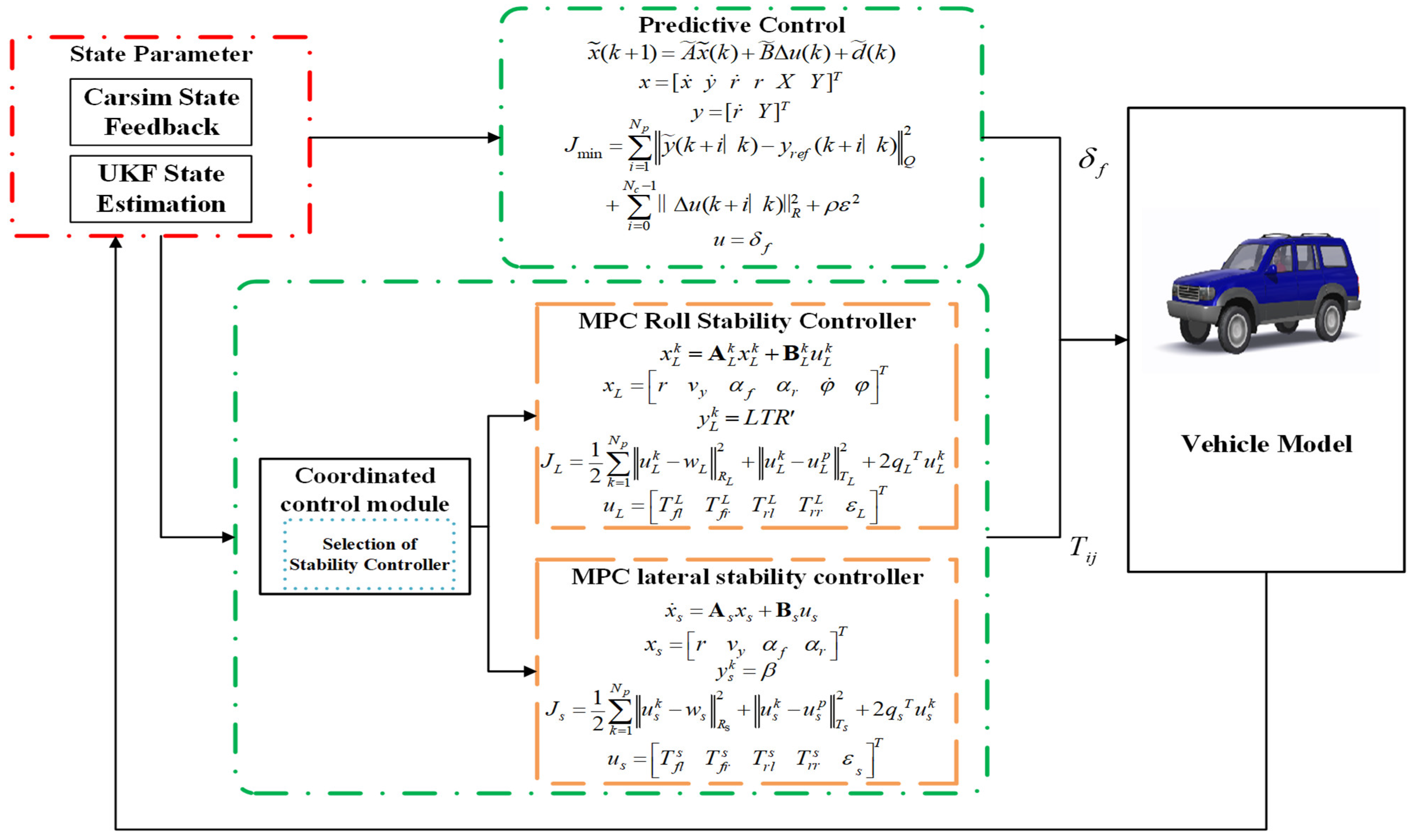
As described in this section, the path tracking stability controller is designed using a hierarchical integrated control structure. The specific composition of the integrated controller is shown in Figure 4.
The two green virtual frames shown in 
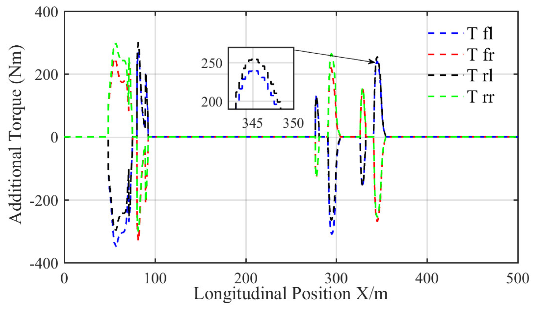
Figure 4 represent the MPC path tracking controller and the MPC stability integrated controller. The stability integrated controller monitors the lateral load transfer rate and the side-slip coefficient in real time through a coordinated control module. According to the internal coordination strategy, the MPC roll stability controller and the MPC lateral stability controller can be used to control the vehicle stability during the path tracking by generating additional torque. The red virtual box represents the state parameter input and output modules; this is used for the closed-loop control of the entire control system. Notably, the coordinated control module is the key to the design of the stability integrated controller, and directly affects the rationality of the control system and accuracy of the control. The coordinated control module includes the selection of the judgment conditions for the vehicle stability and the formulation of the coordination strategies.
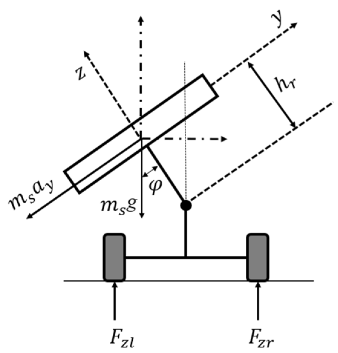
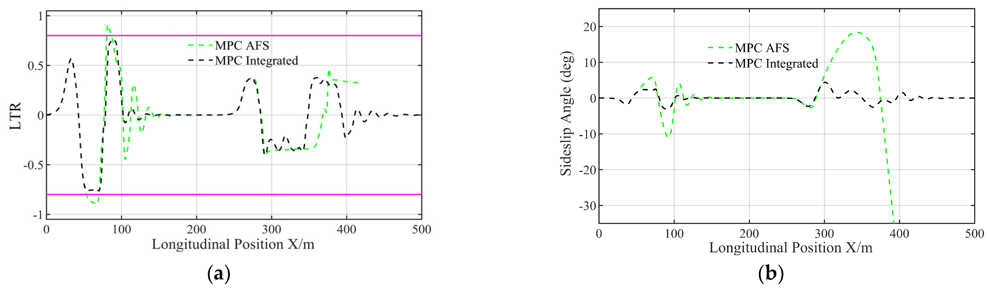
The load transfer ratio (LTR) is often used as a criterion for describing the vehicle rollover stability, and its value directly reflects the vehicle rollover risk. It can be described as follows:
L T R = F z l F z r F z l + F z r - 1 , 1 .
The LTR varies from −1 to 1, where −1 and 1 indicates that the vehicle rolls over. Considering that the vertical load of the wheel is not easy to measure in practice, a state value obtained by a vehicle-mounted sensor or the state estimator is used instead of the vertical load for the approximate calculation of the LTR. The approximate expression is written follows:
L T R 2 h r l e ( sin φ + a y cos φ / g ) ,
where h r is the distance from the center of the roll of the vehicle to the center of mass, l e is the distance between the vehicle suspension springs, g is the gravitational acceleration, and φ is the roll angle.
The lateral sliding coefficient ( ρ ) is the standard for describing the lateral stability of vehicles, and its value directly reflects the risk of the lateral vehicle sliding. It can be described as follows:
ρ = F y F z ,
where F y is the lateral force of the tire and F z is the vertical force of the tire.
As the above two coefficients reflect the stability of the vehicle, in this study, the sideslip coefficient ( ρ ) and lateral LTR are selected as the judgment conditions for the vehicle stability.
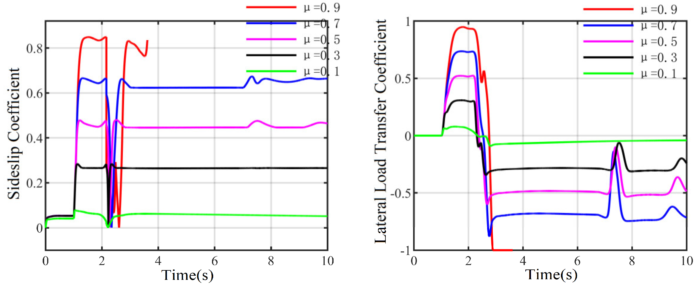
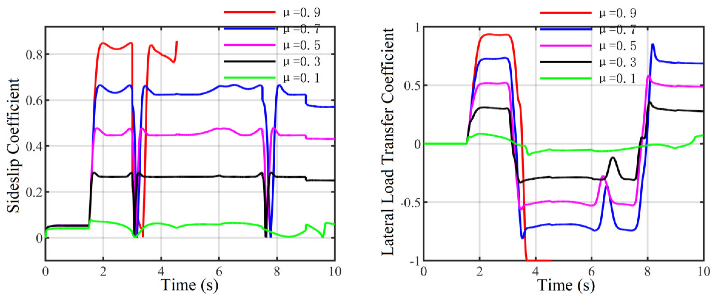
To determine the threshold ranges for the vehicle stability conditions and establish a suitable coordination strategy, the fishhook steering and the snake steering are selected as the test conditions, and the relationship diagram of the road adhesion coefficient ρ and the LTR is drawn. As shown in Figure 5 and Figure 6, the LTR and ρ vary with the steering wheel angle. When the vehicle is under the fishhook or snake condition on a road with an adhesion coefficient of 0.9, a rollover occurs; the LTR reaches 1, and the maximum ρ is approximately 0.83. When a road with an adhesion coefficient of 0.7 undergoes the same steering, the LTR under the fishhook condition reaches 0.88 and that under the snake condition reaches 0.8, whereas the maximum sideslip coefficients under these conditions are 0.63 and 0.65, respectively. When driving on a road with an. adhesion coefficient of 0.5, the maximum value of the LTR under the fishhook condition is approximately 0.52, whereas that under the snake condition is approximately 0.5, and the maximum values of ρ are approximately 0.44 and 0.45, respectively. This indicates that the vehicle is more prone to a plane sideslip instability when performing under high-speed sharp turn conditions on a road with this adhesion coefficient. When the adhesion coefficient is 0.3, the maximum value of the LTR is approximately 0.3 and the maximum value of ρ is 0.25 under the different working conditions.
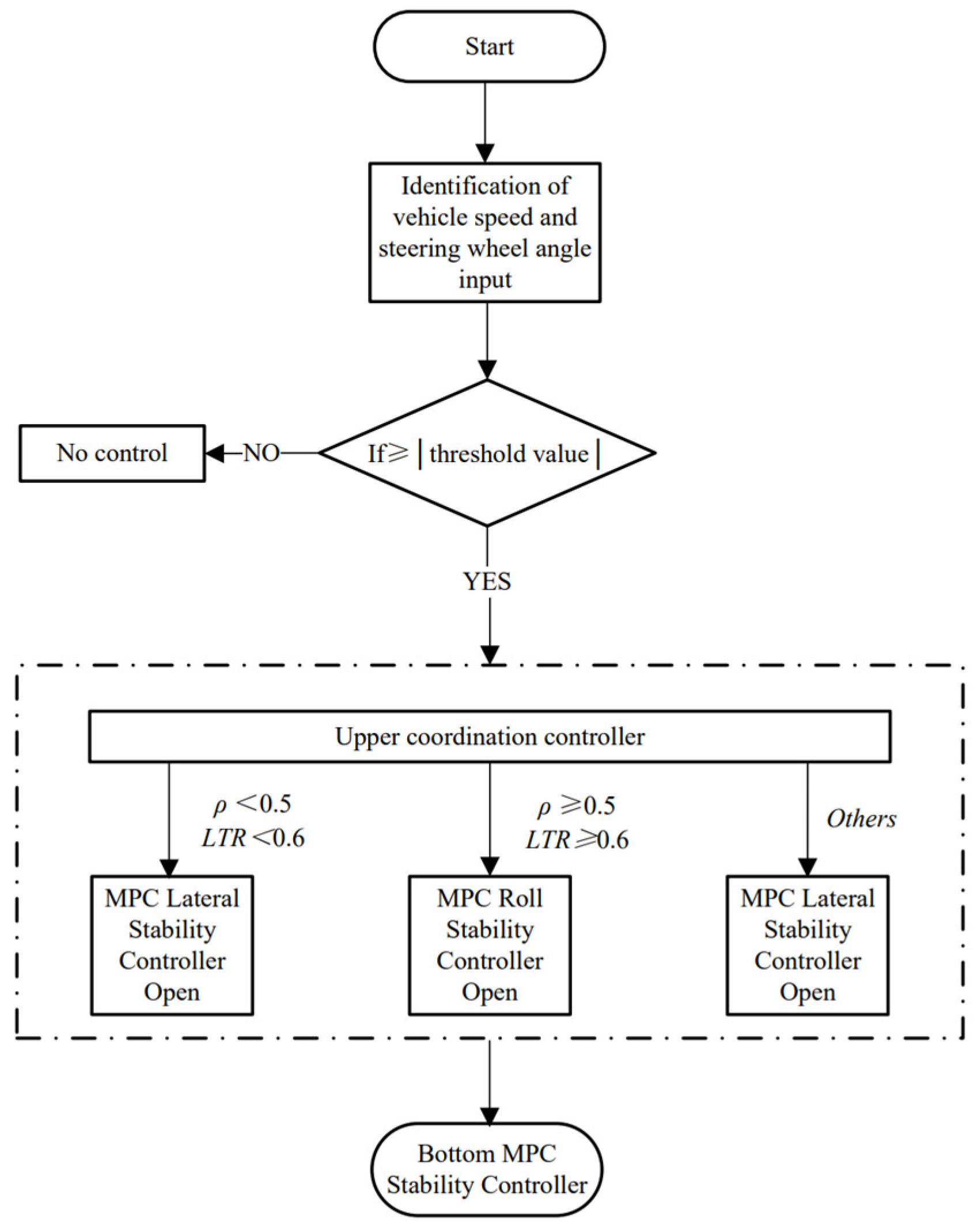
By setting different speeds and steering wheel angles, multiple sets of simulation tests were conducted to determine the threshold intervals for the decision conditions of the LTR and ρ . A coordination strategy was formulated as in Figure 7.
(1) When the vehicle speed and the steering wheel angle are lower than the set thresholds, it indicates that the vehicle is in a safe driving state, and the MPC lateral stability controller and MPC roll stability controller will not be operated.
(2) When the vehicle speed and steering wheel angle exceed the set thresholds, the upper supervision decision module will monitor the lateral LTR and ρ in real time. When the ρ is less than 0.5 and the LTR is less than 0.6, the vehicle is prone to a lateral slip instability when driving on a low-adhesion-coefficient road, but only the MPC lateral stability controller is needed.
(3) When ρ is greater than or equal to 0.5 and the LTR is greater than or equal to 0.6, it indicates that the vehicle driving on the road with a high adhesion coefficient is prone to a rollover instability under the condition of a high-speed sharp turn; accordingly, the MPC roll stability controller is turned on.
(4) Considering that the determination conditions may be in other threshold ranges, such as when ρ is greater than 0.5 and the LTR is less than 0.6, the MPC lateral stability controller is set to be operated.

4.1. Design of the Path Tracking Controller

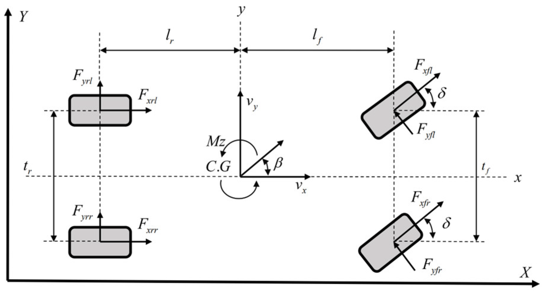
According to the established nonlinear dynamic Equations (1)–(4), a nonlinear state equation can be constructed as follows:
x ˙ ( t ) = f ( x ( t ) , u ( t ) ) ,
where x ( t ) is the state parameter and u ( t ) is the control variable. The specific parameters are as follows:
x ( t ) = [ x ˙   y ˙   r ˙   r   X   Y ] T , u ( t ) = δ f .
A nonlinear MPC path tracking controller can be designed using the nonlinear state equation. Although the control precision can be improved, the nonlinear control method requires a large amount of calculation and may be unable to meet the real-time requirements of the vehicle path tracking under different working conditions. As such, the advantages of the simple calculations and good real-time performance of a linear control method should be considered. Therefore, in view of the above problems, we linearize the nonlinear state equation and use the linearization control method to design the path tracking controller.
Equation (25) can be linearized by using a Taylor expansion at the selecting point ( x 0 ( t ) , u 0 ( t - 1 ) ) . The linearized expression is described as follows.
x ^ ˙ = f ( x ^ , u ^ )
Equation (26) is a continuous equation. As the MPC is a discrete-time control method, (26) can be discretized using the forward Euler method. The discrete state-space expression is written as follows:
x ( k + 1 ) = x ^ ( k + 1 ) + A ( x ( k ) - x ^ ( k ) ) + B ( u ( k ) - u ^ ( k ) ) .
Equation (27) can be expressed as follows:
x ( k + 1 ) = A x ( k ) + B u ( k ) + d ( k ) ,
where I is a unit matrix of the same order as matrix A and T is the sampling period.
d ( k ) = x ^ ( k + 1 ) A x ^ ( k ) B u ^ ( k )
Considering that the control variable may exceed this limit, the control increments in each sampling period are constrained. Equation (28) can be converted to a new state equation containing the control variable Δ u k as follows:
x ˜ ( k + 1 ) = A ˜ x ˜ ( k ) + B ˜ Δ u ( k ) + d ˜ ( k ) ,
where m is the dimension of the control and n is the dimension of the state variables.
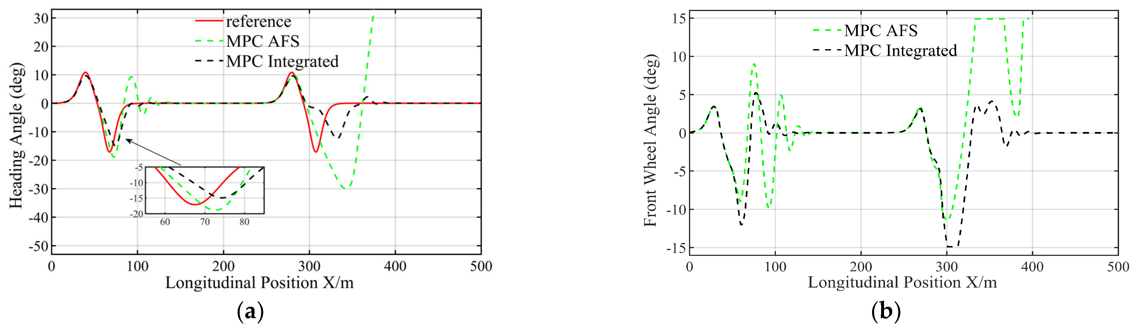
When the vehicle tracks the reference path, the vehicle path tracking accuracy and the lateral stability must be considered. Therefore, the heading angle r and the lateral position Y are used as the outputs of the state space, and the predicted output equation is described as follows:
y ˜ ( k ) = C ˜ x ˜ ( k ) ,
The state-space expression is obtained as follows:
x ˜ ( k + 1 ) = A ˜ x ˜ ( k ) + B ˜ Δ u ( k ) + d ˜ ( k ) y ˜ ( k ) = C ˜ x ˜ ( k ) .
The predictive output equation at time k + 1 is obtained as follows:
y ˜ ( k + 1 ) = C ˜ x ˜ ( k + 1 ) .
Then
y ˜ ( k + 1 ) = C ˜ A ˜ x ˜ ( k ) + C ˜ B ˜ Δ u ( k ) + C ˜ d ˜ ( k ) .
Similarly, the predictive output equation at time [ k , k + N p ] can be obtained. The derived prediction output equation can then be written in the matrix form. Finally, the prediction output expression for the discrete state is obtained as follows:
Y o u t   ( k ) = Ω ( k ) x ˜ ( k ) + Θ ( k ) Δ U ( k ) + Λ ( k ) D ( k ) .
According to (34), the values of r ˙ and the lateral position Y in the predicted time domain can be calculated and applied to the subsequent calculations of the control algorithm.
To ensure that the FWID EV tracks the desired path smoothly and rapidly, an optimal control variable is generated by obtaining the minimum value of the defined objective function. The objective function is defined as follows:
J min ( x ˜ ( k ) , u ( k 1 ) , Δ u ( k ) , ε ) = i = 1 N p y ˜ ( k + i k ) y r e f ( k + i k ) Q 2 + i = 0 N c 1 Δ u ( k + i k ) R 2 + ρ ε 2 ,
where N p and N c are the prediction and control time domains, respectively, Q is the output weighting matrix, R is the control weighting matrix, ρ is the weight coefficient, and ε is a relaxation factor. The first item of the objective function reflects the fast tracking ability of the control system for the desired path. The second item reflects the requirements of the control system for the stable changes in the control variable. Considering the real-time changes in the control system, the optimal solution of the objective function in each control period cannot be guaranteed. When there is no optimal solution, the relaxation factor is added to the objective function, and the control system can replace the optimal solution with a suboptimal solution to avoid the occurrence of no solution.
Considering that an actual vehicle steering actuator has a certain scope of work, to avoid the controller producing a front wheel angle beyond the working range, it is also necessary to constrain the control variable and control increment generated by the controller. The constraints are as follows.
U min ( k ) U ( k ) U max ( k )
Δ U min ( k ) Δ U ( k ) Δ U max ( k )
Moreover, the prediction output must be constrained, and the constraint is set as follows:
Y o u t min ( k ) Ω ( k ) x ˜ ( k ) + Θ ( k ) Δ U ( k ) + Λ ( k ) D ( k ) Y o u t max ( k ) .
To facilitate the controller programming to solve for the optimal control variable, it is necessary to convert the general objective function into a quadratic programming (QP) problem.
J = Y o u t   ( k ) Y r e f   ( k ) T Q Y o u t   ( k ) Y r e f   ( k ) + Δ U ( k ) T R Δ U ( k ) + ρ ε 2 ,
E ( k ) = Y r e f ( k ) Ω ( k ) x ˜ ( k ) Λ ( k ) D ( k ) .
Then,
J = 1 2 ξ ( k ) T H ( k ) ξ ( k ) + f ( k ) ξ ( k ) ,
Finally, for each sampling period, the optimization problems with constraints are solved and a control increment sequence in the N p range can be obtained as follows:
U ( k ) = Δ u ( k |   k ) Δ u ( k + 1 |   k )     Δ u ( k + N c 1 |   k ) .
As the MPC algorithm selects the first control increment Δ u ( k |   k ) from the control increment sequence, the optimal control variable acting on the vehicle path tracking at the current moment is expressed as follows:
u ( k |   k ) = u ( k 1 |   k ) + Δ u ( k |   k ) .
Similarly, the control system repeats the above steps at time k + 1, and ultimately obtains the optimal front wheel angle for tracking the expected path.

4.2. Design of the Vehicle Roll Stability Controller

Based on the MPC theory [31] and the vehicle dynamics equations, the nonlinear state equation is established as follows:
x ˙ L = A L x L + B L u L   ,
where x L is the state variable and u L is the control variable. The specific parameters are as follows:
x L = [ r   v y   α f   α r   φ ˙   φ ] T , u L = [ T f l L   T f r L   T r l L   T r r L   ε L ] T .
These equations are then combined in the matrix form to obtain the predictive output expression for the discrete state as follows:
y ¯ L k = Ω L k x ¯ L k + Θ L k u ¯ L k .
The specific objective function is designed as follows:
J L = 1 2 k = 1 N p u L k w L R L 2 + u L k u L p T L 2 + 2 q L T u L k   ,
where
w L = T f l L d T f r L d T r l L d T r r L d 0 T ,   q L = 0 0 0 0 r   L 1 ε T .
In the above equation, T L = diag t L T   t L T   t L T   t L T   t L ε , R L = diag r L T   r L T   r L T   r L T   r   L 2 ε , where u L k is the expected additional torque generated by the controller on the four wheels. The T i j L d in W L is the driver-input four-wheel-drive torque, and its role is to maintain a certain speed. u L P is the last control variable solved for by the controller. T L and R L are the weight matrices. t L T is the weight of the control increment of the roll stability controller, r L T is the weight of the control variable of the roll stability controller, and r L 1 ε and r L 2 ε are the weights of the relevant relaxation factors. The objective function is divided into three functions. The first function ensures that when the controller detects a control target value greater than the set threshold, the controller generates an additional torque. The second function ensures steady changes in the control quantity and avoids large oscillations which would otherwise affect the normal operation of the vehicle. The job of the third function is to avoid a “no solution” situation of the controller.
To facilitate programming, the general objective function in (46) is converted into a standard QP form. The specific expressions are as follows:
J L = 1 2 u L k ¯ T ( R L ¯ + T L ¯ ) u L k ¯ + u L k ¯ q L ¯ T w L ¯ T R L ¯ u L P ¯ T T L ¯ T ,
Finally, the constraint conditions are designed. To provide the roll stability for the vehicle under the conditions of high speed and sharp rotation, the approximate vertical load coefficient L T R of the vehicle is constrained. The constraint equation is as follows:
y L k L T R max + ε L ,
where L T R max is the vertical load threshold, which is set to 0.8.
In the control process, to avoid the control amount calculated by the controller from exceeding the maximum control amount that can be generated by the motor, the control variables need to be constrained. The constraint expression for the control variables is defined as follows:
l b u L u b 0 ε L ,
where l b = [ T min L   0 ] T , u b = [ T max L + ] T , and T min L and T max L are the minimum and maximum additional torque values, respectively.
The above constraint expression only imposes upper and lower bounds on the output variable and the control variables at a single time. To obtain the optimal control sequence of the objective function, it is necessary to restrict the output and the control variables of the [ k , k + N p ] -time prediction model. At time [ k , k + N p ] , the matrix of the constraint expression is reorganized, and expressions are obtained as follows:
L B < u ¯ L < U B A u u ¯ L < U B u .

4.3. Design of the Vehicle Lateral Stability Controller

In this section, the vehicle lateral stability controller is designed based on the roll stability controller. For the prediction model, the design of the objective function and the constraint conditions and the specific meaning of the parameters in each expression are similar. Therefore, this section introduces the design of the lateral stability controller.
The nonlinear state equations are established as follows:
x ˙ s = A s x s + B s u s   .
Equation (51) is linearized to obtain the linearized state equation as follows:
x ˙ s t = A s t x s t + B s t u s t ,
In addition, (52) is discretized as follows:
x s k + 1 = A s k x s k + B s k u s k ,
The vehicle lateral velocity is selected as the output, and is expressed as follows:
y s k = C S x s k .
The value at time [ k , k + N p ] is restructured to obtain the predictive output expression of the discrete state as follows:
y ¯ s k = Ω s k x ¯ s k + Θ s k u ¯ s k ,
The objective function of the lateral stability controller is designed as follows:
J s = 1 2 k = 1 N p u s k w s 2 R S + u s k u s p 2 T S + 2 q s T u s k   .
The objective function in (56) can be converted into a standard QP form as
J L = 1 2 u s k ¯ T ( R s ¯ + T s ¯ ) u s k ¯ + u s k ¯ q s ¯ T w s ¯ T R s ¯ u s P ¯ T T s ¯ T .
The specific meanings of each variable are consistent with those of the roll-stability controller. To provide driving stability to the vehicle on a low-attachment road, the sideslip angle of the vehicle can be expressed as follows
y s k β max + ε s .
In this study, the roll and lateral stability controllers are designed for the same vehicle type; therefore, the constraint design for the stability controller control quantity is consistent with that for the roll stability controller.

5. Simulation Results

5.1. Simulation Verification 1

The initial velocity was 80 km/h, and a docking pavement was set. The road adhesion coefficient at the longitudinal positions in the 0–200 m range was set to 0.85, whereas that at the longitudinal positions in the 200–500 m range was set to 0.35. The specific simulation results are shown below.
A comparison graph between the actual and reference paths is shown in Figure 8. As shown in the figure, the control effects of the MPC path tracking controller (MPC AFS) and the path tracking stability controller (MPC Integrated) are compared. When the vehicle runs on a road with a high adhesion coefficient at a speed of 80 km/h, the real-time and accurate tracking of the desired path is realized under the action of the MPC AFS controller and the MPC Integrated controller. When the vehicle enters the low-adhesion-coefficient road, the actual path deviates significantly from the expected path under the action of the MPC AFS controller, and the path tracking fails. Under the action of the MPC Integrated controller, although the actual path deviates from the expected path to a certain extent when the road curvature changes significantly, the actual path quickly converges to the expected path.
A comparison graph between the heading angle and front wheel angle is shown in Figure 9 and that between the longitudinal velocity and the yaw rate is shown in Figure 10. As shown in Figure 9 and Figure 10, when the vehicle with the MPC AFS controller tracks the path on the road with a high adhesion coefficient, the heading angle, the front wheel angle, and the yaw rate oscillate significantly at approximately 90 m in the longitudinal position, and the vehicle might be under the danger of instability. When the vehicle tracks the path on the road with an adhesion coefficient of 0.35, the three state variables show monotonic changes and the longitudinal speed begins to decline rapidly, indicating that the vehicle had a serious sideslip. When the vehicle uses the MPC Integrated controller to track the path on the docking road at medium and high speeds, there are no significant oscillations in the heading and front wheel angles. Simultaneously, the longitudinal vehicle speed changes smoothly and the yaw rate is controlled within a safe range.
A comparison graph between the lateral load transfer coefficient and the sideslip angle of the centroid is shown in Figure 11. As shown in Figure 11, compared with the MPC AFS controller, the MPC Integrated controller ensures the safety and stability of the vehicle when tracking a double lane-change path on the docking road. The lateral load transfer rate and the sideslip angle of the centroid are effectively limited to a reasonable range, and the maximum sideslip angle of the centroid is approximately 4°.
The additional torque of the path tracking stability controller is illustrated in Figure 12. As shown in Figure 12, with the input of the front wheel angle, the MPC Integrated controller can quickly generate an additional torque to adjust the stable state of the vehicle. Moreover, the action time is short, and therefore, it will not have an excessive influence on the path tracking effect owing to the excessive application of the additional torque.

5.2. Simulation Verification 2

Based on simulation experiment 1, a higher initial velocity (110 km/h) was set to further verify the effect of the controller, and the other simulation conditions were set to the same values as those in simulation experiment 1. The analysis of the simulation results is as follows.
A comparison graph between the actual and reference paths is shown in Figure 13. As shown in Figure 13, the MPC AFS controller cannot maintain the stability of the high-speed path tracking under the different working conditions, and in the first half of the simulation test, the actual path significantly deviates from the desired path. Compared with the MPC AFS controller, the MPC Integrated controller realizes the vehicle path tracking on a high-adhesion road; however, when the vehicle enters a low-adhesion road and performs a large steering angle for a large change in a road curvature, the front wheel inevitably reaches a lateral saturation, and the tracking of the desired path deviates. However, under the action of the MPC Integrated controller, the expected path is tracked as far as possible in the latter half of the simulation, under the premise of ensuring the stability of the vehicle.
A comparison graph between the heading and front wheel angles is shown in Figure 14 and that between the longitudinal velocity and the yaw rate is shown in Figure 15. It can be seen from Figure 14 and Figure 15 that when the vehicle is on a road with a high adhesion coefficient, the monotonic changes in the heading angle, the front wheel angle, the longitudinal velocity, and the yaw rate occur owing to the instability of the vehicle, and they are significantly beyond the stability critical value range. Under the action of the MPC Integrated controller, when the vehicle is tracked on roads with different adhesion coefficients, the longitudinal speed changes smoothly and is stable between 100 and 110 km/h. In addition, the yaw rate and the front wheel angle change trends are relatively stable. The actual heading angle deviates from the expected heading angle in the latter half of the simulation, and the expected heading angle is re-tracked at approximately 420 m in the longitudinal position. This phenomenon is also reflected in the comparison between the actual and expected paths.
A comparison graph between the lateral load transfer coefficient and the sideslip angle of the centroid is shown in Figure 16. As shown in Figure 16, under the action of the MPC Integrated controller, the stability of the vehicle path tracking at higher speeds is ensured. The maximum lateral load transfer rate is approximately 0.79, and the sideslip angle is controlled within a stable range.
An additional torque graph of the path tracking stability controller is shown in Figure 17. In Figure 17, when the initial speed is set to 110 km/h, the MPC Integrated controller needs to generate greater additional torque to maintain the stability of the vehicle because the dynamic state parameters of the vehicle change significantly. Simultaneously, the change in the additional torque is relatively stable, providing a guarantee for tracking the desired path after the vehicle resumes stable driving.
From the above two simulation experiments, it can be seen that under the action of the MPC Integrated controller, the lateral load transfer rate and the sideslip angle of the vehicle during the high-speed path tracking are effectively reduced, ensuring the driving stability of the vehicle and improving the path tracking performance.

6. Conclusions

Looking at the problems of tracking failures and vehicle instability in FWID EVs path tracking under extreme conditions, a path tracking stability controller is designed based on a hierarchical integrated control structure. Compared with a single path tracking controller, the proposed controller displays a better control effect and stronger stability under extreme conditions. The simulation results show that the path tracking stability controller designed in this study reduces the lateral load transfer rate and the centroid sideslip angle of the vehicle during the high-speed path tracking. Simultaneously, it also ensures the driving stability of the vehicle and improves the path tracking performance.

Author Contributions

Conceptualization and supervision, H.J.; conception and design, Y.X. and C.L.; manuscript writing, W.A. and J.Q. All authors have read and agreed to the published version of the manuscript.

Funding

This work was partially supported by the National Natural Science Foundation of China (52262052) and the Natural Science Foundation of Guangxi Province (2020GXNSFAA297031).

Institutional Review Board Statement

Not applicable.

Informed Consent Statement

Not applicable.

Data Availability Statement

Not applicable.

Conflicts of Interest

The authors declare no conflict of interest.

References

  1. Jin, X.; Wang, J.; Yan, Z. Robust vibration control for active suspension system of in-wheel-motor-driven electric vehicle via μ-synthesis methodology. J. Dyn. Syst. Meas. Control. 2022, 144, 051007. [Google Scholar] [CrossRef]
  2. Deng, Z.; Li, X.; Liu, T. Modeling and suppression of unbalanced radial force for in-wheel motor driving system. J. Vib. Control. 2021, 1–12. [Google Scholar] [CrossRef]
  3. Wang, Z.; Zha, J.; Wang, J. Autonomous vehicle trajectory following: A flatness model predictive control approach with hardware-in-the-loop verification. IEEE Trans. Intell. Transp. Syst. 2020, 22, 5613–5623. [Google Scholar] [CrossRef]
  4. Wang, Z.; Bai, Y.; Wang, J.; Wang, X. Vehicle path tracking LTV-MPC controller parameter selection considering CPU computational load. ASME Trans. J. Dyn. Syst. Meas. Control. 2019, 141, 051004-1. [Google Scholar] [CrossRef]
  5. Jin, X.; Yang, J.; Li, Y.; Zhu, B.; Wang, J.; Yin, G. Online estimation of inertial parameter for lightweight electric vehicle using dual unscented Kalman filter approach. IET Intel. Trans. Syst. 2020, 14, 412–422. [Google Scholar] [CrossRef]
  6. Shi, K.; Yuan, X.; Huang, G. Compensation-based robust decoupling control system for the lateral and longitudinal stability of distributed drive electric vehicle. IEEE/ASME Trans. Mechatron. 2019, 24, 2768–2778. [Google Scholar] [CrossRef]
  7. Zhang, H.; Wang, J. Vehicle lateral dynamics control through AFS/DYC and robust gain-scheduling approach. IEEE Trans. Veh. Technol. 2015, 65, 489–494. [Google Scholar] [CrossRef]
  8. Takahashi, J.; Yamakado, M.; Saito, S. A hybrid stability-control system: Combining direct-yaw-moment control and G-Vectoring control. Veh. Syst. Dyn. 2012, 50, 847–859. [Google Scholar] [CrossRef]
  9. Shuai, Z.; Zhang, H.; Wang, J. Combined AFS and DYC control of four-wheel-independent-drive electric vehicles over CAN network with time-varying delays. IEEE Trans. Veh. Technol. 2013, 63, 591–602. [Google Scholar] [CrossRef]
  10. Huang, G.; Yuan, X.; Shi, K. A BP-PID controller-based multi-model control system for lateral stability of distributed drive electric vehicle. J. Frankl. Inst. 2019, 356, 7290–7311. [Google Scholar] [CrossRef]
  11. Tian, Y.; Yao, Q.; Wang, C. Switched model predictive controller for path tracking of autonomous vehicle considering rollover stability. Veh. Syst. Dyn. 2021, 1–20. [Google Scholar] [CrossRef]
  12. Magalhães, Z.R., Jr.; De Almeida, A.M.; Lopes, R.V. Vehicle stability upper-level-controller based on parameterized model predictive control. IEEE Access. 2022, 10, 21048–21065. [Google Scholar] [CrossRef]
  13. Hu, C.; Wang, Z.; Qin, Y. Lane keeping control of autonomous vehicles with prescribed performance considering the rollover prevention and input saturation. IEEE Trans. Intel. Trans. Syst. 2019, 21, 3091–3103. [Google Scholar] [CrossRef]
  14. Zhang, X.; Yang, Y.; Guo, K. Contour line of load transfer ratio for vehicle rollover prediction. Veh. Syst. Dyn. 2017, 55, 1748–1763. [Google Scholar] [CrossRef]
  15. Yoon, J.; Cho, W.; Koo, B. Unified chassis control for rollover prevention and lateral stability. IEEE Trans. Veh. Technol. 2008, 58, 596–609. [Google Scholar] [CrossRef]
  16. Shi, K.; Yuan, X.; He, Q. Double-layer dynamic decoupling control system for the yaw stability of four wheel steering vehicle. Int. J. Control. Autom. Syst. 2019, 17, 1255–1263. [Google Scholar] [CrossRef]
  17. Peng, H.; Wang, W.; An, Q. Path tracking and direct yaw moment coordinated control based on robust MPC with the finite time horizon for autonomous independent-drive vehicles. IEEE Trans. Veh. Technol. 2020, 69, 6053–6066. [Google Scholar] [CrossRef]
  18. Hu, C.; Jing, H.; Wang, R. Robust H∞ output-feedback control for path following of autonomous ground vehicles. Mech. Syst. Signal Process. 2016, 70, 414–427. [Google Scholar] [CrossRef]
  19. Liu, J.; Huang, Z.; Xu, X. Multi-Kernel Online Reinforcement Learning for Path Tracking Control of Intelligent Vehicles. IEEE Trans. Syst. Man Cybern. Syst. 2020, 51, 6962–6975. [Google Scholar] [CrossRef]
  20. Liu, Q.; Song, S.; Hu, H. Extended model predictive control scheme for smooth path following of autonomous vehicles. Front. Mech. Eng. 2022, 17, 4. [Google Scholar] [CrossRef]
  21. Guo, H.; Cao, D.; Chen, H. Vehicle dynamic state estimation: State of the art schemes and perspectives. IEEE/CAA J. Autom. Sin. 2018, 5, 418–431. [Google Scholar] [CrossRef]
  22. Fei, J.; Chen, Y. Dynamic Terminal Sliding-Mode Control for Single-Phase Active Power Filter Using New Feedback Recurrent Neural Network. IEEE Trans. Power Electron. 2020, 35, 9904–9922. [Google Scholar] [CrossRef]
  23. Ji, Y.; Jiang, X.; Wan, L. Hierarchical least squares parameter estimation algorithm for two-input Hammerstein finite impulse response systems. J. Franklin I. 2020, 357, 5019–5032. [Google Scholar] [CrossRef]
  24. Cui, R.; Chen, L.; Yang, C. Extended state observer-based integral sliding mode control for an underwater robot with unknown disturbances and uncertain nonlinearities. IEEE Trans. Ind. Electron. 2017, 64, 6785–6795. [Google Scholar] [CrossRef]
  25. Ma, H.; Pan, J.; Ding, F. Partially-coupled least squares based iterative parameter estimation for multi-variable output-error-like autoregressive moving average systems. IET Control Theory Appl. 2019, 13, 3040–3051. [Google Scholar] [CrossRef]
  26. Song, Y.T.; Shu, H.Y.; Chen, X.B. Chassis integrated control for 4WIS distributed drive Evs with model predictive control based on the UKF observer. Sci. China Technol. Sci. 2020, 63, 397–409. [Google Scholar] [CrossRef]
  27. Leung, K.T.; Whidborne, J.F.; Purdy, D. Road vehicle state estimation using low-cost GPS/INS. Mech. Syst. Signal Process. 2011, 25, 1988–2004. [Google Scholar] [CrossRef]
  28. Li, X.; Song, X.; Chan, C. Reliable vehicle sideslip angle fusion estimation using low-cost sensors. Measurement 2014, 51, 241–258. [Google Scholar] [CrossRef]
  29. Hu, G.; Gao, B.; Zhong, Y. Unscented kalman filter with process noise covariance estimation for vehicular INS/GPS integration system. Inf. Fusion. 2020, 64, 194–204. [Google Scholar] [CrossRef]
  30. Jin, X.B.; Robert Jeremiah, R.J.; Su, T.L. The new trend of state estimation: From model-driven to hybrid-driven methods. Sensors 2021, 21, 2085. [Google Scholar] [CrossRef] [PubMed]
  31. Zhang, L.; Chen, H.; Huang, Y. Model predictive control for integrated longitudinal and lateral stability of electric vehicles with in-wheel motors. IET Control Theory Appl. 2020, 14, 2741–2751. [Google Scholar] [CrossRef]
Figure 1. Vehicle planar four-wheel dynamics model.
Machines 10 00859 g001
Figure 2. Vehicle roll dynamics model.
Machines 10 00859 g002
Figure 3. Unscented Kalman filter (UKF) state estimation principle framework.
Machines 10 00859 g003
Figure 4. Path tracking stability control logic diagram.
Machines 10 00859 g004
Figure 5. Comparison of ρ and the load transfer ratio (LTR) under different road adhesion coefficients (Fishhook condition).
Machines 10 00859 g005
Figure 6. Comparison of ρ and the LTR under different road adhesion coefficients (Snake condition).
Machines 10 00859 g006
Figure 7. Coordination strategy flowchart.
Machines 10 00859 g007
Figure 8. Comparison between the actual and reference paths at lower speed ( V x = 80 km / h ).
Machines 10 00859 g008
Figure 9. Comparison of (a) heading angle and (b) front wheel angle at lower speed ( V x = 80 km / h ).
Machines 10 00859 g009
Figure 10. Comparison of (a) longitudinal velocity and (b) yaw rate at lower speed ( V x = 80 km / h ).
Machines 10 00859 g010
Figure 11. Comparison of (a) lateral LTR and (b) sideslip angle of the centroid at lower speed ( V x = 80 km / h ).
Machines 10 00859 g011
Figure 12. Additional torque of the path tracking stability controller at lower speed ( V x = 80 km / h ).
Machines 10 00859 g012
Figure 13. Comparison between the actual and reference paths at higher speed ( V x = 110 km / h ).
Machines 10 00859 g013
Figure 14. Comparison of (a) heading angle and (b) front wheel angle at higher speed ( V x = 110 km / h ).
Machines 10 00859 g014
Figure 15. Comparison of (a) longitudinal velocity and (b) yaw rate at higher speed ( V x = 110 km / h ).
Machines 10 00859 g015
Figure 16. Comparison of (a) lateral LTR and (b) sideslip angle of the centroid at higher speed ( V x = 110 km / h ).
Machines 10 00859 g016
Figure 17. Additional torque of the path tracking stability controller at higher speed ( V x = 110 km / h ).
Machines 10 00859 g017
Publisher’s Note: MDPI stays neutral with regard to jurisdictional claims in published maps and institutional affiliations.

