
A Robust Gaussian Process-Based LiDAR Ground Segmentation Algorithm for Autonomous Driving

 ,
,
Abstract
:1. Introduction
1.1. Background
1.2. Related Work
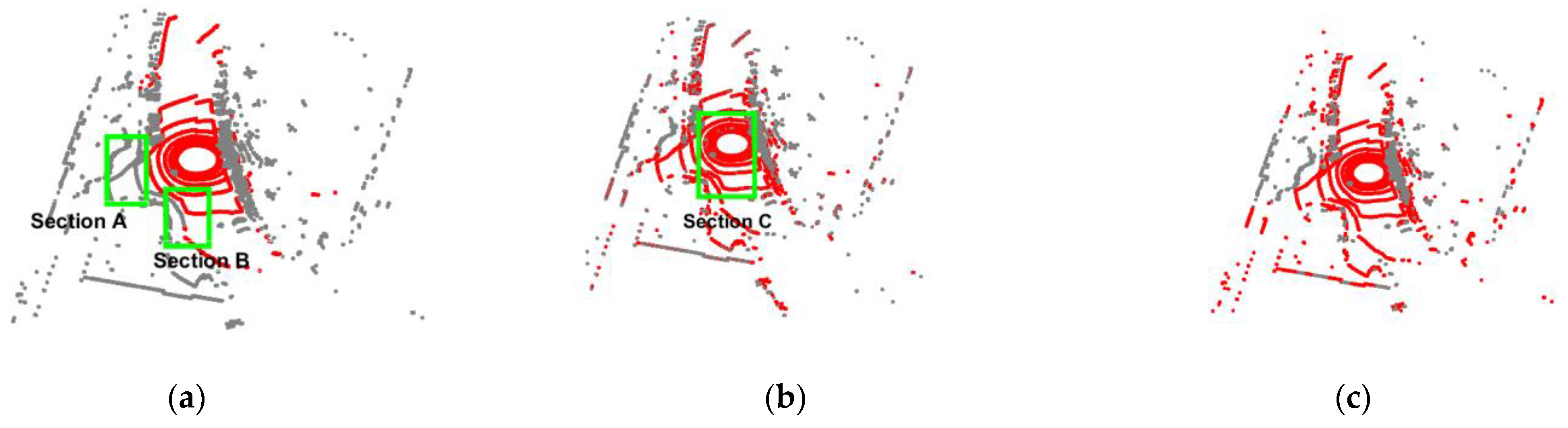
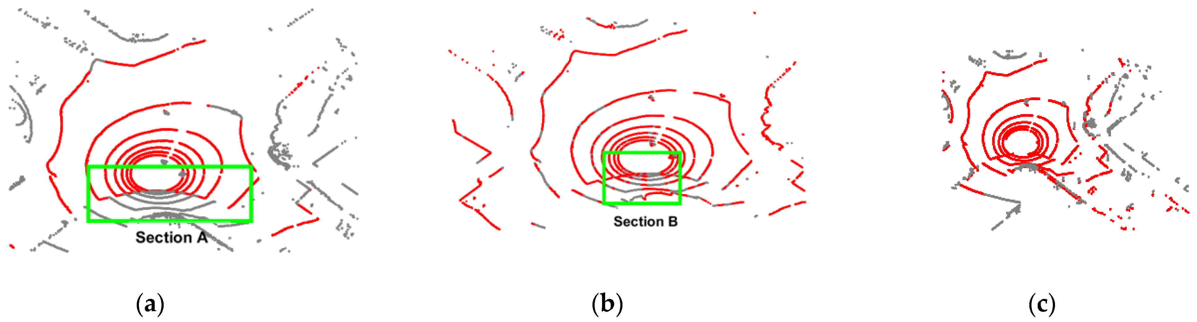
- (a)
- We design height and slope criteria to search for in the initial ground points selection stage. Different from RGF, the proposed algorithm only finds enough ground points for the subsequent training of Gaussian process parameters, so it can have stricter screening conditions. Compared with the RGF algorithm, it can effectively prevent over-segmentation.
- (b)
- We introduce a Gaussian process based on a sparse covariance function for ground reference height estimation. The introduction of sparse covariance makes the description of the ground more reasonable and computationally more efficient.
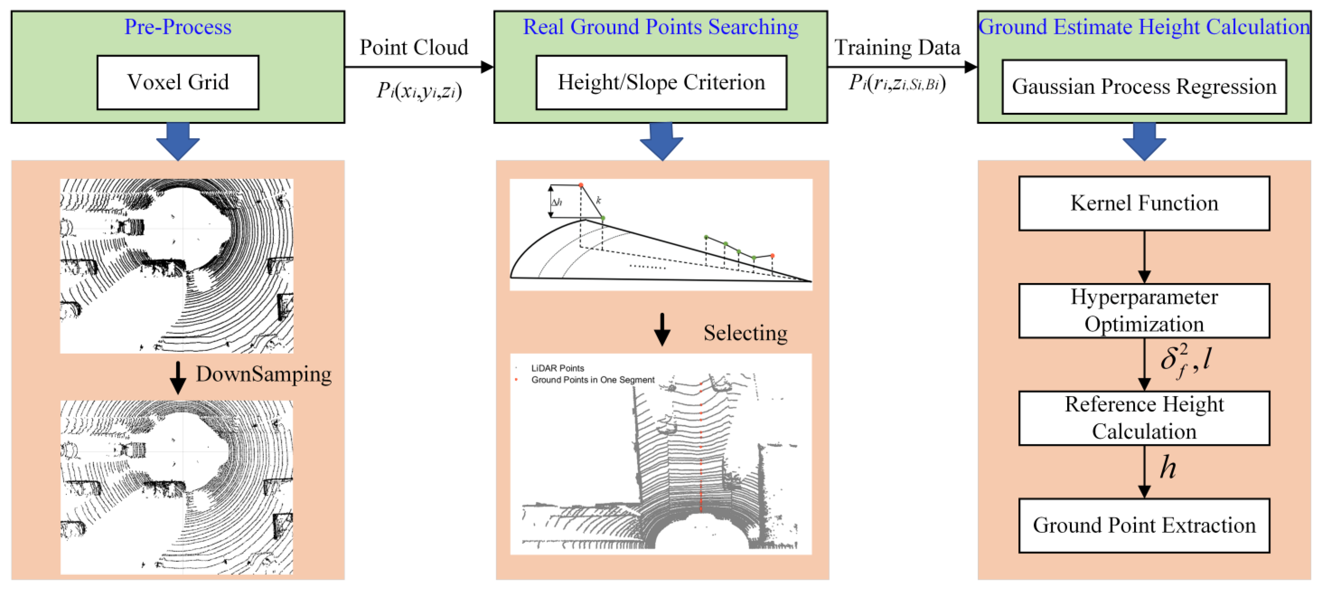
2. Raw Data Pretreatment and Ground Candidate Points Selection
2.1. Raw Point Cloud Downsample
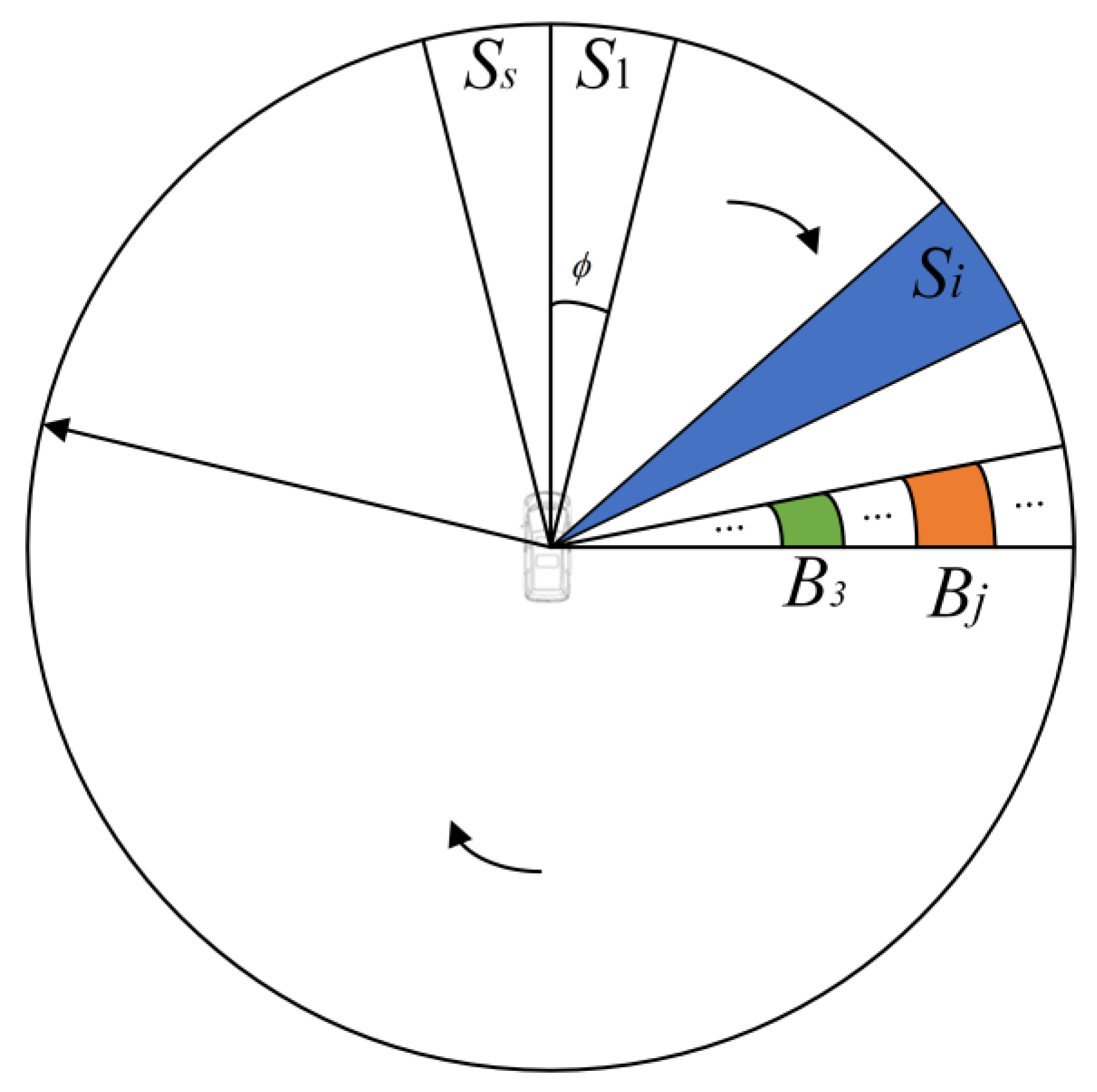
2.2. Point Cloud Coordinate Projection
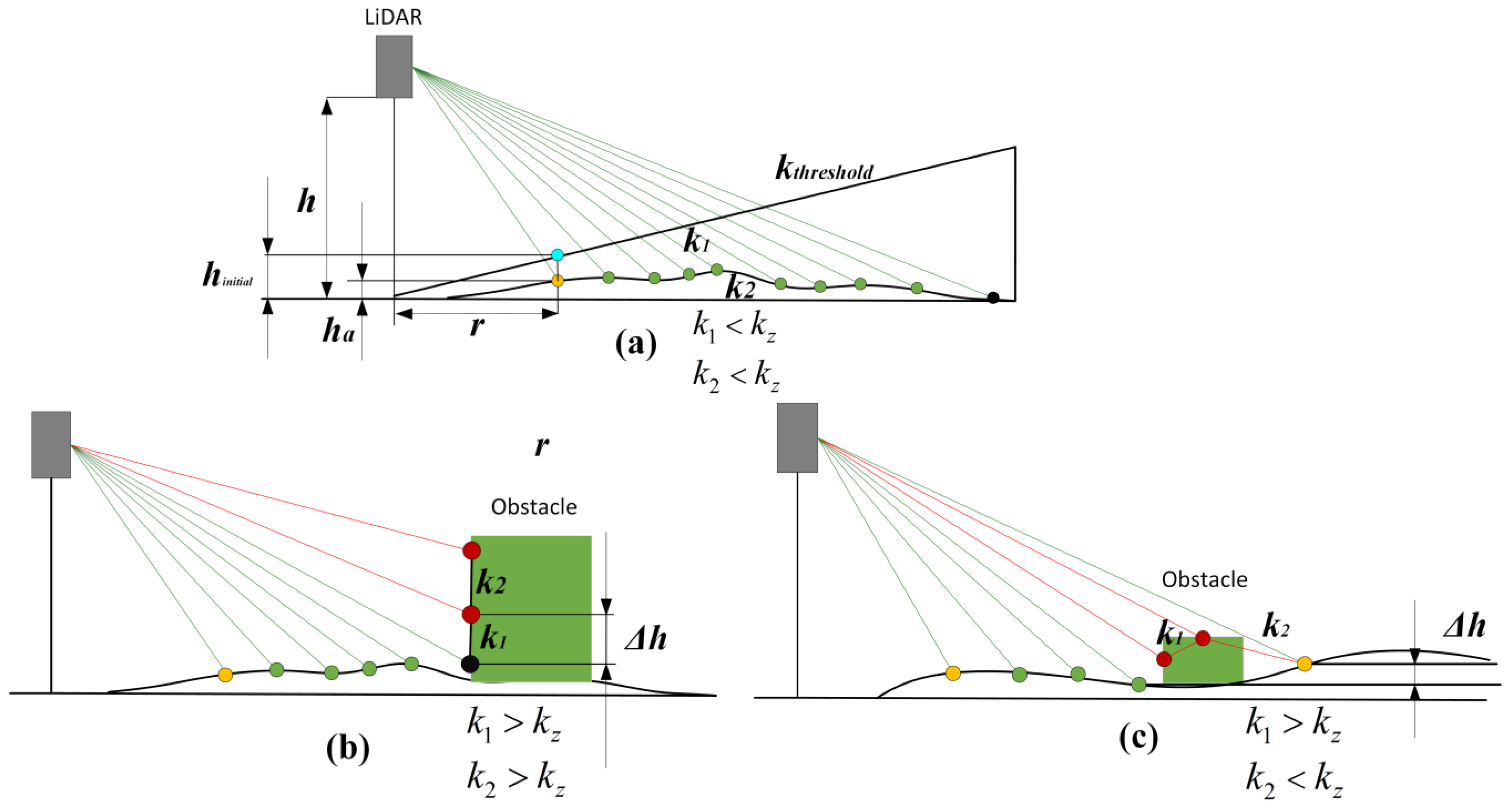
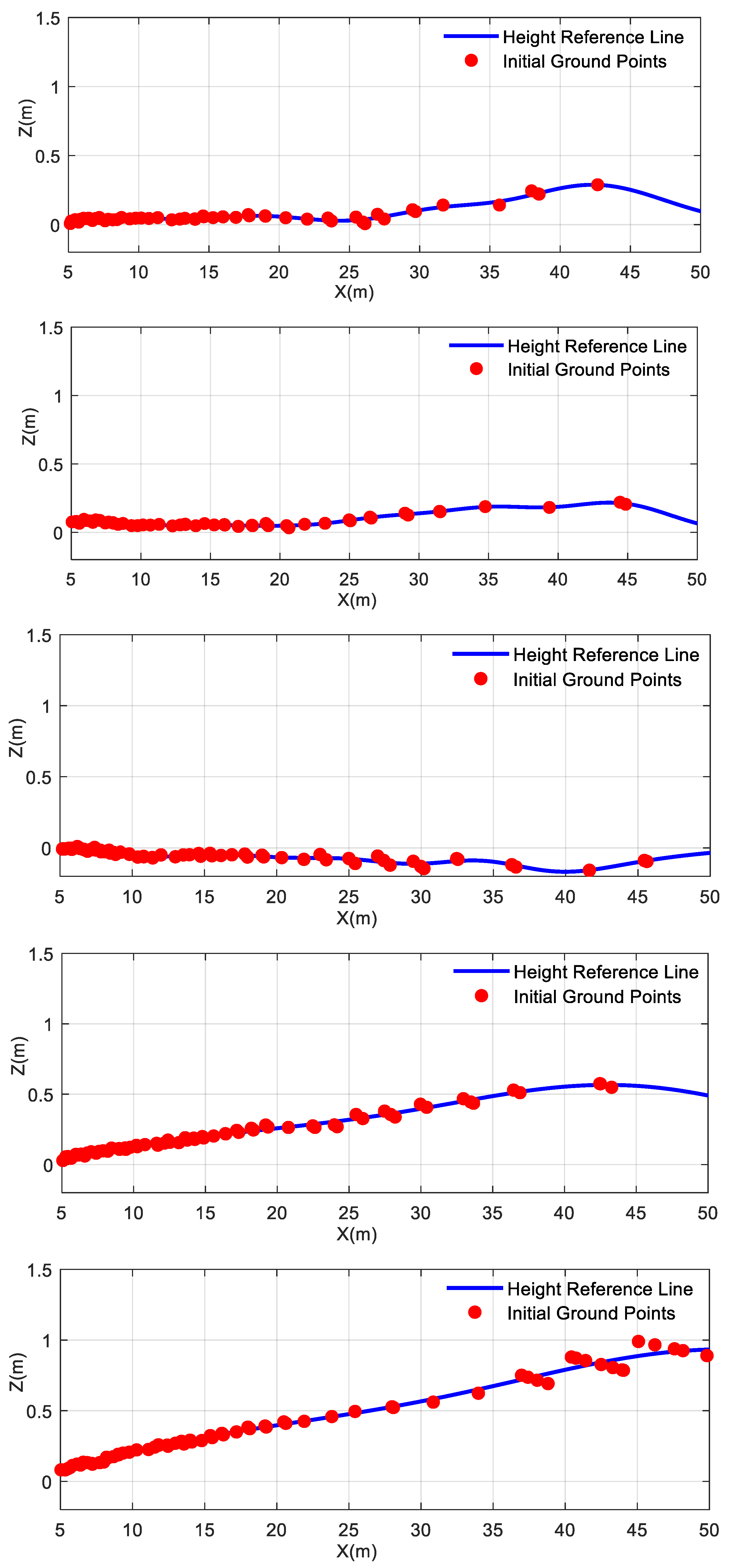
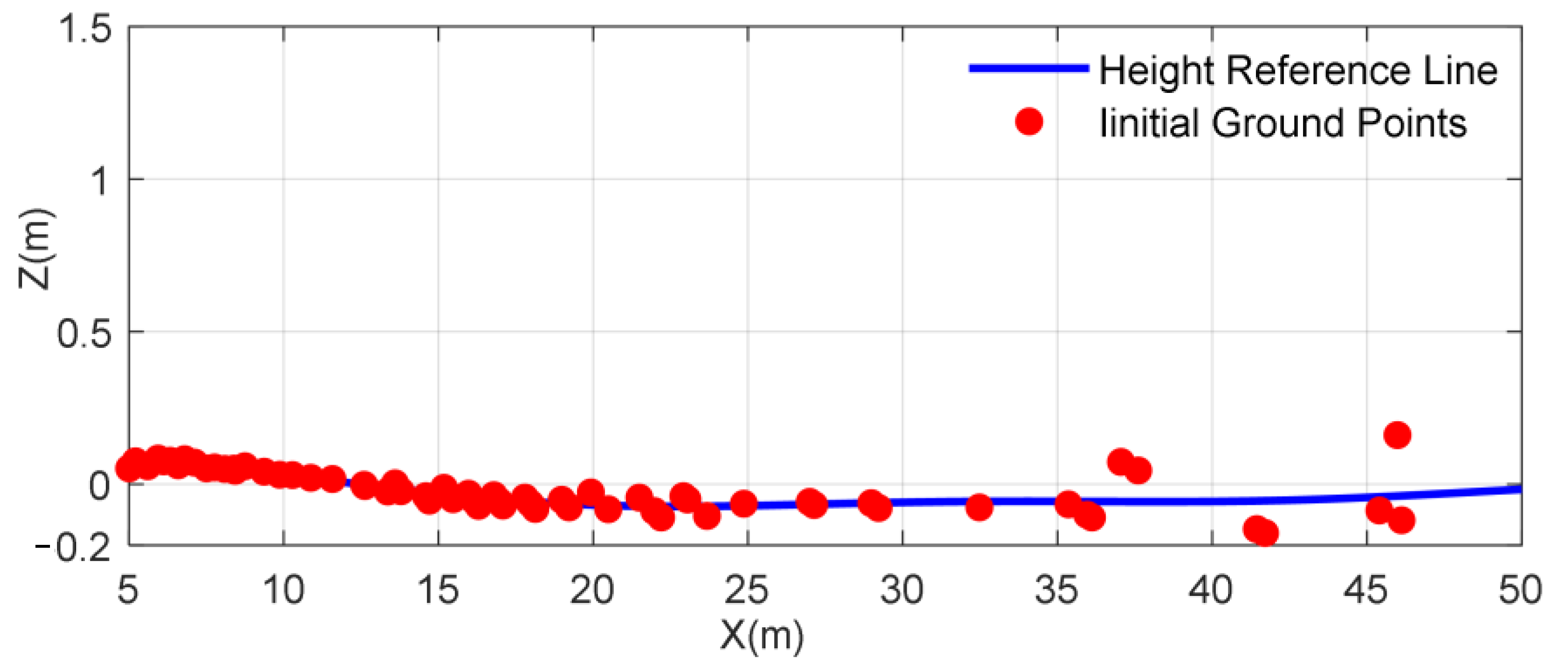
2.3. Ground Candidate Point Selection
3. Gaussian Process Regression Based on Sparse Covariance Function for Ground Segmentation
3.1. Gaussian Process
3.2. Gaussian Process Regression Based on Sparse Kernel Function for Ground Segmentation
| Algorithm1 Ground segmentation based on Gaussian process regression with sparse covariance function |
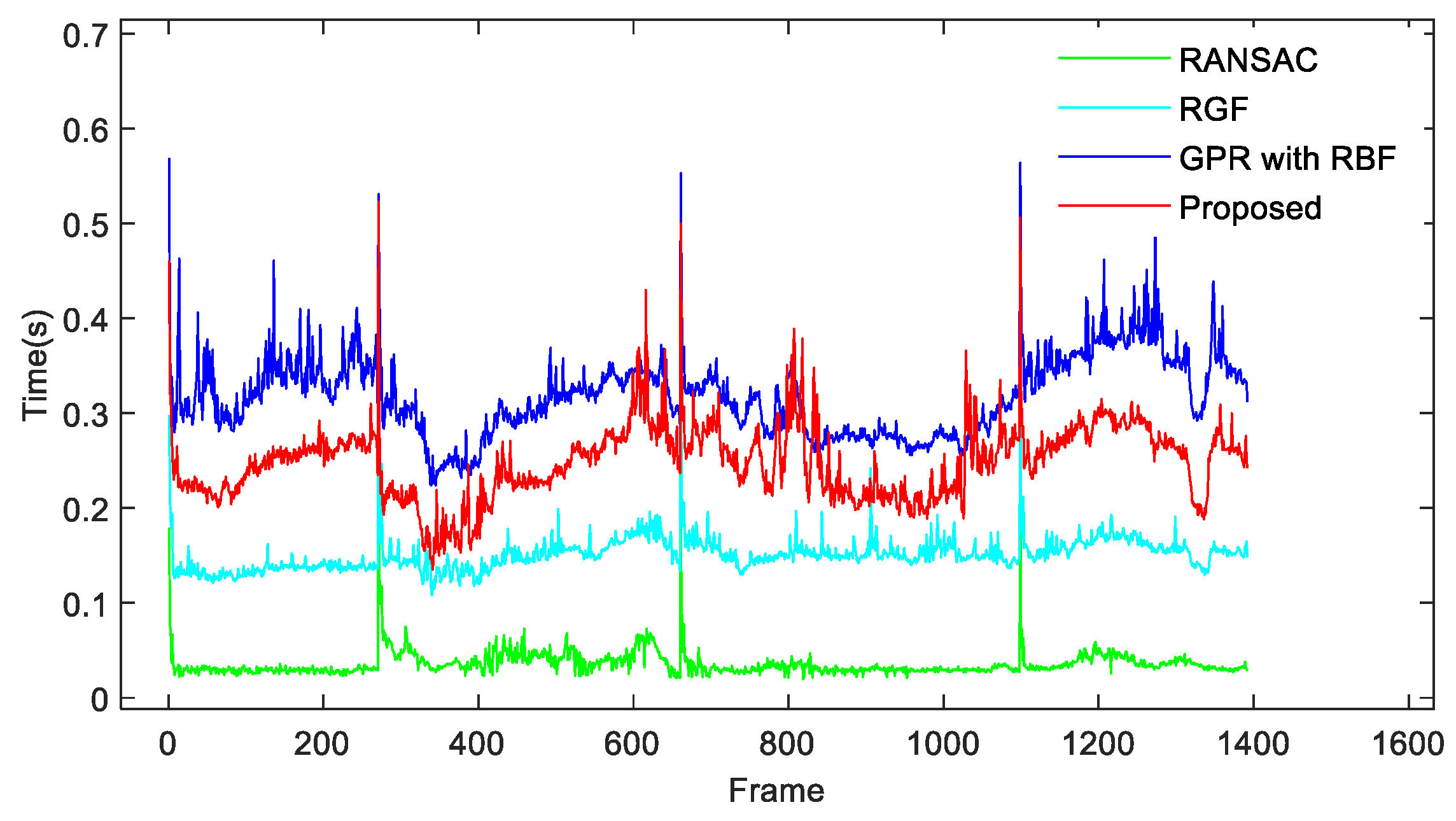
4. Experiments and Analysis
4.1. Hyperparameter Acquisition
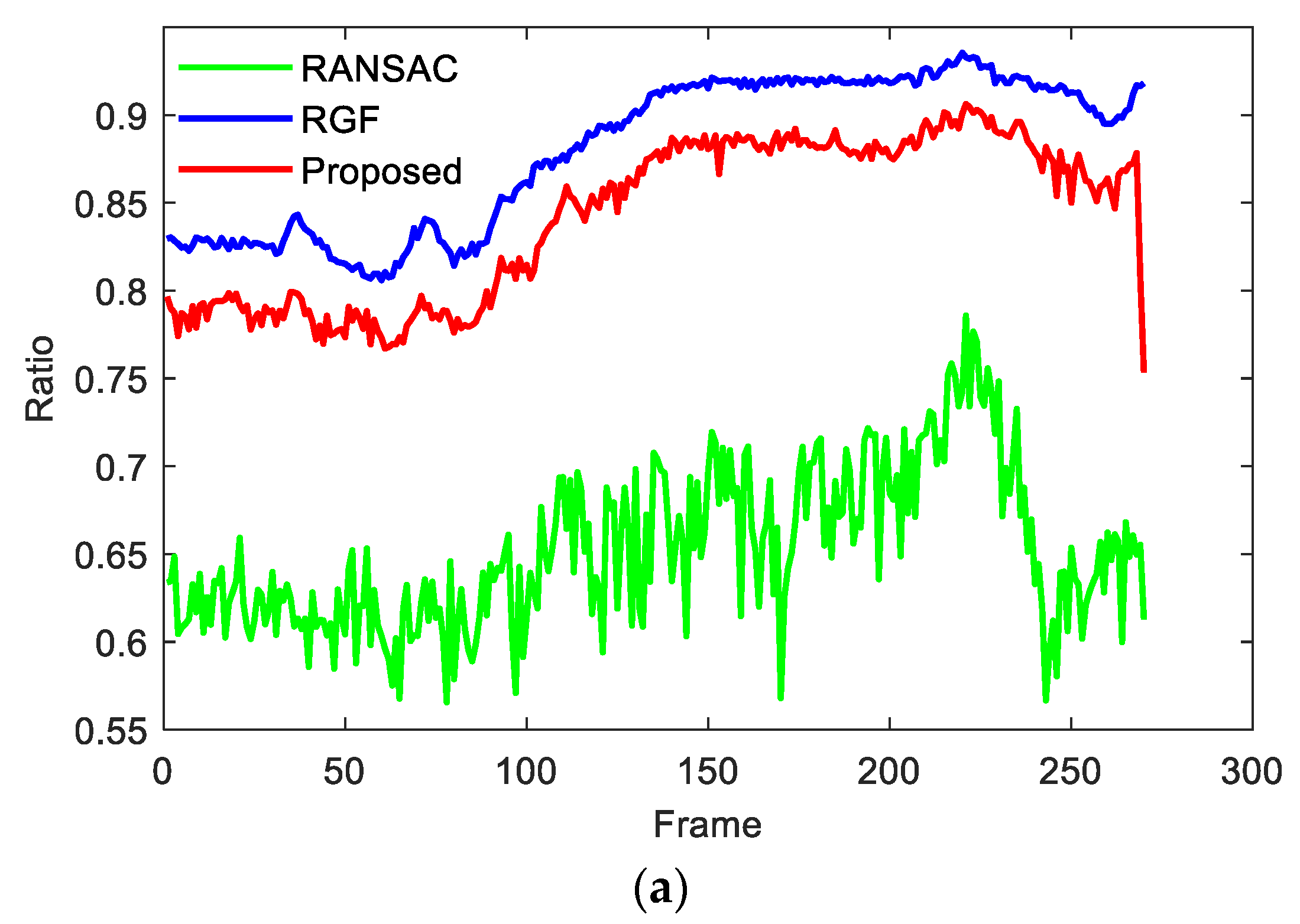
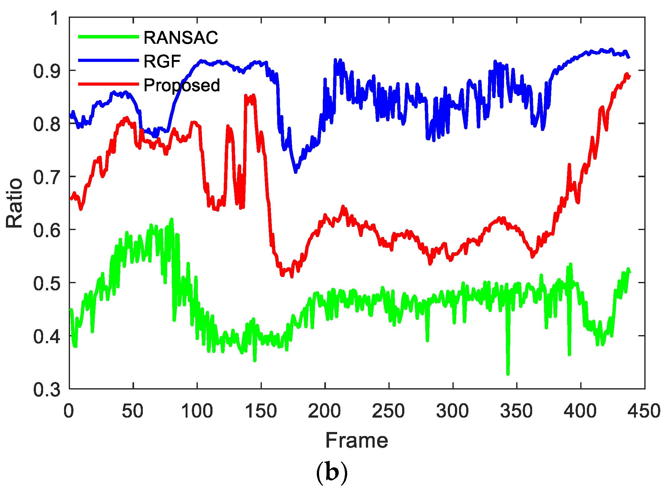
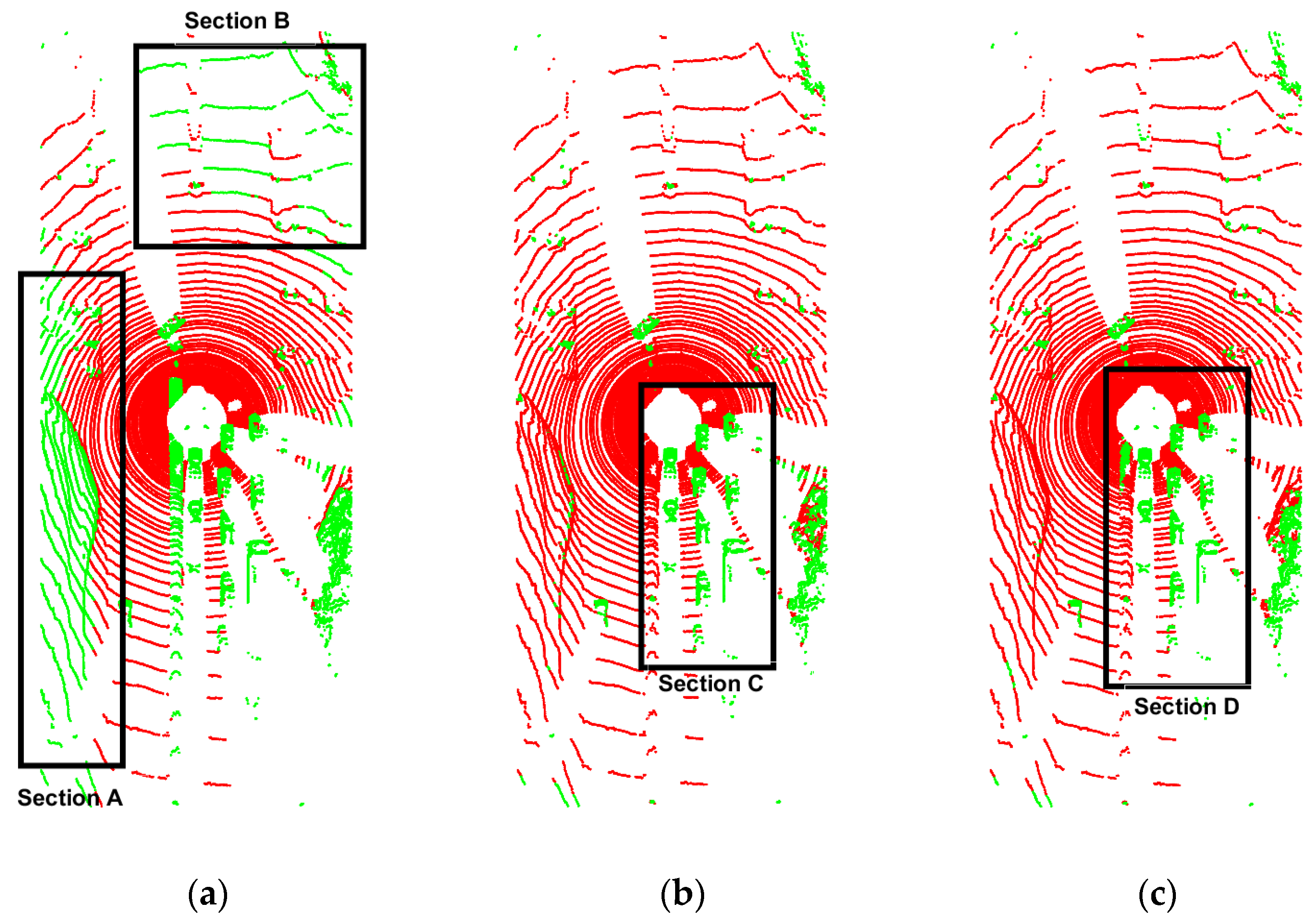
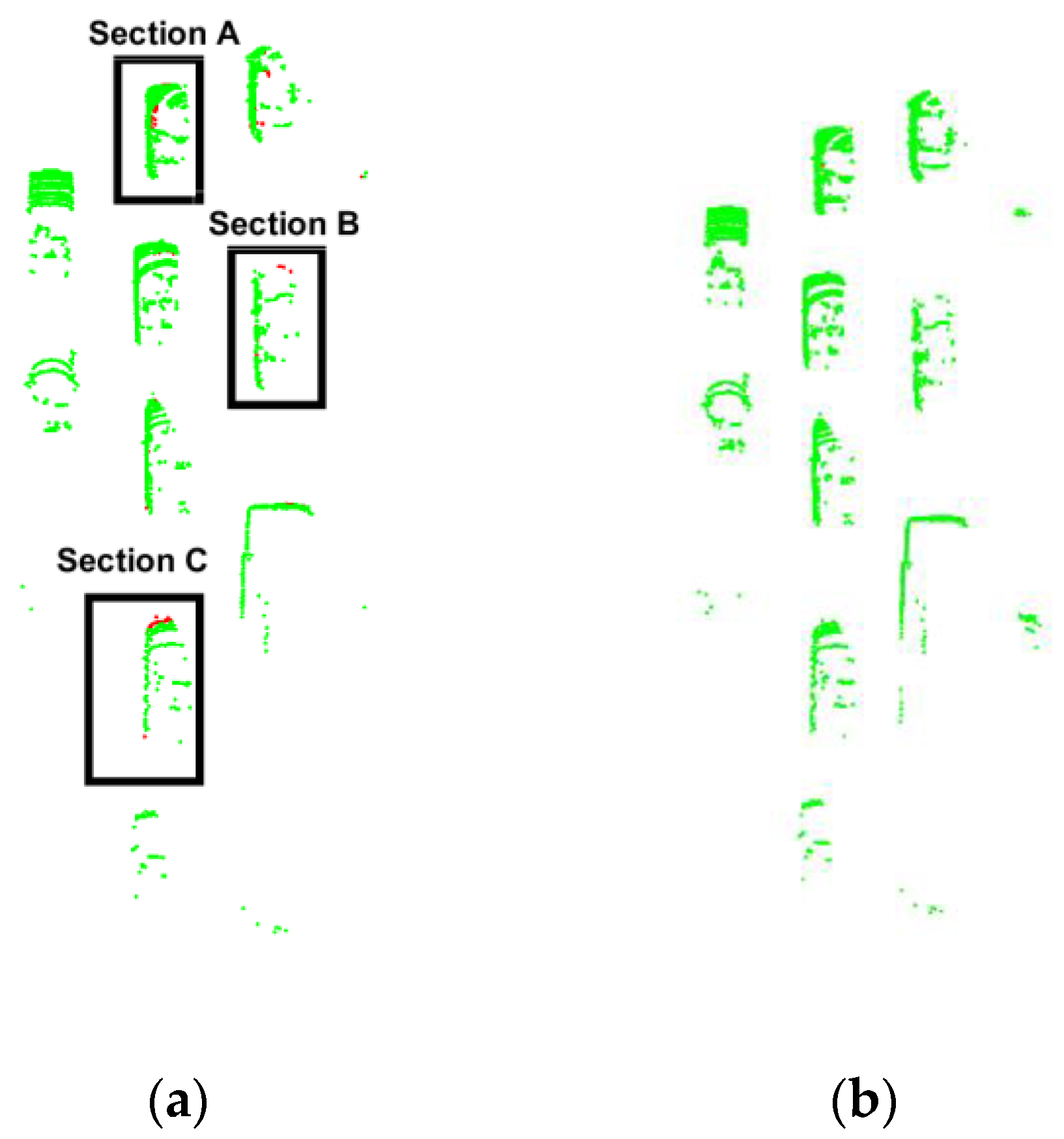
4.2. The Verification Effect of the Algorithm on the KITTI Dataset
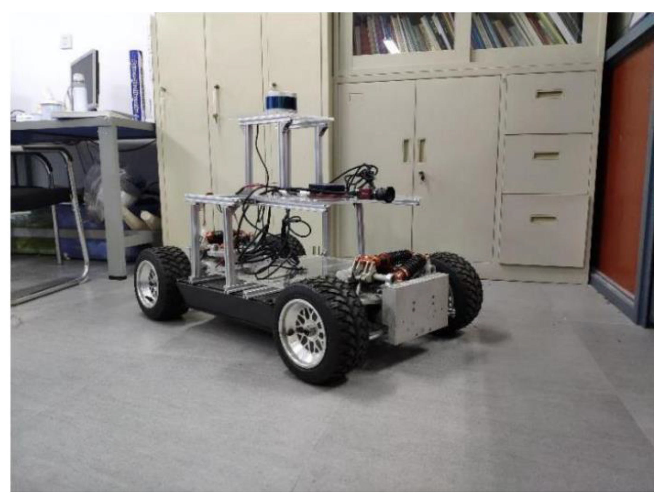
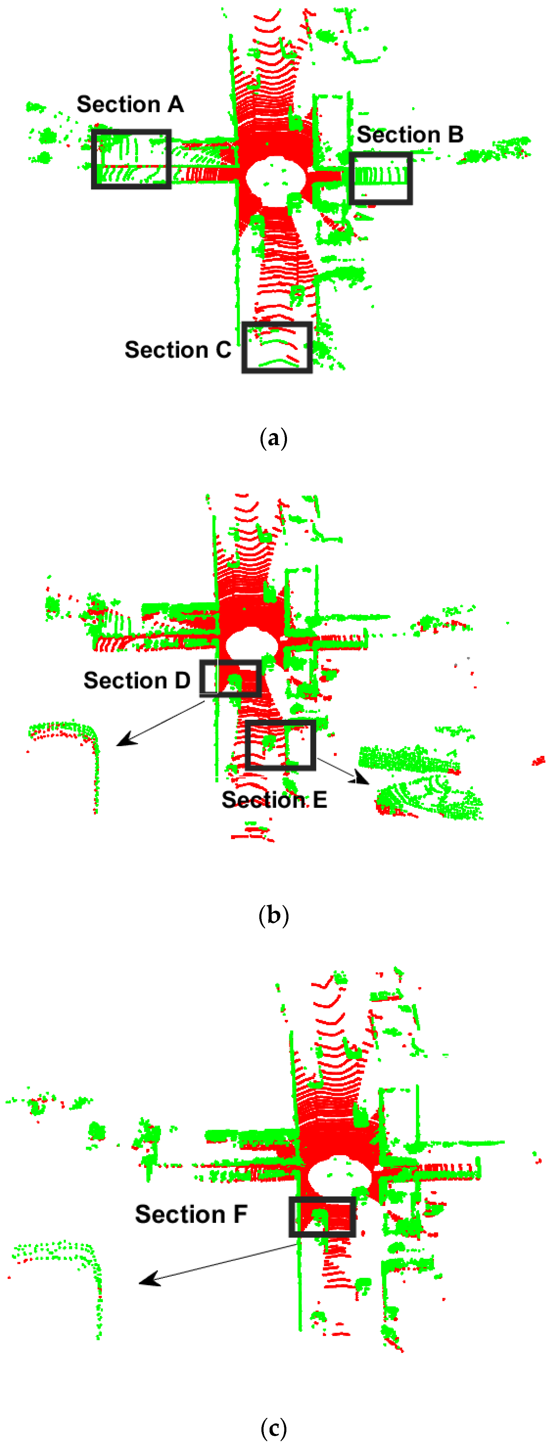
4.3. The verification Effect of the Algorithm on the Autonomous Driving Algorithm Verification Platform
5. Conclusions
Author Contributions
Funding
Institutional Review Board Statement
Informed Consent Statement
Data Availability Statement
Conflicts of Interest
References
- Li, Y.; Ma, L.; Zhong, Z.; Liu, F.; Chapman, M.A. Deep learning for lidar point clouds in autonomous driving: A review. IEEE Trans. Neural Netw. Learn. Syst. 2020, 32, 3412–3432. [Google Scholar] [CrossRef] [PubMed]
- Pendleton, S.D.; Andersen, H.; Du, X.; Shen, X. Perception, Planning, Control, and Coordination for Autonomous Vehicles. Machines 2017, 5, 6. [Google Scholar] [CrossRef]
- Mukhtar, A.; Xia, L.; Tang, T. Vehicle detection techniques for collision avoidance systems: A review. IEEE Trans. Intell. Transp. Syst. 2015, 16, 2318–2338. [Google Scholar] [CrossRef]
- Ye, Y.; Fu, L.; Li, B. Object detection and tracking using multi-layer laser for autonomous urban driving. In Proceedings of the 2016 IEEE International Conference on Intelligent Transportation Systems (ITSC), Riode Janeiro, Brazil, 1–4 November 2016. [Google Scholar]
- Wang, G.J.; Wu, J.; He, R.; Yang, S. A point cloud-based robust road curb detection and tracking method. IEEE Access 2019, 7, 24611–24625. [Google Scholar] [CrossRef]
- Jin, X.; Wang, J.; Yan, Z.; Xu, L.; Yin, G.; Chen, N. Robust Vibration Control for Active Suspension System of In-Wheel-Motor-Driven Electric Vehicle via μ-Synthesis Methodology. J. Dyn. Syst. Meas. Control 2022, 144, 051007. [Google Scholar] [CrossRef]
- Dai, Y.; Lee, S.G. Perception, planning and control for self-driving system based on on-board sensors. Adv. Mech. Eng. 2020, 12. [Google Scholar] [CrossRef]
- Dieterle, T.; Particke, F.; Patino-Studencki, L.; Thielecke, J. Sensor data fusion of LIDAR with stereo RGB-D camera for object tracking. In Proceedings of the 2017 IEEE Sensors, Glasgow, UK, 29 October–1 November 2017. [Google Scholar]
- Li, Y.; Ibanez-Guzman, J. Lidar for autonomous driving: The principles, challenges, and trends for automotive lidar and perception systems. IEEE Signal Process. Mag. 2020, 37, 50–61. [Google Scholar] [CrossRef]
- Zhao, C.; Fu, C.; Dolan, J.M.; Wang, J. L-Shape Fitting-based Vehicle Pose Estimation and Tracking Using 3D-LiDAR. IEEE Trans. Intell. Veh. 2021, 6, 787–789. [Google Scholar] [CrossRef]
- Sualeh, M.; Kim, G.W. Dynamic Multi-LiDAR Based Multiple Object Detection and Tracking. Sensors 2019, 19, 1474. [Google Scholar] [CrossRef] [PubMed] [Green Version]
- Kim, D.; Jo, K.; Lee, M.; Sunwoo, M. L-shape model switching-based precise motion tracking of moving vehicles using laser scanners. IEEE Trans. Intell. Transp. Syst. 2017, 19, 598–612. [Google Scholar] [CrossRef]
- Zhang, X.; Xu, W.; Dong, C.; Dolan, J.M. Efficient L-shape fitting for vehicle detection using laser scanners. In Proceedings of the 2017 IEEE Intelligent Vehicles Symposium (IV), Los Angeles, CA, USA, 11–14 June 2017. [Google Scholar]
- Jin, X.; Yang, H.; Li, Z. Vehicle Detection Framework Based on LiDAR for Autonoumous Driving. In Proceedings of the 2021 5th CAA International Conference on Vehicular Control and Intelligence (CVCI), Tianjin, China, 29–31 October 2021. [Google Scholar]
- Qiu, J.; Lai, J.; Li, Z.; Huang, K. A lidar ground segmentation algorithm for complex scenes. Chin. J. Sci. Instrum. 2020, 41, 244–251. [Google Scholar]
- Li, L.; Yang, F.; Zhu, H.; Li, D.; Li, Y.; Tang, L. An Improved RANSAC for 3D Point Cloud Plane Segmentation Based on Normal Distribution Transformation Cells. Remote Sens. 2017, 9, 433. [Google Scholar] [CrossRef] [Green Version]
- Douillard, B.; Underwood, J.; Kuntz, N.; Vlaskine, V.; Quadros, A.; Morton, P.; Frenkel, A. On the segmentation of 3D LIDAR point clouds. In Proceedings of the 2011 IEEE International Conference on Robotics and Automation, Shanghai, China, 9–13 May 2011. [Google Scholar]
- Rummelhard, L.; Paigwar, A.; Nègre, A.; Laugier, C. Ground estimation and point cloud segmentation using spatiotemporal conditional random field. In Proceedings of the 2017 IEEE Intelligent Vehicles Symposium (IV), Los Angeles, CA, USA, 11–14 June 2017. [Google Scholar]
- Himmelsbach, M.; Hundelshausen, F.V.; Wuensche, H.J. Fast segmentation of 3D point clouds for ground vehicles. In Proceedings of the 2010 IEEE Intelligent Vehicles Symposium, La Jolla, CA, USA, 21–24 June 2010. [Google Scholar]
- Chen, T.; Dai, B.; Wang, R.; Liu, D. Gaussian-Process-Based Real-Time Ground Segmentation for Autonomous Land Vehicles. J. Intell. Robot. Syst. Theory Appl. 2014, 76, 563–582. [Google Scholar] [CrossRef]
- Chen, T.; Dai, B.; Liu, D.; Song, J. Sparse Gaussian process regression based ground segmentation for autonomous land vehicles. In Proceedings of the 27th Chinese Control and Decision Conference (2015 CCDC), Qingdao, China, 23–25 May 2015. [Google Scholar]
- Luo, Z.; Mohrenschildt, M.; Habibi, S. A Probability Occupancy Grid Based Approach for Real-Time LiDAR Ground Segmentation. IEEE Trans. Intell. Transp. Syst. 2019, 21, 998–1010. [Google Scholar] [CrossRef]
- Narksri, P.; Takeuchi, E.; Ninomiya, Y.; Morales, Y.; Akai, N.; Kawaguchi, N. A slope-robust cascaded ground segmentation in 3D point cloud for autonomous vehicles. In Proceedings of the 2018 21st International Conference on Intelligent Transportation Systems (ITSC), Maui, HI, USA, 4–7 November 2018. [Google Scholar]
- Jiménez, V.; Godoy, J.; Artuñedo, A.; Villagra, J. Ground Segmentation Algorithm for Sloped Terrain and Sparse LiDAR Point Cloud. IEEE Access 2021, 9, 132914–132927. [Google Scholar] [CrossRef]
- Shen, Z.; Liang, H.; Lin, L.; Wang, Z.; Huang, W.; Yu, J. Fast Ground Segmentation for 3D LiDAR Point Cloud Based on Jump-Convolution-Process. Remote Sens. 2021, 13, 3239. [Google Scholar] [CrossRef]
- Chu, P.M.; Cho, S.; Park, J.; Fong, S.; Cho, K. Enhanced ground segmentation method for Lidar point clouds in human-centric autonomous robot systems. Hum.-Cent. Comput. Inf. Sci. 2019, 9, 17. [Google Scholar] [CrossRef] [Green Version]
- Zermas, D.; Izzat, I.; Papanikolopoulos, N. Fast segmentation of 3D point clouds: A paradigm on LiDAR data for autonomous vehicle applications. In Proceedings of the 2017 IEEE International Conference on Robotics and Automation (ICRA), Singapore, 29 May–3 June 2017. [Google Scholar]
- Zhang, Y.; Wang, J.; Wang, X.; Dolan, J.M. Road-segmentation-based curb detection method for self-driving via a 3D-LiDAR sensor. IEEE Trans. Intell. Transp. Syst. 2018, 19, 3981–3991. [Google Scholar] [CrossRef]
- Huang, W.; Liang, H.; Lin, L.; Wang, Z.; Wang, S.; Yu, B.; Niu, R. A Fast Point Cloud Ground Segmentation Approach Based on Coarse-To-Fine Markov Random Field. IEEE Trans. Intell. Transp. Syst. 2021, 1–14. [Google Scholar] [CrossRef]
- Melkumyan, A.; Ramos, F. A sparse covariance function for exact Gaussian process inference in large datasets. In Proceedings of the IJCAI International Joint Conference on Artificial Intelligence, Pasadena, CA, USA, 11–17 July 2009. [Google Scholar]


| Method | Ground Points | Non-Ground Points | Ratio of Ground Points |
|---|---|---|---|
| RANSAC | 23,316 | 13,219 | 63.82% |
| RGF | 30,306 | 6213 | 82.99% |
| Proposed | 29,396 | 7133 | 80.47% |
| Method | Ground Points | Non-Ground Points | Ratio of Ground Points |
|---|---|---|---|
| RANSAC | 15,844 | 37,869 | 29.56% |
| GPF | 20,545 | 31,064 | 39.91% |
| Proposed | 16,416 | 278,561 | 37.08% |
| Method | Ground Points | Non-Ground Points | Ratio of Ground Points |
|---|---|---|---|
| RANSAC | 9605 | 7187 | 57.2% |
| RGF | 10,168 | 6624 | 60.55% |
| Proposed | 10,665 | 6127 | 63.51% |
Publisher’s Note: MDPI stays neutral with regard to jurisdictional claims in published maps and institutional affiliations. |
© 2022 by the authors. Licensee MDPI, Basel, Switzerland. This article is an open access article distributed under the terms and conditions of the Creative Commons Attribution (CC BY) license (https://creativecommons.org/licenses/by/4.0/).
Share and Cite
Jin, X.; Yang, H.; Liao, X.; Yan, Z.; Wang, Q.; Li, Z.; Wang, Z. A Robust Gaussian Process-Based LiDAR Ground Segmentation Algorithm for Autonomous Driving. Machines 2022, 10, 507. https://doi.org/10.3390/machines10070507
Jin X, Yang H, Liao X, Yan Z, Wang Q, Li Z, Wang Z. A Robust Gaussian Process-Based LiDAR Ground Segmentation Algorithm for Autonomous Driving. Machines. 2022; 10(7):507. https://doi.org/10.3390/machines10070507
Chicago/Turabian StyleJin, Xianjian, Hang Yang, Xin Liao, Zeyuan Yan, Qikang Wang, Zhiwei Li, and Zhaoran Wang. 2022. "A Robust Gaussian Process-Based LiDAR Ground Segmentation Algorithm for Autonomous Driving" Machines 10, no. 7: 507. https://doi.org/10.3390/machines10070507