A Novel Decomposition-Based Multi-Objective Evolutionary Algorithm with Dual-Population and Adaptive Weight Strategy

Abstract

Multi-objective evolutionary algorithms mainly include the methods based on the Pareto dominance relationship and the methods based on decomposition. The method based on Pareto dominance relationship will produce a large number of non-dominated individuals with the increase in population size or the number of objectives, resulting in the degradation of algorithm performance. Although the method based on decomposition is not limited by the number of objectives, it does not perform well on the complex Pareto front due to the fixed setting of the weight vector. In this paper, we combined these two different approaches and proposed a Multi-Objective Evolutionary Algorithm based on Decomposition with Dual-Population and Adaptive Weight strategy (MOEA/D-DPAW). The weight vector adaptive adjustment strategy is used to periodically change the weight vector in the evolution process, and the information interaction between the two populations is used to enhance the neighborhood exploration mechanism and to improve the local search ability of the algorithm. The experimental results on 22 standard test problems such as ZDT, UF, and DTLZ show that the algorithm proposed in this paper has a better performance than the mainstream multi-objective evolutionary algorithms in recent years, in solving two-objective and three-objective optimization problems.

1. Introduction

In recent years, the field of multi-objective optimization has developed rapidly. A multi-objective optimization problem (MOP) refers to the existence of two or more conflicting objectives, the optimization of one which may lead to the deterioration of the other objectives, so that the globally unique optimal solution cannot be obtained, as in a single objective optimization problem. Multi-Objective Evolutionary Algorithm (MOEA) is often used to solve this kind of problem, which is usually based on the continuous iterative evolution of individuals in the population, and it finally obtains the solution set with uniform distribution and good convergence.

The current mainstream MOEAs can be divided into three categories, respectively: the method based on the Pareto dominance relationship, the method based on evaluation metrics, and the method based on decomposition. The basic idea of MOEAs, based on Pareto dominance relationship is to generate the next generation population according to certain hybridization and mutation strategies, order all individuals in the population according to the dominance relationship, and screen individuals according to the degree of individual dominance and the sparsity of the objective space. Deb et al. [1] improved the classical NSGA algorithm, introduced the concept of congestion degree, proposed the elite selection strategy, and designed the fast non-dominated sorting algorithm, NSGA-II, with the elite selection strategy. On the basis of this algorithm framework, they also proposed a multi-objective evolutionary algorithm, NSGA-III [2], based on reference points, which pays more attention to the non-dominant individuals in the population, and achieves a good performance in solving high-dimensional MOPs. Yuan et al. [3] improved the NSGA-II algorithm for job-shop scheduling problems in an intelligent manufacturing environment, adopted a process-based random mutation strategy and a crossover method to generate a new generation of population, and adopted the analytic hierarchy process to determine the optimal solution. Zhang et al. [4] introduced the rotation characteristic into the simulated binary crossover operator SBX and proposed an improved simulated binary crossover algorithm RSBX based on rotation and the combination with NSGA-II to significantly improve the performance of the algorithm. Yi et al. [5] introduced an adaptive mutation operator to improve the standard NSGA-III algorithm and to enhance the ability of the algorithm to solve complex optimization problems. Based on the NSGA-III algorithm, Cui et al. [6] used the selection operator to determine the reference point of the minimum ecological digit, and then selected an individual with the shortest boundary intersection distance, based on punishment, to better balance convergence and diversity. Gu et al. [7] introduced the information feedback model and proposed an improved algorithm, IFM-NSGA-III, which used the historical information of individuals in previous generations in the updating process of the current generation.

The method is based on evaluation metrics such as Inverted Generational Distance (IGD) and Hypervolume (HV), which are used to guide the population closer to the Pareto front. Sun et al. [8] proposed a method based on IGD metrics in order to select excellent individuals in each generation of individuals, and designed an efficient dominant comparison method to rank the results. Hong et al. [9] developed a new metrics-based algorithm that uses an enhanced diversification mechanism, combined a new solution generator and an external archive, and used a double local search mechanism to search different subregions of the Pareto front. Yuan et al. [10] introduced a cost-value-based distance into the target space to evaluate the contributions of individuals to explore potential fields, proposed a metrics-based CHT algorithm and embedded it into the evolutionary algorithm, achieving good experimental results in the MOPs where individuals appear in the local infeasible region. Li et al. [11] proposed a multi-modal MOEA based on weighted indexes, named MMEA-WI, and integrated the diversity information of solutions in the decision space into a performance index of target space to ensure that the Pareto front can be approached more effectively. Li et al. [12] believed that the evaluation of evolutionary algorithms is essentially a binary classification, and then proposed an online asynchronous training method of a support vector machine model based on empirical kernel, to classify promising and unpromising solutions, and then reversely added the newly generated solutions as training samples to improve the accuracy of the classifier. Garcia et al. [13] proposed an metrics-based algorithm COARSE-EMOA to solve the MOPs with equality constraints. A reference set of a feasible Pareto front was used to calculate the generation distance, and then it was used as the density estimation to obtain a better solution set distributed near the Pareto front.

Zhang et al. [14] proposed a Multi-Objective Evolutionary Algorithm based on Decomposition (MOEA/D), which provided a new idea for MOEAs. This kind of algorithm no longer uses the traditional Pareto dominance relationship to guide the population evolution, but it uses the aggregation function to decompose the multi-objective problem into a number of simple single-objective problems, and co-evolve. The weight vector is used to control the direction of population evolution, which greatly reduces the computational complexity of the algorithm and has strong searching ability. It has become a classic method to solve MOPs, and has been continuously improved and extended by scholars, based on this algorithm. Zhu et al. [15] proposed a decomposed multi-objective evolutionary algorithm MOEA/D-DAE based on detection escape strategy in order to solve the problem that the algorithm is prone to stagnation in the complex feasible domain of constrained multi-objective optimization problems. Cao et al. [16] used the multi-population heuristic algorithm PBO as an effective search engine, and proposed a new multi-objective evolutionary algorithm MOEA/D-PBO based on decomposition. Wang et al. [17] proposed an improved algorithm AES-MOEA/D based on an adaptive evolutionary strategy, and adopted the evolutionary strategy of competition between the SBX and DE operators to overcome the problem of species diversity degradation caused by a single operator. Xie et al. [18] designed an improved algorithm, DTR-MOEA/D, with local target space knowledge and the dynamic transfer of reference points, established the dynamic transfer criterion of reference points according to the population density relationship in different regions, and adopted the population diversity enhancement strategy guided by regional target space knowledge to improve the population diversity. Chen et al. [19] used the improved directions in the current and historical populations to generate new solutions, and introduced this mechanism into the MOEA/D-PBI algorithm, greatly improving the convergence ability of the algorithm.

In solving practical problems, Zhang et al. [20] designed a novel integral squeeze film bearing damper based on the multi-objective optimization problem, and combined the non-dominated sorting genetic algorithm and grey correlation analysis for the multi-objective optimization of stiffness and stress. Akbari et al. [21] designed and optimized the blades of small wind turbines to maximize power output and starting torque. They took the chord length and the twist angle as design variables, and used a multi-objective optimization study to evaluate the optimal blade geometry. Jiang et al. [22] proposed a multi-objective optimization procedure combined with the NSGA-II algorithm with entropy weighted TOPSIS for the lightweight design of a dump truck carriage, and the multi-objective lightweight optimization of the dump truck carriage was carried out based on the Kriging surrogate model and the NSGA-II algorithm.

On the basis of referring to plenty of relevant work and experimental analysis, this paper makes a comprehensive comparison and analysis of two major methods, respectively: MOEAs based on Pareto dominance relationship and MOEAs based on decomposition. MOEAs based on Pareto dominance relationship usually use a non-dominated sorting algorithm to sort population individuals and to introduce a crowding degree operator to filter out overlapping individuals in the population, which can better maintain the diversity of population individuals, but there is also an obvious problem, where in the face of MOPs with a complex Pareto front, the searching ability of the algorithm is poor, and the convergence rate of the individual population is slow. However, MOEAs based on decomposition are different. Since the decomposition method is used to transform multi-objective optimization problems into multiple single-objective optimization problems, the individual searching ability of such methods is strong, and it is easier to search the boundary of Pareto front, but the problem of an uneven searching ability is likely to occur when facing complex MOPs. Therefore, it is very necessary to combine these two types of mainstream algorithms and to put forward a more comprehensive method which can avoid the defects of these two types of algorithms. At the same time, some new mechanisms and strategies should be introduced to ensure the smooth progress of the search process. Based on the above analysis, the research roadmap of the algorithm proposed in this paper is formed, as shown in Figure 1.

In this paper, we combined MOEAs based on Pareto dominance relationship and MOEAs based on decomposition, and proposed an improved algorithm called MOEA/D, with Dual-Population and Adaptive Weight strategy (MOEA/D-DPAW). In the process of iterative evolution, two different populations are set up to complete the evolution in their own way. The two groups exchange and share information with each other, resulting in better individuals. Furthermore, MOEA/D-DPAW used the Pareto dominance relationship between individuals and the crowding degree operator to ensure the diversity of the population, and used the weight vector adaptive adjustment strategy and enhanced neighborhood search mechanism to improve the local search ability of the algorithm in complex space to ensure the convergence of the algorithm. The final solution set obtained by the algorithm can maintain a more uniform distribution of a population of individuals on the premise of approximately fitting the real Pareto front.

The remainder of the paper is organized as follows. Section 2 introduces the previous knowledge. In the Section 3, the proposed algorithm framework and related improvement strategies are described in detail. Section 4 is the experimental part which compares and analyzes the proposed algorithm with the mainstream evolutionary multi-objective optimization algorithm in recent years. Section 5 summarizes the main work of this paper and points out further research directions.

2. Previous Knowledge

2.1. Problem Model

Taking minimization MOP as an example, it can be formulated as follows:

$$\begin{array}{c}\hfill minimizeF\left(x\right)={(f_1\left(x\right),f_2\left(x\right),\dots ,f_m\left(x\right))}^T\hfill \\ \hfill subjecttox\in X\hfill \end{array}$$

(1)

where $x={(x_1,x_2,\dots ,x_n)}^T\in X$ is an n-dimensional decision vector in space $R^n$, and X represents the decision space formed by all decision variables. $y=(f_1\left(x\right),f_2\left(x\right),\dots ,f_m\left(x\right))\in Y$ is an m-dimensional optimization objective, and Y represents the objective space formed by all optimization objectives. m is the number of optimization objectives. For a viable solution $x^{*}\in X$, if and only if there is no other viable solution $x\in X$ satisfying $f_i\left(x\right)\le f_i\left(x^{*}\right),i=1,2,\dots ,m$, and there is at least one $j\in \{1,2,\dots ,m\}$ that makes $f_j\left(x\right)\le f_j\left(x^{*}\right)$ valid, then x is called a Pareto optimal solution of the MOP. In the decision space, all feasible solutions satisfying the Pareto optimal solution conditions form the Pareto optimal solution set $PS\subseteq X$. In the corresponding objective space, the definition of Pareto front is $PF=\left\{F\right(x\left)\right|x\in PS\}$. The essence of MOPs is to make the individuals in the population approach the real Pareto front, and to finally find a group of compromise solutions approaching the Pareto front.

2.2. Dominance Relationship and Crowding Degree

For MOPs, it is assumed that individuals p and q are two solutions in the population. If p is better than q, then p dominates q. Specifically, two conditions must be satisfied: (1) For all targets, individual p is no worse than q; that is, $f_i\left(p\right)\le f_i\left(q\right),i=1,2,\dots ,m$. (2) There is at least one objective for which p is better than q, that is, $\exists i\in \{1,2,\dots ,m\}$ satisfies $f_i\left(p\right)<f_i\left(q\right)$. In the process of population evolution, there will be many non-dominated individuals. When the population size exceeds the capacity initially set, it is necessary to use the fast non-dominated sorting algorithm to select individuals with high convergence as much as possible, and to maintain the diversity of the population through the crowding degree operator. In this paper, the crowding degree of individual p in population P is defined as follows:

$$\begin{array}{c}\hfill Crowding\left(p\right)=1-\prod _{q\in P,q\ne p}f(p,q)\end{array}$$

(2)

$$f(p,q)=\left\{\begin{array}{cc}\hfill \frac{distance(p,q)}{R},\hfill & \hfill distance(p,q)\le R\\ \hfill 1,\hfill & \hfill otherwise\end{array}\right.$$

(3)

where $Crowding\left(p\right)$ represents the crowding degree of individual p, and $distance(p,q)$ represents the Euclidean distance between individuals p and q in the decision space. R is the size of the neighborhood radius. According to the Equations (2) and (3), the crowding degree of individuals is always within the range of [0,1]. The crowding degree of an individual in a population depends on the number and distance of other individuals in its neighborhood. The greater the number of individuals in the neighborhood, or the smaller the Euclidean distance between an individual in the neighborhood and the current individual, the greater the crowding degree of the individual will be, and the easier it will be to be eliminated during population maintenance. In the process of the population maintenance operation, the most crowded individuals are constantly removed. If there are multiple individuals with the most crowded degree, one of them will be randomly selected, and then the crowding degree of other individuals belonging to the removed individual neighborhood will be updated. This process is repeated until the population size is satisfied.

2.3. Method of Decomposition

In the MOEA/D algorithm and its variants, the core idea is to split the multi-objective optimization problem into a set of scalar optimization problems, and to optimize a set of scalar optimization problems simultaneously. Each subproblem only needs to combine the information provided by several neighboring subproblems to complete the optimization calculation. First, a set of weight vectors $\lambda ={({\lambda }_1,{\lambda }_2,\dots ,{\lambda }_m)}^T,{\lambda }_i\ge 0$ should be initialized to meet the condition ${\sum }_{i=1}^m{\lambda }_i=1$. There are three common decomposition methods for all decision variables x in the decision space $x\in X$, as follows:

• Weighted Sum approach: The weight vector is used as a coefficient corresponding to the objective function one by one, and the mathematical formula is shown as below:

  $$\begin{array}{c}\hfill minimize{g}^{ws}\left(x\right|\lambda )=\sum _{i=1}^m{\lambda }_i{f}_i\left(x\right)\end{array}$$

  (4)

  where $g^{ws}$ is the aggregate function that needs to be minimized. The idea of the decomposition method is simple, and it is only applicable to the regular Pareto front, and the effect is poor when dealing with problems with a complex Pareto front.
• Tchebycheff approach: The decomposition method formula of this method is shown as below:

  $$\begin{array}{c}\hfill minimize{g}^{te}\left(x\right|\lambda ,z^{*})=ma{x}_{1\le i\le m}\{{\lambda }_i|f_i\left(x\right)-z_i^{*}\left|\right\}\end{array}$$

  (5)

  where $g^{te}$ is the aggregate function that needs to be minimized, and $z^{*}={(z_1^{*},z_2^{*},\dots ,z_m^{*})}^T$ is a set of reference points satisfying $z_i^{*}\le min\left\{f_i\left(x\right)\right|x\in X\}$. For any Pareto optimal solution x, there will be a set of weight vector $\lambda$ which makes x become the optimal solution in the Tchebycheff equation. This method can be used to obtain different Pareto optimal solutions by changing the weight vector. Because this method has a good effect on most problems, has universality, and is easy to implement, so in the experimental part, this paper chooses the Tchebycheff decomposition method.
• Penalty-based Boundary Intersection approach: This method attempts to find the intersection point between a group of rays passing through the target space from an ideal point and the Pareto front. If these rays are uniformly distributed, then the intersection points found will be approximately uniformly distributed:

  $$\begin{array}{c}\hfill minimize{g}^{pbi}\left(x\right|\lambda ,z^{*})=d_1+\theta d_2\end{array}$$

  (6)

  $$\begin{array}{c}\hfill d_1=\frac{∥\begin{array}{c}{(z^{*}-F\left(x\right))}^T\lambda \end{array}∥}{∥\begin{array}{c}\lambda \end{array}∥}\end{array}$$

  (7)

  $$\begin{array}{c}\hfill d_2=\Vert F\left(x\right)-(z^{*}-d_1\frac{\lambda }{∥\begin{array}{c}\lambda \end{array}∥})\Vert \end{array}$$

  (8)

  where $g^{pbi}$ is the aggregate function that needs to be minimized, $\theta$ is the penalty parameter, and the meaning of $z^{*}$ is the same as the Tchebycheff approach. Let y be the projection point of $F\left(x\right)$ on the ray, with $z^{*}$ as the origin and $-\lambda$ as the direction vector, then $d_1$ is the distance between y and $z^{*}$, and $d_2$ is the distance between y and $F\left(x\right)$. When using this method, the penalty parameter $\theta$ is very important, and the setting of $\theta$ will directly determine the final performance of the algorithm. However, when solving practical problems, it is difficult to determine the size of parameter $\theta$ at the beginning, and so this method is not used in the experimental part of this paper.

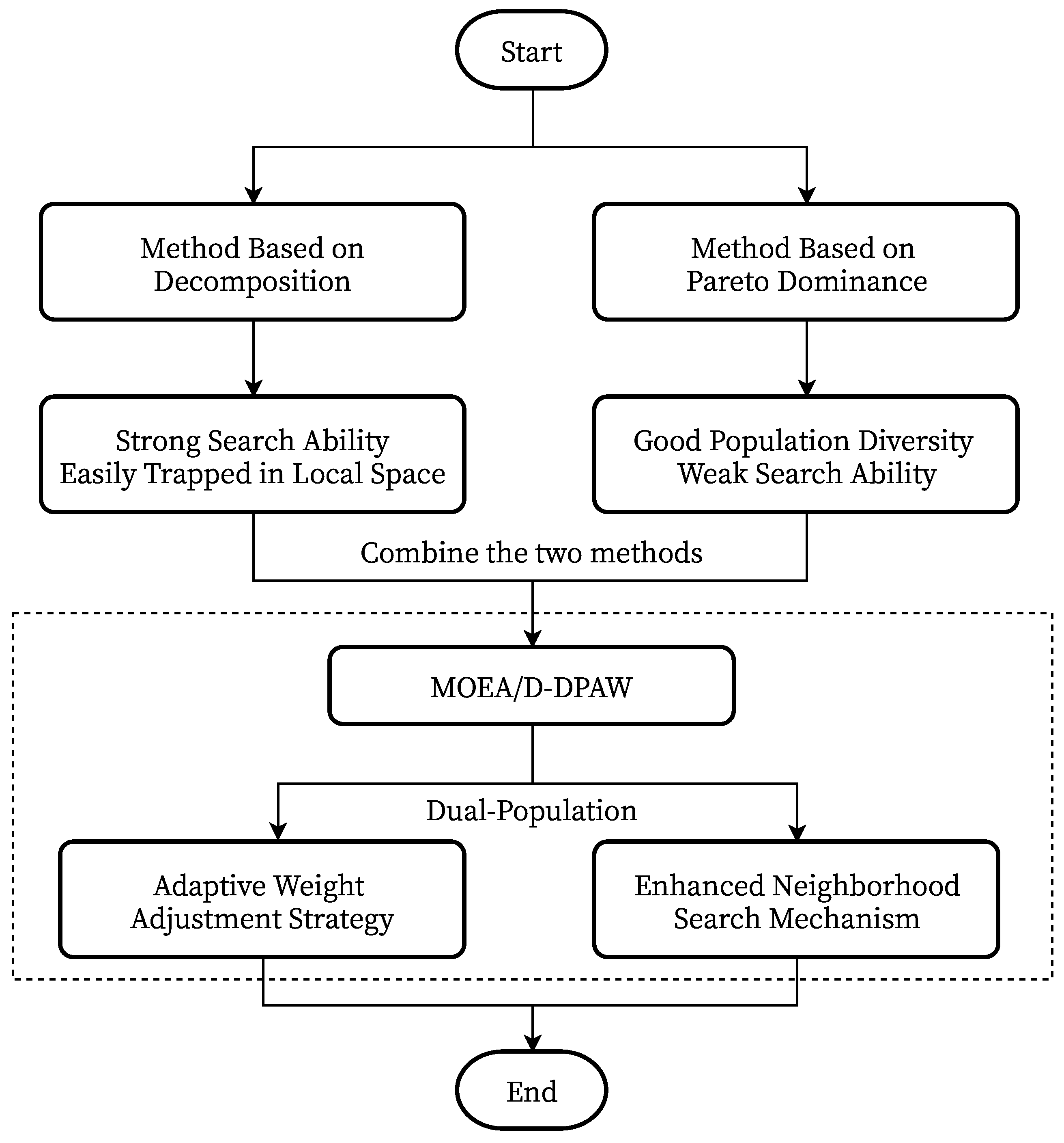
3. Proposed Algorithm

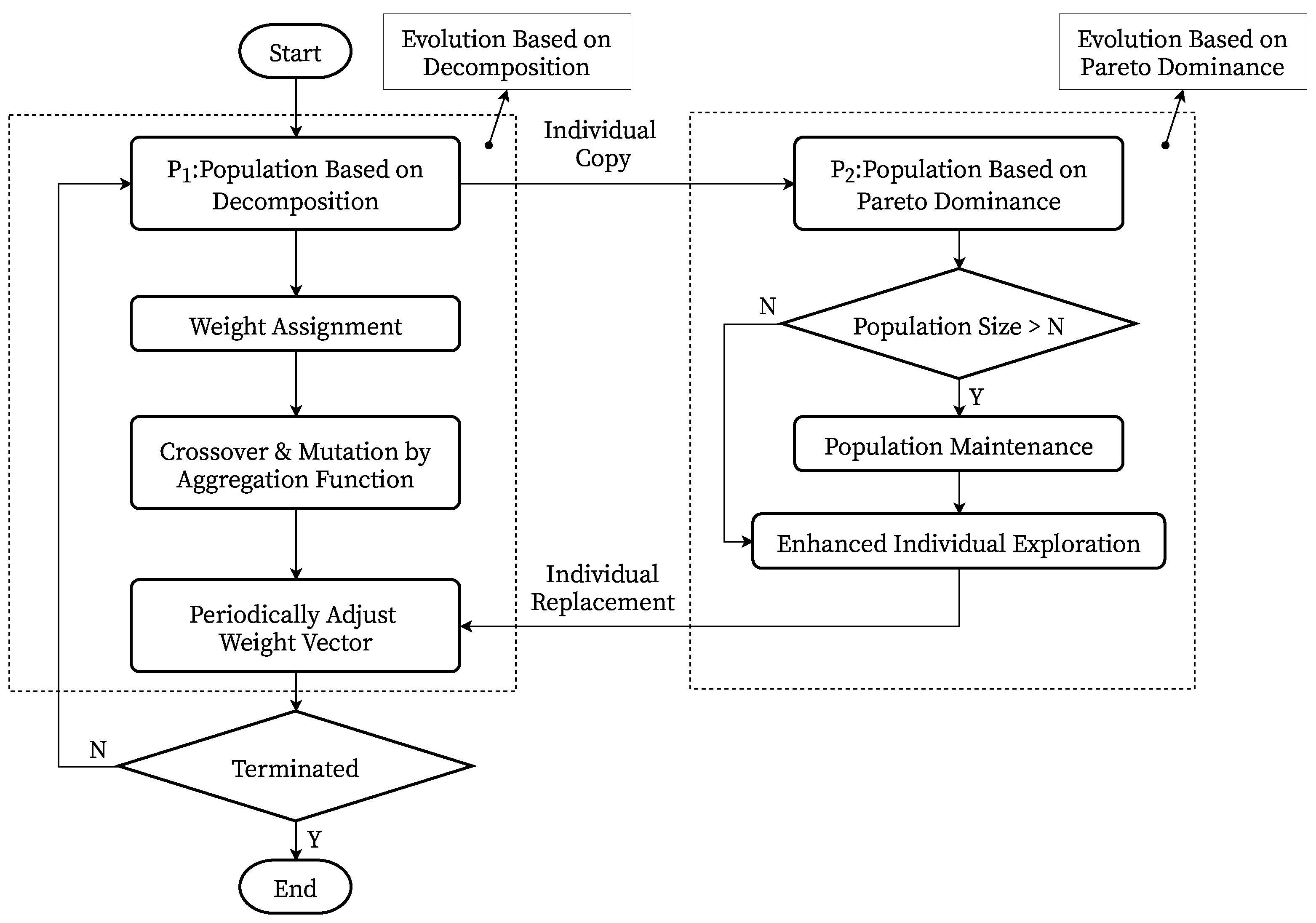
3.1. Framework

In this paper, we proposed a Multi-Objective Evolutionary Algorithm Based on Decomposition with Dual-Population and Adaptive Weight strategy (MOEA/D-DPAW). The framework of the algorithm is shown in Figure 2. There are two different populations in MOEA/D-DPAW, which are respectively used in the evolutionary algorithm based on decomposition and the evolutionary algorithm based on Pareto domination. During each iteration, two populations evolve in their own way, exchanging and sharing information with each other, resulting in better individuals.

In order to ensure the convergence of the algorithm, the evolutionary population $P_1$ will continue to evolve according to the MOEA/D based on the Tchebycheff decomposition approach. Firstly, the corresponding weight vector will be assigned to all individuals, and then the genetic operator will be used for each subproblem to generate new solutions in its neighborhood. After that, the update operation of the population individuals and ideal points will be completed. An external population $EP$ is maintained in the process, to collect all the non-dominant solutions during the evolution of the population. In addition, because the evenly distributed fixed weight vector is not conducive to solving the complex MOPs, in the process of population $P_1$ evolution, MOEA/D-DPAW uses the weight vector adaptive adjustment strategy to periodically adjust the weight vector, which makes the algorithm more applicable to practical problems, and makes the population of individuals closer to the Pareto front. This is covered in more detail in Section 3.2. At the same time, due to the limitation of neighborhood, the individual exploration of population $P_1$ will always focus on some specific areas in the objective space, so the algorithm has a poor search ability when facing a complex Pareto front. To solve this problem, MOEA/D-DPAW uses the enhanced neighborhood exploration mechanism. By means of further interaction between the individuals in population $P_2$ and population $P_1$, the exploration range of individuals in population $P_1$ is expanded, thus further improving the search ability of the algorithm. This part will be introduced in detail in Section 3.3.

In terms of maintaining the individual diversity of the population, MOEAs based on decomposition often lack some specific methods to avoid the problem of uneven distribution of individuals within the population. In the face of complex MOPs, the individuals of the population may be concentrated in some specific areas. In view of this, the evolutionary population $P_2$ based on the Pareto dominance relationship is introduced into the MOEA/D-DPAW algorithm. Before each iteration evolution, population $P_2$ will merge with individuals in population $P_1$, and then it conducts a fast non-dominated sorting of the resulting population. Based on the concept of crowding degree that is proposed in Section 2.2, population maintenance operations will be carried out. On the premise of ensuring the uniform distribution of individuals, excellent individuals will be selected for the subsequent enhanced neighborhood exploration mechanism. To sum up, the overall algorithm of MOEA/D-DPAW is shown in Algorithm 1. Lines 7 to 13 are the evolutionary process, based on the Pareto dominance relationship. Lines 14 to 33 are the evolutionary process based on decomposition; specifically, lines 19 to 23 are the process of updating the subproblem using the Tchebycheff formula, and lines 24 to 31 are the process of maintaining the external population EP. Finally, lines 34 to 36 are the call of the weight vector adaptive adjustment strategy, and line 37 is the call of the enhanced neighborhood exploration mechanism, which can refer to the contents of Section 3.2 and Section 3.3, respectively.

Algorithm 1 MOEA/D-DPAW

1: $EP\leftarrow ⌀$   2: Initialize the population $P_1,P_2$ and the weight vector set $\lambda$   3: Determine the neighbors $B_i$ from each weight vector of ${\lambda }_i$   4: Calculate the reference point $z^{*}$ according to $P_1$   5: $Gen\leftarrow 0$   6: while $Gen\le Ge{n}_{Max}$  do   7:    $P_2\leftarrow P_1\cup P_2$   8:    Fast-non-dominated-sort($P_2$) and calculate crowding degree C by Equations (2) and (3)   9:    while |$P_2$|>N do 10:       Randomly select the individual p which has highest crowding degree 11:       $P_2\leftarrow P_2\setminus p$ 12:       Update C about the neighbors of p 13:     end while 14:     $O\leftarrow ⌀$ 15:     for all $i\in \{1,2\dots N\}$ do 16:      Randomly select mating solutions from $B_i$ to generate an offspring $\overline{x}$ 17:     $z^{*}\leftarrow min(z^{*},F\left(\overline{x}\right))$ 18:     $O\leftarrow O\cup \overline{x}$ 19:     for all $j\in B_i$ do 20:        if $g^{te}\left(\overline{x}\right|{\lambda }_j,z^{*})\le g^{te}\left(x_j\right|{\lambda }_j,z^{*})$ then 21:           $x_j\leftarrow \overline{x}$ 22:        end if 23:     end for 24:     for all $o\in O$ do 25:        if $\nexists q\prec EP,q<o$ then 26:          $EP\leftarrow EP\cup o$ 27:          $EP\leftarrow EP\setminus \{q\in EP|o\prec q\}$ 28:        end if 29:        while |$EP$|>$2N$ do 30:          Remove the individual with the highest crowding distance from $EP$ 31:        end while 32:      end for 33:    end for 34:     if $Gen$ % (5% × $Ge{n}_{Max}$)=0 then 35:       Adaptive-Weight-Strategy($P_1,\lambda ,EP,N$) by Algorithm 2 36:     end if 37:     Enhanced-Individual-Exploration($P_1,P_2$) by Algorithm 3 38: end while 39: return  $P_1$

3.2. Adaptive Weight Strategy

It can be seen from the three decomposition methods in Section 2.3 that the setting of the size of the weight vector is crucial. Each different weight vector corresponds to a unique sub-problem that is formed after decomposition. However, in the original MOEA/D algorithm, the weight vector is fixed at the initialization, and there will be no changes afterwards, so that it is difficult to immediately determine the most appropriate weight vector size in the face of complex MOPs. To solve this problem, the MOEA/D-DPAW algorithm proposed in this paper uses the weight vector adaptive adjustment strategy, and periodically adjusts the weight vector in the process of population evolution, which can make these decomposed subproblems approach to the real Pareto front better. In the initialization phase, MOEA/D-DPAW uses a uniform random method to generate an initial set of weight vectors $\lambda ={({\lambda }_1,{\lambda }_2,\dots ,{\lambda }_m)}^T\in R^m$. WS-transform [23] is applied to project the weight vector of the scalar quantum problem to its solution mapping vector:

$$\begin{array}{c}\hfill \lambda =WS\left(\lambda \right)=(\frac{\frac{1}{{\lambda }_1}}{{\sum }_{i=1}^m\frac{1}{{\lambda }_i}},\frac{\frac{1}{{\lambda }_2}}{{\sum }_{i=1}^m\frac{1}{{\lambda }_i}}\dots \frac{\frac{1}{{\lambda }_m}}{{\sum }_{i=1}^m\frac{1}{{\lambda }_i}})\end{array}$$

(9)

In the process of population evolution, MOEA/D-DPAW will periodically adjust the weight vector every 5%T interval, where T is the number of evolution generation. During the weight vector adjustment, Equation (10) was used to calculate individual sparsity first for the individual p, and then the most crowded 5%N subproblems were removed, where N is the population size.

$$\begin{array}{c}\hfill Sparsity\left(p\right)=\prod _{i=1}^{m}distance(p,q_i)\end{array}$$

(10)

MOEA/D-DPAW uses the external population $EP$ to store the non-dominated solutions found during the search. When adjusting the weight vector to create a new subproblem, Equation (10) should be used to calculate the sparse degree of individuals in $EP$ relative to the current population. Then, the sparsest individual $x^s$ in $EP$ should be selected each time to generate a new subproblem and to calculate its objective function value $F\left(x^s\right)=(f_1^s,f_2^s,\dots ,f_m^s)$. Finally, Equation (11) should be used to generate a new weight vector $\lambda$ and associate with it, and this new subproblem is added to the population. The specific process of the Adaptive Weight Strategy algorithm is shown in Algorithm 2.

$$\begin{array}{c}\hfill {\lambda }^s=(\frac{\frac{1}{f_1^s-z_1^{*}}}{{\sum }_{i=1}^m\frac{1}{f_i^s-z_i^{*}}},\frac{\frac{1}{f_2^s-z_2^{*}}}{{\sum }_{i=1}^m\frac{1}{f_i^s-z_i^{*}}}\dots \frac{\frac{1}{f_m^s-z_m^{*}}}{{\sum }_{i=1}^m\frac{1}{f_i^s-z_i^{*}}})\end{array}$$

(11)

Algorithm 2 Adaptive Weight Strategy

Require:  P (Population), $\lambda$ (Weight vectors), $EP$ (External population), N (Population size)   1: $\theta \leftarrow 0.05N$   2: $count\leftarrow 0$   3: while  $count<\theta$  do   4:    Calculate the sparsity degree of each individual using Equation (2) and (3)   5:    Remove the individual with the minimum sparsity degree   6:    $count\leftarrow count+1$   7: end while   8: while  $count>0$  do   9:      Calculate the sparsity degree of each individual between P and $EP$ using Equation (10) 10:      Generate a new weight vector ${\lambda }^s$ using Equation (11) 11:      Select the individual $x^s$ which has highest sparsity degree of $EP$ 12:      Add the newly subproblem ${\lambda }^s$ associated with $x^s$ to P 13:      $count\leftarrow count-1$ 14: end while 15: Update neighbors of each weight vector of $\lambda$ 16: return $P,\lambda$

3.3. Enhanced Neighborhood Exploration Mechanism

In general, MOEAs based on decomposition tend to search in the direction of the Pareto front in the process of population evolution. When faced with MOPs with a complex Pareto front, it may lead to repeated searching in some specific areas by the individual population. However, MOEAs based on the Pareto dominance relationship always maintain a group of representative non-dominant individuals in the process of population evolution, and coupled with the limitation of crowding degree, and so they perform well in individual diversity. Therefore, MOEA/D-DPAW uses the enhanced neighborhood exploration mechanism to combine the evolutionary characteristics of two different populations, as shown in Algorithm 3.

In the process of each iterative evolution, the search in population $P_2$ is based on a Pareto domination relationship. For all individuals in population $P_2$, the number of individuals in population $P_1$ within the neighborhood range is checked; if the number is less than one, it indicates that the current space is a region that is difficult to explore using the decomposition algorithm, but that there is a high possibility of excellent solutions. Therefore, this individual is asked to use the mutation operator to generate new solutions, and to add them to the population $P_1$. Finally, we perform population maintenance operations on $P_1$, according to Section 2.2, to obtain the population for the next iteration. The size of the neighborhood radius parameter r is equal to the average distance between population $P_2$ and the nearest several individuals of the current individual, which is equal to the size of the neighborhood in the evolution process of population $P_1$. Via the enhanced neighborhood exploration mechanism, the population of individuals can avoid repeated searching in a fixed area, improve the diversity of the population individuals, and have a better ability to deal with MOPs with a complex Pareto front.

Algorithm 3 Enhanced Individual Exploration

Require:  $P_1$ (Population based on decomposition), $P_2$ (Population based on Pareto domination)   1: $E\leftarrow ⌀$   2: for all $q\in P_2$ do   3:  $count\leftarrow 0$   4:  for all $q\in P_1$ do   5:   if  $distance(p,q)\le r$  then   6:    $count\leftarrow count+1$   7:   end if   8:  end for   9:  if  $count\le 1$  then 10:   $E\leftarrow E\cup q$ 11:  end if 12: end for 13: for all $q\in E$ do 14:       $p^{\prime }\leftarrow Variation\left(p\right)$ 15:       $P_1\leftarrow P_1\cup p^{\prime }$ 16: end for 17: Population Maintenance on $P_1$ 18: return $P_1$

3.4. Computational Complexity

The MOEA/D-DPAW algorithm proposed in this paper mainly consists of two parts. The first part is the algorithm is based on decomposition with population $P_1$, and the computational complexity of this part mainly comes from the decomposition and updating of subproblems and individual exploration. The complexity of this part is $O\left(mT{N}^2\right)$, where m is the number of objectives and T is the neighborhood size. N is the number of individuals in population $P_1$ or $P_2$. The second part is the algorithm based on the Pareto dominance relationship with population $P_2$. The computational complexity of this part is mainly derived from the non-dominated sorting of population individuals, the complexity of which is $O\left(m{N}^2\right)$. The complexity of the individual replication operation of population $P_1$ and population $P_2$ is $O\left(N\right)$, while the complexity of the individual replacement operation is $O\left(mNlogN\right)$ because it involves the calculation of crowding degree. In the adaptive weight vector adjustment strategy used in this paper, the computational complexity is $O\left(\theta mNlogN\right)$, where $\theta$ is the periodic adjustment parameter of the weight vector, which is set to $0.05N$. In the enhanced neighborhood exploration mechanism proposed in this paper, the computational complexity is mainly derived from the traversal and screening of all individuals in population $P_1$ and population $P_2$, and the time complexity is $O\left(N^2\right)$. Based on the above analysis, the overall computational complexity of MOEA/D-DPAW algorithm is $O(mT{N}^2+m{N}^2+\theta mNlogN+N^2)\approx O\left(mT{N}^2\right)$. It can be seen that the introduction of dual-population, weight vector adaptive adjustment strategy, and enhanced neighborhood exploration mechanism exploration mechanism do not significantly increase the computational complexity of the algorithm. The overall computational complexity of the MOEA/D-DPAW algorithm is the similar to the original MOEA/D algorithm, and it can still complete the iterative evolution of the population relatively quickly.

4. Experiment and Analysis

4.1. Experimental Setup

The experimental environment of this paper is an Intel (R) Core (TM) i5-9500 CPU @ 3.00 GHz, 16 GB RAM. All comparison methods are implemented in the PlatEMO [24] platform based on MATLAB. In order to test the performance of the proposed algorithm, 22 standard test problems were selected for the two-objective optimization problem and the three-objective optimization problem. Specifically, this paper uses ZDT1-ZDT4, ZDT6, and UF1-UF7 as the test set of the two-objective optimization problem, and uses DTLZ1-DTLZ7 and UF8-UF10 as the test set of the three-objective optimization problem. For all two-objective optimization problems, the population size is set to $N=150$, and the maximum fitness evaluation of the algorithm is set to 60,000. For all of the three-objective optimization problems, the population size is set to $N=200$, and the maximum fitness evaluation of the algorithm is set to 100,000. The neighborhood size is set to $T=5$, tested with a simulated binary crossover operator and polynomial mutation operator, and their distribution index is set to $\eta =20$, crossing probability to $p_c=1$, and mutation probability to $p_m=1/N$.

4.2. Method of Comparison

In this paper, the following five MOEAs in recent years are selected as the comparison benchmark, and the relevant parameters are set in accordance with the corresponding references during the experiment.

• AGEMOEA [25]: A method based on non-Euclidean distance is used to estimate the geometric structure of the Pareto frontier, and the diversity and population density are dynamically adjusted to achieve a good convergence effect.
• MOEA/D-URAW [26]: A variant of the MOEA/D algorithm, which uses a uniform random weight generation method and an adaptive weight method based on population sparsity to solve complex multi-objective optimization problems.
• NSGA-II-SDR [27]: A variant of the NSGA-II algorithm, based on the angle between the candidate solutions, proposes an adaptive niche technique that identifies only the best convergent candidate solutions as non-dominant solutions in each niche, thus better balancing the convergence and diversity of evolutionary multi-objective optimization.
• CMOPSO [28]: An improvement of the multi-objective particle swarm optimization algorithm, which uses a multi-objective particle swarm optimization algorithm based on competition mechanism. Particles are updated on the basis of each generation of population competition.
• MOEA/D-DAE [29]: A variant of the MOEA/D algorithm, which uses the detection escape strategy to detect the algorithm stagnation state by using the feasible ratio and the overall constraint violation change rate, and then adjusts the constraint violation weight in time to guide the population search out of the stagnation state.

4.3. Performance Metric

In this paper, Inverted Generational Distance (IGD) and Hypervolume (HV) are used to evaluate the performance of the algorithm. The IGD value is calculated as follows:

$$\begin{array}{c}\hfill IGD(P,P^{*})=\frac{{\sum }_{x\in P^{*}}distance(x,P)}{|P^{*}|}\end{array}$$

(12)

where $P^{*}$ is a set of reference points that is uniformly distributed on the real Pareto front, and $distance(x,P)$ is the Euclidean distance between the individual closest to individual x in population P. IGD reflects the average value of the minimum distance between points, and points between the actual Pareto frontier and the approximate Pareto frontier obtained by the algorithm, which can comprehensively reflect the convergence and diversity of the algorithm. The smaller the IGD index value, the higher the quality of the solution set obtained. The HV value is calculated as follows:

$$\begin{array}{c}\hfill HV\left(P\right)=\delta (\bigcup _{i=1}^m[f_i\left(x\right),z_i^{*}])\end{array}$$

(13)

where $[f_i\left(x\right),z_i^{*}]$ represents the hypercube formed between the population P and the ideal reference point under the i-th objective. $\delta$ represents the Lebesgue measure, which is used to calculate volume. The HV index can be regarded as the supervolume of the space formed by the actual Pareto solution set and the reference point after the algorithm is completed. The higher the value of the HV indicator, the better the algorithm performance.

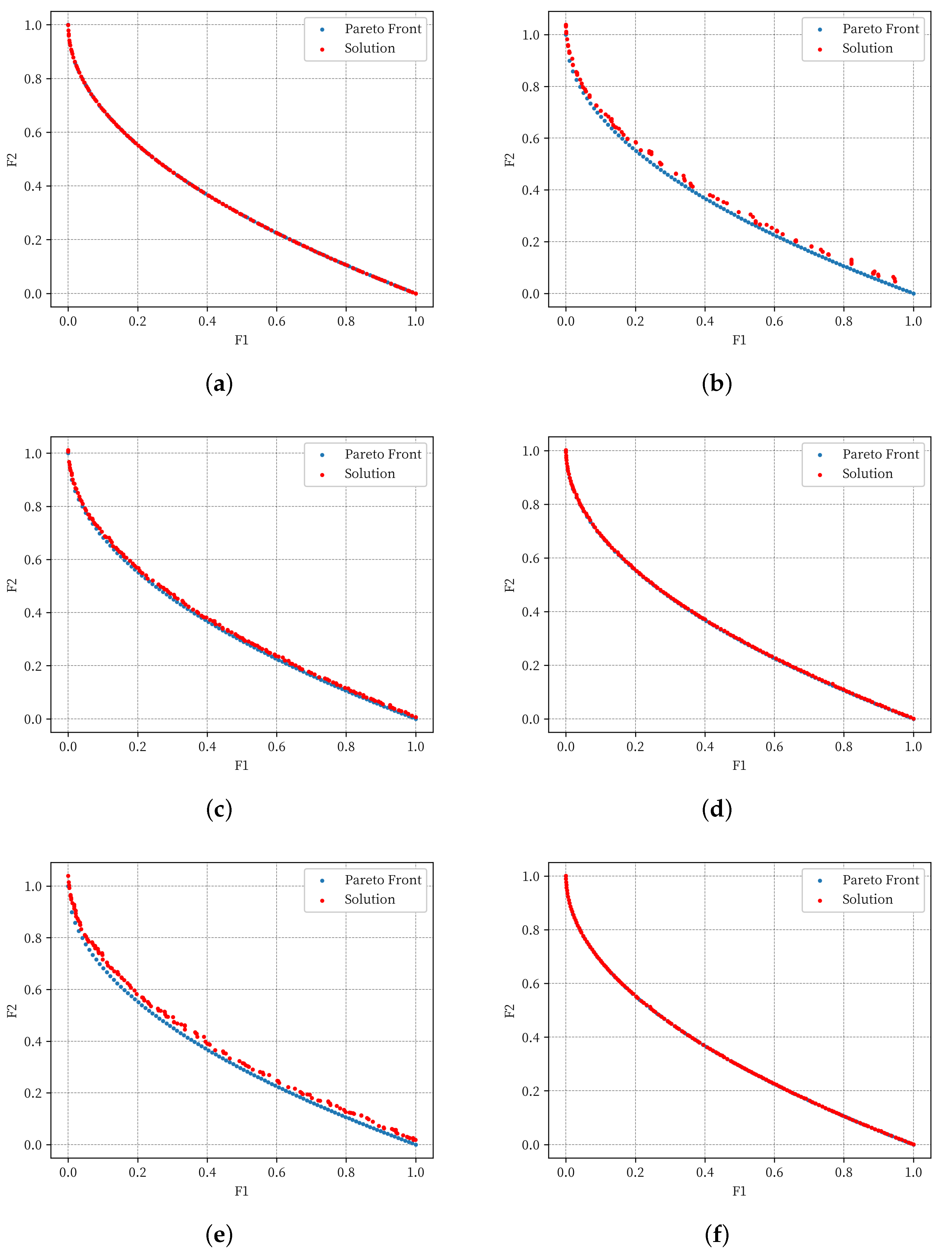
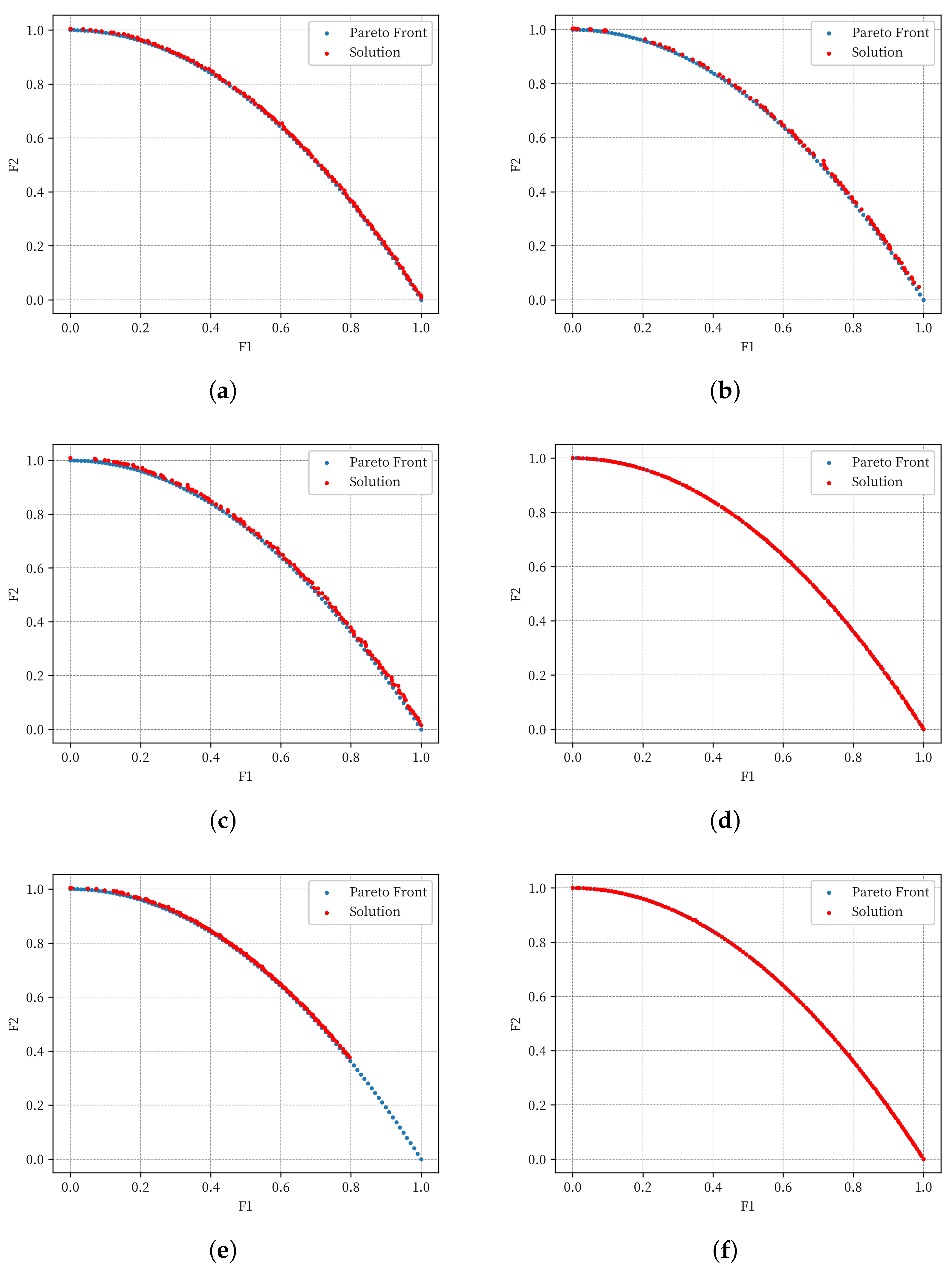
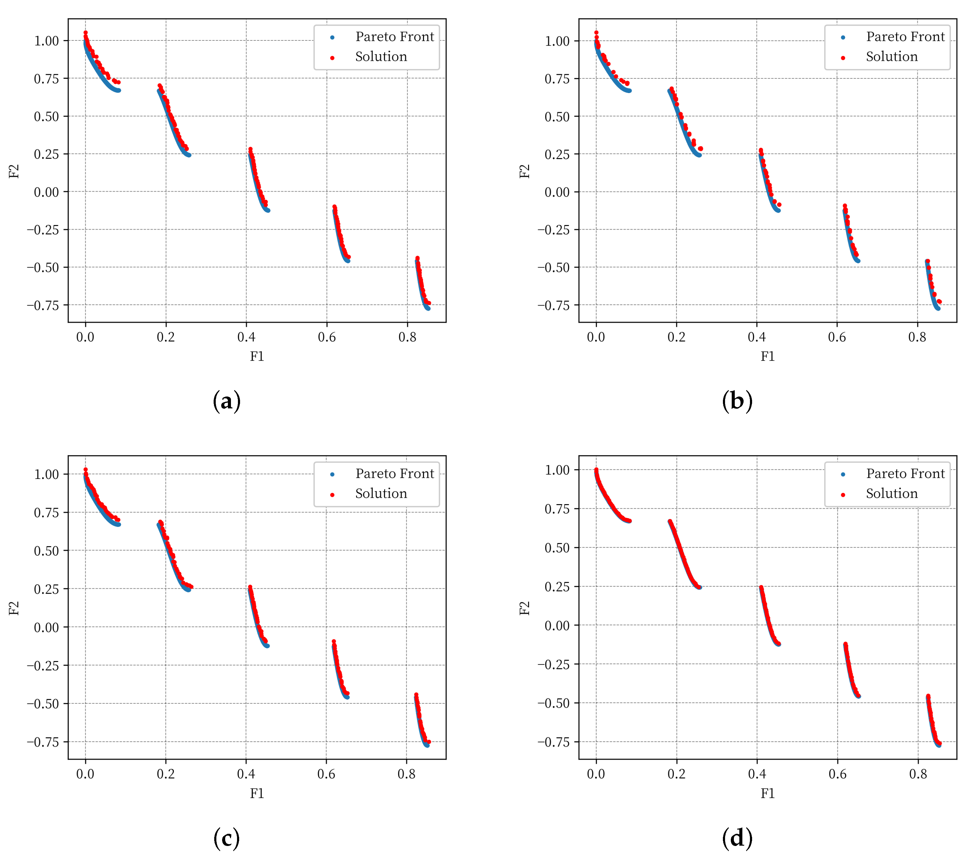
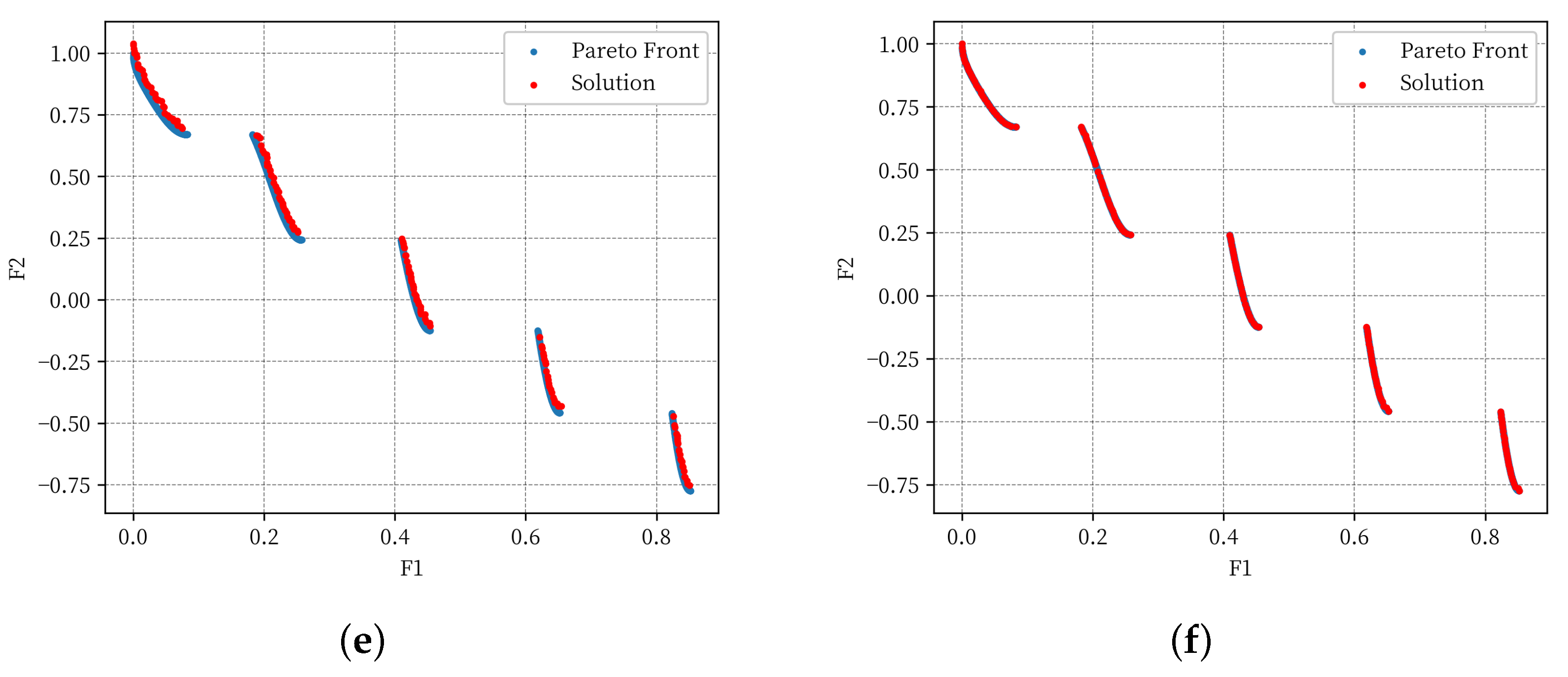
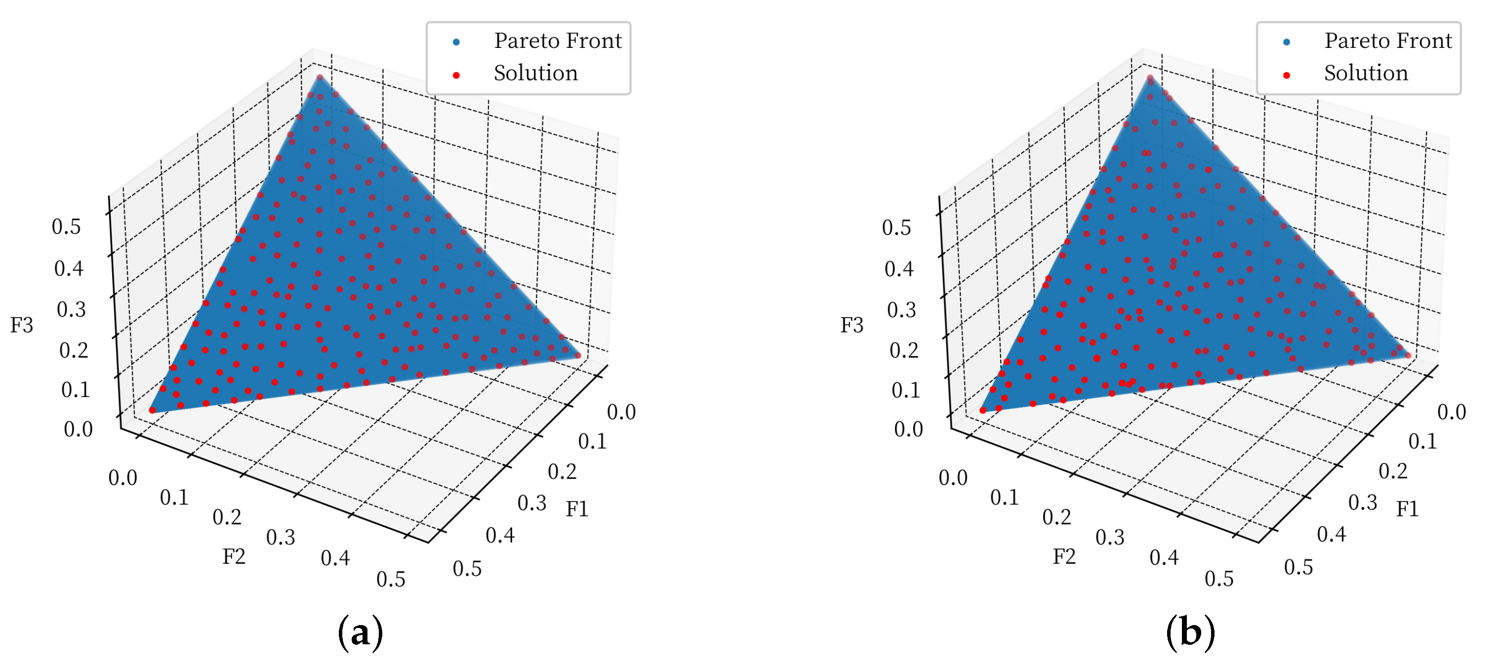
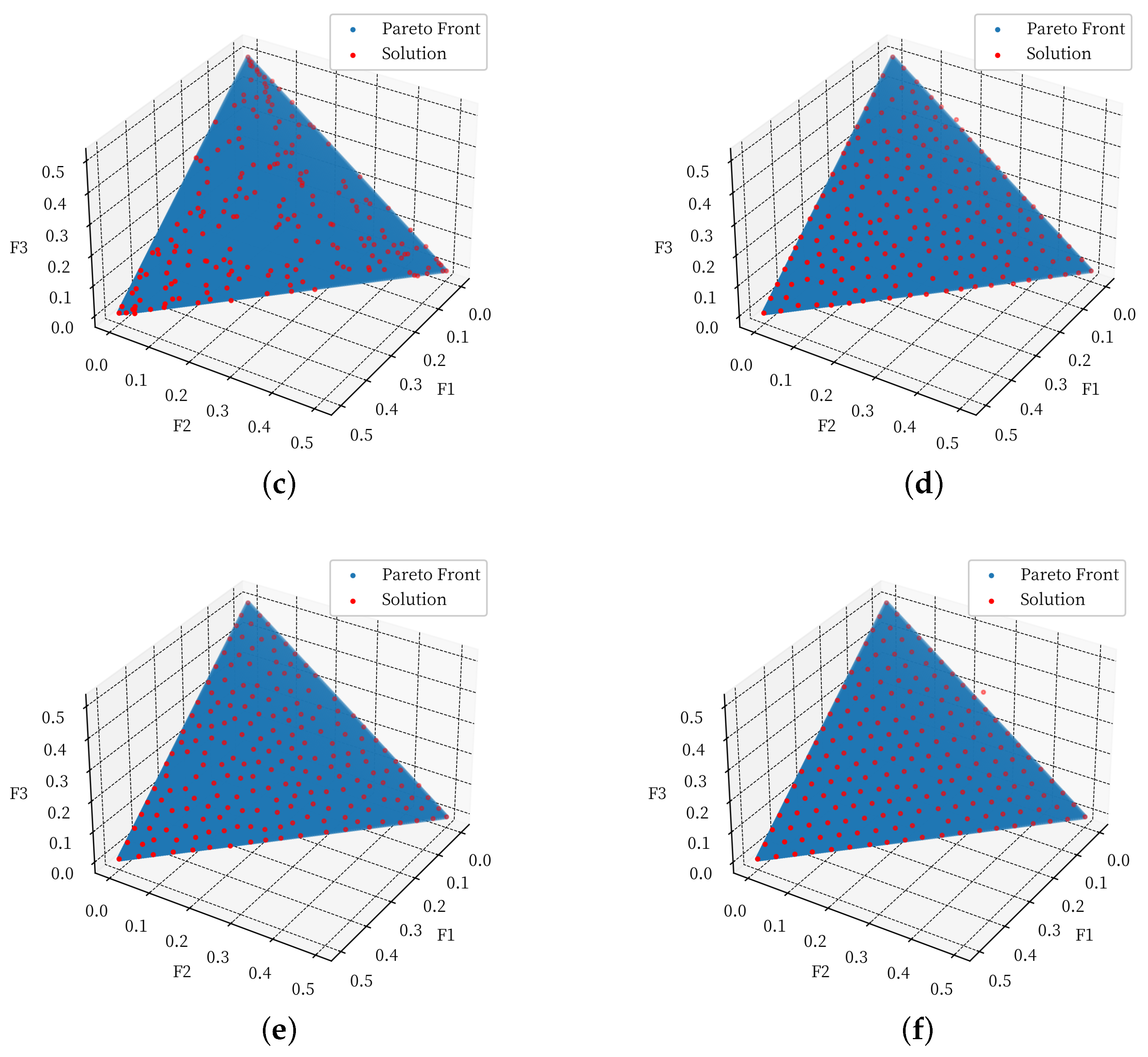
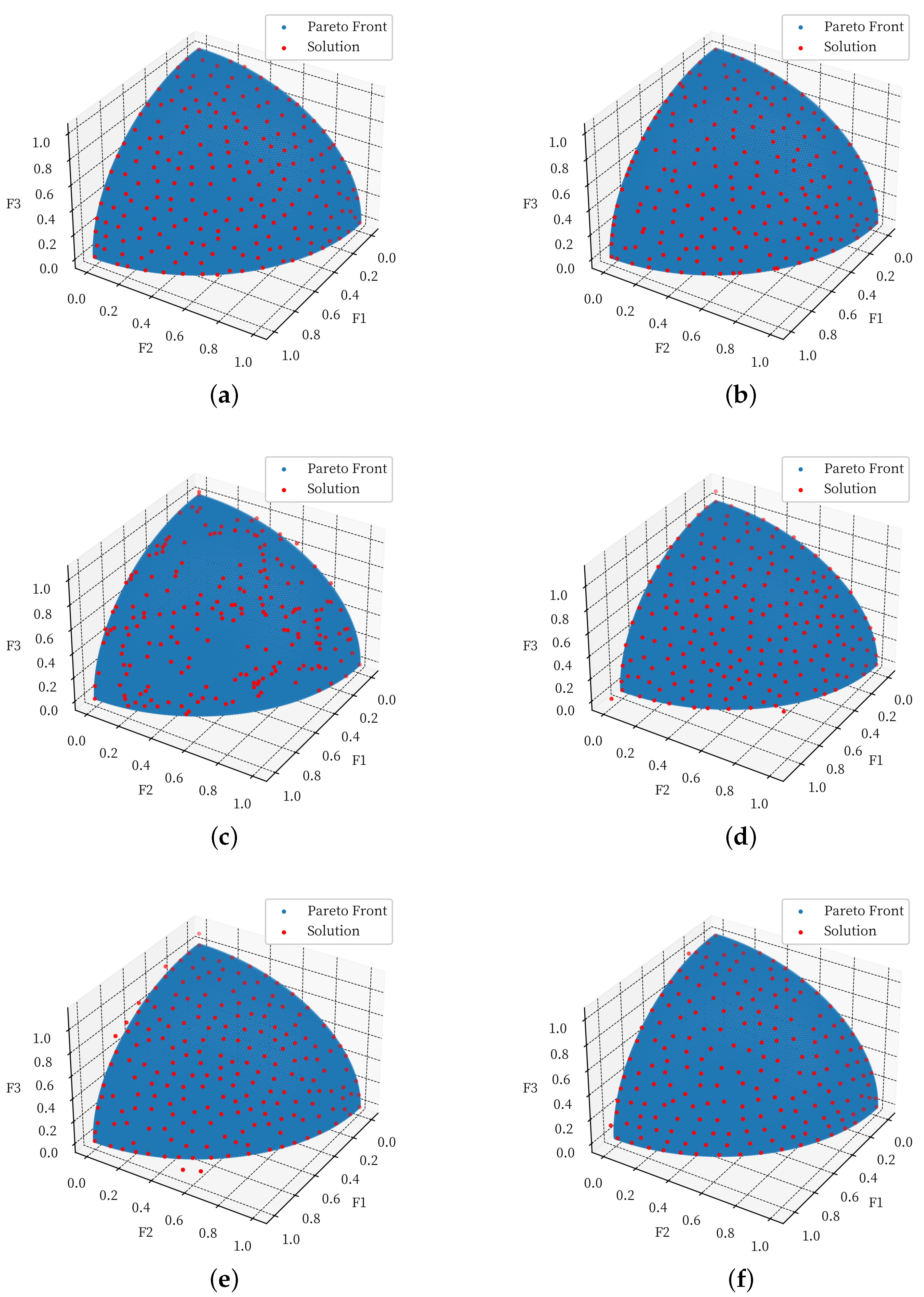
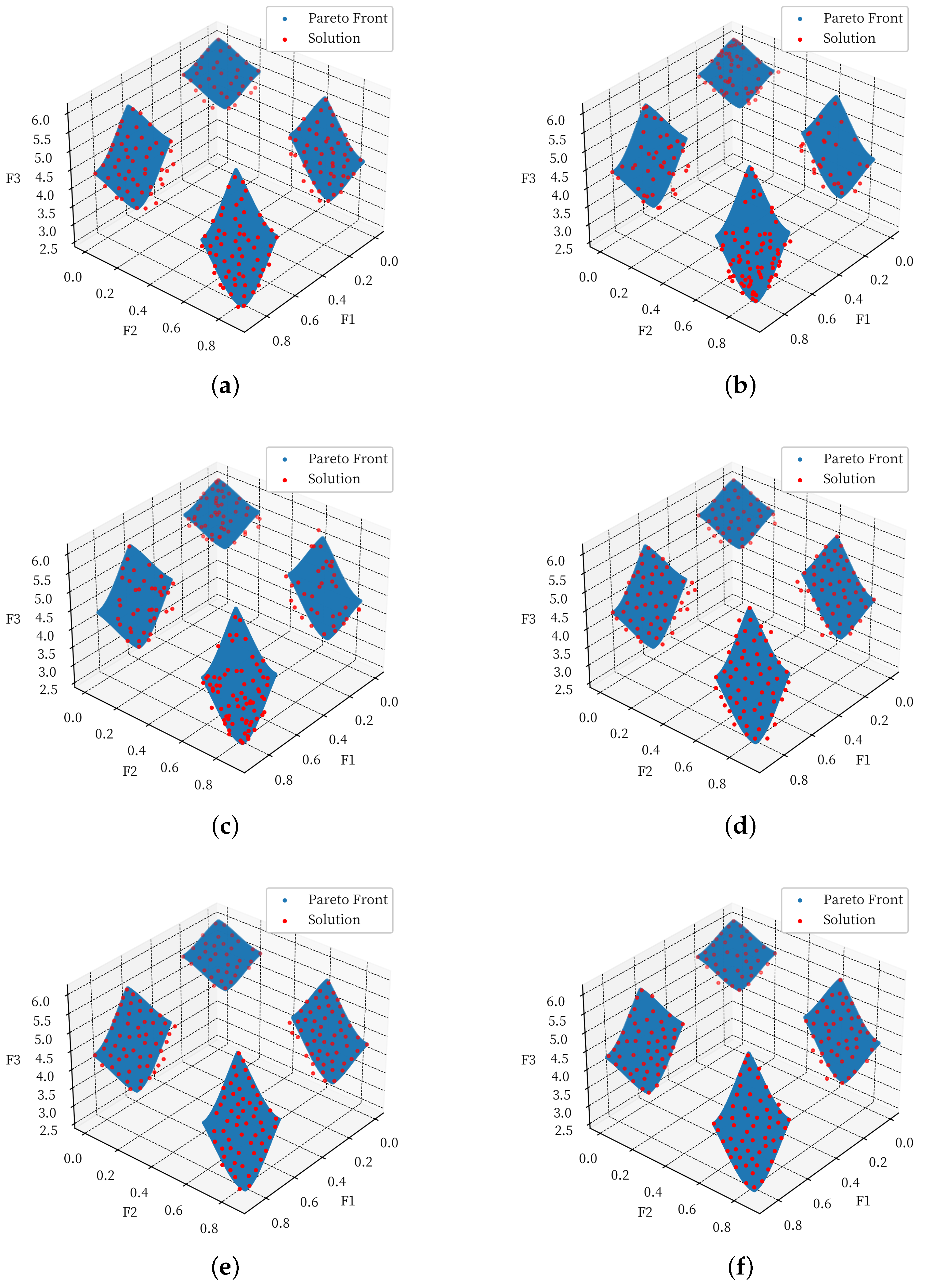
4.4. Results and Analysis

All experiments in this paper were independently run 30 times, and the mean and standard deviation of the experimental results were recorded. The Wilcoxon rank sum test with a significance level of 0.05 was used for the statistical analysis of the experimental results. The symbols “+”, “−” and “≈” indicate that the experimental results of another comparison algorithm are significantly better than, significantly worse than, or approximate to the experimental results of the MOEA/D-DPAW algorithm.

The results of IGD in six algorithms in this experiment on 12 two-objective test problems of ZDT and UF are shown in

Table 1. IGD values obtained by six algorithms about two-objective optimization problems on ZDT and UF.

	AGEMOEA	MOEA/D-URAW	NSGA-II-SDR	CMOPSO	MOEA/D-DAE	MOEA/D-DPAW
ZDT1	$4.5566\times {10}^{-3}$ $(6.87\times {10}^{-5})$ −	$2.4524\times {10}^{-2}$ $(1.77\times {10}^{-2})$ −	$6.9117\times {10}^{-3}$ $(5.58\times {10}^{-4})$ −	$2.7065\times {10}^{-3}$ $(5.07\times {10}^{-5})$ −	$3.9702\times {10}^{-3}$ $(5.41\times {10}^{-5})$ −	$2.6074\times {10}^{-3}$ $(2.84\times {10}^{-5})$
ZDT2	$4.5403\times {10}^{-3}$ $(8.37\times {10}^{-5})$ −	$2.5001\times {10}^{-2}$ $(2.13\times {10}^{-2})$ −	$7.1562\times {10}^{-3}$ $(6.65\times {10}^{-4})$ −	$2.6063\times {10}^{-3}$ $(2.18\times {10}^{-5})$ +	$3.8912\times {10}^{-3}$ $(4.80\times {10}^{-5})$ −	$2.6713\times {10}^{-3}$ $(3.75\times {10}^{-5})$
ZDT3	$5.7301\times {10}^{-3}$ $(1.25\times {10}^{-4})$ −	$1.5227\times {10}^{-2}$ $(5.57\times {10}^{-3})$ −	$7.3570\times {10}^{-3}$ $(5.29\times {10}^{-4})$ −	$4.6740\times {10}^{-3}$ $(5.97\times {10}^{-5})$ −	$3.0474\times {10}^{-3}$ $(2.20\times {10}^{-5})$ =	$3.0440\times {10}^{-3}$ $(3.07\times {10}^{-5})$
ZDT4	$4.4869\times {10}^{-3}$ $(7.35\times {10}^{-5})$ −	$1.9056\times {10}^{-1}$ $(1.17\times {10}^{-1})$ −	$1.7007\times {10}^0$ $(9.77\times {10}^{-1})$ −	$2.5600\times {10}^{-3}$ $(1.87\times {10}^{-5})$ =	$3.9801\times {10}^{-3}$ $(1.43\times {10}^{-4})$ −	$2.5614\times {10}^{-3}$ $(1.80\times {10}^{-5})$
ZDT6	$3.7375\times {10}^{-3}$ $(1.06\times {10}^{-4})$ −	$3.8146\times {10}^{-2}$ $(1.13\times {10}^{-2})$ −	$3.9215\times {10}^{-3}$ $(2.32\times {10}^{-4})$ −	$2.0549\times {10}^{-3}$ $(1.12\times {10}^{-5})$ +	$2.0538\times {10}^{-3}$ $(9.57\times {10}^{-6})$ +	$3.0974\times {10}^{-3}$ $(1.80\times {10}^{-5})$
UF1	$1.1084\times {10}^{-1}$ $(3.08\times {10}^{-2})$ −	$1.5812\times {10}^{-1}$ $(6.28\times {10}^{-2})$ −	$9.8125\times {10}^{-2}$ $(3.07\times {10}^{-2})$ −	$9.8281\times {10}^{-2}$ $(2.75\times {10}^{-2})$ −	$1.0932\times {10}^{-1}$ $(2.46\times {10}^{-2})$ −	$5.6112\times {10}^{-2}$ $(2.53\times {10}^{-2})$
UF2	$3.8838\times {10}^{-2}$ $(1.12\times {10}^{-2})$ −	$9.2979\times {10}^{-2}$ $(4.17\times {10}^{-2})$ −	$5.1230\times {10}^{-2}$ $(4.79\times {10}^{-3})$ −	$4.1317\times {10}^{-2}$ $(1.83\times {10}^{-2})$ −	$3.6030\times {10}^{-2}$ $(8.57\times {10}^{-3})$ −	$2.5671\times {10}^{-2}$ $(6.07\times {10}^{-3})$
UF3	$2.7212\times {10}^{-1}$ $(5.31\times {10}^{-2})$ −	$2.2370\times {10}^{-1}$ $(2.86\times {10}^{-2})$ =	$2.2401\times {10}^{-1}$ $(3.91\times {10}^{-2})$ =	$1.1325\times {10}^{-1}$ $(1.83\times {10}^{-2})$ +	$2.2560\times {10}^{-1}$ $(4.50\times {10}^{-2})$ =	$2.2389\times {10}^{-1}$ $(5.22\times {10}^{-2})$
UF4	$4.2069\times {10}^{-2}$ $(1.11\times {10}^{-3})$ =	$7.3622\times {10}^{-2}$ $(2.48\times {10}^{-3})$ −	$6.9834\times {10}^{-2}$ $(3.86\times {10}^{-3})$ −	$7.5978\times {10}^{-2}$ $(5.37\times {10}^{-3})$ −	$4.7901\times {10}^{-2}$ $(2.65\times {10}^{-3})$ −	$4.1958\times {10}^{-2}$ $(1.37\times {10}^{-3})$
UF5	$2.9557\times {10}^{-1}$ $(5.91\times {10}^{-2})$ +	$8.2835\times {10}^{-1}$ $(1.68\times {10}^{-1})$ −	$5.6403\times {10}^{-1}$ $(2.35\times {10}^{-1})$ −	$3.4625\times {10}^{-1}$ $(1.17\times {10}^{-1})$ =	$2.8012\times {10}^{-1}$ $(6.97\times {10}^{-2})$ +	$3.4526\times {10}^{-1}$ $(1.06\times {10}^{-1})$
UF6	$2.1861\times {10}^{-1}$ $(1.29\times {10}^{-1})$ −	$3.6294\times {10}^{-1}$ $(8.79\times {10}^{-2})$ −	$3.7128\times {10}^{-1}$ $(1.03\times {10}^{-1})$ −	$2.2384\times {10}^{-1}$ $(1.36\times {10}^{-1})$ −	$2.2171\times {10}^{-1}$ $(1.16\times {10}^{-1})$ −	$1.7370\times {10}^{-1}$ $(1.07\times {10}^{-1})$
UF7	$2.0336\times {10}^{-1}$ $(1.68\times {10}^{-1})$ −	$3.2097\times {10}^{-1}$ $(1.35\times {10}^{-1})$ −	$5.6390\times {10}^{-2}$ $(6.95\times {10}^{-3})$ +	$4.2142\times {10}^{-2}$ $(8.18\times {10}^{-2})$ +	$1.2998\times {10}^{-1}$ $(1.37\times {10}^{-1})$ =	$1.3069\times {10}^{-1}$ $(1.65\times {10}^{-1})$
+/−/≈	1/10/1	0/11/1	1/10/1	4/6/2	2/7/3

. According to the table, the MOEA/D-DPAW algorithm proposed in this paper has obtained the best IGD values on six test sets: ZDT1, ZDT3, UF1, UF2, UF4, and UF6. For the ZDT2 and ZDT4 problem, although the CMOPSO algorithm has the best solution effect, the IGD values calculated using the MOEA/D-DPAW algorithm are close to it. For the ZDT6, UF3, UF5, and UF7 problems, the performance of the MOEA/D-DPAW algorithm is slightly inferior to that of the MOEA/D-DAE and the CMOPSO algorithm. The results of HV in six algorithms in this experiment on 12 two-objective test problems of ZDT and UF are shown in

Table 2. HV values obtained by six algorithms about two-objective optimization problems on ZDT and UF.

	AGEMOEA	MOEA/D-URAW	NSGA-II-SDR	CMOPSO	MOEA/D-DAE	MOEA/D-DPAW
ZDT1	$7.1987\times {10}^{-1}$ $(7.12\times {10}^{-5})$ −	$6.9618\times {10}^{-1}$ $(1.11\times {10}^{-2})$ −	$7.1439\times {10}^{-1}$ $(9.20\times {10}^{-4})$ −	$7.2132\times {10}^{-1}$ $(1.10\times {10}^{-4})$ =	$7.2031\times {10}^{-1}$ $(8.91\times {10}^{-5})$ =	$7.2179\times {10}^{-1}$ $(4.37\times {10}^{-5})$
ZDT2	$4.4430\times {10}^{-1}$ $(8.86\times {10}^{-5})$ −	$4.1205\times {10}^{-1}$ $(2.49\times {10}^{-2})$ −	$4.3866\times {10}^{-1}$ $(1.07\times {10}^{-3})$ −	$4.4593\times {10}^{-1}$ $(9.49\times {10}^{-5})$ =	$4.4497\times {10}^{-1}$ $(6.43\times {10}^{-5})$ =	$4.4635\times {10}^{-1}$ $(4.39\times {10}^{-5})$
ZDT3	$5.9919\times {10}^{-1}$ $(3.56\times {10}^{-5})$ −	$6.0067\times {10}^{-1}$ $(9.53\times {10}^{-3})$ =	$5.9570\times {10}^{-1}$ $(9.80\times {10}^{-4})$ −	$6.0025\times {10}^{-1}$ $(2.00\times {10}^{-5})$ =	$5.9972\times {10}^{-1}$ $(3.38\times {10}^{-5})$ =	$6.0025\times {10}^{-1}$ $(2.86\times {10}^{-5})$
ZDT4	$7.1982\times {10}^{-1}$ $(1.51\times {10}^{-4})$ =	$4.9527\times {10}^{-1}$ $(1.25\times {10}^{-1})$ −	$1.1887\times {10}^{-2}$ $(3.91\times {10}^{-2})$ −	$7.2080\times {10}^{-1}$ $(3.77\times {10}^{-5})$ =	$7.1990\times {10}^{-1}$ $(5.28\times {10}^{-4})$ =	$7.2085\times {10}^{-1}$ $(3.91\times {10}^{-5})$
ZDT6	$3.8827\times {10}^{-1}$ $(9.93\times {10}^{-5})$ −	$3.3722\times {10}^{-1}$ $(1.49\times {10}^{-2})$ −	$3.8797\times {10}^{-1}$ $(2.28\times {10}^{-4})$ −	$3.8990\times {10}^{-1}$ $(1.42\times {10}^{-5})$ =	$3.8894\times {10}^{-1}$ $(2.64\times {10}^{-5})$ =	$3.8989\times {10}^{-1}$ $(2.05\times {10}^{-5})$
UF1	$5.9141\times {10}^{-1}$ $(3.37\times {10}^{-2})$ =	$5.3667\times {10}^{-1}$ $(4.43\times {10}^{-2})$ −	$5.9203\times {10}^{-1}$ $(3.11\times {10}^{-2})$ =	$6.4258\times {10}^{-1}$ $(2.07\times {10}^{-2})$ +	$5.9444\times {10}^{-1}$ $(3.18\times {10}^{-2})$ +	$5.9283\times {10}^{-1}$ $(2.48\times {10}^{-2})$
UF2	$6.8149\times {10}^{-1}$ $(7.27\times {10}^{-3})$ −	$6.4148\times {10}^{-1}$ $(2.14\times {10}^{-2})$ −	$6.5972\times {10}^{-1}$ $(5.73\times {10}^{-3})$ −	$6.8410\times {10}^{-1}$ $(5.82\times {10}^{-3})$ −	$6.8280\times {10}^{-1}$ $(9.50\times {10}^{-3})$ −	$6.9356\times {10}^{-1}$ $(4.70\times {10}^{-3})$
UF3	$4.2156\times {10}^{-1}$ $(4.92\times {10}^{-2})$ −	$3.7971\times {10}^{-1}$ $(2.83\times {10}^{-2})$ −	$4.3565\times {10}^{-1}$ $(4.95\times {10}^{-2})$ =	$5.5462\times {10}^{-1}$ $(2.84\times {10}^{-2})$ +	$4.5738\times {10}^{-1}$ $(4.15\times {10}^{-2})$ +	$4.3776\times {10}^{-1}$ $(4.94\times {10}^{-2})$
UF4	$3.8987\times {10}^{-1}$ $(9.88\times {10}^{-4})$ =	$3.3750\times {10}^{-1}$ $(4.01\times {10}^{-3})$ −	$3.5040\times {10}^{-1}$ $(4.93\times {10}^{-3})$ −	$3.4091\times {10}^{-1}$ $(6.96\times {10}^{-3})$ −	$3.8255\times {10}^{-1}$ $(2.35\times {10}^{-3})$ −	$3.9087\times {10}^{-1}$ $(1.46\times {10}^{-3})$
UF5	$2.2734\times {10}^{-1}$ $(6.03\times {10}^{-2})$ −	$1.1752\times {10}^{-2}$ $(3.67\times {10}^{-2})$ −	$3.7383\times {10}^{-2}$ $(4.51\times {10}^{-2})$ −	$2.2329\times {10}^{-1}$ $(7.19\times {10}^{-2})$ −	$1.9594\times {10}^{-1}$ $(8.21\times {10}^{-2})$ −	$2.3272\times {10}^{-1}$ $(5.43\times {10}^{-2})$
UF6	$3.0167\times {10}^{-1}$ $(7.36\times {10}^{-2})$ −	$1.8115\times {10}^{-1}$ $(5.64\times {10}^{-2})$ −	$1.3430\times {10}^{-1}$ $(7.64\times {10}^{-2})$ −	$3.0416\times {10}^{-1}$ $(6.17\times {10}^{-2})$ −	$2.9014\times {10}^{-1}$ $(8.92\times {10}^{-2})$ −	$3.2208\times {10}^{-1}$ $(6.49\times {10}^{-2})$
UF7	$4.6429\times {10}^{-1}$ $(1.17\times {10}^{-1})$ =	$3.2311\times {10}^{-1}$ $(8.29\times {10}^{-2})$ −	$5.0512\times {10}^{-1}$ $(1.25\times {10}^{-2})$ +	$5.3911\times {10}^{-1}$ $(6.15\times {10}^{-2})$ +	$4.4741\times {10}^{-1}$ $(1.18\times {10}^{-1})$ −	$4.6793\times {10}^{-1}$ $(9.88\times {10}^{-2})$
+/−/≈	0/8/4	0/11/1	1/9/2	3/4/5	2/5/5

. According to the table, The MOEA/D-DPAW algorithm proposed in this paper has obtained the best HV values on seven test sets: ZDT1, ZDT2, ZDT4, UF2, UF4, UF5, and UF6. For the ZDT3 and ZDT6 problem, the MOEA/D-URAW and the CMOPSO algorithms, respectively, obtain the best performances, but the results of the MOEA/D-DPAW algorithm are almost equal to them. For the UF1, UF3, and UF7 problems, the CMOPSO algorithm has the best performance. Although the MOEA/D-DPAW algorithm is not as good as the CMOPSO algorithm on those test problems, it still has excellent performance compared with other algorithms. Therefore, the MOEA/D-DPAW algorithm has excellent performance in solving the two-objective optimization problem, which proves the effectiveness of the improved strategy proposed in this paper, and the convergence and diversity of the solution set can be guaranteed.

The results of IGD in six algorithms in this experiment on 10 three-objective test problems of DTLZ and UF are shown in

Table 3. IGD values obtained by six algorithms about three-objective optimization problems on DTLZ and UF.

	AGEMOEA	MOEA/D-URAW	NSGA-II-SDR	CMOPSO	MOEA/D-DAE	MOEA/D-DPAW
DTLZ1	$2.0613\times {10}^{-2}$ $(2.27\times {10}^{-4})$ =	$1.5962\times {10}^{-1}$ $(1.70\times {10}^{-1})$ −	$1.5352\times {10}^0$ $(7.82\times {10}^{-1})$ −	$1.4187\times {10}^{-2}$ $(1.47\times {10}^{-4})$ +	$1.4106\times {10}^{-2}$ $(1.85\times {10}^{-4})$ +	$2.0733\times {10}^{-2}$ $(1.28\times {10}^{-4})$
DTLZ2	$5.2410\times {10}^{-2}$ $(1.20\times {10}^{-4})$ −	$5.4875\times {10}^{-2}$ $(1.16\times {10}^{-3})$ −	$7.0669\times {10}^{-2}$ $(2.59\times {10}^{-3})$ −	$3.8143\times {10}^{-2}$ $(4.62\times {10}^{-4})$ =	$5.5726\times {10}^{-2}$ $(4.67\times {10}^{-4})$ −	$3.8036\times {10}^{-2}$ $(2.77\times {10}^{-4})$
DTLZ3	$5.2694\times {10}^{-2}$ $(3.10\times {10}^{-4})$ +	$8.2878\times {10}^0$ $(4.99\times {10}^0)$ −	$6.8274\times {10}^{+1}$ $(2.11\times {10}^{+1})$ −	$5.8418\times {10}^0$ $(4.95\times {10}^0)$ +	$4.0454\times {10}^{-2}$ $(2.81\times {10}^{-3})$ +	$6.3007\times {10}^{-2}$ $(6.13\times {10}^{-3})$
DTLZ4	$5.2463\times {10}^{-2}$ $(1.25\times {10}^{-4})$ −	$2.1671\times {10}^{-1}$ $(2.33\times {10}^{-1})$ −	$6.8917\times {10}^{-2}$ $(2.04\times {10}^{-3})$ −	$4.1291\times {10}^{-2}$ $(7.46\times {10}^{-4})$ −	$5.6860\times {10}^{-2}$ $(9.63\times {10}^{-4})$ −	$3.8195\times {10}^{-2}$ $(3.76\times {10}^{-4})$
DTLZ5	$5.1969\times {10}^{-3}$ $(1.59\times {10}^{-4})$ −	$4.4681\times {10}^{-3}$ $(1.20\times {10}^{-4})$ −	$6.1547\times {10}^{-3}$ $(4.06\times {10}^{-4})$ −	$2.8355\times {10}^{-3}$ $(3.65\times {10}^{-4})$ −	$4.9753\times {10}^{-3}$ $(1.05\times {10}^{-4})$ −	$2.2375\times {10}^{-3}$ $(3.14\times {10}^{-5})$
DTLZ6	$4.8476\times {10}^{-3}$ $(6.32\times {10}^{-5})$ −	$3.7324\times {10}^{-2}$ $(1.70\times {10}^{-1})$ −	$5.7994\times {10}^{-3}$ $(3.30\times {10}^{-4})$ −	$2.0859\times {10}^{-3}$ $(1.65\times {10}^{-5})$ +	$2.0784\times {10}^{-3}$ $(1.44\times {10}^{-5})$ +	$4.6200\times {10}^{-3}$ $(1.03\times {10}^{-4})$
DTLZ7	$1.1606\times {10}^{-1}$ $(1.16\times {10}^{-1})$ −	$7.4706\times {10}^{-2}$ $(4.55\times {10}^{-3})$ −	$8.3862\times {10}^{-2}$ $(3.12\times {10}^{-3})$ −	$4.2191\times {10}^{-2}$ $(7.07\times {10}^{-4})$ −	$6.1264\times {10}^{-2}$ $(1.03\times {10}^{-3})$ −	$3.8302\times {10}^{-2}$ $(3.89\times {10}^{-4})$
UF8	$2.4862\times {10}^{-1}$ $(6.79\times {10}^{-2})$ −	$3.0642\times {10}^{-1}$ $(3.08\times {10}^{-2})$ −	$3.2636\times {10}^{-1}$ $(2.11\times {10}^{-2})$ −	$5.4976\times {10}^{-1}$ $(1.02\times {10}^{-1})$ −	$2.4558\times {10}^{-1}$ $(6.03\times {10}^{-2})$ −	$1.4738\times {10}^{-1}$ $(8.40\times {10}^{-2})$
UF9	$1.6155\times {10}^{-1}$ $(6.83\times {10}^{-2})$ =	$4.0613\times {10}^{-1}$ $(7.16\times {10}^{-2})$ −	$4.8438\times {10}^{-1}$ $(7.48\times {10}^{-2})$ −	$8.3236\times {10}^{-1}$ $(1.20\times {10}^{-1})$ −	$1.9118\times {10}^{-1}$ $(7.86\times {10}^{-2})$ −	$1.5937\times {10}^{-1}$ $(7.65\times {10}^{-2})$
UF10	$3.6358\times {10}^{-1}$ $(8.10\times {10}^{-2})$ =	$6.4174\times {10}^{-1}$ $(1.12\times {10}^{-1})$ −	$1.3944\times {10}^0$ $(3.92\times {10}^{-1})$ −	$3.3365\times {10}^0$ $(4.89\times {10}^{-1})$ −	$3.6439\times {10}^{-1}$ $(8.53\times {10}^{-2})$ =	$3.6367\times {10}^{-1}$ $(7.68\times {10}^{-2})$
+/−/≈	1/6/3	0/10/0	0/10/0	3/6/1	3/6/1

. According to the table, it can be seen that the MOEA/D-DPAW algorithm proposed in this paper obtained the best IGD values on the DTLZ2, DTLZ4, DTLZ5, DTLZ7, UF8, and UF9 test problems. For the UF10 problem, the AGEMOEA algorithm achieves the best solution, but the solution by the MOEA/D-DPAW algorithm is very close to it. For the problems of DTLZ1, DTLZ3, and DTLZ6, the performance of the MOEA/D-DAE algorithm is better. Although the performance of the MOEA/D-DPAW algorithm is inferior to that of the MOEA/D-DAE algorithm, it is still more outstanding compared with the remaining four algorithms. The results of HV in six algorithms in this experiment on nine three-objective test problems of DTLZ and UF are shown in

Table 4. HV values obtained by six algorithms about three-objective optimization problems on DTLZ and UF.

	AGEMOEA	MOEA/D-URAW	NSGA-II-SDR	CMOPSO	MOEA/D-DAE	MOEA/D-DPAW
DTLZ1	$8.4252\times {10}^{-1}$ $(3.47\times {10}^{-4})$ +	$5.3287\times {10}^{-1}$ $(3.11\times {10}^{-1})$ −	$3.4133\times {10}^{-3}$ $(1.68\times {10}^{-2})$ −	$8.5111\times {10}^{-1}$ $(5.83\times {10}^{-4})$ +	$8.5268\times {10}^{-1}$ $(2.90\times {10}^{-4})$ +	$8.4117\times {10}^{-1}$ $(3.90\times {10}^{-4})$
DTLZ2	$5.6175\times {10}^{-1}$ $(3.00\times {10}^{-4})$ −	$5.5715\times {10}^{-1}$ $(1.72\times {10}^{-3})$ −	$5.2251\times {10}^{-1}$ $(5.41\times {10}^{-3})$ −	$5.6387\times {10}^{-1}$ $(1.12\times {10}^{-3})$ −	$5.5815\times {10}^{-1}$ $(1.13\times {10}^{-3})$ −	$5.7376\times {10}^{-1}$ $(5.31\times {10}^{-4})$
DTLZ3	$5.5835\times {10}^{-1}$ $(2.08\times {10}^{-3})$ +	$5.1647\times {10}^{-1}$ $(4.31\times {10}^{-3})$ −	$5.3619\times {10}^{-1}$ $(3.27\times {10}^{-2})$ −	$5.5981\times {10}^{-2}$ $(1.71\times {10}^{-1})$ −	$5.7501\times {10}^{-1}$ $(8.29\times {10}^{-4})$ +	$5.5038\times {10}^{-1}$ $(7.16\times {10}^{-3})$
DTLZ4	$5.6182\times {10}^{-1}$ $(3.41\times {10}^{-4})$ −	$4.8870\times {10}^{-1}$ $(1.02\times {10}^{-1})$ −	$5.2749\times {10}^{-1}$ $(3.77\times {10}^{-3})$ −	$5.5911\times {10}^{-1}$ $(1.78\times {10}^{-3})$ −	$5.5728\times {10}^{-1}$ $(1.17\times {10}^{-3})$ −	$5.7348\times {10}^{-1}$ $(7.17\times {10}^{-4})$
DTLZ5	$1.9943\times {10}^{-1}$ $(1.98\times {10}^{-4})$ =	$1.9954\times {10}^{-1}$ $(2.00\times {10}^{-4})$ =	$1.9831\times {10}^{-1}$ $(3.61\times {10}^{-4})$ −	$2.0056\times {10}^{-1}$ $(2.48\times {10}^{-4})$ +	$2.0125\times {10}^{-1}$ $(3.16\times {10}^{-5})$ +	$1.9946\times {10}^{-1}$ $(1.10\times {10}^{-4})$
DTLZ6	$1.9985\times {10}^{-1}$ $(5.70\times {10}^{-5})$ =	$1.9142\times {10}^{-1}$ $(3.67\times {10}^{-2})$ −	$1.9949\times {10}^{-1}$ $(1.55\times {10}^{-4})$ =	$2.0142\times {10}^{-1}$ $(1.70\times {10}^{-5})$ +	$2.0143\times {10}^{-1}$ $(1.09\times {10}^{-5})$ +	$1.9995\times {10}^{-1}$ $(4.63\times {10}^{-5})$
DTLZ7	$2.7206\times {10}^{-1}$ $(1.44\times {10}^{-2})$ −	$2.6880\times {10}^{-1}$ $(2.11\times {10}^{-3})$ −	$2.5826\times {10}^{-1}$ $(2.08\times {10}^{-3})$ −	$2.8016\times {10}^{-1}$ $(7.92\times {10}^{-4})$ +	$2.8487\times {10}^{-1}$ $(3.11\times {10}^{-4})$ +	$2.7742\times {10}^{-1}$ $(8.43\times {10}^{-4})$
UF8	$3.5375\times {10}^{-1}$ $(4.38\times {10}^{-2})$ −	$3.1125\times {10}^{-1}$ $(3.26\times {10}^{-2})$ −	$2.0278\times {10}^{-1}$ $(2.86\times {10}^{-2})$ −	$1.7675\times {10}^{-2}$ $(1.73\times {10}^{-2})$ −	$3.5435\times {10}^{-1}$ $(4.49\times {10}^{-2})$ −	$4.1812\times {10}^{-1}$ $(6.58\times {10}^{-2})$
UF9	$6.4945\times {10}^{-1}$ $(6.08\times {10}^{-2})$ =	$4.0670\times {10}^{-1}$ $(5.48\times {10}^{-2})$ −	$2.6278\times {10}^{-1}$ $(7.22\times {10}^{-2})$ −	$2.7339\times {10}^{-2}$ $(3.36\times {10}^{-2})$ −	$6.2154\times {10}^{-1}$ $(7.11\times {10}^{-2})$ −	$6.5909\times {10}^{-1}$ $(6.73\times {10}^{-2})$
UF10	$2.1485\times {10}^{-1}$ $(7.62\times {10}^{-2})$ +	$2.7731\times {10}^{-2}$ $(3.04\times {10}^{-2})$ −	$2.0316\times {10}^{-1}$ $(5.27\times {10}^{-2})$ +	$1.9435\times {10}^{-1}$ $(7.34\times {10}^{-2})$ −	$1.9891\times {10}^{-1}$ $(6.79\times {10}^{-2})$ =	$1.9983\times {10}^{-1}$ $(7.43\times {10}^{-2})$
+/−/≈	3/4/3	0/9/1	1/8/1	4/6/0	5/4/1

. According to the table, the MOEA/D-DPAW algorithm proposed in this paper has obtained the best HV value on the four test problems of DTLZ2, DTLZ4, UF8, and UF9. The MOEA/D-DAE algorithm also obtained the best HV value for the DTLZ1, DTLZ3, DTLZ5, DTLZ6, and DTLZ7 problems, indicating the excellent performance of these two algorithms in solving three-objective optimization problems. From the perspective of data distribution, both the MOEA/D-DPAW algorithm and the MOEA/D-DAE algorithm have their advantages and disadvantages. Regarding the UF10 problem, the AGEMOEA algorithm achieved the best running results, and the MOEA/D-DPAW algorithm performed slightly worse than the AGEMOEA algorithm. Based on the above analysis, the MOEA/D-DPAW algorithm proposed in this paper also has a good performance when solving the three-objective optimization problem, and it can finally obtain the solution set with uniform distribution and a good convergence effect.

In order to display the operation results of the algorithm more intuitively, this paper selects three two-objective optimization problems, ZDT1, ZDT2, and ZDT3, three three-objective optimization problems DTLZ1, DTLZ4, and DTLZ7, with six representative MOPs altogether.

A comparison graph is drawn between the solution set obtained after the first run of six algorithms and the real Pareto front. Among them, the operation results of six algorithms on the ZDT1 problem are shown in Figure 3. It can be seen from the figure that the MOEA/D-DPAW algorithm proposed in this paper has the best convergence effect with the AGEMOEA algorithm and the CMOPSO algorithm, which almost completely fits the real Pareto front and has a good population distribution. The results show that the MOEA/D-DPAW algorithm has an excellent searching ability and weight vector adaptive adjustment strategy, and its enhanced neighborhood exploration mechanism can effectively guide the population to explore the Pareto front. In addition, the AGEMOEA algorithm and the CMOPSO algorithm have relatively low complexities and can be fully iterated, and so the final result is also excellent. The performance of the NSGA-II-SDR algorithm is the second, and there is some deficiency in the convergence. Moreover, the MOEA/D-URAW and the MOEA/D-DAE algorithms have the worst effects, and there is a significant gap between them and the other four algorithms in terms of convergence and diversity.

The results of six algorithms on the ZDT2 problem are shown in Figure 4. It can be seen from the figure that the MOEA/D-DPAW algorithm proposed in this paper has the best convergence effect with the CMOPSO algorithm and the highest degree of closeness to the real Pareto front, and the population has good diversity. The effectiveness of the dual-population is illustrated again, and the CMOPSO algorithm is based on the particle swarm optimization algorithm, which is also suitable for this problem. Among the other four comparison algorithms, their convergence is slightly worse than that of the MOEA/D-DPAW algorithm, and the population distribution is relatively dispersed. The population individuals obtained by the MOEA/D-URAW algorithm and the NSGA-II-SDR algorithm are obviously not evenly distributed. In the MOEA/D-DAE algorithm, the individuals in the final population are concentrated in the upper left part of the Pareto frontier, and the lower right part of the Pareto frontier becomes an unknown region that the algorithm failed to explore.

The results of six algorithms on the ZDT3 problem are shown in Figure 5. The real Pareto front of this problem is discrete distribution, which is more complex than the first two problems. As can be seen from the figure, the MOEA/D-DPAW algorithm proposed in this paper has the best convergence effect with the CMOPSO algorithm and the highest degree of closeness to the real Pareto front, and the population has good diversity. It shows that the improved strategy in the MOEA/D-DPAW algorithm is still effective, and that good results can be obtained when facing relatively complex MOPs. Among the other four comparison algorithms, their convergence is relatively worse than that of the MOEA/D-DPAW algorithm, the final population obtained by the MOEA/D-URAW algorithm is also relatively discrete, and the diversity is not fully guaranteed. Based on the above analysis, the effectiveness and superiority of the proposed MOEA/D-DPAW algorithm in solving two-objective optimization problems can also be intuitively seen.

The results of six algorithms on the DTLZ1 problem are shown in Figure 6. It can be seen from the figure that the performance of the MOEA/D-DPAW algorithm proposed in this paper is the best. This indicates that the advantages of the MOEA/D-DPAW algorithm are more obvious when facing high-dimensional MOPs, and that the enhanced neighborhood exploration mechanism can more effectively guide population individuals to search the Pareto front. Although the populations obtained via the other five comparison methods are also close to the true Pareto front, the distribution of individual populations is more dispersed than that of the MOEA/D-DPAW algorithm proposed in this paper. The population distribution effect obtained by the NSGA-II-SDR algorithm is the worst, while the population distribution obtained by the other four algorithms is significantly better than that obtained by the NSGA-II-SDR algorithm, but still inferior to the MOEA/D-DPAW algorithm.

The results of six algorithms on the DTLZ4 problem are shown in Figure 7. It can be seen from the figure that the convergence and diversity of the MOEA/D-DPAW algorithm proposed in this paper is better. This further demonstrates the effectiveness of the MOEA/D-DPAW algorithm in solving three-objective optimization problems. In the solution set obtained by the NSGA-II-SDR, CMOPSO, and MOEA/D-DAE algorithms, there are some individuals that are far away from Pareto front, and the convergence of the algorithm is weak. In addition, in the solution set obtained by the MOEA/D-URAW, NSGA-II-SDR, and MOEA/D-DAE algorithms, the distribution among individuals is not uniform enough to adequately maintain the diversity of the population.

The results of six algorithms on the DTLZ7 problem are shown in Figure 8. The real Pareto front of this problem is discretely distributed in three-dimensional space, which is more complex than the previous two problems. As can be seen from the figure, the MOEA/D-DPAW algorithm proposed in this paper and the MOEA/D-DAE algorithm have the best performances, and the population individuals can ensure convergence to the Pareto front and can have a relatively uniform distribution. This shows that in the face of complex high-dimensional MOPs, the weight vector adaptive adjustment strategy adopted in this paper can fit the actual Pareto front well, and enhancing the neighborhood search strategy can further improve the search ability of the algorithm, so that the population can finally obtain the best convergence effect. The effect of the AGEMOEA algorithm and the CMOPSO algorithm is second; there are some individuals far from Pareto front, and the convergence is worse than the MOEA/D-DPAW algorithm. The MOEA/D-URAW algorithm and the NSGA-II-SDR algorithm have the worst effects, which do not only converge to the Pareto front completely, but the distribution of population individuals will concentrate to within fixed areas, and the population diversity is not fully guaranteed. Based on the above analysis, the effectiveness and superiority of the proposed MOEA/D-URAW algorithm in solving the three-objective optimization problem can also be seen intuitively.

5. Conclusions

Aiming at the multi-objective optimization problem, this paper proposed an improved MOEA/D algorithm with a Dual-Population and Adaptive Weight strategy. In the algorithm, two different populations evolve according to their own standards; each uses its own advantages to exchange information, so as to further improve the performance of the solution. In addition, the weight vector adaptive adjustment strategy is used in the proposed algorithm to periodically change the weight vector in the evolution process, which makes the algorithm more suitable for solving MOPs with a complex Pareto front. At the same time, the enhanced neighborhood exploration mechanism is used to improve the local search ability of the algorithm, so as to avoid that the population individuals always focus on a specific area when facing the complex MOPs. The comparative experimental results on 22 standard test problems show that the algorithm proposed in this paper has a better solving accuracy and a better convergence effect, compared with many mainstream evolutionary multi-objective optimization algorithms in recent years when facing the two-objective optimization problems and three-objective optimization problems. Additionally, it can maintain the diversity of the individual population well, and population individuals can be distributed more evenly on the premise of being close to the real Pareto front.

In the future, based on the proposed algorithm in this paper, it can be extended to solving MOPs with higher dimensions, and exploring the performances of related strategies in more complex and high-dimensional spaces. Additionally, more attention should be paid to its effect in solving the parameter optimizations of practical problems.

References

1. Deb, K.; Pratap, A.; Agarwal, S.; Meyarivan, T. A fast and elitist multiobjective genetic algorithm: NSGA-II. IEEE Trans. Evol. Comput. 2002, 6, 182–197. [Google Scholar] [CrossRef] [Green Version]
2. Deb, K.; Jain, H. An evolutionary many-objective optimization algorithm using reference-point-based nondominated sorting approach, part I: Solving problems with box constraints. IEEE Trans. Evol. Comput. 2013, 18, 577–601. [Google Scholar] [CrossRef]
3. Yuan, M.; Li, Y.; Zhang, L.; Pei, F. Research on intelligent workshop resource scheduling method based on improved NSGA-II algorithm. Robot. Comput. Integr. Manuf. 2021, 71, 102141. [Google Scholar] [CrossRef]
4. Pan, L.; Xu, W.; Li, L.; He, C.; Cheng, R. Adaptive simulated binary crossover for rotated multi-objective optimization. Swarm Evol. Comput. 2021, 60, 100759. [Google Scholar] [CrossRef]
5. Yi, J.H.; Deb, S.; Dong, J.; Alavi, A.H.; Wang, G.G. An improved NSGA-III algorithm with adaptive mutation operator for Big Data optimization problems. Future Gener. Comput. Syst. 2018, 88, 571–585. [Google Scholar] [CrossRef]
6. Cui, Z.; Chang, Y.; Zhang, J.; Cai, X.; Zhang, W. Improved NSGA-III with selection-and-elimination operator. Swarm Evol. Comput. 2019, 49, 23–33. [Google Scholar] [CrossRef]
7. Gu, Z.M.; Wang, G.G. Improving NSGA-III algorithms with information feedback models for large-scale many-objective optimization. Future Gener. Comput. Syst. 2020, 107, 49–69. [Google Scholar] [CrossRef]
8. Sun, Y.; Yen, G.G.; Yi, Z. IGD indicator-based evolutionary algorithm for many-objective optimization problems. IEEE Trans. Evol. Comput. 2018, 23, 173–187. [Google Scholar] [CrossRef] [Green Version]
9. Hong, W.; Tang, K.; Zhou, A.; Ishibuchi, H.; Yao, X. A scalable indicator-based evolutionary algorithm for large-scale multiobjective optimization. IEEE Trans. Evol. Comput. 2018, 23, 525–537. [Google Scholar] [CrossRef]
10. Yuan, J.; Liu, H.L.; Ong, Y.S.; He, Z. Indicator-Based Evolutionary Algorithm for Solving Constrained Multiobjective Optimization Problems. IEEE Trans. Evol. Comput. 2021, 26, 379–391. [Google Scholar] [CrossRef]
11. Li, W.; Zhang, T.; Wang, R.; Ishibuchi, H. Weighted indicator-based evolutionary algorithm for multimodal multiobjective optimization. IEEE Trans. Evol. Comput. 2021, 25, 1064–1078. [Google Scholar] [CrossRef]
12. Li, H.R.; He, F.Z.; Yan, X.H. IBEA-SVM: An indicator-based evolutionary algorithm based on pre-selection with classification guided by SVM. Appl. Math. J. Chin. Univ. 2019, 34, 1–26. [Google Scholar] [CrossRef]
13. García, J.L.L.; Monroy, R.; Hernández, V.A.S.; Coello, C.A.C. COARSE-EMOA: An indicator-based evolutionary algorithm for solving equality constrained multi-objective optimization problems. Swarm Evol. Comput. 2021, 67, 100983. [Google Scholar] [CrossRef]
14. Zhang, Q.; Li, H. MOEA/D: A multiobjective evolutionary algorithm based on decomposition. IEEE Trans. Evol. Comput. 2007, 11, 712–731. [Google Scholar] [CrossRef]
15. Zhang, Y.; Wang, G.G.; Li, K.; Yeh, W.C.; Jian, M.; Dong, J. Enhancing MOEA/D with information feedback models for large-scale many-objective optimization. Inf. Sci. 2020, 522, 1–16. [Google Scholar] [CrossRef]
16. Cao, Z.; Liu, C.; Wang, Z.; Jia, H. An Improved MOEA/D Framework with Multoperator Strategies for Multi-objective Optimization Problems with a Large Scale of Variables. In Proceedings of the 2021 IEEE Congress on Evolutionary Computation (CEC), Kraków, Poland, 28 June–1 July 2021; pp. 2164–2170. [Google Scholar]
17. Wang, W.X.; Li, K.S.; Tao, X.Z.; Gu, F.H. An improved MOEA/D algorithm with an adaptive evolutionary strategy. Inf. Sci. 2020, 539, 1–15. [Google Scholar] [CrossRef]
18. Xie, Y.; Yang, S.; Wang, D.; Qiao, J.; Yin, B. Dynamic Transfer Reference Point-Oriented MOEA/D Involving Local Objective-Space Knowledge. IEEE Trans. Evol. Comput. 2022, 26, 542–554. [Google Scholar] [CrossRef]
19. Chen, L.; Pang, L.M.; Ishibuchi, H. New Solution Creation Operator in MOEA/D for Faster Convergence. In Proceedings of the International Conference on Parallel Problem Solving from Nature, Dortmund, Germany, 10–14 September 2022; Springer: Berlin/Heidelberg, Germany, 2022; pp. 234–246. [Google Scholar]
20. Zhang, Y.; He, L.; Yang, J.; Zhu, G.; Jia, X.; Yan, W. Multi-objective optimization design of a novel integral squeeze film bearing damper. Machines 2021, 9, 206. [Google Scholar] [CrossRef]
21. Akbari, V.; Naghashzadegan, M.; Kouhikamali, R.; Afsharpanah, F.; Yaïci, W. Multi-Objective Optimization of a Small Horizontal-Axis Wind Turbine Blade for Generating the Maximum Startup Torque at Low Wind Speeds. Machines 2022, 10, 785. [Google Scholar] [CrossRef]
22. Jiang, R.; Ci, S.; Liu, D.; Cheng, X.; Pan, Z. A hybrid multi-objective optimization method based on NSGA-II algorithm and entropy weighted TOPSIS for lightweight design of dump truck carriage. Machines 2021, 9, 156. [Google Scholar] [CrossRef]
23. Qi, Y.; Ma, X.; Liu, F.; Jiao, L.; Sun, J.; Wu, J. MOEA/D with adaptive weight adjustment. Evol. Comput. 2014, 22, 231–264. [Google Scholar] [CrossRef] [PubMed] [Green Version]
24. Tian, Y.; Cheng, R.; Zhang, X.; Jin, Y. PlatEMO: A MATLAB platform for evolutionary multi-objective optimization [educational forum]. IEEE Comput. Intell. Mag. 2017, 12, 73–87. [Google Scholar] [CrossRef] [Green Version]
25. Panichella, A. An adaptive evolutionary algorithm based on non-Euclidean geometry for many-objective optimization. In Proceedings of the GECCO ’19: Genetic and Evolutionary Computation Conference, Prague, Czech Republic, 13–17 July 2019; pp. 595–603. [Google Scholar]
26. Farias, L.R.; Araújol, A.F. Many-objective evolutionary algorithm based on decomposition with random and adaptive weights. In Proceedings of the 2019 IEEE International Conference on Systems, Man and Cybernetics (SMC), Bari, Italy, 6–9 October 2019; pp. 3746–3751. [Google Scholar]
27. Tian, Y.; Cheng, R.; Zhang, X.; Su, Y.; Jin, Y. A strengthened dominance relation considering convergence and diversity for evolutionary many-objective optimization. IEEE Trans. Evol. Comput. 2018, 23, 331–345. [Google Scholar] [CrossRef] [Green Version]
28. Zhang, X.; Zheng, X.; Cheng, R.; Qiu, J.; Jin, Y. A competitive mechanism based multi-objective particle swarm optimizer with fast convergence. Inf. Sci. 2018, 427, 63–76. [Google Scholar] [CrossRef]
29. Zhu, Q.; Zhang, Q.; Lin, Q. A constrained multiobjective evolutionary algorithm with detect-and-escape strategy. IEEE Trans. Evol. Comput. 2020, 24, 938–947. [Google Scholar] [CrossRef]
Figure 1. Research Roadmap of the Proposed Algorithm MOEA/D-DPAW.
Axioms 12 00100 g001
Figure 2. Framework of the Proposed Algorithm MOEA/D-DPAW.
Axioms 12 00100 g002
Figure 3. Comparison Between the Pareto Front and the Final Population Solution Set Obtained by the Six Different Algorithms on ZDT1 Test Problem Set. Subfigures (a) AGEMOEA, (b) MOEA/D-URAW, (c) NSGA-II-SDR, (d) CMOPSO, (e) MOEA/D-DAE, and (f) MOEA/D-DPAW correspond to the running results of algorithms AGEMOEA, MOEA/D-URAW, NSGA-II-SDR, CMOPSO, MOEA/D-DAE, and MOEA/D-DPAW, respectively.
Axioms 12 00100 g003
Figure 4. Comparison Between the Pareto Front and the Final Population Solution Set Obtained by the Six Different Algorithms on ZDT2 Test Problem Set. Subfigures (a) AGEMOEA, (b) MOEA/D-URAW, (c) NSGA-II-SDR, (d) CMOPSO, (e) MOEA/D-DAE, and (f) MOEA/D-DPAW correspond to the running results of algorithms AGEMOEA, MOEA/D-URAW, NSGA-II-SDR, CMOPSO, MOEA/D-DAE, and MOEA/D-DPAW, respectively.
Axioms 12 00100 g004
Figure 5. Comparison Between the Pareto Front and the Final Population Solution Set Obtained by the Six Different Algorithms on the ZDT3 Test Problem Set. Subfigures (a) AGEMOEA, (b) MOEA/D-URAW, (c) NSGA-II-SDR, (d) CMOPSO, (e) MOEA/D-DAE, and (f) MOEA/D-DPAW correspond to the running results of algorithms AGEMOEA, MOEA/D-URAW, NSGA-II-SDR, CMOPSO, MOEA/D-DAE, and MOEA/D-DPAW, respectively.
Axioms 12 00100 g005aAxioms 12 00100 g005b
Figure 6. Comparison Between the Pareto Front and the Final Population Solution Set Obtained by the Six Different Algorithms on DTLZ1 Test Problem Set. Subfigures (a) AGEMOEA, (b) MOEA/D-URAW, (c) NSGA-II-SDR, (d) CMOPSO, (e) MOEA/D-DAE, and (f) MOEA/D-DPAW correspond to the running results of algorithms AGEMOEA, MOEA/D-URAW, NSGA-II-SDR, CMOPSO, MOEA/D-DAE, and MOEA/D-DPAW, respectively.
Axioms 12 00100 g006aAxioms 12 00100 g006b
Figure 7. Comparison Between the Pareto Front and the Final Population Solution Set Obtained by the Six Different Algorithms on the DTLZ4 Test Problem Set. Subfigures (a) AGEMOEA, (b) MOEA/D-URAW, (c) NSGA-II-SDR, (d) CMOPSO, (e) MOEA/D-DAE, and (f) MOEA/D-DPAW correspond to the running results of algorithms AGEMOEA, MOEA/D-URAW, NSGA-II-SDR, CMOPSO, MOEA/D-DAE, and MOEA/D-DPAW, respectively.
Axioms 12 00100 g007
Figure 8. Comparison Between the Pareto Front and the Final Population Solution Set Obtained by the Six Different Algorithms on DTLZ7 Test Problem Set. Subfigures (a) AGEMOEA, (b) MOEA/D-URAW, (c) NSGA-II-SDR, (d) CMOPSO, (e) MOEA/D-DAE, and (f) MOEA/D-DPAW correspond to the running results of algorithms AGEMOEA, MOEA/D-URAW, NSGA-II-SDR, CMOPSO, MOEA/D-DAE, and MOEA/D-DPAW, respectively.
Axioms 12 00100 g008