SimuBP: A Simulator of Population Dynamics and Mutations Based on Branching Processes

Abstract

Originating from the Luria–Delbrück experiment in 1943, fluctuation analysis (FA) has been well developed to demonstrate random mutagenesis in microbial cell populations and infer mutation rates. Despite the remarkable progress in its theory and applications, FA often faces difficulties in the computation perspective, due to the lack of appropriate simulators. Existing simulation algorithms are usually designed specifically for particular scenarios, thus their applications may be largely restricted. There is a pressing need for more flexible simulators that rely on minimum model assumptions and are highly adaptable to produce data for a wide range of scenarios. In this study, we propose SimuBP, a simulator of population dynamics and mutations based on branching processes. SimuBP generates data based on a general two-type branching process, which is able to mimic the real cell proliferation and mutation process. Through simulations under traditional FA assumptions, we demonstrate that the data generated by SimuBP follow expected distributions, and exhibit high consistency with those generated by two alternative simulators. The most impressive feature of SimuBP lies in its flexibility, which enables the simulation of data analogous to real fluctuation experiments. We demonstrate the application of SimuBP through examples of estimating mutation rates.

1. Introduction

Fluctuation analysis (FA) is a classical approach for inferring mutation rates in microbial populations based on data collected from Luria–Delbrück (LD) experiments. A typical LD experiment is usually conducted by growing cells in parallel cultures and then plating the cultures on selective media to determine the number of mutants. Based on the data collected in parallel cultures, including the mutant counts and the total number of viable cells, estimation of the mutation rate can be performed based on appropriate mathematical models. During the long history of FA, various models (e.g., the Luria–Delbrück model, the Lea–Coulson model among many others) have been proposed and a great number of mutation rate estimators (based on moments, maximum likelihood, generating function, etc.) have been developed. The fundamental problem is to derive the distribution of the number of mutants at a given time (or population size), often called the LD distribution.

In contrast to the progress in mathematical modeling and statistical inference for the cell proliferation and mutation process, relatively less attention has been paid to computer simulations. As an important component of FA, computer simulation plays its unique role in the following aspects:

(1)

It provides a ground truth for evaluating the properties of mutation rate estimators, and for comparison between different methods;

(2)

It improves model calibration and interpretation by investigating deviations of simulated data from real experimental data;

(3)

It can be used to generalize model assumptions or get theoretically intractable solutions, which motivate new developments in theory;

(4)

The increasing computational resources make it possible to develop simulation-based estimators for mutation rate, which breaks the boundary of classical theory.

With the development of high-performance computing in recent years, intensive Monte Carlo simulations have become a powerful and financially feasible tool. This tool can be used to numerically elucidate the complex properties of evolutionary dynamics in microbial populations, which may be difficult to uncover by using mathematical approaches.

However, current simulation algorithms in the field of FA are still relatively underdeveloped. Existing simulators often rely on theoretical results derived from specific LD models, which, of course, require that a few assumptions be met. For example, one may draw samples directly from the LD distribution by applying the inverse transform to the cumulative distribution function (CDF), if it can be derived explicitly under certain conditions (e.g., deterministic growth of wild-type cells, no cell deaths or backward mutations). Another often used assumption in simulation is that the number of mutant cells can be represented as a nonhomogeneous filtered Poisson process (see Equation (2.2) in [1]). The heavy dependence on established results or model assumptions generates a dilemma for simulators in that, they can only generate data for particular cultivated models, not for the ones “outside the box”, whereas it is the latter, not the former, that actually needs more aid from simulation to imitate real experimental conditions and inspire new theories. If there was a simulator that requires a minimum set of assumptions and can be easily adapted to fit different models, it would greatly benefit the theoretical research in FA. Moreover, as stated in point (4) above, such a simulator also have potential implications in the methodology of newly-developed, data-oriented estimators of mutation rate.

In this study, we propose a flexible simulator, SimuBP, based on branching processes. SimuBP directly counts cell numbers at a given time in Monte Carlo simulations based on cell lifetime and offspring distributions, in a way that is analogous to the in vitro cell proliferation and mutation process. The main features of SimuBP include (i) it does not require any known results from the model, (ii) it is adaptable to different branching processes, and (iii) it can handle complex models such as cell deaths and backward mutations, different probabilistic behavior (lifetime and offspring distributions) for wild-type and mutant cells, time-varying mutations. For better dissemination, SimuBP is programmed using the open-source R language.

The rest of this article is organized as follows. In Section 2, we first provide a brief introduction to branching processes. We then present the SimuBP algorithm and introduce three simulation studies for validation, comparison, and demonstration purposes. Section 3 describes the details of the simulation procedures and summarizes the results, followed by discussion and conclusions in Section 4.

2. Methods

2.1. Discrete-Time, Continuous-Time Branching Processes, and Two-Type Branching Processes

Branching processes are commonly used to model an evolving population of microbial cells [2]. In general, cell reproduction can be described by the following Markov chain. Denote the population size of the nth cell generation (synchronized or not) by $X_n,n\ge 0$ with $X_0>0$, and the number of offspring of the ith cell of the $(n-1)$th generation by $Z_i$, the Markov chain $\{X_n,n\ge 0\}$ satisfies such a branching (or cell proliferation) rule

$$X_n=\sum _{i=1}^{X_{n-1}}{Z}_i,$$

where $Z_i,i=1,2,\cdots$ are non-negative, integer-valued, independent and identically distributed (i.i.d.) random variables following some discrete distribution (called the offspring distribution). Depending on whether the cell lifespan is fixed or random, branching processes can be categorized into discrete-time and continuous-time variants. For the discrete-time branching process (known as the Galton–Watson process or GWP [3]), the cell lifespan is assumed to be a constant, hence the cell birth events in each generation are synchronized. Such an assumption is relaxed in the continuous-time branching process by allowing the cell lifetime to vary as a continuous random variable. The branching process with cell lifespan following an arbitrary continuous distribution is called the age-dependent branching process or the Bellman-Harris process (BHP) [4,5]. In particular, when the cell lifetime distribution is i.i.d. exponential, the resulting process is called the Markov branching process (MBP) [6], otherwise, the corresponding continuous-time branching process is non-Markovian. It is obvious that, because of the branching rule, branching processes serve as appropriate mathematical models for cell population dynamics.

Since the Luria–Delbrück experiment is about random mutagenesis in cell populations, distinguishable cells with different probabilistic behavior should be allowed in the branching process model. For a typical fluctuation analysis involving two types of cells, namely the wild-type (non-mutant) and mutant cells, the population sizes of these two types of cells changing over time can be modeled by a two-type branching process [7]. The specific interest is in the distribution of mutant cell numbers at a given time, based on which the cell mutation probability (or mutation rate per cell division) can be inferred. Without loss of generality, let us consider a “General Two-Type Branching Process”, hereinafter abbreviated as GTBP, which satisfies the following two fundamental rules: (i) Each cell lives a certain time (fixed or random) and then splits into a random number of offspring, independent of other cells. In particular, we may allow the wild-type and mutant cells to have different lifetime distributions and different offspring distributions. The parameters of these two distributions determine the growth rates of the two types of cells; (ii) Upon cell division, each cell mutates with a certain constant probability, independent of the division times. In a general setting, we allow backward mutations and assume that wild-type and mutant cells have mutation probabilities ${\mu }_1$ and ${\mu }_2$, respectively, where $0\le {\mu }_1,{\mu }_2\le 1$. Note that, this GTBP should not be confused with the general branching process (also called the Crump-Mode-Jagers, or CMJ, process), which allows multiple birth events from each cell according to a point process [8,9]. We assume that the cell population starts from $y_0$ wild-type and $x_0$ mutant cells at $t=0$, and denote the time of plating (i.e., the time for cell counting) by $t_p$ and correspondingly the number of wild-type and mutant cells at $t_p$ by $y_t$ and $x_t$, respectively.

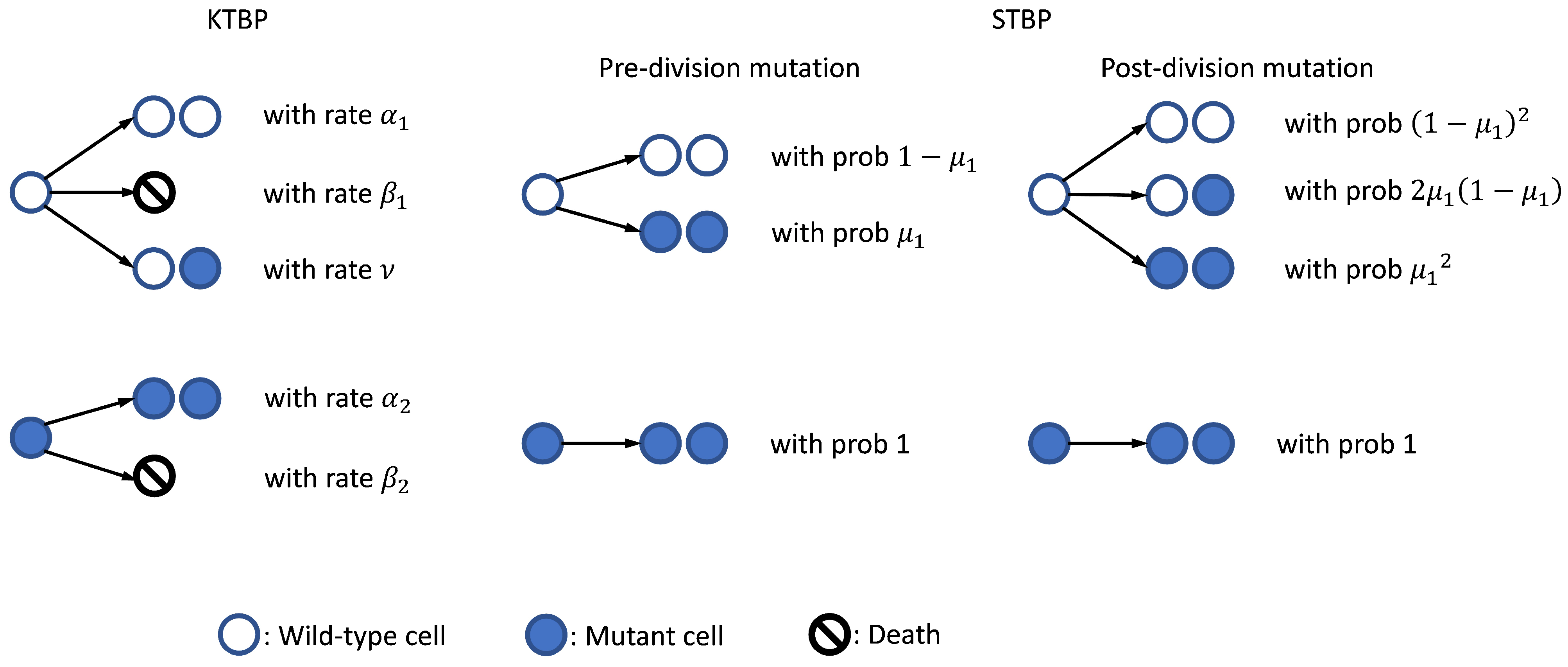
In contrast to the GTBP, we also define a “Simplified Two-Type Branching Process” (STBP) which is a special two-type MBP initiated by wild-type cell(s), with i.i.d. exponential lifetime for wild-type and mutant cells (i.e., non-differential growth) and binary-fission (i.e., Yule process), and without cell deaths or backward mutations. This model will be used throughout our simulation studies as described in Section 2.3. We note that the STBP is similar to Kendall’s two-type branching process (KTBP) [10], which is often known as the stochastic Luria–Delbrück model, with slight differences. The KTBP allows cell deaths and assumes that, upon division, each wild-type cell will either die, give birth to two wild-type offspring, or turn into one wild-type + one mutant cell, with certain rates; each mutant cell, on the other hand, will either die or divide into two mutant offspring with a certain rates [11]. However, in the STBP formulation, we assume all cells grow according to binary-fission with i.i.d. exponentially distributed lifetime, mutant cells always divide into two mutant offspring, and wild-type cells produce mutant offspring according to either pre- or post-division mutation. That is, for pre-division mutation, each wild-type cell will mutate with probability (${\mu }_1$, say) right before its division, but for post-division mutation, each wild-type cell will first divide into two wild-type offspring, then these two offspring will mutate independently with probability (${\mu }_1$) right after the division. In other words, from the wild-type cell perspective, the offspring distribution probability generating function (PGF) is $f\left(s\right)={\mu }_1+(1-{\mu }_1)s^2$ for pre-division mutation, and $f\left(s\right)={\mu }_1^2+2{\mu }_1(1-{\mu }_1)s+{(1-{\mu }_1)}^2{s}^2$ for post-division mutation. A schematic plot is shown in Figure 1 to illustrate cell mutations in the KTBP and STBP models.

2.2. Algorithm for Simulating Population Dynamics and Mutations Based on a GTBP

In the present study, we consider the GTBP defined above. Clearly, such a model is flexible enough to cover various branching processes, e.g., the GWP, the MBP, and the BHP, with mutations taken into account. Algorithm 1 shows the simulation procedure of SimuBP based on such a GTBP. As described in the algorithm, there are four input arguments passed to the R function SimuBP:

$$\mathrm{SimuBP}(\mathrm{bran}=\mathrm{list}(\mathrm{span},\mathrm{para},\mathrm{offd}), \mathrm{mupr}=\mathrm{c}({\mu }_1,{\mu }_2), \mathrm{n}0=\mathrm{c}(y_0,x_0), \mathrm{tp}),$$

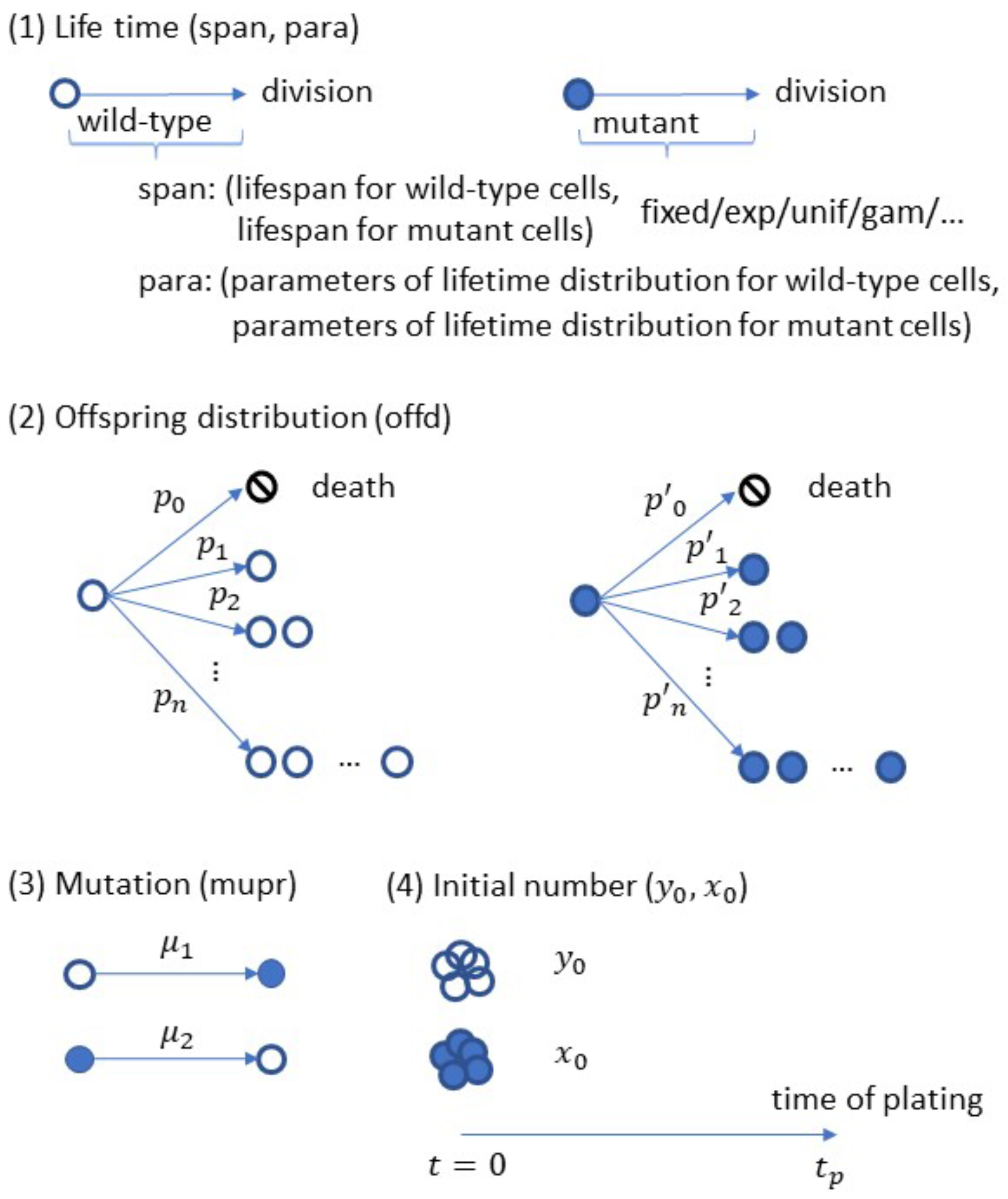
among which the first one “bran” (structured as an R list object) determines the branching rule of cell proliferation. In this list object, the “bran$span” component takes a character string, e.g., “fixed”, “exp”, “unif”, or “gam”, to specify the cell lifetime distribution (allowed to be different for wild-type and mutant cells). The “bran$para” component is a vector or matrix which provides the lifetime distribution parameters in a pair, for example, if “bran$span= ‘exp’ ”, then “bran$para= ‘c(1, 2)’ ” means the exponential rate parameter for wild-type cells is 1 and for mutant cells is 2. The third and last component “bran$offd” is a vector $(p_0,p_1,\cdots )$ specifying the offspring distribution, so “bran$offd= ‘c(0,0,2)’ ” means binary-fission (if necessary, the wild-type and mutant cells can have different offspring distributions by changing “bran$offd” to a matrix with two rows). The second input of the SimuBP function, “mupr=c(${\mu }_1,{\mu }_2$)”, is a vector specifying the forward and backward mutation probabilities. The third input vector, “n0=c($y_0,x_0$)”, specifies the initial number of wild-type and mutant cells. The last input “tp” is a scalar for the time of plating. Actually, both the time of plating and the population size at the time of plating can be used as input, however, considering the stochastic growth assumption of the GTBP, the former should be more appropriate for this simulator. For better illustration, these input arguments are shown in a schematic plot in Figure 2. The output of SimuBP is simply a vector $(z_t,x_t)$ where $x_t$ is the number of mutant cells at $t_p$ and $z_t=x_t+y_t$ is the total number of viable cells at $t_p$.

Algorithm 1 The SimuBP algorithm for simulating cell population with mutations based on a GTBP

Input: branching rule parameters including cell lifetime and offspring distributions (wild-type and mutant cells can have different parameters), mutation probability $({\mu }_1,{\mu }_2)$ for forward and backward mutations, initial cell number $(y_0,x_0)$, time of plating $t_p$ Output: total number of viable cells $z_t$ and number of mutant cells $x_t$ at $t_p$      Step 1. Initialize the number of wild-type and mutant cells at $t_p$ by setting $y_t=0,x_t=0$. Step 2. Generate two vectors ${\overrightarrow{T}}_1,{\overrightarrow{T}}_2$ from the specified lifetime distribution. ${\overrightarrow{T}}_1$ and ${\overrightarrow{T}}_2$ are of length $y_0$ and $x_0$, denoting the lifetime of wild-type and mutant cell(s) in the first (or current) generation. Generate two binary vectors ${\overrightarrow{\delta }}_1,{\overrightarrow{\delta }}_2$ from $\mathrm{Bern}\left({\mu }_1\right)$ and $\mathrm{Bern}\left({\mu }_2\right)$. ${\overrightarrow{\delta }}_1$ and ${\overrightarrow{\delta }}_2$ are of length $y_0$ and $x_0$, indicating whether mutation occurs for the wild-type and mutant cell(s) in the first (or current) generation. Based on ${\overrightarrow{T}}_1,{\overrightarrow{T}}_2$ and ${\overrightarrow{\delta }}_1,{\overrightarrow{\delta }}_2$, calculate the accumulated lifetimes ${\overrightarrow{T}}_w,{\overrightarrow{T}}_m$ for wild-type and mutant cells. Step 3. Count wild-type cells with $T_w<t_p$ and denote this number by $n_w$, these wild-type cells will continue to divide. Count wild-type cells with $T_w\ge t_p$ and denote this number by $y_w$, update $y_t=y_t+y_w$. Similarly, count mutant cells with $T_m<t_p$ and denote this number by $n_m$, count mutant cells with $T_m\ge t_p$ and denote this number by $x_w$, update $x_t=x_t+x_w$. Let $z_t=y_t+x_t$. while  $n_w+n_m>0$  do     (a) Based on the offspring distribution(s), generate the numbers of offspring for the wild-type and mutant cells in current generation.     (b) Repeat Steps 2∼3 by updating $y_0$ and $x_0$ with the numbers of offspring in (a). As cell division/mutation continues along generations, $n_w$ and $n_m$ decrease and the sum eventually reaches 0 to quit the loop. end while

2.3. Simulation Studies for Validation, Comparison, and Demonstration

We perform simulation studies based on an STBP to evaluate the performance of SimuBP, including three components S1∼S3 with the following specific aims:

S1:

To check goodness-of-fit (GoF) of the STBP model to the data generated by SimuBP.

S2:

To compare the data generated by SimuBP with those by two alternative simulators.

S3:

To demonstrate mutation rate estimation based on the data generated by SimuBP.

Simulation S1 focused on validating the simulated data by SimuBP based on the STBP model. Suppose that, in the STBP the exponential rate of the cell lifetime distribution is a, and the mutation probability of the wild-type cell is $\mu$. Two different cases, S1a and S1b, are considered depending on the initial number of wild-type cells: $y_0=1$ and $y_0>1$. Denote the random variable of the total number of viable cells at the time of plating $t_p$ by $Z_t$, and the random variable of the number of wild-type cells at $t_p$ by $Y_t$. For S1a: $y_0=1$, the distributions of $Z_t$ and $Y_t$ can be obtained explicitly by using the property of binary-fission MBP [12] (for convenience, a brief derivation is provided in Appendix A.1):

$$Z_t\sim \mathrm{geo}\left(e^{-a{t}_p}\right),$$

(1)

and

$$Y_t\sim \mathrm{geo}\left(\frac{1-2\mu }{(1-\mu )exp\left(a(1-2\mu )t_p\right)-\mu }\right).$$

(2)

When $\mu$ is small as in typical fluctuation experiments, Formula (2) can be approximated by

$$Y_t\sim \mathrm{geo}\left(e^{-a(1-2\mu )t_p}\right).$$

(3)

Consequently, for S1b: $y_0>1$,

$$Z_t|y_0\sim \mathrm{negbin}(y_0,e^{-a{t}_p}),$$

(4)

and

$$Y_t|y_0\sim \mathrm{negbin}(y_0,e^{-a(1-2\mu )t_p}).$$

(5)

We then use SimuBP with properly specified input arguments to generate data $(z_t,y_t)$ based on the STBP, and check the GoF of these data to the above theoretical distributions. Note that, since forward simulation is generally not efficient, to avoid slow computation, SimuBP does not simply apply superposition (via looping) of the $y_t$ and $x_t$ counts initiated by a single cell, but rather generates $y_t$ and $x_t$ samples directly from non-unit $y_0$ (and $x_0$ as well in a generalized setting).

It is worth noting that, this STBP is different from the traditional Luria–Delbrück or Lea–Coulson model because it assumes stochastic growth for both wild-type and mutant cells. To illustrate this point, we perform an additional simulation study S1c, where the $z_t$ and $y_t$ counts are generated from SimuBP according to the STBP used above. The distribution of the number of mutants $x_t=z_t-y_t$ is then calculated and compared with a corresponding LD distribution to check the GoF.

Simulation S2 is conducted to compare SimuBP with two other simulation algorithms. Both Algorithms 2 and  3 simulate counts of $z_t$ and $x_t$ based on the STBP model. Algorithm 2 comprises four steps: First, obtain the occurring time of each cell division event prior to plating. This is done by using the distribution of the interarrival times of binary-fission MBP (see Proposition 1 in [13]). Second, count the population size resulting from each initial cell and sum up across the $z_0$ initial cells to obtain $z_t$. Third, determine among all cell division events the ones corresponding to mutation events, and consequently calculate for each mutation event its excess time until plating. Last, generate the resulting number of mutant cells from each mutation and sum up across the mutation events to obtain $x_t$. We denote the simulation study comparing Algorithms 1 and 2 by S2a.

Algorithm 2 Alternative simulator based on an STBP

Input: exponential rates $a_1,a_2$ for wild-type and mutant cell life times, initial number of cells (wild-type) $z_0$, mutation probability $\mu$, time of plating $t_p$ Output: total number of viable cells $z_t$ and number of mutant cells $x_t$ at $t_p$      Step 1. For each initial wild-type cell, calculate the occurring times of the successive division events along its genealogy until $t_p$ by generating and summing up the exponentially distributed interarrival times with rate $j{a}_1,j=1,2,\cdots$. Denote the occurring times starting from the ith initial cell by $\left\{S_i\right\}$. Step 2. Count the number of elements in $\left\{S_i\right\}$ by $n_i$. Because of the binary-fission property, the population size at $t_p$, initiated by the ith cell is $(n_i+1)$, hence $z_t={\sum }_{i=1}^{z_0}(n_i+1)$. Step 3. Determine whether each cell division incurs mutation by generating $(z_t-z_0)$ random numbers from $\mathrm{Bern}\left(\mu \right)$. Denote the number of mutations by m which is two times (This number may vary depending on the assumption of pre- or post-division mutations.) the sum of the $(z_t-z_0)$ Bernoulli random numbers. Denote the occurring time of the ith mutation event by $t_i,1\le i\le m$, so its excess time until plating is $t_p-t_i$. Step 4. For each mutation, generate its resulting mutant cell count at $t_p$ from shifted geometric distribution $\mathrm{geo}\left(e^{-a_2(t_p-t_i)}\right)+1$, and finally sum up across all m mutant cell counts to get the total number of mutant cells $x_t$ at $t_p$.

In the second part of Simulation S2, denoted by S2b, we compare SimuBP with another simulator (Algorithm 3) adapted from the software SALVADOR [14]. Algorithm 3 differs from SALVADOR mainly in that it generates the number of wild-type cells $z_t$ at the time of plating from geometric growth rather than treating $z_t$ as input, and replaces the Poisson distributed number of mutations based on deterministic growth by the actual number of mutations based on stochastic growth. These adaptions make it easier to compare Algorithm 3 with Algorithms 1 or 2. It can be seen that Algorithms 2 and 3 are closely related and both rely on the exponential lifetime assumption so that once the number of mutations and the time from each mutation to plating are determined, the number of mutant cells $x_t$ at the time of plating can be obtained by generating geometrically distributed (with shift) random numbers.

Algorithm 3 Alternative simulator adapted from SALVADOR [14]

Input: exponential rates $a_1,a_2$ for wild-type and mutant cell life times, initial number of cells (wild-type) $z_0$, mutation probability $\mu$, time of plating $t_p$ Output: total number of viable cells $z_t$ and number of mutant cells $x_t$ at $t_p$      Step 1. Generate the population size $z_t$ at $t_p$ by summing up $z_0$ random numbers, each drawn from $\mathrm{geo}\left(e^{-a_1{t}_p}\right)$. Step 2. Calculate the total number of mutations by $m=\mu ·z_t$, and generate the occurring time $t_i$ of the ith mutation event, $1\le i\le m$, from truncated, flipped exponential distribution with range $[0,t_p]$, i.e., from CDF $F\left(t\right)=\frac{e^{a_{1}t}-1}{e^{a_1{t}_p}-1},0\le t\le t_p$. This is done by simulating $t_i$ as $[log(u(e^{a_1{t}_p}-1)+1)]/a_1$ where the random number $u\sim \mathrm{unif}(0,1)$. Step 3. For each mutation, generate its resulting mutant cell count at $t_p$ from shifted geometric distribution $\mathrm{geo}\left(e^{-a_2(t_p-t_i)}\right)+1$, and finally sum up across all m mutant cell counts to get the total number of mutant cells $x_t$ at $t_p$.

It should be emphasized that, SimuBP is flexible to generate more general fluctuation experimental data than most of the other simulators including Algorithms 2 and 3, for instance, by allowing

(1)

the cell lifetime to follow an arbitrary continuous distribution, or be a constant,

(2)

the offspring distribution to be any discrete distribution, not just binary-fission,

(3)

cell deaths and backward mutations,

(4)

the initial cell population to contain both wild-type and mutant cells.

Moreover, SimuBP can be further extended to simulate other complex mutation processes governed by non-constant (e.g., piece-wise constant or even time-varying) mutation rate, as seen in the second example of the following demonstrations.

Lastly, we demonstrate the application of SimuBP through Simulation S3 of estimating mutation rates in a two-type MBP via two examples, S3a and S3b. In Simulation S3a, we first generate data from SimuBP based on the STBP model and then perform point estimation for the mutation probability by using the MOM/MLE estimator proposed in [12]. Example S3b considers the case of two-stage mutations, that is, during cell proliferation, mutations occur at a constant rate in stage 1 and, when entering stage 2 switch to another constant rate. Such data may be observed in fluctuation experiments comprising abrupt changes in external conditions. A typical example can be found in the protocol of mutagenesis experiment on E. coli under sub-inhibitory antibiotic stress [15], which introduces a cell recovery step prior to plating. The mutation rate in this two-stage process is a piece-wise constant function, which can be easily incorporated by SimuBP, but not by any other simulators. We then estimate the three unknown parameters of the piece-wise constant mutation rate function by using an estimator proposed in [16] based on approximate Bayesian computation. The estimation results of the three parameters are shown by a heatmap of the joint posterior samples of Markov chain Monte Carlo (MCMC).

3. Results

3.1. Validation of Simulated Data Based on a STBP

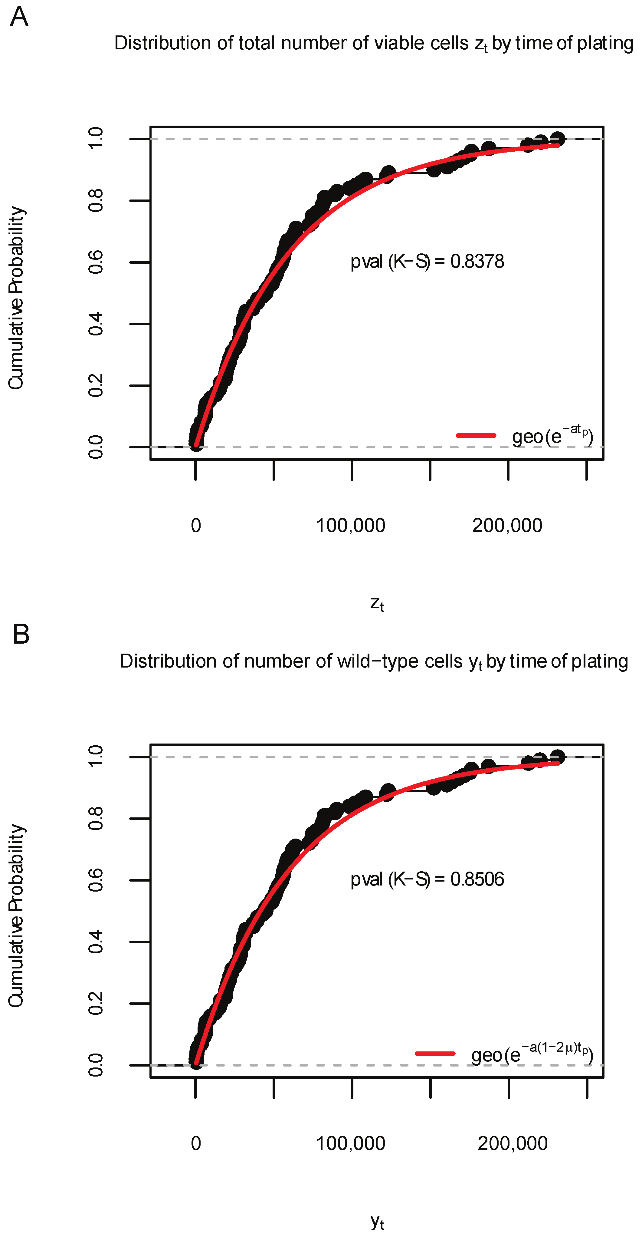
For Simulation S1a where $y_0=1$, the input of SimuBP was configured such that the cell lifetime follows an exponential distribution with rate 1 (for wild-type cells) and 1 (for mutant cells), the offspring distribution is binary-fission, i.e., with PGF $f\left(s\right)=s^2$, the mutation probabilities ${\mu }_1=2\times {10}^{-4}$ (forward mutation) and ${\mu }_2=0$ (backward mutation), the initial cell numbers $y_0=1,x_0=0$, and the time of plating $t_p=11$. Repeating the simulation 100 times, we plotted the empirical cumulative distribution function (ECDF) of the 100 samples of $z_t$ and $y_t$ in Figure 3, together with the theoretical CDF curves obtained from Formulae (1) and (3). The GoF of the theoretical CDFs to the simulated data was evaluated by a Kolmogorov–Smirnov (K-S) test and the p-value was shown beside the curves. In addition, the above procedure was repeated 1000 times to check the average GoF. Based on the 1000 K-S test p-values, we obtained the proportions of significant K-S tests: 0.046 and 0.045, for the distribution of $z_t$ and $y_t$ samples, respectively.

Simulation S1b ($y_0>1$) was conducted using similar settings, except that the initial cell numbers were set to $y_0=10,x_0=0$. The corresponding distribution plots based on 100 samples of $z_t$ and $y_t$ were shown in Figure 4, and the proportions of significant p-values among 1000 K-S tests are 0.053 (for $z_t$) and 0.053 (for $y_t$). These results show that SimuBP does generate data according to the STBP model as expected.

In Simulation S1c, we considered the non-differential growth case of the LD distribution and set its parameters as follows: the growth rate ${\beta }_1=1$ for both wild-type and mutant cells, the initial number of (wild-type) cells $z_0=1$, the population size at the time of plating $z_t=6\times {10}^4$, and the mutation rate per unit time $\tilde{\mu }=2\times {10}^{-4}$. The probability mass function (PMF) of the number of mutants $x_t$ based on the $\mathrm{LD}(m,\varphi )$ distribution [17,18] is provided by

$$p_0=e^{-m},p_k=\frac{m}{k}\sum _{j=1}^k{\varphi }^{j-1}\left(1-\frac{j\varphi }{j+1}\right)p_{k-j},k\ge 1,$$

where

$$m=\frac{\tilde{\mu }}{{\beta }_1}(z_t-z_0)={\mu }_{\beta }(z_t-z_0),\varphi =1-e^{-{\beta }_1{t}_p}=1-\frac{z_0}{z_t}.$$

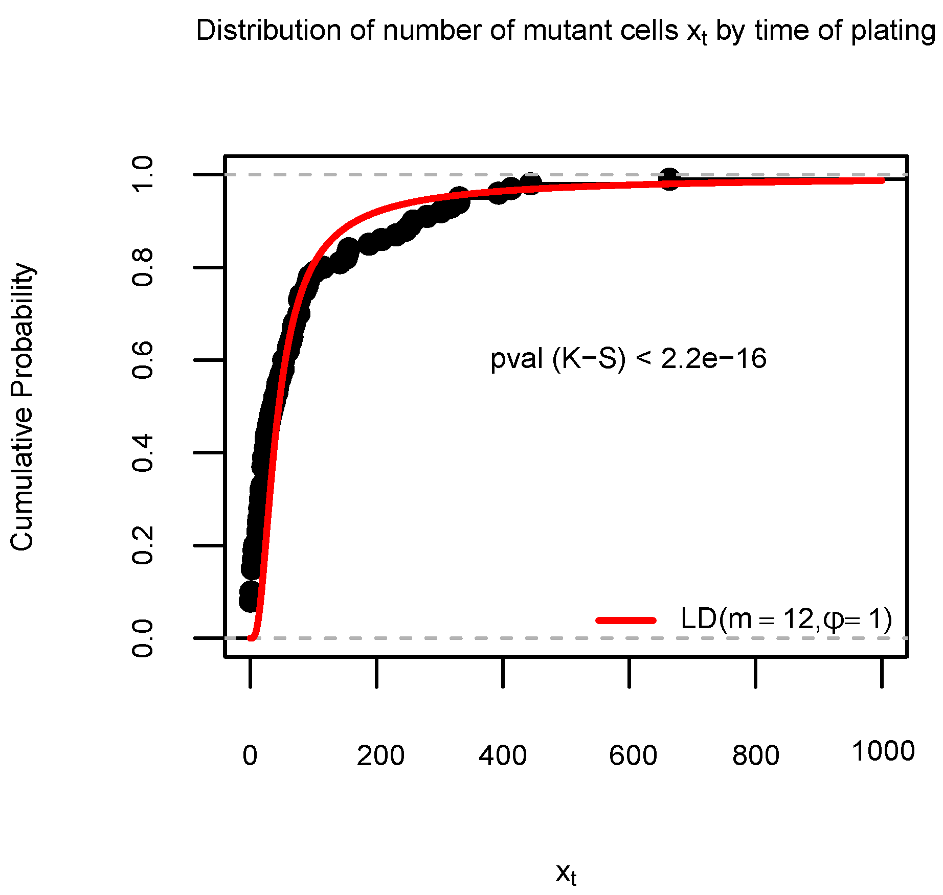
Accordingly, we set for SimuBP the cell lifetime distribution to be $exp\left({\beta }_1\right)$, the time of plating $t_p\approx \frac{1}{{\beta }_1}log{z}_t$, and we approximated the mutation probability $\mu$ by $\frac{\tilde{\mu }}{{\beta }_1}log2$ [19]. Based on 100 simulations, we plotted the ECDF of the resulting $x_t$ samples together with the LD distribution CDF in Figure A1 in Appendix A.2. From Figure A1, it is clear that there exists a remarkable discrepancy between the ECDF of the $x_t$ samples and the LD distribution CDF, due to the difference between the stochastic/deterministic growth assumption for the wild-type cells in the two models.

3.2. Comparison to Alternative Simulators

In Simulation S2a, we used the same settings for SimuBP as in Simulation S1a to generate 100 samples of $z_t$ and $x_t$. Similarly, by using Algorithm 2, another 100 samples of $z_t$ and $x_t$ were generated. We then plotted in Figure 5A the two ECDFs of the $z_t$ samples and plotted in Figure 5B the two ECDFs of the $x_t$ samples, for the data generated from SimuBP (Algorithm 1) and from Algorithm 2. The K-S test p-values were shown beside the curves. Repeating 1000 times, the proportions of significant K-S test p-values are 0.038 (for $z_t$) and 0.053 (for $x_t$), showing that the data generated from these two algorithms are very close in distribution.

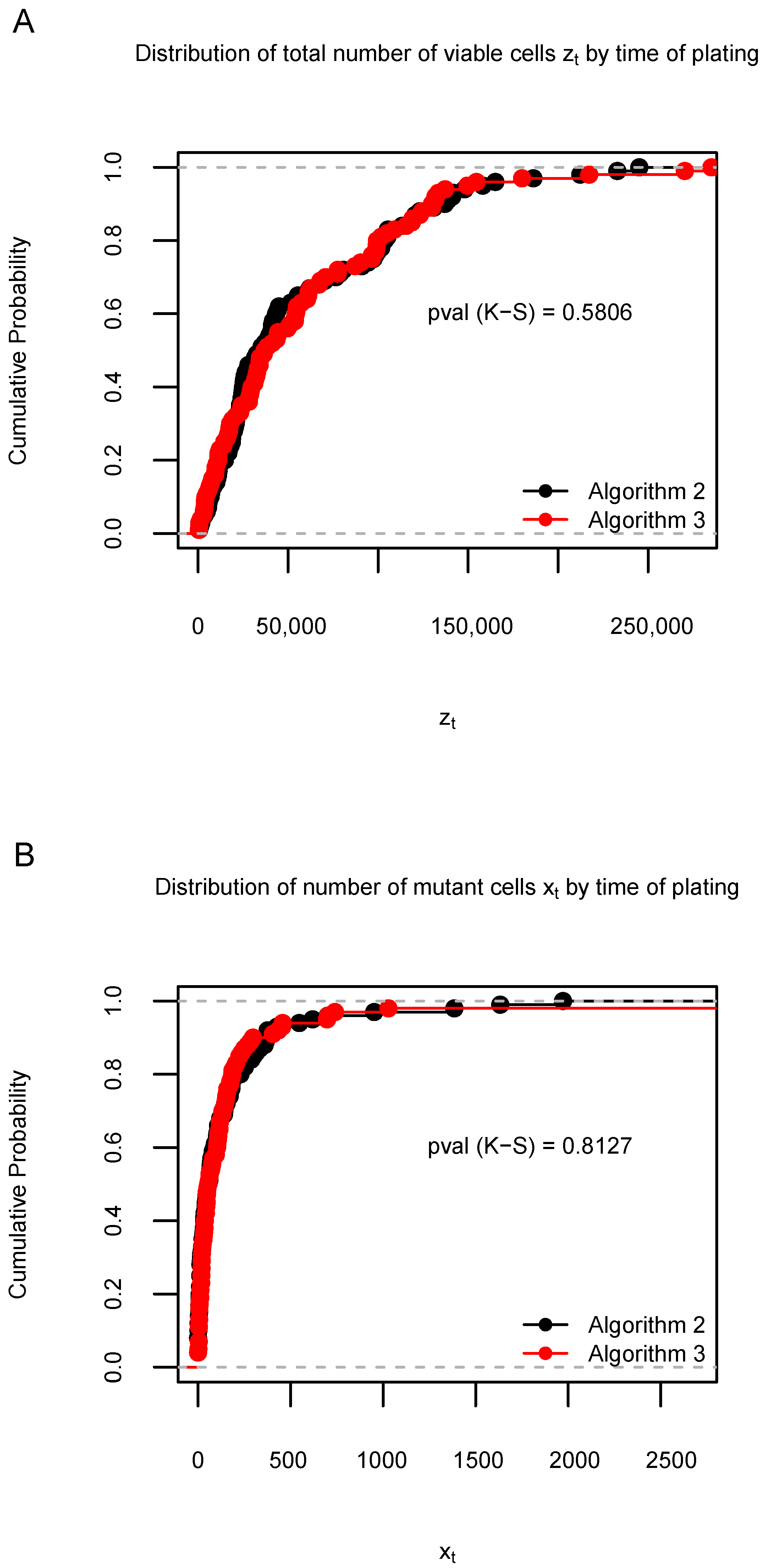
Using the same settings, Simulation S2b compared the distribution of 100 simulated $z_t$ and $x_t$ samples by using Algorithms 1 and 3. This result is shown in Figure 6. The consistency between the data generated from these two algorithms was confirmed by the proportions of significant K-S tests among 1000 repetitions: 0.039 (for $z_t$) and 0.044 (for $x_t$). For completeness, we also included the comparison between the data generated by Algorithms 2 and 3 in Figure A2 in Appendix A.3.

The comparison in computational efficiency of the three algorithms seems not absolutely necessary as we can always improve the simulation speed by increasing the initial number of cells or adjusting the exponential rate of the cell lifetime. Nevertheless, for reference purposes, we provided the average computation time of the three algorithms in

Table 1. Comparison of average computation time (in secs) per sample for simulating 100 data samples *.

Parameters	SimuBP (Algorithm 1)	Algorithm 2	Algorithm 3
${\mu }_1={10}^{-7},t_p=16$	2.7309	4.4873	$2\times {10}^{-4}$
${\mu }_1={10}^{-6},t_p=14$	0.3497	0.5969	$\approx 0$
${\mu }_1={10}^{-5},t_p=12$	0.0523	0.0812	$\approx 0$
${\mu }_1={10}^{-4},t_p=10$	0.0081	0.0111	$\approx 0$
${\mu }_1={10}^{-3},t_p=8$	0.0016	0.0016	$\approx 0$
${\mu }_1={10}^{-2},t_p=6$	0.0005	0.0001	$\approx 0$

* The simulation is based on a simplified two-type branching process (STBP) with initial number of wild-type cells $z_0=1$, exponential rate $a_1=a_2=1$ for wild-type and mutant cell lifetimes, and with mutation probability ${\mu }_1$ and time of plating $t_p$ taking different values.

for simulating data samples with $z_0=1,a_1=a_2=1$ and under different settings of ${\mu }_1$ and $t_p$. It is understandable that as a “exact” simulator of the real cell proliferation and mutation process, SimuBP is not computationally advantageous as compared to other simulators (e.g., Algorithm 3). However, with the aid of high-performance computing facilities, this should not be an issue for the practical use of SimuBP.

3.3. Demonstration of Mutation Rate Estimation Based on Data Generated by SimuBP

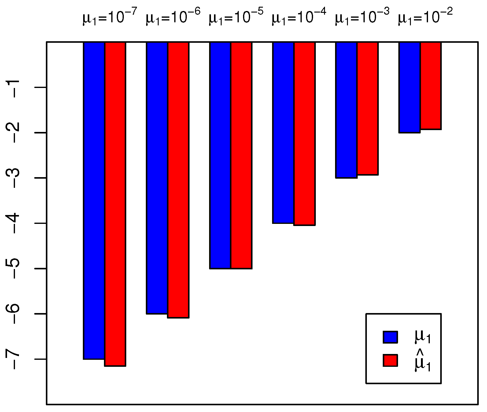
In Simulation S3a, we generated data for $z_t$ and $x_t$ in $J=100$ parallel cultures using SimuBP. The simulated data is based on an STBP with exponential rate 1 and unit initial number of cells (i.e., $y_0=1,x_0=0$). In particular, six different settings on the mutation probability ${\mu }_1$ and the time of plating $t_p$ (both assumed unknown in estimation) were considered, including $({\mu }_1={10}^{-7},t_p=16),({\mu }_1={10}^{-6},t_p=14),\cdots ,({\mu }_1={10}^{-2},t_p=6)$. Based on the simulated data from parallel cultures $(z_{ti},x_{ti}),1\le i\le J$, we estimated ${\mu }_1$ by solving Equation (8) in [12] via the Newton–Raphson method. Repeating the procedure 100 times, we plotted the mean of the estimated ${\mu }_1$ together with its true value in ${log}_{10}$ scale in a barplot in Figure 7, for different values of ${\mu }_1$. The mean squared errors corresponding to ${\mu }_1={10}^{-7}, {10}^{-6}, \cdots , {10}^{-2}$ are: $1.69\times {10}^{-14}, 2.02\times {10}^{-12}, 9.34\times {10}^{-11}, 2.26\times {10}^{-9},$ $2.58\times {10}^{-7}, 6.58\times {10}^{-6}$, respectively.

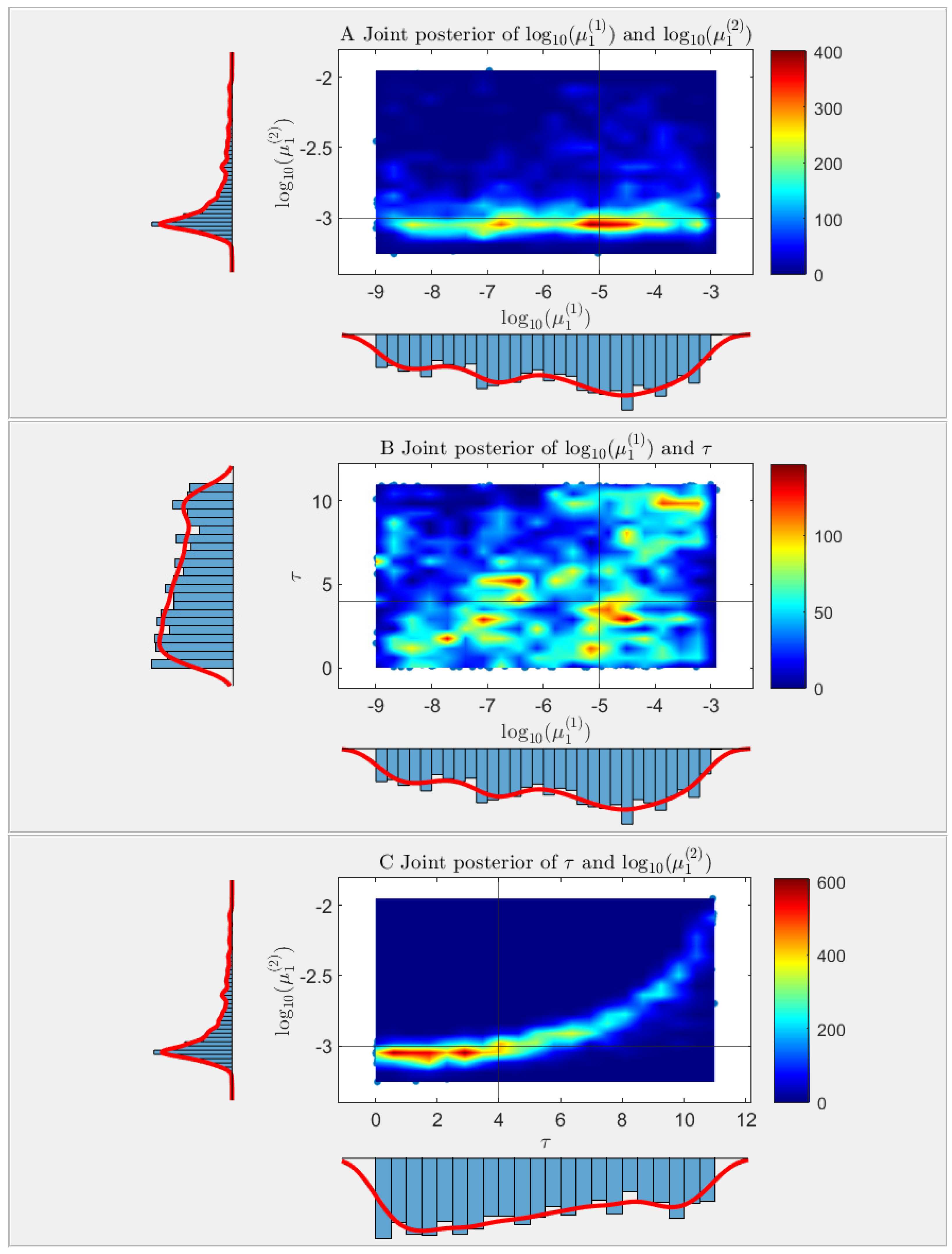
Simulation S3b is based on the same STBP model as in S3a except that the mutation rate parameter (for forward mutation only) is changed to a piece-wise constant function ${\mu }_1\left(t\right)={\mu }_1^{\left(1\right)}{\mathbf{1}}_{0<t\le \tau }+{\mu }_1^{\left(2\right)}{\mathbf{1}}_{\tau <t\le t_p}$, where ${\mu }_1^{\left(1\right)}={10}^{-5},{\mu }_1^{\left(2\right)}={10}^{-3}$ represent the mutation probabilities in the first and second stages, respectively, and $\tau =4$ represents the transition time from stage 1 to stage 2. Denote the unknown parameters by $\Theta ={({\mu }_1^{\left(1\right)},{\mu }_1^{\left(2\right)},\tau )}^T$. Clearly, estimating the three components of $\Theta$ simultaneously would be an impossible task for existing mutation rate estimators. Here we adopted the GPS-ABS approach proposed in [16], which is a likelihood-free, simulation-based estimator via approximate Bayesian computation (ABC) equipped with a Gaussian process surrogate. Briefly speaking, the basic idea of using ABC to estimate parameters without explicit likelihood is “trial and error” through extensive simulations. By repeatedly simulating data and accepting those that are close to the observed data, ABC is able to keep “good” posterior samples of the parameters by using the Metropolis-Hastings algorithm. These posterior samples are then used for inference purposes. In this simulation study, SimuBP was used not only to generate the observed data $(z_t,x_t)$ from the two-stage mutation model but also to train the Gaussian process surrogate to improve the computational efficiency. A total of 50,000 posterior samples of $\Theta$ were collected by applying the GPS-ABC algorithm. Treating the first 35,000 as the burn-in samples of MCMC, we plotted in Figure 8 the heatmap of the joint posterior distribution of each of the two parameters in $\Theta$, with the marginal posterior distributions shown along the axes. Despite the multimodal shape of the posterior distributions (especially for the two parameters ${\mu }_1^{\left(1\right)}$ and $\tau$ as seen in Figure 8B) caused by lack of identifiability of the three model parameters, if we use the highest posterior mode of the joint distribution for posterior inference, the point estimation result is ${\widehat{\mu }}_1^{\left(1\right)}=9.32\times {10}^{-6}, {\widehat{\mu }}_1^{\left(2\right)}=9.59\times {10}^{-4}$ and $\widehat{\tau }=3.75$, close to their true values.

4. Discussion and Conclusions

In this paper, we developed a flexible simulator, called SimuBP, of population dynamics and mutations based on branching processes, and performed simulation studies for validation, comparison, and demonstration purposes. SimuBP is not designed for a particular branching process model, but for a wide range of branching processes, including GWP, MBP, BHP, KTBP, STBP, GTBP, etc. Using the settings of STBP for traditional Luria–Delbrück experiments, the simulation studies showed that SimuBP was able to generate data that (1) follow expected distributions according to STBP, (2) exhibit good consistency with those simulated by two alternative simulators, (3) are applicable for mutation rate estimation. The example of estimating mutation rate in a two-stage mutation process also showed that SimuBP could be incorporated with state-of-the-art ABC methods to enable simulation-based estimation in complex mutation scenarios.

The current version of the SimuBP software is programmed for the GTBP model which involves two distinguishable cells. With some modifications, SimuBP can be extended to model other varieties of branching processes such as the multi-type branching process [7] and the infinite-allele branching process [20,21,22]. These models play important roles in many genetic applications such as metastasis evolution [23] and DNA sequence evolution [24].

Because of its special property of simulating proliferation and mutation “on the basis of each individual cell”, SimuBP can be used to simulate data for more complex models than the traditional Luria–Delbrück or Lea–Coulson models. For better understanding, one may treat the simulation procedure of SimuBP as an in silico fluctuation experiment which is able to take into account realistic experimental conditions, such as non-unit initial number of cells (e.g., unequal or random $z_0$ counts in parallel cultures), multi-fission cell divisions, mutation rate change induced by environmental stimuli, as well as random effects in dilution and plating. Such a simulator will certainly benefit the field of fluctuation analysis by providing real-imitated data or justifying newly-developed theoretical or methodological results in mutation rate estimation.

However, as every coin has two sides, SimuBP also faces computational issues caused by exhaustive simulation. In a typical fluctuation experiment of bacteria, the size of each parallel cell culture may be ${10}^8\sim {10}^{10}$ in a 5-day incubation period before plating. Correspondingly, simulation of such a cell culture by SimuBP usually takes about five seconds on a DELL T5500 computer with XEON quad core X5550, 2.66 GHZ CPU and 24 GB RAM, which is computationally expensive. Such a difficulty may be overcome by borrowing strength from fast-evolving computational resources via parallelism of the SimuBP algorithm on multicore CPUs, GPUs, and computer clusters.

References

- Crump, K.S.; Hoel, D.G. Mathematical models for estimating mutation rates in cell populations. Biometrika 1974, 61, 237–252. [Google Scholar] [CrossRef]
- Harris, T.E. The Theory of Branching Processes; Prentice-Hall: Englewood Cliffs, NJ, USA, 1963. [Google Scholar]
- Galton, F.; Watson, H.W. On the probability of the extinction of families. J. R. Anthropol. Inst. 1875, 4, 138–144. [Google Scholar]
- Bellman, R.; Harris, T.E. On age-dependent binary branching processes. Ann. Math. 1952, 55, 280–295. [Google Scholar] [CrossRef]
- Montgomery-Smith, S.; Oveys, H. Age-dependent branching processes and applications to the Luria–Delbrück experiment. Electron. J. Differ. Equ. 2021, 56, 1–22. [Google Scholar]
- Asmussen, S.; Hering, H. Continuous Time Markov Branching Processes. In Branching Processes. Progress in Probability and Statistics; Birkhäuser: Boston, MA, USA, 1983; Volume 3. [Google Scholar]
- Mode, C.J. Multitype Branching Processes—Theory and Applications; American Elsevier: New York, NY, USA, 1971. [Google Scholar]
- Jagers, P. Branching Processes with Biological Applications; Wiley: Hoboken, NJ, USA, 1975. [Google Scholar]
- Green, P. Modelling yeast cell growth using stochastic branching processes. J. Appl. Probab. 1981, 18, 799–808. [Google Scholar] [CrossRef]
- Kendall, D.G. Birth-and-death processes, and the theory of carcinogenesis. Biometrika 1960, 47, 13–21. [Google Scholar] [CrossRef]
- Cheek, D.; Antal, T. Mutation frequencies in a birth-death branching process. Ann. Appl. Probab. 2018, 28, 3922–3947. [Google Scholar] [CrossRef]
- Wu, X.; Zhu, H. Fast maximum likelihood estimation of mutation rates using a birth–death process. J. Theor. Biol. 2015, 366, 1–7. [Google Scholar] [CrossRef]
- Wu, X.; Zhu, H. Association testing for binary trees—A Markov branching process approach. Stat. Med. 2022, 41, 2557–2573. [Google Scholar] [CrossRef]
- Zheng, Q. Statistical and algorithmic methods for fluctuation analysis with SALVADOR as an implementation. Math. Biosci. 2002, 176, 237–252. [Google Scholar] [CrossRef]
- Thi, T.D.; López, E.; Rodríguez-Rojas, A.; Rodríguez-Beltrán, J.; Couce, A.; Guelfo, J.R.; Castañeda-García, A.; Blázquez, J. Effect of recA inactivation on mutagenesis of Escherichia coli exposed to sublethal concentrations of antimicrobials. J. Antimicrob. Chemother. 2011, 66, 531–538. [Google Scholar] [CrossRef] [PubMed] [Green Version]
- Lu, R.; Zhu, H.; Wu, X. Estimating mutation rates in a Markov branching process using approximate Bayesian computation. J. Theor. Biol. 2023. submitted. [Google Scholar]
- Sarkar, S.; Ma, W.T.; Sandri, G.V. On fluctuation analysis: A new, simple and efficient method for computing the expected number of mutants. Genetica 1992, 85, 173–179. [Google Scholar] [CrossRef] [PubMed]
- Ma, W.T.; Sandri, G.V.; Sarkar, S. Analysis of the Luria-Delbrück distribution using discrete convolution. J. Appl. Probab. 1992, 29, 255–267. [Google Scholar] [CrossRef]
- Zheng, Q. Update on estimation of mutation rates using data from fluctuation experiments. Genetics 2005, 171, 861–864. [Google Scholar] [CrossRef] [PubMed] [Green Version]
- Griffiths, R.C.; Pakes, A.G. An infinite-alleles version of the simple branching process. Adv. Appl. Probab. 1988, 20, 489–524. [Google Scholar] [CrossRef]
- Pakes, A.G. An infinite alleles version of the Markov branching process. J. Aust. Math. Soc. (Ser. A) 1989, 46, 146–170. [Google Scholar] [CrossRef] [Green Version]
- Wu, X.; Kimmel, M. Modeling neutral evolution using an infinite-allele Markov branching process. Int. J. Stoch. Anal. 2013, 2013, 963831. [Google Scholar] [CrossRef] [Green Version]
- Slavtchova-Bojkova, M.; Vitanov, K. Multi-type age-dependent branching processes as models of metastasis evolution. Stoch. Model. 2019, 35, 284–299. [Google Scholar] [CrossRef]
- Kimmel, M.; Mathaes, M. Modeling neutral evolution of Alu elements using a branching process. BMC Genom. 2010, 11 (Suppl. 1), S11. [Google Scholar] [CrossRef] [Green Version]
- Athreya, K.B.; Ney, P.E. Branching Processes; Springer: Berlin/Heidelberg, Germany, 1972. [Google Scholar]
- Kopp-schneider, A. Birth-death processes with piecewise constant rates. Stat. Probab. Lett. 1992, 13, 121–127. [Google Scholar] [CrossRef]
- Renshaw, E. Modeling Biological Populations in Space and Time; Cambridge University Press: Cambridge, UK, 1991. [Google Scholar]
- Karlin, S.; Taylor, H.M. A First Course in Stochastic Processes; Academic Press: Boston, MA, USA, 1975. [Google Scholar]
- Zheng, Q. On a birth-and-death process induced distribution. Biom. J. 1997, 39, 699–705. [Google Scholar] [CrossRef]
Figure 1.
Cell mutations in the KTBP and STBP models.
Figure 2.
Input of the SimuBP algorithm.
Figure 3.
Distribution of 100 data samples generated by SimuBP in Simulation S1a. (A): Empirical cumulative distribution function (ECDF) of the total number of viable cells when the time of plating . (B): ECDF of the number of wild-type cells when . The red curves represent the cumulative distribution function of the theoretical geometric distributions in comparison. The Kolmogorov–Smirnov (K-S) test p-values are shown under the ECDF curves.
Figure 4.
Distribution of 100 data samples generated by SimuBP in Simulation S1b. (A): Empirical cumulative distribution function (ECDF) of the total number of viable cells when the time of plating . (B): ECDF of the number of wild-type cells when . The red curves represent the cumulative distribution function of the theoretical negative binomial distributions in comparison. The Kolmogorov–Smirnov (K-S) test p-values are shown under the ECDF curves.
Figure 5.
Distribution of 100 data samples generated by Algorithms 1 and 2 in Simulation S2a. (A): Empirical cumulative distribution function (ECDF) of the total number of viable cells when the time of plating . (B): ECDF of the number of mutant cells when . The Kolmogorov–Smirnov (K-S) test p-values are shown under the ECDF curves.
Figure 6.
Distribution of 100 data samples generated by Algorithms 1 and 3 in Simulation S2b. (A): Empirical cumulative distribution function (ECDF) of the total number of viable cells when the time of plating . (B): ECDF of the number of mutant cells when . The Kolmogorov–Smirnov (K-S) test p-values are shown under the ECDF curves.
Figure 7.
Estimation of constant mutation probability in Simulation S3a, based on data generated by SimuBP. The blue and red bars represent the true value and the estimated value , respectively. The y-axis is shown in scale.
Figure 8.
Estimation of piece-wise constant mutation probability function in a two-stage mutation model in Simulation S3b, based on data generated by SimuBP. Each panel shows the heatmap of the posterior samples of a pair of the three parameters: first stage mutation probability , second stage mutation probability , and transition time , based on 2-d kernel density estimation. (A): vs. ; (B): vs. ; (C): vs. . The horizontal and vertical black lines mark the true parameter values. The histograms on the left and bottom of each heatmap show the marginal distributions of each two parameters.