A High-Order Approximate Solution for the Nonlinear 3D Volterra Integral Equations with Uniform Accuracy

Abstract

In this paper, we present a high-order approximate solution with uniform accuracy for nonlinear 3D Volterra integral equations. This numerical scheme is constructed based on the three-dimensional block cubic Lagrangian interpolation method. At the same time, we give the local truncation error analysis of the numerical scheme based on Taylor’s theorem. Through theoretical analysis, we reach the conclusion that the optimal convergence order of this high-order numerical scheme is 4. Finally, we verify the effectiveness and applicability of the method through four numerical examples.

1. Introduction

Nonlinear Volterra integral equations (VIEs) are widely used in many practical problems, such as electromagnetism and plasmon progeny physics, hydrodynamics, oscillation theory, polymer rheology, chemical dynamics, biomechanics, and control theory, etc. [1]. However, nonlinear VIEs are equations with nonlinear and integral terms, and only a small part of them can obtain accurate solutions directly. In the process of rapid development in mathematical physics, engineering, medicine, and other fields, more and more researchers have begun to study the numerical calculation methods of nonlinear VIEs [2].

In this paper, we will consider the following nonlinear 3D-VIEs of the form

$$\begin{array}{c}\hfill \mu (x,y,z)=g(x,y,z)+{\int }_0^x{\int }_0^y{\int }_0^{z}K(x,y,z,w,t,\nu ,\mu (w,t,\nu ))d\nu dtdw,\end{array}$$

(1)

where $(x,y,z)\in \Theta$, $g(x,y,z)$ and $K(x,y,z,w,t,\nu ,\mu (w,t,\nu ))$ are given continuous functions defined on $\Theta ={[0,\overline{g}]}^3,\Phi =\Theta \times \Theta \times (-\infty ,+\infty )$, respectively, and $\mu (x,y,z)$ is unknown on $\Theta$.

The rigid-body collisions with friction can be described by a linear VIE considering the impulses and sliding velocities as functions of the direction of the sliding velocity in [3]. The numerical solution for solving the system of VIEs without special starting procedures was given by the block-by-block method (BLBM) in [4]. In [5], the authors give a numerical solution for the second kind of VIE under rigorous error analysis by spectral methods. In [6], the second kind of VIE, with smooth or weakly singular kernels, was solved by the Taylor-series expansion method. In [7], the Laplace transform can be used to solve VIEs by using a new transformation. In [8], the Urysohn-type nonlinear VIEs were solved by the Euler and trapezoidal discretization methods. An ordinary method for constructing the numerical schemes of the fractional ordinary differential equations (FODEs) was introduced by using the idea of BLBM without solving the coupling unknown solutions at each block step in [9]. In [10], they introduced a high-order numerical scheme for FODEs with the Caputo derivative. This numerical scheme is implemented by dividing the interval into a great quantity of subintervals and using quadratic interpolation on them. At the same time, it is shown that the numerical scheme is proved to be unconditionally stable for general nonlinear equations with the uniform sharp convergence order. In [11], the authors propose a high-order numerical scheme for an integro-differential equation with a fractional Caputo derivative based on the shifted Legendre polynomials by coupling the idea of the Gauss–Legendre quadrature rule and spectral collocation method. The second kind of VIE was solved by the Bernstein’s approximation in [12]. Based on the row and column sweep parallel algorithms, a parallel solution of the second kind of linear VIE was given with the suitable quadrature technique in [13]. Some efficient numerical solutions for the linear system of Volterra–Fredholm integral equations (VFIEs) were constructed based on the collocation method with the help of the Bernstein polynomial in [14]. In [15], the numerical solution for the separable kernels VIEs were given by the method of differential transform. By the radial basis functions with scattered points, the VIEs were solved with the analysis of the error estimation and the convergence rate estimation in [16]. In [17], the authors studied the numerical solution of the nonlinear 2D VIE by using the collocation method and iterated collocation method. In [18], the Euler-type numerical solution for the first kind 2D-VIEs was introduced with its convergence analysis. It gave a numerical scheme for solving the 2D differential transform for double integrals in [19]. The numerical solution for 2D nonlinear fractional VFIEs was constructed based on the collocation method by using the block-pulse functions of 2D and the shifted Legendre polynomials of two variables in [20]. In [21], the second 2D nonlinear VIE was solved by the Galerkin method with the help of the moving least squares method. The paper proposed a numerical method to solve 2D-VIEs with fractional order, weakly singular kernels based on 2D Euler polynomials combined with the Gauss–Jacobi quadrature formula in [22]. In [23], an efficient method was presented for solving the second kind of 3D-VFIEs based on 3D Bernstein polynomials. The spectrally accurate collacation method was introduced to solve the second integral equation of a weakly singular kernel by using multivarate Jacobi approximating in [24]. In [25], the results of 2D-VIE was extended to solve 3D-VIE by using the reduced differential transform method. The dimensional differential transform method was applied for solving nonlinear 3D-VIEs in [26]. The authors present an optimal homotopy asymptotic method for solving 3D-VIEs of the second kind in [27]. A new numerical method for solving 3D VFIEs was presented based upon 3D block-pulse functions approximation in [28].

The study of a numerical shceme for nonlinear 3D-VIEs is an essential research topic. Thus far, scholars have limited research on higher-order numerical schemes for nonlinear 3D-VIEs with uniform accuracy, which further strengthens the significance of our research on this topic. In this article, we divide the region into many subdomains and construct a new numerical scheme for nonlinear 3D-VIE by using three-dimensional block cubic Lagrangian interpolation. The scheme has a uniform accuracy and an optimal convergence order of 4. At the same time, we can obtain the convergence analysis of the numerical scheme based on the numerical analysis method, the Granwall inequality and the idea of [18].

The arrangement of the paper is as follows. The existence and uniqueness of the analytical solution is proposed based on the compressed mapping in Section 2. High-order approximate solutions are constructed based on the idea of Lagrangian interpolation methods in Section 3. In Section 4, the local truncation error of the constructed high-order approximate solution is given based on Taylor’s theorem. In Section 5, the convergence analysis of the high-order approximate solution is studied by using the Gronwall inequality. Four numerical examples are given to verify the correctness of convergence theoretical analysis in Section 6. In Section 7, some conclusions are given to discuss the computational efficiency of the high-order approximate solution, and further studies are discussed.

2. Existence and Uniqueness of Solution

For our numerical solution to be meaningful, we will first prove that Equation (1) has a solution and only one solution. Given this condition, a numerical scheme constructed based on Equation (1) makes sense. In this section, to prove this condition, we will establish the existence and uniqueness of the solution in Equation (1) based on the compressive mapping method, and give the corresponding theorem as follows. In this theorem, we define the following symbols: $X=(x,y,z)$ and $W=(w,t,\nu )$ for narrative convenience.

Theorem 1.

Let $K(X,W,\mu )$ satisfy the following condition with respect to variable μ,

$$\begin{array}{c}\hfill |K(X,W,{\mu }_1)-K(X,W,{\mu }_2)|\le L|{\mu }_1-{\mu }_2|,L>0,\end{array}$$

(2)

and then Equation (1) has a unique solution in $\Theta ={[0,\overline{g}]}^3$.

Proof. 

Set ${∥\phi ∥}_{\ast }=\underset{X\in \Theta }{\max }{e}^{-\ell (x+y+z)}{∥\phi (X)∥}_2$, where ${∥·∥}_2$ is the $L^2-$ norm. Suppose S is a continuous space of function on ${[0,\overline{g}]}^3\to R^3$ is defined as $S=\{\psi (X):||\psi (X)|{|}_{\ast }<+\infty ,$$\forall \psi (X),X\in {[0,\overline{g}]}^3\}$. Let $A:S\to S$ be an operator as follows:

$$\begin{array}{c}\hfill A(\phi )(X)=g(X)+{\int }_0^x{\int }_0^y{\int }_0^{z}K(X,W,\phi (W))d\nu dtdw.\end{array}$$

In the following, we will prove that A is a compressed mapping. For $\forall \phi ,\psi \in S$, by a directly calculate we can obtain

$$\begin{array}{cc}\hfill & {\parallel A(\phi )-A(\psi )\parallel }_{\ast }\hfill \\ \hfill =& \underset{X\in \Theta }{max}{e}^{-\ell (x+y+z)}\parallel {\int }_0^x{\int }_0^y{\int }_0^{z}K(X,W,\phi (W))d\nu dtdw-{\int }_0^x{\int }_0^y{\int }_0^{z}K(X,W,\psi (W))d\nu dtdw{\parallel }_2\hfill \\ \hfill \le & \underset{X\in \Theta }{max}{e}^{-\ell (x+y+z)}{\int }_0^x{\int }_0^y{\int }_0^{z}L{e}^{\ell (w+t+\nu )}\left[e^{-\ell (w+t+\nu )}{\parallel \phi (W)-\psi (W)\parallel }_2\right]d\nu dtdw\hfill \\ \hfill \le & \left(\underset{X\in \Theta }{max}{e}^{-\ell (x+y+z)}{\int }_0^x{\int }_0^y{\int }_0^{z}L{e}^{\ell (w+t+\nu )}d\nu dtdw\right){\parallel \phi -\psi \parallel }_{\ast }\hfill \\ \hfill \le & \underset{X\in \Theta }{max}\frac{L(1-e^{-\ell x})(1-e^{-\ell y})(1-e^{-\ell z})}{{\ell }^3}{\parallel \phi -\psi \parallel }_{\ast }\le \frac{L}{{\ell }^3}{\parallel \phi -\psi \parallel }_{\ast }.\hfill \end{array}$$

Choosing $\ell >L^{1/3}>0$, it is easy to show that A is a compressed mapping. Therefore, according to the principle of a compressed fixed point, there is a unique solution $\mu \in S$ that satisfies Equation (1). The proof is then completed. □

3. Construction of the High-Order Approximate Solution

Now we construct the higher-order approximate solution of (1). Let the domain ${[0,\overline{g}]}^3$ be divided into $N^3$ equal subdomains, and set $x_i=y_i=z_i=ih,i=0,1,\cdots ,N$, here $h=\frac{\overline{g}}{N}$. In the following, denoting by ${\mu }_{i,j}^q$ is the numerical solution at point $(x_i,y_j,z_q)$. Meanwhile, according to this definition and formula (1), we have ${\mu }_{i,0}^0=g(x_i,0,0)$, ${\mu }_{0,j}^0=g(0,y_j,0)$, ${\mu }_{0,0}^q=g(0,0,z_q)$, ${\mu }_{i,j}^0=g(x_i,y_j,0)$, ${\mu }_{i,0}^q=g(x_i,0,z_q)$ and ${\mu }_{0,j}^q=g(0,y_j,z_q),$$i,j,q=0,1,\cdots ,N$. For the sake of simplicity, we set $K(x_i,y_j,z_q,w,t,\nu ,\mu (w,t,\nu ))=K_{i,j,q}(w,t,\nu ,\mu (w,t,\nu ))$ and $g(x_i,y_j,z_q)=g_{i,j,q}$ in the following parts.

Let ${\psi }_{i,j}(s),i=0,1,2,3;j\in \mathbb{N}$ be the four basic functions of cubic interpolation at points $s_j,s_{j+1},s_{j+2},s_{j+3}$, respectively, and $s_j=jh$, the definition of ${\psi }_{i,j}(s)$ is

$$\begin{array}{cc}\hfill & {\psi }_{0,j}(s)=\frac{(s-(j+1)h)(s-(j+2)h)(s-(j+3)h)}{-6h^3},\hfill \\ \hfill & {\psi }_{1,j}(s)=\frac{(s-jh)(s-(j+2)h)(s-(j+3)h)}{2h^3},\hfill \\ \hfill & {\psi }_{2,j}(s)=\frac{(s-jh)(s-(j+1)h)(s-(j+3)h)}{-2h^3},\hfill \\ \hfill & {\psi }_{3,j}(s)=\frac{(s-jh)(s-(j+1)h)(s-(j+2)h)}{6h^3}.\hfill \end{array}$$

(3)

First, we construct an approximate solution of $\mu (x_1,y_1,z_1)$, which has

$$\begin{array}{cc}\hfill & \mu (x_1,y_1,z_1)=g_{1,1,1}+{\int }_0^{x_1}{\int }_0^{y_1}{\int }_0^{z_1}{K}_{1,1,1}(w,t,\nu ,\mu (w,t,\nu ))d\nu dtdw\hfill \\ \hfill & \approx g_{1,1,1}+{\int }_0^{x_1}{\int }_0^{y_1}{\int }_0^{z_1}\sum _{a,b,c=0}^3{\psi }_{a,0}(w){\psi }_{b,0}(t){\psi }_{c,0}(\nu )K_{1,1,1}(x_a,y_b,z_c,\mu (x_a,y_b,z_c))d\nu dtdw\hfill \\ \hfill & =g_{1,1,1}+\sum _{a,b,c=0}^3{\lambda }_{a,0}^1{\tilde{\lambda }}_{b,0}^1{\overline{\lambda }}_{c,0}^1{K}_{1,1,1}(x_a,y_b,z_c,\mu (x_a,y_b,z_c)),\hfill \end{array}$$

(4)

where

$${\lambda }_{a,0}^1={\int }_0^{x_1}{\psi }_{a,0}(w)dw,{\tilde{\lambda }}_{b,0}^1={\int }_0^{y_1}{\psi }_{b,0}(t)dt,{\overline{\lambda }}_{c,0}^1={\int }_0^{z_1}{\psi }_{c,0}(\nu )d\nu ,a,b,c=0,1,2,3.$$

Secondly, we compute an approximate solution at point $(x_2,y_1,z_1)$.

$$\begin{array}{cc}\hfill & \mu (x_2,y_1,z_1)=g_{2,1,1}+{\int }_0^{x_2}{\int }_0^{y_1}{\int }_0^{z_1}{K}_{2,1,1}(w,t,\nu ,\mu (w,t,\nu ))d\nu dtdw\hfill \\ \hfill & \approx g_{2,1,1}+{\int }_0^{x_2}{\int }_0^{y_1}{\int }_0^{z_1}\sum _{a,b,c=0}^3{\psi }_{a,0}(w){\psi }_{b,0}(t){\psi }_{c,0}(\nu )K_{2,1,1}(x_a,y_b,z_c,\mu (x_a,y_b,z_c))d\nu dtdw\hfill \\ \hfill & =g_{2,1,1}+\sum _{a,b,c=0}^3{\lambda }_{a,0}^2{\tilde{\lambda }}_{b,0}^1{\overline{\lambda }}_{c,0}^1{K}_{2,1,1}(x_a,y_b,z_c,\mu (x_a,y_b,z_c)),\hfill \end{array}$$

(5)

with

$${\lambda }_{a,0}^2={\int }_0^{x_2}{\psi }_{a,0}(w)dw,a=0,1,2,3.$$

Because the approximate solution can be easily obtained by using the calculation similar to (4) and (5) for the other cases, the calculation process is omitted here. Therefore, the approximate solution for $\mu (x_k,y_l,z_m), k,l,m=1,2,3$ is given as follows:

$$\begin{array}{c}\hfill \mu (x_k,y_l,z_m)\approx g_{k,l,m}+\sum _{a,b,c=0}^3{\lambda }_{a,0}^k{\tilde{\lambda }}_{b,0}^l{\overline{\lambda }}_{c,0}^m{K}_{k,l,m}(x_a,y_b,z_c,\mu (x_a,y_b,z_c)),k,l,m=1,2,3,\end{array}$$

(6)

where

$$\begin{array}{c}\hfill \begin{array}{c}{\displaystyle {\lambda }_{a,0}^k={\int }_0^{x_k}{\psi }_{a,0}(w)dw,{\tilde{\lambda }}_{b,0}^l={\int }_0^{y_l}{\psi }_{b,0}(t)dt,{\overline{\lambda }}_{c,0}^m={\int }_0^{z_m}{\psi }_{c,0}(\nu )d\nu ,}\hfill \\ a,b,c=0,1,2,3;k,l,m=1,2,3.\hfill \end{array}\end{array}$$

(7)

From (6), we can get the high-order numerical scheme for $\mu (x_k,y_l,z_m),k,l,m=1,2,3$ as follows:

$$\begin{array}{c}\hfill {\mu }_{k,l}^m=g_{k,l,m}+\sum _{a,b,c=0}^3{\lambda }_{a,0}^k{\tilde{\lambda }}_{b,0}^l{\overline{\lambda }}_{c,0}^m{K}_{k,l,m}(x_a,y_b,z_c,{\mu }_{a,b}^c),k,l,m=1,2,3.\end{array}$$

(8)

Finally, for $\mu (x_k,y_l,z_m),k,l,m\ge 4$, we can obtain an approximate solution of the form

$$\begin{array}{cc}\hfill & \mu (x_k,y_l,z_m)=g_{k,l,m}+{\int }_0^{x_k}{\int }_0^{y_l}{\int }_0^{z_m}{K}_{k,l,m}(w,t,\nu ,\mu (w,t,\nu ))d\nu dtdw\hfill \\ \hfill =& g_{k,l,m}+{\int }_0^{x_3}{\int }_0^{y_3}{\int }_0^{z_3}{K}_{k,l,m}(w,t,\nu ,\mu (w,t,\nu ))d\nu dtdw\hfill \\ \hfill & +\sum _{d=4}^k\sum _{e=4}^l\sum _{f=4}^m{\int }_{x_{d-1}}^{x_d}{\int }_{y_{e-1}}^{y_e}{\int }_{z_{f-1}}^{z_f}{K}_{k,l,m}(w,t,\nu ,\mu (w,t,\nu ))d\nu dtdw\hfill \\ \hfill \approx & g_{k,l,m}+\sum _{a,b,c=0}^3{\int }_0^{x_3}{\int }_0^{y_3}{\int }_0^{z_3}{\psi }_{a,0}(w){\psi }_{b,0}(t){\psi }_{c,0}(\nu )K_{k,l,m}(x_a,y_b,z_c,\mu (x_a,y_b,z_c))d\nu dtdw\hfill \\ \hfill & +\sum _{d=4}^k\sum _{e=4}^l\sum _{f=4}^m\sum _{a,b,c=0}^3{\int }_{x_{d-1}}^{x_d}{\int }_{y_{e-1}}^{y_e}{\int }_{z_{f-1}}^{z_f}{\psi }_{a,d-3}(w){\psi }_{b,e-3}(t){\psi }_{c,f-3}(\nu )d\nu dtdw\hfill \\ \hfill & \times K_{k,l,m}(x_{d-3+a},y_{e-3+b},z_{f-3+c},\mu (x_{d-3+a},y_{e-3+b},z_{f-3+c}))\hfill \\ \hfill =& g_{k,l,m}+\sum _{a,b,c=0}^3{\lambda }_{a,0}^3{\tilde{\lambda }}_{b,0}^3{\overline{\lambda }}_{c,0}^3{K}_{k,l,m}(x_a,y_b,z_c,\mu (x_a,y_b,z_c))\hfill \\ \hfill & +\sum _{d=4}^k\sum _{e=4}^l\sum _{f=4}^m\sum _{a,b,c=0}^3{\tau }_{a,d-3}^d{\tilde{\tau }}_{b,e-3}^e{\overline{\tau }}_{c,f-3}^f{K}_{k,l,m}(x_{d-3+a},y_{e-3+b},z_{f-3+c},\mu (x_{d-3+a},y_{e-3+b},z_{f-3+c})),\hfill \end{array}$$

(9)

where ${\psi }_{a,0}(w),{\psi }_{a,d-3}(w),{\psi }_{b,0}(t),{\psi }_{b,e-3}(t),{\psi }_{c,0}(\nu ),{\psi }_{c,f-3}(\nu )$, and ${\lambda }_{a,0}^3,{\tilde{\lambda }}_{b,0}^3,{\overline{\lambda }}_{c,0}^3$ are defined in (3) and (7), respectively, and

$$\begin{array}{cc}\hfill & {\tau }_{a,d-3}^d={\int }_{x_{d-1}}^{x_d}{\psi }_{a,d-3}(w)dw,a=0,1,2,3;d=4,5,\cdots ,k,\hfill \\ \hfill & {\tilde{\tau }}_{b,e-3}^e={\int }_{y_{e-1}}^{y_e}{\psi }_{b,e-3}(t)dt,b=0,1,2,3;e=4,5,\cdots ,l,\hfill \\ \hfill & {\overline{\tau }}_{c,f-3}^f={\int }_{z_{f-1}}^{z_f}{\psi }_{c,f-3}(\nu )d\nu ,c=0,1,2,3;f=4,5,\cdots ,m.\hfill \end{array}$$

According to the estimated formula of (9), we can easily obtain the numerical scheme at point $(x_k,y_l,z_m),k,l,m=4,5,\cdots ,N$ as follows:

$$\begin{array}{cc}\hfill & {\mu }_{k,l}^m=g_{k,l,m}+\sum _{a,b,c=0}^3{\lambda }_{a,0}^3{\tilde{\lambda }}_{b,0}^3{\overline{\lambda }}_{c,0}^3{K}_{k,l,m}(x_a,y_b,z_c,{\mu }_{a,b}^c)\hfill \\ \hfill & +\sum _{d=4}^k\sum _{e=4}^l\sum _{f=4}^m\sum _{a,b,c=0}^3{\tau }_{a,d-3}^d{\tilde{\tau }}_{b,e-3}^e{\overline{\tau }}_{c,f-3}^f{K}_{k,l,m}(x_{d-3+a},y_{e-3+b},z_{f-3+c},{\mu }_{d-3+a,e-3+b}^{f-3+c}).\hfill \end{array}$$

(10)

To summarize, by combining (8) and (10), we can get the higher-order numerical scheme of problem (1) as follows:

$$\begin{array}{c}\hfill \left\{\begin{array}{cc}& {\mu }_{k,l}^m=g_{k,l,m}+\sum _{a,b,c=0}^3{\lambda }_{a,0}^k{\tilde{\lambda }}_{b,0}^l{\overline{\lambda }}_{c,0}^m{K}_{k,l,m}(x_a,y_b,z_c,{\mu }_{a,b}^c),k,l,m=1,2,3.\hfill \\ & {\mu }_{k,l}^m=g_{k,l,m}+\sum _{a,b,c=0}^3{\lambda }_{a,0}^3{\tilde{\lambda }}_{b,0}^3{\overline{\lambda }}_{c,0}^3{K}_{k,l,m}(x_a,y_b,z_c,{\mu }_{a,b}^c)\hfill \\ & +\sum _{d=4}^k\sum _{e=4}^l\sum _{f=4}^m\sum _{a,b,c=0}^3{\tau }_{a,d-3}^d{\tilde{\tau }}_{b,e-3}^e{\overline{\tau }}_{c,f-3}^f{K}_{k,l,m}(x_{d-3+a},y_{e-3+b},z_{f-3+c},{\mu }_{d-3+a,e-3+b}^{f-3+c}),\hfill \\ & k,l,m=4,5,\cdots ,N.\hfill \end{array}\right.\end{array}$$

(11)

4. Estimation of the Truncation Error

This section mainly deals with the truncation error analysis of the numerical scheme (11) of problem (1). Here we give the following definition:

$$\begin{array}{c}\hfill E_{k,l,m}\doteq \mu (x_k,y_l,z_m)-\overline{\mu }(x_k,y_l,z_m),\end{array}$$

(12)

where $E_{k,l,m}$ represents the truncation error at point $(x_k,y_l,z_m)$ produced by the numerical scheme proposed in Section 3, $\mu (x_k,y_l,z_m)$ is the exact solution of problem (1) in this paper at point $(x_k,y_l,z_m)$, and $\overline{\mu }(x_k,y_l,z_m)$ is an approximate value. We replace the numerical solution ${\mu }_{k,l}^m$ on the right side of Equation (11) with the value obtained after the corresponding exact solution $\mu (x_k,y_l,z_m)$, which is expressed as $\overline{\mu }(x_k,y_l,z_m)$; for example,

$$\begin{array}{c}\hfill \left\{\begin{array}{cc}& \overline{\mu }(x_k,y_l,z_m)=g_{k,l,m}+\sum _{a,b,c=0}^3{\lambda }_{a,0}^k{\tilde{\lambda }}_{b,0}^l{\overline{\lambda }}_{c,0}^m{K}_{k,l,m}(x_a,y_b,z_c,\mu (x_a,y_b,z_c)),k,l,m=1,2,3.\hfill \\ & \overline{\mu }(x_k,y_l,z_m)=g_{k,l,m}+\sum _{a,b,c=0}^3{\lambda }_{a,0}^3{\tilde{\lambda }}_{b,0}^3{\overline{\lambda }}_{c,0}^3{K}_{k,l,m}(x_a,y_b,z_c,\mu (x_a,y_b,z_c))\hfill \\ & +\sum _{d=4}^k\sum _{e=4}^l\sum _{f=4}^m\sum _{a,b,c=0}^3{\tau }_{a,d-3}^d{\tilde{\tau }}_{b,e-3}^e{\overline{\tau }}_{c,f-3}^f{K}_{k,l,m}(x_{d-3+a},y_{e-3+b},z_{f-3+c},\mu (x_{d-3+a},y_{e-3+b},z_{f-3+c})),\hfill \\ & k,l,m=4,5,\cdots ,N.\hfill \end{array}\right.\end{array}$$

(13)

Based on Taylor’s theorem, we will introduce the following lemma to estimate the truncation error of the numerical scheme (11) proposed in Section 3. For the convenience of description, we set $\frac{{\partial }^{4}K}{\partial s^4}={\partial }_s^{4}K$.

Lemma 1.

Suppose the function $K\in C^4({[0,\overline{g}]}^3)$, and $E_{k,l,m}$ represents the truncation error defined in (12), and then it holds that

$$\begin{array}{c}\hfill |E_{k,l,m}|\le C{h}^4,k,l,m=1,2,\cdots ,N,\end{array}$$

(14)

where C is a positive constant that only depends on $\overline{g},M$, with

$$\begin{array}{c}\hfill \begin{array}{ccc}M\hfill & =\hfill & \underset{{[0,\overline{g}]}^3}{max}(|{\partial }_w^{4}K(x,y,z,w,t,\nu ,\mu (w,t,\nu ))|,|{\partial }_t^{4}K(x,y,z,w,t,\nu ,\mu (w,t,\nu ))|,\hfill \\ & & |{\partial }_{\nu }^{4}K(x,y,z,w,t,\nu ,\mu (w,t,\nu ))|).\hfill \end{array}\end{array}$$

(15)

Proof. 

We first estimate $E_{k,l,m},k,l,m=1,2,3$ and according to the definition of truncation error, we bring (1) and (13) into (12) to obtain

$$\begin{array}{cc}\hfill & E_{k,l,m}={\int }_0^{x_k}{\int }_0^{y_l}{\int }_0^{z_m}{K}_{k,l,m}(w,t,\nu ,\mu (w,t,\nu ))d\nu dtdw\hfill \\ \hfill & -{\int }_0^{x_k}{\int }_0^{y_l}{\int }_0^{z_m}\sum _{a,b,c=0}^3{\psi }_{a,0}(w){\psi }_{b,0}(t){\psi }_{c,0}(\nu )K_{k,l,m}(x_a,y_b,z_c,\mu (x_a,y_b,z_c))d\nu dtdw\hfill \\ \hfill =& {\int }_0^{x_k}{\int }_0^{y_l}{\int }_0^{z_m}(K_{k,l,m}(w,t,\nu ,\mu (w,t,\nu ))\hfill \\ \hfill & -\sum _{a,b,c=0}^3{\psi }_{a,0}(w){\psi }_{b,0}(t){\psi }_{c,0}(\nu )K_{k,l,m}(x_a,y_b,z_c,\mu (x_a,y_b,z_c)))d\nu dtdw\hfill \\ \hfill \doteq & {\int }_0^{x_k}{\int }_0^{y_l}{\int }_0^{z_m}{\gamma }_{1}d\nu dtdw.\hfill \end{array}$$

(16)

According to Taylor’s theorem, we can know that for all $(w,t,\nu )\in [0,x_k]\times [0,y_l]\times [0,z_m],k,l,m=1,2,3$, there exists $({\xi }_k(w),{\vartheta }_l(t),{\varrho }_m(\nu ))\in [0,x_k]\times [0,y_l]\times [0,z_m]$, which satisfies

$$\begin{array}{cc}\hfill {\gamma }_1=& \frac{1}{4!}{\partial }_w^4{K}_{k,l,m}({\xi }_k(w),t,\nu ,\mu ({\xi }_k(w),t,\nu ))\prod _{a=0}^3(w-x_a)\hfill \\ \hfill & +\sum _{a=0}^3{\psi }_{a,0}(w)\frac{1}{4!}{\partial }_t^4{K}_{k,l,m}(x_a,{\vartheta }_l(t),\nu ,\mu (x_a,{\vartheta }_l(t),\nu ))\prod _{b=0}^3(t-y_b)\hfill \\ \hfill & +\sum _{a=0}^3\sum _{b=0}^3{\psi }_{a,0}(w){\psi }_{b,0}(t)\frac{1}{4!}{\partial }_{\nu }^4{K}_{k,l,m}(x_a,y_b,{\varrho }_m(\nu ),\mu (x_a,y_b,{\varrho }_m(\nu )))\prod _{c=0}^3(\nu -z_c).\hfill \end{array}$$

(17)

Through the definition of the interpolation basis functions ${\psi }_{a,0}(w),{\psi }_{b,0}(t)$, with $w\in (0,x_k),t\in (0,y_l)$, $a,b=0,1,2,3;k,l=1,2,3$, we can know that $|{\psi }_{a,0}(w)|\le 1$, $|{\psi }_{b,0}(t)|\le 1$. Therefore, we can get the conclusion that $|{\displaystyle \sum _{a=0}^3}{\psi }_{a,0}(w)|\le 4$ and $|{\displaystyle \sum _{a=0}^3}{\displaystyle \sum _{b=0}^3}{\psi }_{a,0}(w){\psi }_{b,0}(t)|\le 16$.

Combining (16) and (17) for $k,l,m=1$, we directly get

$$\begin{array}{cc}\hfill & |E_{1,1,1}|\le |{\int }_0^{x_1}{\int }_0^{y_1}{\int }_0^{z_1}\frac{1}{4!}{\partial }_w^4{K}_{1,1,1}({\xi }_1(w),t,\nu ,\mu ({\xi }_1(w),t,\nu ))\prod _{a=0}^3(w-x_a)d\nu dtdw|\hfill \\ \hfill & +|{\int }_0^{x_1}{\int }_0^{y_1}{\int }_0^{z_1}\sum _{a=0}^3{\psi }_{a,0}(w)\frac{1}{4!}{\partial }_t^4{K}_{1,1,1}(x_a,{\vartheta }_1(t),\nu ,\mu (x_a,{\vartheta }_1(t),\nu ))\prod _{b=0}^3(t-y_b)d\nu dtdw|\hfill \\ \hfill & +|{\int }_0^{x_1}{\int }_0^{y_1}{\int }_0^{z_1}\sum _{a=0}^3\sum _{b=0}^3{\psi }_{a,0}(w){\psi }_{b,0}(t)\frac{1}{4!}{\partial }_{\nu }^4{K}_{1,1,1}(x_a,y_b,{\varrho }_1(\nu ),\mu (x_a,y_b,{\varrho }_1(\nu )))\prod _{c=0}^3(\nu -z_c)d\nu dtdw|\hfill \\ \hfill & \doteq {\gamma }_1^1+{\gamma }_1^2+{\gamma }_1^3.\hfill \end{array}$$

(18)

Now, we analyze the terms on the right side of Equation (18) one by one, and we get

$$\begin{array}{cc}\hfill {\gamma }_1^1& \le {\int }_0^{x_1}{\int }_0^{y_1}{\int }_0^{z_1}\frac{1}{4!}M\times |\prod _{a=0}^3(w-x_a)|d\nu dtdw\hfill \end{array}$$

$$\begin{array}{cc}\hfill & \le M{h}^4{\int }_0^{x_1}{\int }_0^{y_1}{\int }_0^{z_1}1d\nu dtdw=M{h}^7,\hfill \end{array}$$

(19)

$$\begin{array}{cc}\hfill {\gamma }_1^2& \le \frac{4}{4!}M{h}^4{\int }_0^{x_1}{\int }_0^{y_1}{\int }_0^{z_1}1d\nu dtdw\le M{h}^7,\hfill \end{array}$$

(20)

$$\begin{array}{cc}\hfill {\gamma }_1^3& \le \frac{16}{4!}M{h}^4{\int }_0^{x_1}{\int }_0^{y_1}{\int }_0^{z_1}1d\nu dtdw\le M{h}^7,\hfill \end{array}$$

(21)

where M is defined in (15).

Through (18)–(21), we can directly get the conclusion of

$$\begin{array}{c}\hfill |E_{1,1,1}|\le 3M{h}^7.\end{array}$$

By using the same method, we can estimate the error as

$$\begin{array}{c}\hfill |E_{k,l,m}|\le 3M{h}^7,k,l,m=1,2,3.\end{array}$$

(22)

Next, we will analyze the case of $k,l,m\ge 4$, combining (1), (12), and (13), we have

$$\begin{array}{cc}\hfill & |E_{k,l,m}|=|{\int }_0^{x_k}{\int }_0^{y_l}{\int }_0^{z_m}{K}_{k,l,m}(w,t,\nu ,\mu (w,t,\nu ))d\nu dtdw-\sum _{a,b,c=0}^3{\lambda }_{a,0}^3{\tilde{\lambda }}_{b,0}^3{\overline{\lambda }}_{c,0}^3{K}_{k,l,m}(x_a,y_b,z_c,\mu (x_a,y_b,z_c))\hfill \\ \hfill & -\sum _{d=4}^k\sum _{e=4}^l\sum _{f=4}^m\sum _{a,b,c=0}^3{\tau }_{a,d-3}^d{\tilde{\tau }}_{b,e-3}^e{\overline{\tau }}_{c,f-3}^f{K}_{k,l,m}(x_{d-3+a},y_{e-3+b},z_{f-3+c},\mu (x_{d-3+a},y_{e-3+b},z_{f-3+c}))|\hfill \\ \hfill & \le |{\int }_0^{x_3}{\int }_0^{y_3}{\int }_0^{z_3}(K_{k,l,m}(w,t,\nu ,\mu (w,t,\nu ))\hfill \\ \hfill & -\sum _{a,b,c=0}^3{\psi }_{a,0}(w){\psi }_{b,0}(t){\psi }_{c,0}(\nu )K_{k,l,m}(x_a,y_b,z_c,\mu (x_a,y_b,z_c)))d\nu dtdw|\hfill \\ \hfill & +|\sum _{d=4}^k\sum _{e=4}^l\sum _{f=4}^m{\int }_{x_{d-1}}^{x_d}{\int }_{y_{e-1}}^{y_e}{\int }_{z_{f-1}}^{z_f}(K_{k,l,m}(w,t,\nu ,\mu (w,t,\nu ))\hfill \\ \hfill & -\sum _{a,b,c=0}^3{\psi }_{a,d-3}(w){\psi }_{b,e-3}(t){\psi }_{c,f-3}(\nu )K_{k,l,m}(x_{d-3+a},y_{e-3+b},z_{f-3+c},\mu (x_{d-3+a},y_{e-3+b},z_{f-3+c}))d\nu dtdw|\hfill \\ \hfill & \doteq |{\int }_0^{x_3}{\int }_0^{y_3}{\int }_0^{z_3}{\gamma }_{2}d\nu dtdw|+|\sum _{d=4}^k\sum _{e=4}^l\sum _{f=4}^m{\int }_{x_{d-1}}^{x_d}{\int }_{y_{e-1}}^{y_e}{\int }_{z_{f-1}}^{z_f}{\gamma }_{3}d\nu dtdw|.\hfill \end{array}$$

(23)

First, we analyze the first term on the right side of (23). Similar to the estimation of (18), we have

$$\begin{array}{c}\hfill |{\int }_0^{x_3}{\int }_0^{y_3}{\int }_0^{z_3}{\gamma }_{2}d\nu dtdw|\le 3M{h}^7.\end{array}$$

(24)

Next, we estimate the second term on the right side of (23), and for all $(w,t,\nu )\in [x_{d-1},x_d]\times [y_{e-1},y_e]\times [z_{f-1},z_f]$, there are $({\xi }_d(w),{\vartheta }_e(t),{\varrho }_f(\nu ))\in [x_{d-1},x_d]\times [y_{e-1},y_e]\times [z_{f-1},z_f]$, which satisfies

$$\begin{array}{cc}\hfill & {\gamma }_3=\frac{1}{4!}{\partial }_w^4{K}_{k,l,m}({\xi }_d(w),t,\nu ,\mu ({\xi }_d(w),t,\nu ))\prod _{a=0}^3(w-x_{d-3+a})\hfill \\ \hfill & +\sum _{a=0}^3{\psi }_{a,d-3}(w)\frac{1}{4!}{\partial }_t^4{K}_{k,l,m}(x_{d-3+a},{\vartheta }_e(t),\nu ,\mu (x_{d-3+a},{\vartheta }_e(t),\nu ))\prod _{b=0}^3(t-y_{e-3+b})\hfill \\ \hfill & +\sum _{a=0}^3\sum _{b=0}^3{\psi }_{a,d-3}(w){\psi }_{b,e-3}(t)\frac{1}{4!}{\partial }_{\nu }^4{K}_{k,l,m}(x_{d-3+a},y_{e-3+b},{\varrho }_f(\nu ),\mu (x_{d-3+a},y_{e-3+b},{\varrho }_f(\nu )))\prod _{c=0}^3(\nu -z_{f-3+c}).\hfill \end{array}$$

(25)

Therefore, we obtain that

$$\begin{array}{cc}\hfill & |\sum _{d=4}^k\sum _{e=4}^l\sum _{f=4}^m{\int }_{x_{d-1}}^{x_d}{\int }_{y_{e-1}}^{y_e}{\int }_{z_{f-1}}^{z_f}{\gamma }_{3}d\nu dtdw|\hfill \\ \hfill \le & |\sum _{d=4}^k\sum _{e=4}^l\sum _{f=4}^m{\int }_{x_{d-1}}^{x_d}{\int }_{y_{e-1}}^{y_e}{\int }_{z_{f-1}}^{z_f}\frac{1}{4!}{\partial }_w^4{K}_{k,l,m}({\xi }_d(w),t,\nu ,\mu ({\xi }_d(w),t,\nu ))\prod _{a=0}^3(w-x_{d-3+a})d\nu dtdw|\hfill \\ \hfill & +|\sum _{d=4}^k\sum _{e=4}^l\sum _{f=4}^m{\int }_{x_{d-1}}^{x_d}{\int }_{y_{e-1}}^{y_e}{\int }_{z_{f-1}}^{z_f}\sum _{a=0}^3{\psi }_{a,d-3}(w)\frac{1}{4!}{\partial }_t^4{K}_{k,l,m}(x_{d-3+a},{\vartheta }_e(t),\nu ,\mu (x_{d-3+a},{\vartheta }_e(t),\nu ))\hfill \\ \hfill & \times \prod _{b=0}^3(t-y_{e-3+b})d\nu dtdw|+|\sum _{d=4}^k\sum _{e=4}^l\sum _{f=4}^m{\int }_{x_{d-1}}^{x_d}{\int }_{y_{e-1}}^{y_e}{\int }_{z_{f-1}}^{z_f}\sum _{a=0}^3\sum _{b=0}^3{\psi }_{a,d-3}(w){\psi }_{b,e-3}(t)\hfill \\ \hfill & \times \frac{1}{4!}{\partial }_{\nu }^4{K}_{k,l,m}(x_{d-3+a},y_{e-3+b},{\varrho }_f(\nu ),\mu (x_{d-3+a},y_{e-3+b},{\varrho }_f(\nu )))\times \prod _{c=0}^3(\nu -z_{f-3+c})d\nu dtdw|\hfill \\ \hfill & \doteq {\gamma }_3^1+{\gamma }_3^2+{\gamma }_3^3.\hfill \end{array}$$

(26)

Next, we analyze each item in (26) one by one, and we have

$$\begin{array}{cc}\hfill {\gamma }_3^1& \le M{h}^4\sum _{d=4}^k\sum _{e=4}^l\sum _{f=4}^m{\int }_{x_{d-1}}^{x_d}{\int }_{y_{e-1}}^{y_e}{\int }_{z_{f-1}}^{z_f}1d\nu dtdw\hfill \end{array}$$

$$\begin{array}{cc}\hfill & =M{h}^4{\int }_{x_3}^{x_k}{\int }_{y_3}^{y_l}{\int }_{z_3}^{z_m}1d\nu dtdw\le {\overline{g}}^{3}M{h}^4,\hfill \end{array}$$

(27)

$$\begin{array}{cc}\hfill {\gamma }_3^2& \le M{h}^4\sum _{d=4}^k\sum _{e=4}^l\sum _{f=4}^m{\int }_{x_{d-1}}^{x_d}{\int }_{y_{e-1}}^{y_e}{\int }_{z_{f-1}}^{z_f}1d\nu dtdw\le {\overline{g}}^{3}M{h}^4,\hfill \end{array}$$

(28)

$$\begin{array}{cc}\hfill {\gamma }_3^3& \le M{h}^4\sum _{d=4}^k\sum _{e=4}^l\sum _{f=4}^m{\int }_{x_{d-1}}^{x_d}{\int }_{y_{e-1}}^{y_e}{\int }_{z_{f-1}}^{z_f}1d\nu dtdw\le {\overline{g}}^{3}M{h}^4.\hfill \end{array}$$

(29)

Consequently, combining (23), (24) and (26)–(29), we can get the following result

$$\begin{array}{c}\hfill |E_{k,l,m}|\le 3M{h}^7+3{\overline{g}}^{3}M{h}^4,k,l,m=4,5,\cdots ,N.\end{array}$$

(30)

From the conclusions of above (22) and (30), we can obtain the truncation error of the proposed higher-order numerical scheme (11) as follows:

$$\begin{array}{c}\hfill |E_{k,l,m}|\le C{h}^4,k,l,m=1,2,\cdots ,N,\end{array}$$

(31)

where C is a positive constant that only depends on $\overline{g},M$. □

5. Convergence Analysis

For the coefficients appearing in the higher-order numerical scheme (11) proposed in Section 3, we can get the following conclusions through accurate calculation.

$$\begin{array}{cc}\hfill & |{\lambda }_{a,0}^j|\le Ch,|{\tilde{\lambda }}_{a,0}^j|\le Ch,|{\overline{\lambda }}_{a,0}^j|\le Ch,a=0,1,2,3;j=1,2,3,\hfill \end{array}$$

(32)

$$\begin{array}{cc}\hfill & |{\tau }_{a,j-3}^j|\le Ch,|{\tilde{\tau }}_{a,j-3}^j|\le Ch,|{\overline{\tau }}_{a,j-3}^j|\le Ch,a=0,1,2,3;j=4,5,\cdots ,N,\hfill \end{array}$$

(33)

where C is a constant independent of h.

Theorem 2.

Let the function $K\in C^4({[0,\overline{g}]}^3)$ satisfy (2). Let $\mu (x_k,y_l,z_m)$ and ${\mu }_{k,l}^m$ be the solutions of (1) and (11) at points $(x_k,y_l,z_m)$, respectively. If h is small enough, then

$$\begin{array}{c}\hfill |\mu (x_k,y_l,z_m)-{\mu }_{k,l}^m|\le C{h}^4,k,l,m=1,2,\cdots ,N,\end{array}$$

(34)

where C is independent of h.

Proof. 

We first define the error, let ${\epsilon }_{k,l,m}=\mu (x_k,y_l,z_m)-{\mu }_{k,l}^m,k,l,m=0,1,\cdots ,N$. Combining the definitions of ${\epsilon }_{k,l,m}$ and Equation (1), we can easily get

$$\begin{array}{c}\hfill {\epsilon }_{k,0,0}={\epsilon }_{0,l,0}={\epsilon }_{0,0,m}={\epsilon }_{k,l,0}={\epsilon }_{k,0,m}={\epsilon }_{0,l,m}=0,k,l,m=0,1,\cdots ,N.\end{array}$$

(35)

Now, we begin to analyze ${\epsilon }_{k,l,m},k,l,m=1,2,3$, and ${\epsilon }_{k,l,m}$ satisfies

$$\begin{array}{ccc}\hfill {\epsilon }_{k,l,m}& =& \mu (x_k,y_l,z_m)-{\mu }_{k,l}^m=\mu (x_k,y_l,z_m)-\overline{\mu }(x_k,y_l,z_m)+\overline{\mu }(x_k,y_l,z_m)-{\mu }_{k,l}^m\hfill \\ & =& E_{k,l,m}+\overline{\mu }(x_k,y_l,z_m)-{\mu }_{k,l}^m.\hfill \end{array}$$

According to (11), (13), Lemma 1 and (32), we have

$$\begin{array}{cc}\hfill |{\epsilon }_{k,l,m}|& \le |E_{k,l,m}|+|C{h}^3\sum _{a,b,c=0}^3[K_{k,l,m}(x_a,y_b,z_c,\mu (x_a,y_b,z_c))-K_{k,l,m}(x_a,y_b,z_c,{\mu }_{a,b}^c)]|\hfill \\ \hfill & \le C{h}^4+CL{h}^3\sum _{a,b,c=0}^3|\mu (x_a,y_b,z_c)-{\mu }_{a,b}^c|\hfill \\ \hfill & =C{h}^4+CL{h}^3\sum _{a,b,c=0}^3|{\epsilon }_{a,b,c}|,k,l,m=1,2,3.\hfill \end{array}$$

(36)

Simultaneously with the inequality in (36), we easily get

$$|{\epsilon }_{k,l,m}|\le C{h}^4,k,l,m=1,2,3.$$

(37)

Next, we analyze ${\epsilon }_{k,l,m},k,l,m=4,5,\cdots ,N$. According to the definition of ${\epsilon }_{k,l,m}$, combined with (32), (33), and Lemma 1, we can obtain

$$\begin{array}{cc}\hfill |{\epsilon }_{k,l,m}|& \le |C{h}^3\sum _{a=0}^k\sum _{b=0}^l\sum _{c=0}^m(K_{k,l,m}(x_a,y_b,z_c,\mu (x_a,y_b,z_c))-K_{k,l,m}(x_a,y_b,z_c,{\mu }_{a,b}^c))|+|E_{k,l,m}|\hfill \\ \hfill & \le CL{h}^3\sum _{a=0}^k\sum _{b=0}^l\sum _{c=0}^m|{\epsilon }_{a,b,c}|+C{h}^4,k,l,m=4,5,\cdots ,N.\hfill \end{array}$$

(38)

At the same time, we can get

$$\begin{array}{cc}\hfill |{\epsilon }_{k,l,m}|\le & CL{h}^3(\sum _{a=0}^{k-1}\sum _{b=0}^{l-1}\sum _{c=0}^{m-1}|{\epsilon }_{a,b,c}|+\sum _{b=0}^{l-1}\sum _{c=0}^{m-1}|{\epsilon }_{k,b,c}|+\sum _{a=0}^{k-1}\sum _{c=0}^{m-1}|{\epsilon }_{a,l,c}|+\sum _{a=0}^{k-1}\sum _{b=0}^{l-1}|{\epsilon }_{a,b,m}|\hfill \\ \hfill & +\sum _{c=0}^{m-1}|{\epsilon }_{k,l,c}|+\sum _{b=0}^{l-1}|{\epsilon }_{k,b,m}|+\sum _{a=0}^{k-1}|{\epsilon }_{a,l,m}|+|{\epsilon }_{k,l,m}|)+C{h}^4.\hfill \end{array}$$

(39)

Take $||{\widehat{\epsilon }}_{a,b}||=\underset{0\le c\le N}{max}|{\epsilon }_{a,b,c}|$, $a=0,1,\cdots ,k;b=0,1,2\cdots ,l;c=0,1,\cdots ,m$. Then the above inequality can be equivalent to

$$\begin{array}{cc}\hfill & (1-CL\overline{g}{h}^2-CL{h}^3)||{\widehat{\epsilon }}_{k,l}||\hfill \\ \hfill \le & (CL\overline{g}{h}^2+CL{h}^3)\sum _{a=0}^{k-1}\sum _{b=0}^{l-1}||{\widehat{\epsilon }}_{a,b}||+(CL\overline{g}{h}^2+CL{h}^3)\sum _{b=0}^{l-1}||{\widehat{\epsilon }}_{k,b}||\hfill \\ \hfill & +(CL\overline{g}{h}^2+CL{h}^3)\sum _{a=0}^{k-1}||{\widehat{\epsilon }}_{a,l}||+C{h}^4.\hfill \end{array}$$

(40)

For the small-enough h and by using the Gronwall inequality [18], we have

$$\begin{array}{c}\hfill ||{\widehat{\epsilon }}_{k,l}||\le C{h}^4,\end{array}$$

and then

$$\begin{array}{c}\hfill |{\epsilon }_{k,l,m}|\le C{h}^4,k,l,m=4,5,\cdots ,N.\end{array}$$

(41)

Combining (37) and (41), we completed the proof of Theorem 2. □

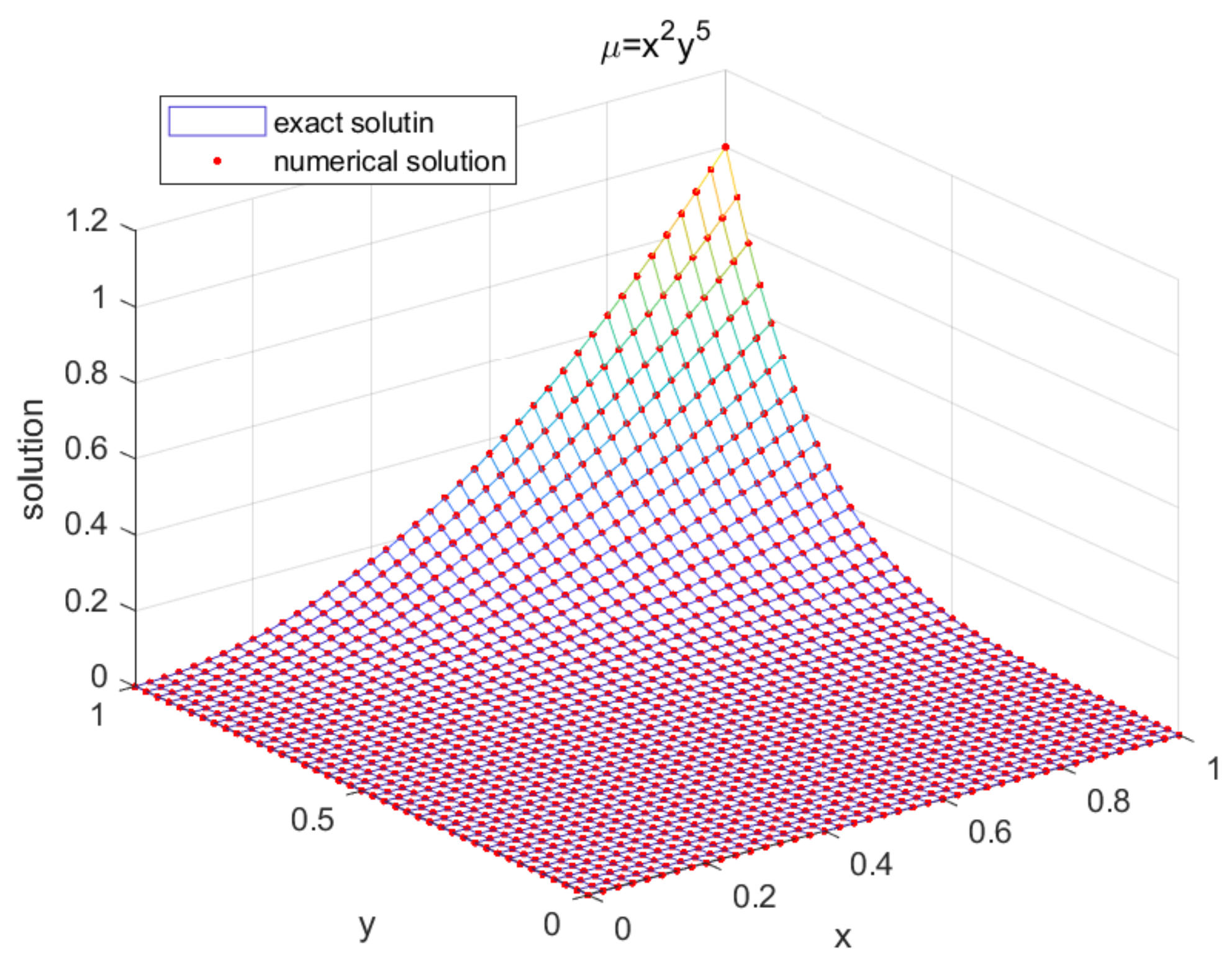
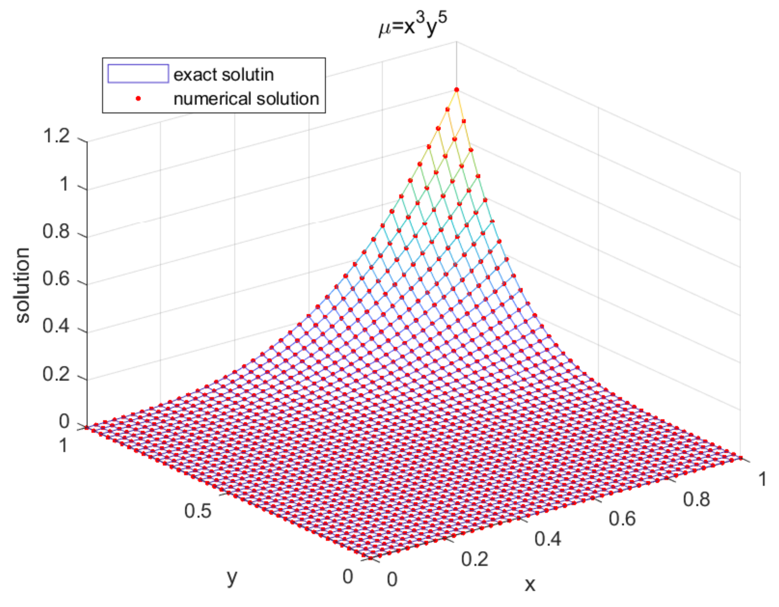
6. Numerical Examples

In this section, we use the higher-order numerical scheme (11) to solve the 3D-VIEs. The following four numerical examples are used to demonstrate the convergence order of the numerical solution. In the following numerical examples, we implement higher-order numerical scheme with $h=\frac{1}{N},N=5,10,20,40,80$ and error $E_h=\underset{i,j,q}{max}|\mu (x_i,y_j,z_q)-{\mu }_{i,j}^q|,i,j,q=0,1,\cdots ,N$. The convergence order is calculated by ${log}_2\left(\frac{E_{2h}}{E_h}\right)$. At the same time, without losing generality, we all choose the $\overline{g}=1$ to do the following analysis.

Example 1.

We consider the linear 3D-VIEs as follows:

$$\begin{array}{c}\hfill \mu (x,y,z)=g(x,y,z)+{\int }_0^x{\int }_0^y{\int }_0^z(xyz{w}^{2}t\nu )\mu (w,t,\nu )d\nu dtdw,(x,y,z)\in {[0,1]}^3,\end{array}$$

with the function g defined as

$$\begin{array}{c}\hfill g(x,y,z)=x^2{y}^5{z}^3-\frac{1}{175}{x}^6{y}^8{z}^6.\end{array}$$

It is straightforward to show that $\mu (x,y,z)=x^2{y}^5{z}^3$ is the exact solution of the above equation.

First, we perform numerical example according to the higher-order numerical solution in Section 3. According to different step lengths h, the calculated maximum absolute error and its convergence order are shown in

Table 1. Maximum errors and convergence rate as functions with h.

h	$\mathrm{Error}$	$\mathrm{Rate}$
$\frac{1}{5}$	$1.629551910207194\times {10}^{-4}$	−
$\frac{1}{10}$	$1.301070087844636\times {10}^{-5}$	$3.646704724239447$
$\frac{1}{20}$	$9.126369742151752\times {10}^{-7}$	$3.833513767270810$
$\frac{1}{40}$	$6.033795529880592\times {10}^{-8}$	$3.918903390618973$
$\frac{1}{80}$	$3.877251630868273\times {10}^{-9}$	$3.959959534894697$

.

The theoretical analysis results of Theorem 2 in Section 5 show that our optimal convergence order is 4 for our proposed higher-order numerical scheme. At the same time, through Table 1, we can know that when the value of $h=\frac{1}{5},\frac{1}{10},\frac{1}{20},\frac{1}{40},\frac{1}{80}$ gradually becomes smaller, the corresponding maximum absolute error also becomes smaller from ${10}^{-4}$ to ${10}^{-9}$, and the reduction is extremely obvious. In this process, we can know that our convergence order is gradually approaching 4.

Next, we show the distribution of function value for the numerical solution and the exact solution. The function value distribution of $N=80$ in the following Figure 1, where it is a comparison of the numerical solution and the exact solution corresponding to the 3D-VIEs. Figure 1 is the three-dimensional surface mesh map of the corresponding $\mu (x,y,1)=x^2{y}^5$ when $z=1$.

As can be seen from Figure 1, the numerical solution obtained by our calculation according to the numerical scheme is a good agreement with the exact solution of this example, and the values on the corresponding nodes are almost identical. Combining the data in Table 1 and Figure 1 in this example, we know that our proposed higher-order scheme has good convergence for linear 3D-VIE, which is consistent with the theoretical results.

Example 2.

Let us consider the following linear 3D-VIEs:

$$\begin{array}{c}\hfill \mu (x,y,z)=g(x,y,z)+{\int }_0^x{\int }_0^y{\int }_0^{z}sin(x-w){sin}^2(y+t)cos(2z+\nu )\mu (w,t,\nu )d\nu dtdw,\end{array}$$

where $(x,y,z)\in {[0,1]}^3$, and the function g is defined as

$$\begin{array}{cc}\hfill g(x,y,z)& =x^5{y}^2{z}^2-\left(x^5-20x^3+120x-120sin(x)\right)(\frac{1}{6}{y}^3-\frac{1}{4}{y}^{2}sin(4y)-\frac{1}{4}ycos(4y)\hfill \\ \hfill +& \frac{1}{8}sin(4y)-\frac{1}{8}sin(2y))\left(z^{2}sin(3z)+2zcos(3z)-2sin(3z)+2sin(2z)\right).\hfill \end{array}$$

The exact solution to the above equation is as follows:

$$\begin{array}{c}\hfill \mu (x,y,z)=x^5{y}^2{z}^2.\end{array}$$

In this example, we implement this calculation process to calculate the maximum absolute error and convergence order of the high-order numerical solution. According to different step sizes h, the maximum absolute error, and the convergence order can be obtained as shown in

Table 2. Maximum errors and convergence rate as functions with h.

h	$\mathrm{Error}$	$\mathrm{Rate}$
$\frac{1}{5}$	$1.306204365916219\times {10}^{-4}$	−
$\frac{1}{10}$	$1.122759745353363\times {10}^{-5}$	$3.540259485877905$
$\frac{1}{20}$	$8.162257019161956\times {10}^{-7}$	$3.781937294325425$
$\frac{1}{40}$	$5.490936638707922\times {10}^{-8}$	$3.893843971083792$
$\frac{1}{80}$	$3.558625838451235\times {10}^{-9}$	$3.947660105874005$

.

As can be seen from Table 2, when our step size h is $\frac{1}{5}$, the maximum absolute error of this numerical example is already very small, and the maximum absolute error at this time is about $1.3\times {10}^{-4}$. When $h=\frac{1}{80}$, the maximum absolute error is about $3.6\times {10}^{-9}$. At the same time, as h gradually decreases, the maximum absolute error becomes smaller and smaller. From the definition of the maximum absolute error, we can also know that the numerical solution in this numerical problem gradually approaches the exact solution when h becomes gradually smaller. From Table 2, we can roughly get that our numerical method is gradually approaching theoretical convergence order.

In the following, we will apply two nonlinear numerical examples to further demonstrate the conclusion of our Theorem 2.

Example 3.

We consider the following 3D nonlinear VIEs:

$$\begin{array}{c}\hfill \mu (x,y,z)=g(x,y,z)+{\int }_0^x{\int }_0^y{\int }_0^z(xyz+wt+{\nu }^2){\mu }^2(w,t,\nu )d\nu dtdw;(x,y,z)\in {[0,1]}^3,\end{array}$$

with the function g defined as

$$\begin{array}{c}\hfill g(x,y,z)=x^3{y}^5{z}^3-\frac{1}{539}{x}^8{y}^{12}{z}^8-\frac{1}{672}{x}^8{y}^{12}{z}^7-\frac{1}{693}{x}^7{y}^{11}{z}^9.\end{array}$$

It is easy to show that $\mu (x,y,z)=x^3{y}^5{z}^3$ is the corresponding exact solution of the above equation.

In order to show the theoretical analysis results of Theorem 2 for the 3D nonlinear VIE with a general kernel function, we choose a suitable h to indicate the corresponding maximum absolute error, and the maximum absolute error gradually decreases from ${10}^{-4}$ to ${10}^{-8}$. Among them, the step size h is the same as the selection of h in Example 1 and Example 2, and it gradually decreases from $\frac{1}{5}$ to $\frac{1}{80}$. Through some of numerical calculations, we obtain the relevant data of the 3D nonlinear VIEs as shown in the following

Table 3. Maximum errors and decay rate as functions with h.

h	$\mathrm{Error}$	$\mathrm{Rate}$
$\frac{1}{5}$	$9.194168478405818\times {10}^{-4}$	−
$\frac{1}{10}$	$8.959147119291799\times {10}^{-5}$	$3.359285798830145$
$\frac{1}{20}$	$7.183001882626883\times {10}^{-6}$	$3.640702600341250$
$\frac{1}{40}$	$5.105040028485774\times {10}^{-7}$	$3.814592715250178$
$\frac{1}{80}$	$3.399614900700954\times {10}^{-8}$	$3.908479037192826$

.

From Table 3, we have that the approximate solution of 3D nonlinear VIEs is convergent to the exact solution. Through a large number of tests, we can see the corresponding convergence order gradually approaches 4; that is to say, its optimal convergence order is 4. This is completely consistent with the theoretical analysis.

Next, we show the distribution of function value for the numerical solution and the exact solution. The function value distribution of $N=80$ in the following Figure 2, where it is a comparison of the numerical solution and the exact solution corresponding to the 3D-VIEs. Figure 2 shows the three-dimensional surface mesh map of the corresponding $\mu (x,y,1)=x^3{y}^5$ when $z=1$.

In Figure 2, we can hardly see the difference between the exact solution and the numerical solution of this numerical example. Therefore, we can draw the conclusion that the numerical solution of the nonlinear 3D-VIEs is very consistent with the exact solution, which also verifies the correctness of our theoretical analysis.

Example 4.

Let us consider the following 3D nonlinear VIEs with exponential form:

$$\begin{array}{c}\hfill \mu (x,y,z)=g(x,y,z)+{\int }_0^x{\int }_0^y{\int }_0^z{e}^{(x-w)+(y-t)+(z-\nu )}{\mu }^2(w,t,\nu )d\nu dtdw;(x,y,z)\in {[0,1]}^3,\end{array}$$

with the function g defined as

$$\begin{array}{cc}\hfill g(x,y,z)=& x^3{y}^4{z}^4-(-x^6-6x^5-30x^4-120x^3-360x^2-720x-720+720e^x)(-y^8\hfill \\ \hfill & -8y^7-56y^6-336y^5-1680y^4-6720y^3-20160y^2-40320y-40320\hfill \\ \hfill & +40320e^y)(-z^8-8z^7-56z^6-336z^5-1680z^4-6720z^3-20160z^2\hfill \\ \hfill & -40320z-40320+40320e^z),\hfill \end{array}$$

and the exact solution is $\mu (x,y,z)=x^3{y}^4{z}^4$.

In order to show the constructed numerical scheme’s good convergence, we will verify this example. The error $E_h$ and the convergence order of the solution of this 3D-VIE with respect to different h under the maximum norm of error are given in the following

Table 4. Maximum errors and decay rate as functions with h.

h	$\mathrm{Error}$	$\mathrm{Rate}$
$\frac{1}{5}$	$2.116544808936638\times {10}^{-4}$	−
$\frac{1}{10}$	$1.715380950773060\times {10}^{-5}$	$3.625110122038858$
$\frac{1}{20}$	$1.221438151288723\times {10}^{-6}$	$3.811876286531620$
$\frac{1}{40}$	$8.137970008981199\times {10}^{-8}$	$3.907768039330447$
$\frac{1}{80}$	$5.251625134761184\times {10}^{-9}$	$3.953833119346601$

.

It can be seen from Table 4 that the corresponding error is gradually decreasing with respect to h, and the convergence order of numerical scheme is 4.

Summarizing the linear and nonlinear 3D-VIEs described above, we know that the numerical method is convergent with the optimal convergence order of 4. They are completely consistent with the theoretical analysis results of Theorem 2.

7. Conclusions

A higher-order approximate solution for the nonlinear three-dimensional Volterra integral equation is presented in this paper. This numerical scheme is constructed by dividing the region into multiple subregions and applying cubic Lagrangian interpolation on each subregion. The scheme has uniform accuracy with an optimal convergence order of 4. We analyze the error generated by this numerical scheme through detailed steps, and use four numerical examples to verify that the error is within a reasonable range. Then it is concluded that this theoretical analysis is correct. In the future, we hope to construct a high-order approximate solution for a peridynamics plate model based on the idea of [29]. In addition, we intend to construct an efficient high-order numerical solution with uniform accuracy for 3D-VIEs with a generally weak nonlinear singular kernel function based on the ideas of [30,31]. Finally, we will apply a fast algorithm to implement the high-order numerical scheme for large-scale practical engineering problems based on the idea of [32].

References

1. El-Borai, M.; Abdou, M.; Badr, A.; Basseem, M. Singular nonlinear integral equation and its application in viscoelastic nonlinear material. Int. J. Appl. Math. Mech. 2008, 4, 56–77. [Google Scholar]
2. Brunner, H. Volterra Integral Equations: An Introduction to Theory and Applications; Cambridge University Press: New York, NY, USA, 2017. [Google Scholar]
3. Souchet, R. An analysis of three-dimensional rigid body collisions with friction by means of a linear integral equation of Volterra. Internat. J. Engrg. Sci. 1999, 37, 365–378. [Google Scholar] [CrossRef]
4. Katani, R.; Shahmorad, S. Block by block method for the systems of nonlinear Volterra integral equations. Appl. Math. Model. 2009, 34, 400–406. [Google Scholar] [CrossRef]
5. Tao, T.; Xu, X.; Cheng, J. On spectral methods for Volterra integral equations and the convergence analysis. J. Comput. Math. 2008, 26, 825–837. [Google Scholar]
6. Maleknejad, K.; Aghazadeh, N. Numerical solution of Volterra integral equations of the second kind with convolution kernel by using Taylor-series expansion method. Appl. Math. Comput. 2003, 161, 915–922. [Google Scholar] [CrossRef]
7. Jaabar, S.; Hussain, A. Solving Volterra integral equation by using a new transformation. J. Interdiscip. Math. 2021, 24, 735–741. [Google Scholar] [CrossRef]
8. Bazm, S.; Lima, P.; Nemati, S. Analysis of the Euler and trapezoidal discretization methods for the numerical solution of nonlinear functional Volterra integral equations of Urysohn type. J. Comput. Appl. Math. 2021, 398, 113628. [Google Scholar] [CrossRef]
9. Cao, J.; Xu, C. A high order schema for the numerical solution of the fractional ordinary differential equations. J. Comput. Phys. 2013, 238, 154–168. [Google Scholar] [CrossRef]
10. Cao, J.; Cai, Z. Numerical analysis of a high-order scheme for nonlinear fractional difffferential equations with uniform accuracy. Numer. Math. Theor. Meth. Appl. 2021, 14, 71–112. [Google Scholar] [CrossRef]
11. Wu, C.; Wang, Z. The spectral collocation method for solving a fractional integro-differential equation. AIMS Math. 2021, 6, 9577–9587. [Google Scholar] [CrossRef]
12. Maleknejad, K.; Hashemizadeh, E.; Ezzati, R. A new approach to the numerical solution of Volterra integral equations by using Bernstein’s approximation. Commun. Nonlinear Sci. Numer. Simul. 2011, 16, 647–655. [Google Scholar] [CrossRef]
13. Rahma, A.; Evans, D. The numerical solution of Volterra integral equations on parallel computers. Int. J. Comput. Math. 2007, 27, 103–111. [Google Scholar] [CrossRef]
14. Maleknejad, K.; Basirat, B.; Hashemizadeh, E. A Bernstein operational matrix approach for solving a system of high order linear Volterra-Fredholm integro-differential equations. Math. Comput. Model. 2012, 55, 1363–1372. [Google Scholar] [CrossRef]
15. Odibat, Z. Differential transform method for solving Volterra integral equation with separable kernels. Math. Comput. Model. 2008, 48, 1144–1149. [Google Scholar] [CrossRef]
16. Assari, P.; Dehghan, M. The approximate solution of nonlinear Volterra integral equations of the second kind using radial basis functions. Appl. Numer. Math. 2018, 131, 140–157. [Google Scholar] [CrossRef]
17. Han, G.; Hayami, K.; Sugihara, K.; Wang, J. Extrapolation method of iterated collocation solution for two-dimensional nonlinear Volterra integral equations. Appl. Math. Comput. 2000, 112, 49–61. [Google Scholar]
18. McKee, S.; Tang, T.; Diogo, T. An Euler-type method for two-dimensional Volterra integral equations of the first kind. IMA J. Numer. Anal. 2000, 20, 423–440. [Google Scholar] [CrossRef]
19. Tari, A.; Rahimi, M.; Shahmorad, S.; Talati, F. Solving a class of two-dimensional linear and nonlinear Volterra integral equations by the differential transform method. J. Comput. Appl. Math. 2009, 228, 70–76. [Google Scholar] [CrossRef]
20. Maleknejad, K.; Rashidinia, J.; Eftekhari, T. Existence, uniqueness, and numerical solutions for two-dimensional nonlinear fractional Volterra and Fredholm integral equations in a Banach space. Comput. Appl. Math. 2020, 39, 1–22. [Google Scholar] [CrossRef]
21. Assari, P.; Dehghan, M. A meshless local discrete Galerkin (MLDG) scheme for numerically solving two-dimensional nonlinear Volterra integral equations. Appl. Math. Comput. 2019, 350, 249–265. [Google Scholar] [CrossRef]
22. Wang, Y.; Huang, J.; Wen, X. Two-dimensional Euler polynomials solutions of two-dimensional Volterra integral equations of fractional order. Appl. Numer. Math. 2021, 163, 77–95. [Google Scholar] [CrossRef]
23. Khosrow, M.; Jalil, R.; Tahereh, E. Numerical solution of three-dimensional Volterra-Fredholm integral equations of the first and second kinds based on Bernstein’s approximation. Appl. Math. Comput. 2018, 339, 272–285. [Google Scholar]
24. Zaky, M.; Ameen, I. A novel Jacob spectral method for multi-dimensional weakly singular nonlinear Volterra integral equations with nonsmooth solutions. Eng. Comput. 2021, 37, 2623–2631. [Google Scholar] [CrossRef]
25. Ziqan, A.; Armiti, S.; Suwan, I. Solving three-dimensional Volterra integral equation by the reduced differential transform method. Int. J. Appl. Math. Res. 2016, 5, 103–106. [Google Scholar] [CrossRef] [Green Version]
26. Bakhshi, M. Three-dimensional differential transform method for solving nonlinear three-dimensional Volterra integral equations. Int. J. Appl. Math. Comput. Sci. 2012, 4, 246–256. [Google Scholar] [CrossRef]
27. Nawaz, R.; Ahsan, S.; Akbar, M.; Farooq, M.; Sulaiman, M.; Ullah, H.; Islam, S. Semi analytical solutions of second type of three-dimensional Volterra integral equations. Int. J. Appl. Comput. Math. 2020, 6, 3079–3096. [Google Scholar] [CrossRef]
28. Mirzaee, F.; Hadadiyan, E.; Bimesl, S. Numerical solution for three-dimensional nonlinear mixed Volterra-Fredholm integral equations via three-dimensional block-pulse functions. Appl. Math. Comput. 2014, 237, 168–175. [Google Scholar] [CrossRef]
29. Wang, Z.; Cui, J. Second-order two-scale method for bending behavior analysis of composite plate with 3-D periodic configuration and its approximation. Sci. China Math. 2014, 57, 1713–1732. [Google Scholar] [CrossRef]
30. Wang, Z.; Liu, Q.; Cao, J. A higher-order numerical scheme for two-dimensional nonlinear fractional Volterra integral equations with uniform accuracy. Fractal Fract. 2022, 6, 314. [Google Scholar] [CrossRef]
31. Cao, J.; Zhang, J.; Yang, X. Fully-discrete Spectral-Galerkin scheme with second-order time-accuracy and unconditionally energy stability for the volume-conserved phase-field lipid vesicle model. J. Comput. Appl. Math. 2022, 406, 113988. [Google Scholar] [CrossRef]
32. Gu, X.; Wu, S. A parallel-in-time iterative algorithm for Volterra partial integro-differential problems with weakly singular kernel. J. Comput. Phys. 2022, 417, 109576. [Google Scholar] [CrossRef]
Figure 1. Comparison of numerical and exact solutions.
Axioms 11 00476 g001
Figure 2. Comparison of numerical and exact solutions.
Axioms 11 00476 g002