Article

Stability of a Nonlinear ML-Nonsingular Kernel Fractional Langevin System with Distributed Lags and Integral Control

Department of Mathematics, School of Electronics & Information Engineering, Taizhou University, Taizhou 318000, China
Axioms 2022, 11(7), 350; https://doi.org/10.3390/axioms11070350
Submission received: 21 June 2022 / Revised: 16 July 2022 / Accepted: 18 July 2022 / Published: 21 July 2022
(This article belongs to the Special Issue Numerical Methods for Fractional and Integer PDEs)

Abstract

:
The fractional Langevin equation has more advantages than its classical equation in representing the random motion of Brownian particles in complex viscoelastic fluid. The Mittag–Leffler (ML) fractional equation without singularity is more accurate and effective than Riemann–Caputo (RC) and Riemann–Liouville (RL) fractional equation in portraying Brownian motion. This paper focuses on a nonlinear ML-fractional Langevin system with distributed lag and integral control. Employing the fixed-point theorem of generalised metric space established by Diaz and Margolis, we built the Hyers–Ulam–Rassias (HUR) stability along with Hyers–Ulam (HU) stability of this ML-fractional Langevin system. Applying our main results and MATLAB software, we have carried out theoretical analysis and numerical simulation on an example. By comparing with the numerical simulation of the corresponding classical Langevin system, it can be seen that the ML-fractional Langevin system can better reflect the stationarity of random particles in the statistical sense.

1. Introduction

In 1908, Langevin raised the famous Langevin equation to reveal the dynamics of random motion of particles in fluid. The classical Langevin equation [1] of Brownian particle is formulated by
m d 2 S d t 2 + ε d S d t = f ( t , S ( t ) ) ,
where S ( t ) is the particle’s position, m expresses the particle’s mass, ε represents a speed’s proportional coefficient, f is the external force of fluid molecules acting on the Brownian particle. Afterward, many random phenomena and processes were found to be described by Langevin equation [2,3]. However, when using classical Langevin equation to describe complex viscoelasticity, there is a large deviation from the experimental results. This prompted some researchers to modify and generalise the classical Langevin equation. Kubo [4,5] advanced a general Langevin equation to simulate the complex viscoelastic anomalous diffusion process. Eab and Lim [6] introduced a fractional Langevin equation to describe the single-file diffusion. Sandev and Tomovski [7] also set up a fractional Langevin equation model to study the motion of free particles driven by power-law noise. In addition, readers can find the latest research progress of fractional Langevin systems in recent papers [8,9].
As we all know, the stability of the system is of vital important for the application of the system in practice. In 1940s, Hyers and Ulam [10,11] proposed a concept of system stability called HU-stability. In recent ten years, there have many works (some of them [12,13,14,15,16,17]) on HU-stability of fractional system. However, these research findings on fractional Langevin system are all about RC- or RL-fractional derivative. Unfortunately, the RC- and RL-fractional derivatives will produce singularity under some conditions. So the RC- and RL-fractional models are defective in describing some physical phenomena. Consequently, Caputo and Febrizio [18] raised a new exponential kernel nonsingular fractional derivative. And another new nonsingular fractional derivative with ML-kernel is put forward by Atangana and Baleanu in [19]. These nonsingular fractional derivatives have attracted much attention and research in theory [20,21,22,23,24] and application [25,26,27,28,29,30] since they were proposed. As far as we are concerned, there are no papers on UH-type stability of ML-fractional Langevin system. Awaken by above mentioned, this paper primarily concerns a nonlinear ML-fractional Langevin system with distributed lag and integral control written by
M L D 0 + ν M L D 0 + μ λ U ( x ) = f x , ( I 1 U ) ( x ) , ( I 2 U ) ( x ) , x ( 0 , T ] , ( I 1 U ) ( x ) = σ 1 ( x ) 0 k ( s ) U ( x + s ) d s , ( I 2 U ) ( x ) = 0 x U ( s ) d H ( s ) , x J = [ 0 , T ] , U ( x ) = ω 1 ( x ) , M L D 0 + μ U ( x ) = ω 2 ( x ) , x [ σ , 0 ] ,
where T , μ , ν and λ are some constants with T > 0 , 0 < μ , ν 1 and λ > 0 , M L D 0 + expresses the ∗-order ML-fractional derivative, the nonlinear function f C ( J × R 2 , R ) , the time-lag function σ 1 C ( J , R + ) with σ = max x J σ 1 ( x ) , the initial function ω j C ( [ σ , 0 ] , R ) ( j = 1 , 2 ) , the distributed lag kernel function k ( s ) C ( [ σ , 0 ] , R + ) , the integral control ( I 2 U ) ( x ) is Riemann–Stieltjes integral, H : [ 0 , T ] R is the function of bounded variation.
The organizational structure of the remaining sections of the manuscript is as below. Section 2 introduces the basic knowledge and results of ML-fractional calculus used later. The HUR-, GHUR-, HU- and HUR-stability of (1) are established by Diaz and Margolis’s fixed-point theorem in Section 3. As an application, the theoretical analysis and numerical simulation on an example are conducted in Section 4. Section 4.2 is a brief conclusion.

2. Preliminaries

Definition 1
([31]). For 0 < μ 1 , T > 0 and U : [ 0 , T ] R , the left-sided μ-order Mittag–Leffler fractional integral of function U is defined by
M L J 0 + μ U ( x ) = 1 μ N ( μ ) U ( x ) + μ N ( μ ) Γ ( μ ) 0 x ( x s ) μ 1 U ( s ) d s ,
provided the integral exists, here Γ ( μ ) = 0 s μ 1 e s d s , N ( μ ) is a normalization constant satisfying N ( 0 ) = N ( 1 ) = 1 .
Definition 2
([19]). For 0 < μ 1 , T > 0 and U C 1 ( 0 , T ) , the left-sided μ-order Mittag–Leffler fractional derivative of function u in sense of Caputo is given by
M L D 0 + μ U ( x ) = N ( μ ) ( 1 μ ) 0 x E μ μ 1 μ ( x s ) μ U ( s ) d s ,
where E μ ( · ) is single parameter Mittag-Leffler function and defines as
E μ ( z ) = n = 0 z n Γ ( μ k + 1 ) .
Lemma 1
([20]). Assume that h C [ 0 , T ] . Then the unique solution of below ML-fractional system
M L D 0 + p y ( x ) = h ( x ) , x ( 0 , T ) , 0 < p 1 , w ( 0 ) = w 0 ,
is written as
y ( x ) = y 0 + 1 p N ( p ) [ h ( x ) h ( 0 ) ] + p N ( p ) Γ ( p ) 0 x ( x s ) p 1 h ( s ) d s .
Remark 1.
From Definition 2 and Lemma 1, one easily concludes that M L D 0 + μ U ( x ) 0 iff U ( x ) constant .
Lemma 2.
Let T > 0 , J = [ 0 , T ] , 0 < μ , ν 1 , λ > 0 , f C ( J × R 2 , R ) , σ 1 C ( J , R + ) with σ = max x J σ 1 ( x ) , ω j C ( [ σ , 0 ] , R ) ( j = 1 , 2 ) , k ( s ) C ( [ σ , 0 ] , R + ) , the integral control ( I 2 U ) ( x ) be Riemann–Stieltjes integral, and H : [ 0 , T ] R be the function of bounded variation. If Δ 1 λ ( 1 μ ) N ( μ ) 0 , then the nonlinear ML-fractional Langevin system (1) is equivalent to the below delayed nonlinear integral system
U ( x ) = ω 1 ( 0 ) + 1 Δ { ω 2 ( 0 ) λ ω 1 ( 0 ) N ( μ ) Γ ( μ ) x μ ( 1 μ ) ( 1 ν ) N ( μ ) N ( ν ) F U ( 0 ) + ( 1 μ ) ( 1 ν ) N ( μ ) N ( ν ) F U ( x ) + λ μ N ( μ ) Γ ( μ ) 0 x ( x s ) μ 1 U ( s ) d s + ( 1 μ ) ν N ( μ ) N ( ν ) Γ ( ν ) 0 x ( x s ) ν 1 F U ( s ) d s + μ ( 1 ν ) N ( μ ) N ( ν ) Γ ( μ ) 0 x ( x s ) μ 1 F U ( s ) d s + μ ν N ( μ ) N ( ν ) Γ ( μ + ν ) 0 x ( x s ) μ + ν 1 F U ( s ) d s } , x J , ω 1 ( x ) , x [ σ , 0 ] ,
where F U ( x ) = f ( x , ( I 1 U ) ( x ) , ( I 2 U ) ( x ) ) , ( I 1 U ) ( x ) = σ 1 ( x ) 0 k ( s ) U ( x + s ) d s , ( I 2 U ) ( x ) = 0 x U ( s ) d H ( s ) .
Proof. 
Let V ( x ) = M L D 0 + μ λ U ( x ) , then the first equation of (1) is changed into
M L D 0 + ν V ( x ) = f ( x , ( I 1 U ) ( x ) , ( I 2 U ) ( x ) ) , x ( 0 , T ] , M L D 0 + μ U ( x ) = λ U ( x ) + V ( x ) , x ( 0 , T ] .
On the one hand, assume that U ( x ) is a solution of (1), where U C 1 [ 0 , T ] . Then, for x J = [ 0 , T ] , one derives from Lemma 1 and (3) that
V ( x ) = V ( 0 ) + 1 ν N ( ν ) f ( x , ( I 1 U ) ( x ) , ( I 2 U ) ( x ) ) f ( 0 , ( I 1 U ) ( 0 ) , ( I 2 U ) ( 0 ) ) + ν N ( ν ) Γ ( ν ) 0 x ( x ζ ) ν 1 f ( ζ , ( I 1 U ) ( ζ ) , ( I 2 U ) ( ζ ) ) d ζ ,
and
U ( x ) = U ( 0 ) + 1 μ N ( μ ) λ [ U ( x ) U ( 0 ) ] + [ V ( x ) V ( 0 ) ] + μ N ( μ ) Γ ( μ ) 0 x ( x s ) μ 1 [ λ U ( s ) + V ( s ) ] d s .
Together with (4) and (5) and initial conditions U ( 0 ) = ω 1 ( 0 ) and V ( 0 ) = M L D 0 + μ U ( 0 ) λ U ( 0 ) = ω 2 ( 0 ) λ ω 1 ( 0 ) , one gets
U ( x ) = ω 1 ( 0 ) + 1 μ N ( μ ) [ λ [ U ( x ) ω 1 ( 0 ) ] + 1 ν N ( ν ) [ f ( x , ( I 1 U ) ( x ) , ( I 2 U ) ( x ) ) f ( 0 , ( I 1 U ) ( 0 ) , ( I 2 U ) ( 0 ) ) ] + ν N ( ν ) Γ ( ν ) 0 x ( x ζ ) ν 1 f ( ζ , ( I 1 U ) ( ζ ) , ( I 2 U ) ( ζ ) ) d ζ ] + μ N ( μ ) Γ ( μ ) 0 x ( x s ) μ 1 [ ( ω 2 ( 0 ) λ ω 1 ( 0 ) ) + λ U ( s ) + 1 ν N ( ν ) f ( s , ( I 1 U ) ( s ) , ( I 2 U ) ( s ) ) + ν N ( ν ) Γ ( ν ) 0 s ( s ζ ) ν 1 f ( ζ , ( I 1 U ) ( ζ ) , ( I 2 U ) ( ζ ) ) d ζ ] d s = 1 λ ( 1 μ ) N ( μ ) ω 1 ( 0 ) + λ ( 1 μ ) N ( μ ) U ( x ) + ( 1 μ ) ( 1 ν ) N ( μ ) N ( ν ) [ f ( x , ( I 1 U ) ( x ) , ( I 2 U ) ( x ) ) f ( 0 , ( I 1 U ) ( 0 ) , ( I 2 U ) ( 0 ) ) ] + ( 1 μ ) ν N ( μ ) N ( ν ) Γ ( ν ) 0 x ( x ζ ) ν 1 f ( ζ , ( I 1 U ) ( ζ ) , ( I 2 U ) ( ζ ) ) d ζ + ω 2 ( 0 ) λ ω 1 ( 0 ) N ( μ ) Γ ( μ ) x μ + λ μ N ( μ ) Γ ( μ ) 0 x ( x s ) μ 1 U ( s ) d s + μ ( 1 ν ) N ( μ ) N ( ν ) Γ ( μ ) × 0 x ( x s ) μ 1 f ( s , ( I 1 U ) ( s ) , ( I 2 U ) ( s ) ) d s + μ ν N ( μ ) N ( ν ) Γ ( μ ) Γ ( ν ) × 0 x ( x s ) μ 1 0 s ( s ζ ) ν 1 f ( ζ , ( I 1 U ) ( ζ ) , ( I 2 U ) ( ζ ) ) d ζ d s .
Exchanged the order of integrals, the last quadratic integral of (6) is computed as
0 x ( x s ) μ 1 0 s ( s ζ ) ν 1 f ( ζ , ( I 1 U ) ( ζ ) , ( I 2 U ) ( ζ ) ) d ζ d s = 0 x f ( ζ , ( I 1 U ) ( ζ ) , ( I 2 U ) ( ζ ) ) ζ x ( x s ) μ 1 ( s ζ ) ν 1 d s d ζ = Γ ( μ ) Γ ( ν ) Γ ( μ + ν ) 0 x ( x ζ ) μ + ν 1 f ( ζ , ( I 1 U ) ( ζ ) , ( I 2 U ) ( ζ ) ) d ζ .
From (6) and (7), one has
U ( x ) = ω 1 ( 0 ) + 1 Δ { ω 2 ( 0 ) λ ω 1 ( 0 ) N ( μ ) Γ ( μ ) x μ ( 1 μ ) ( 1 ν ) N ( μ ) N ( ν ) f ( 0 , ( I 1 U ) ( 0 ) , ( I 2 U ) ( 0 ) ) + ( 1 μ ) ( 1 ν ) N ( μ ) N ( ν ) f ( x , ( I 1 U ) ( x ) , ( I 2 U ) ( x ) ) + λ μ N ( μ ) Γ ( μ ) 0 x ( x s ) μ 1 U ( s ) d s + ( 1 μ ) ν N ( μ ) N ( ν ) Γ ( ν ) 0 x ( x ζ ) ν 1 f ( ζ , ( I 1 U ) ( ζ ) , ( I 2 U ) ( ζ ) ) d ζ + μ ( 1 ν ) N ( μ ) N ( ν ) Γ ( μ ) 0 x ( x ζ ) μ 1 f ( ζ , ( I 1 U ) ( ζ ) , ( I 2 U ) ( ζ ) ) d ζ + μ ν N ( μ ) N ( ν ) Γ ( μ + ν ) 0 x ( x ζ ) μ + ν 1 f ( ζ , ( I 1 U ) ( ζ ) , ( I 2 U ) ( ζ ) ) d ζ } = ω 1 ( 0 ) + 1 Δ { ω 2 ( 0 ) λ ω 1 ( 0 ) N ( μ ) Γ ( μ ) x μ ( 1 μ ) ( 1 ν ) N ( μ ) N ( ν ) F U ( 0 ) + ( 1 μ ) ( 1 ν ) N ( μ ) N ( ν ) F U ( x ) + λ μ N ( μ ) Γ ( μ ) 0 x ( x s ) μ 1 U ( s ) d s + ( 1 μ ) ν N ( μ ) N ( ν ) Γ ( ν ) 0 x ( x ζ ) ν 1 F U ( ζ ) d ζ + μ ( 1 ν ) N ( μ ) N ( ν ) Γ ( μ ) 0 x ( x ζ ) μ 1 F U ( ζ ) d ζ + μ ν N ( μ ) N ( ν ) Γ ( μ + ν ) 0 x ( x ζ ) μ + ν 1 F U ( ζ ) d ζ } .
Obviously, Equation (8) is the first equation of (2). When x [ σ , 0 ] , it is evident that U ( x ) = ω 1 ( x ) holds. So far, we have fully derived the delayed integral Equation (2). That is, U ( x ) is also a solution of delayed integral Equation (2).
On the other hand, when x [ σ , 0 ] , let’s make a supplementary definition M L D 0 + μ U ( x ) = ω 2 ( x ) , then U ( x ) = ω 1 ( x ) and M L D 0 + μ U ( x ) = ω 2 ( x ) satisfy the system (2) ⇒ U ( x ) = ω 1 ( x ) and M L D 0 + μ U ( x ) = ω 2 ( x ) satisfy the system (1). When x J , if U ( x ) with U C 1 [ 0 , T ] is a solution of delayed integral Equation (2), then we take ν -order ML-fractional derivative of (4) and μ -order ML-fractional derivative of (5) to get the second equation of (1) and (3), respectively. Thus we verify that U ( x ) with U C 1 [ 0 , T ] is also a solution of the first equation in system (1). The proof is completed. □
Definition 3.
Let D ( · , · ) be a binary function defined on a nonempty set Y . If D ( · , · ) satisfies
(1)
nonnegativity, i.e., D ( ξ , η ) 0 , and the identity holds only if ξ = η , ξ , η Y ;
(2)
commutativity, i.e., D ( ξ , η ) = D ( η , ξ ) , ξ , η Y ;
(3)
trigonometric inequality, i.e., D ( ξ , η ) D ( ξ , ζ ) + D ( ζ , η ) , ξ , η , ζ Y .
Then ( Y , D ) is called a generalised metric space.
Lemma 3
(Diaz and Margolis [32]). Let ( Y , D ) be a complete generalised metric space, and T : Y Y be a mapping. Assume that the following conditions hold:
(a)
For all ξ , η Y , there exists a constant 0 < ρ < 1 such that D ( T ξ , T η ) < ρ D ( ξ , η ) ;
(b)
For some ξ Y , there exists an integer m 0 such that D ( T m + 1 ξ , T m ξ ) < + .
Then the below assertions are true:
(i)
D ( T n ξ , ξ ) 0 , as n , and T ξ = ξ ;
(ii)
There exists a unique ξ Y = { η Y : D ( T m ξ , η ) < } such that T ξ = ξ ;
(iii)
If η Y , then D ( η , ξ ) 1 1 ρ D ( T η , η ) .

3. Existence and Stability

In this section, we will apply Lemma 3 to prove the UHR, GUHR, UH and GUH stability for system (1). Take Y = C ( [ σ , T ] , R ) , Based on Lemma 2, a mapping T : Y Y is introduced as follows:
( T U ) ( x ) = ω 1 ( 0 ) + 1 Δ { ω 2 ( 0 ) λ ω 1 ( 0 ) N ( μ ) Γ ( μ ) x μ ( 1 μ ) ( 1 ν ) N ( μ ) N ( ν ) F U ( 0 ) + ( 1 μ ) ( 1 ν ) N ( μ ) N ( ν ) F U ( x ) + λ μ N ( μ ) Γ ( μ ) 0 x ( x s ) μ 1 U ( s ) d s + ( 1 μ ) ν N ( μ ) N ( ν ) Γ ( ν ) 0 x ( x s ) ν 1 F U ( s ) d s + μ ( 1 ν ) N ( μ ) N ( ν ) Γ ( μ ) 0 x ( x s ) μ 1 F U ( s ) d s + μ ν N ( μ ) N ( ν ) Γ ( μ + ν ) 0 x ( x s ) μ + ν 1 F U ( s ) d s } , x J , ω 1 ( x ) , x [ σ , 0 ] ,
where F U ( x ) = f ( x , ( I 1 U ) ( x ) , ( I 2 U ) ( x ) ) , ( I 1 U ) ( x ) = σ 1 ( x ) 0 k ( s ) U ( x + s ) d s , ( I 2 U ) ( x ) = 0 x U ( s ) d H ( s ) .
Let W Y , ϵ > 0 , 0 < μ , ν 1 and φ C ( J , R + ) be non-decreasing. Consider the following two inequalities
| M L D 0 + ν M L D 0 + μ λ W ( x ) f ( x , ( I 1 W ) ( x ) , ( I 2 W ) ( x ) ) | ϵ , 0 < x T , W ( x ) = ω 1 ( x ) , M L D 0 + μ W ( x ) = ω 2 ( x ) , x [ σ , 0 ] ,
and
| M L D 0 + ν M L D 0 + μ λ W ( x ) f ( x , ( I 1 W ) ( x ) , ( I 2 W ) ( x ) ) | ϵ φ ( x ) , 0 < x T , W ( x ) = ω 1 ( x ) , M L D 0 + μ W ( x ) = ω 2 ( x ) , x [ σ , 0 ] ,
Definition 4.
The problem (1) is Hyers–Ulam (HU) stable, if ϵ > 0 and any solution W Y of (10), there have a unique solution U Y of (1) and a constant C 1 > 0 satisfying
| W ( x ) U ( x ) | C 1 ϵ .
Definition 5.
The problem (1) is generalised Hyers–Ulam (GHU) stable, if ϵ > 0 and any solution W Y of (10), there have a unique solution U Y of (1) and function θ ( · ) C ( R , R + ) with θ ( 0 ) = 0 satisfying
| W ( x ) U ( x ) | θ ( ϵ ) .
Definition 6.
The problem (1) is Hyers–Ulam–Rassias (HUR) stable, if ϵ > 0 and any solution W Y of (11), there have a unique solution U Y of (1) and constant C 2 > 0 satisfying
| W ( x ) U ( x ) | C 2 φ ( x ) ϵ , x [ σ , T ] .
Definition 7.
The problem (1) is generalised Hyers–Ulam–Rassias (GHUR) stable, if for any solution W Y of (11), there have a unique solution U Y of (1) and constant C 3 > 0 satisfying
| W ( x ) U ( x ) | C 3 φ ( x ) , x [ σ , T ] .
Obviously, HU stable ⇒ GHU stable, and HUR stable ⇒ GHUR stable.
Remark 2.
A function W Y satisfies the inequality (10) iff there has ϕ C ( 0 , T ] × C ( 0 , T ] satisfying
(1)
| ϕ ( x ) | ϵ , 0 < x T ;
(2)
M L D 0 + ν M L D 0 + μ λ W ( x ) = f ( x , ( I 1 W ) ( x ) , ( I 2 W ) ( x ) ) + ϕ ( x ) , 0 < x T ;
(3)
W ( x ) = ω 1 ( x ) , M L D 0 + μ W ( x ) = ω 2 ( x ) , x [ σ , 0 ] .
Remark 3.
A function W Y satisfies the inequality (11) iff there has ψ C ( 0 , T ] × C ( 0 , T ] satisfying
(1)
| ψ ( x ) | ϵ φ ( x ) , 0 < x T ;
(2)
M L D 0 + ν M L D 0 + μ λ W ( x ) = f ( x , ( I 1 W ) ( x ) , ( I 2 W ) ( x ) ) + ψ ( x ) , 0 < x T ;
(3)
W ( x ) = ω 1 ( x ) , M L D 0 + μ W ( x ) = ω 2 ( x ) , x [ σ , 0 ] .
(B1)
T , μ , ν , λ are some constants and satisfy T , λ > 0 , 0 < μ , ν 1 , and Δ 1 λ ( 1 μ ) N ( μ ) 0 ;
(B2)
f C ( J × R 2 , R ) , σ 1 C ( J , R + ) , σ = max x J σ 1 ( x ) , ω j C ( [ σ , 0 ] , R ) ( j = 1 , 2 ) , k ( s ) C ( [ σ , 0 ] , R + ) , the integral control ( I 2 U ) ( x ) be Riemann–Stieltjes integral, and H : [ 0 , T ] R be the bounded variation;
(B3)
x J , U , U ¯ , Z , Z ¯ R , there have two functions L 1 ( x ) , L 2 ( x ) C ( J , R + ) satisfying
| f ( x , U , Z ) | f ( x , U ¯ , Z ¯ ) | L 1 ( x ) | U U ¯ | + L 2 ( x ) | Z Z ¯ | ;
(B4)
0 < Θ < 1 , where Θ = λ T μ | Δ | N ( μ ) Γ ( μ ) + ϱ | Δ | N ( μ ) N ( ν ) 2 ( 1 μ ) ( 1 ν ) + ( 1 μ ) T ν Γ ( ν ) + ( 1 ν ) T μ Γ ( μ ) + μ ν T μ + ν Γ ( μ + ν + 1 ) , ϱ = L 1 T σ 0 k ( s ) d s + L 2 T 0 T d H ( s ) and · T = max x [ 0 , T ] | · | .
Theorem 1.
If the conditions ( B 1 ) ( B 4 ) are true, then system (1) is HUR stable and also GHUR stable.
Proof. 
By Definition 6, similar to the Theorem 3.1 in [33], we introduce a complete generalised metric space ( Y , D ) , where Y = C ( [ σ , T ] , R ) and
D ( U , W ) = inf { M [ 0 , ] : | U ( x ) W ( x ) | M φ ( x ) , x [ σ , T ] } .
A mapping T : Y Y is defined as (9). Based on the conditions ( B 1 ) and ( B 2 ) , one knows that T is well defined.
Firstly, U , W Y , when x [ σ , 0 ] , one has
| ( T U ) ( x ) ( T W ) ( x ) | = | ω 1 ( x ) ω 1 ( x ) | 0 .
When x J = [ 0 , T ] , noting that D ( U , W ) = M , (12) gives
| U ( x ) W ( x ) | M φ ( x ) .
In addition, by ( B 3 ) , (9) and (14), one has
| F U ( x ) F W ( x ) | = | f ( x , ( I 1 U ) ( x ) , ( I 2 U ) ( x ) ) f ( x , ( I 1 W ) ( x ) , ( I 2 W ) ( x ) ) | L 1 ( x ) | ( I 1 U ) ( x ) ( I 1 W ) ( x ) | + L 2 ( x ) | ( I 2 U ) ( x ) ) ( I 2 W ) ( x ) ) | L 1 T σ 1 ( x ) 0 k ( s ) | U ( x + s ) W ( x + s ) | d s + L 2 T 0 x | U ( s ) W ( s ) | d H ( s ) L 1 T σ 0 k ( s ) | U ( x + s ) W ( x + s ) | d s + L 2 T 0 x | U ( s ) W ( s ) | d H ( s ) L 1 T σ 0 k ( s ) d s + L 2 T 0 T d H ( s ) M φ ( x ) = ϱ M φ ( x ) .
Noticing that φ C ( J , R + ) is non-decreasing, in view of (9), (14) and (15), one yields
| ( T U ) ( x ) ( T W ) ( x ) | = 1 | Δ | | ( 1 μ ) ( 1 ν ) N ( μ ) N ( ν ) [ F U ( 0 ) F W ( 0 ) ] + ( 1 μ ) ( 1 ν ) N ( μ ) N ( ν ) [ F U ( x ) F W ( x ) ] + λ μ N ( μ ) Γ ( μ ) 0 x ( x s ) μ 1 [ U ( s ) W ( s ) ] d s + ( 1 μ ) ν N ( μ ) N ( ν ) Γ ( ν ) 0 x ( x s ) ν 1 [ F U ( s ) F W ( s ) ] d s + μ ( 1 ν ) N ( μ ) N ( ν ) Γ ( μ ) 0 x ( x s ) μ 1 [ F U ( s ) F W ( s ) ] d s + μ ν N ( μ ) N ( ν ) Γ ( μ + ν ) 0 x ( x s ) μ + ν 1 [ F U ( s ) F W ( s ) ] d s | 1 | Δ | [ ( 1 μ ) ( 1 ν ) N ( μ ) N ( ν ) | F U ( 0 ) F W ( 0 ) | + ( 1 μ ) ( 1 ν ) N ( μ ) N ( ν ) | F U ( x ) F W ( x ) | + λ μ N ( μ ) Γ ( μ ) 0 x ( x s ) μ 1 | U ( s ) W ( s ) | d s + ( 1 μ ) ν N ( μ ) N ( ν ) Γ ( ν ) 0 x ( x s ) ν 1 | F U ( s ) F W ( s ) | d s + μ ( 1 ν ) N ( μ ) N ( ν ) Γ ( μ ) 0 x ( x s ) μ 1 | F U ( s ) F W ( s ) | d s + μ ν N ( μ ) N ( ν ) Γ ( μ + ν ) 0 x ( x s ) μ + ν 1 | F U ( s ) F W ( s ) | d s ] 1 | Δ | [ ( 1 μ ) ( 1 ν ) N ( μ ) N ( ν ) ϱ M φ ( x ) + ( 1 μ ) ( 1 ν ) N ( μ ) N ( ν ) ϱ M φ ( x ) + λ μ N ( μ ) Γ ( μ ) 0 x ( x s ) μ 1 d s · M φ ( x ) + ( 1 μ ) ν N ( μ ) N ( ν ) Γ ( ν ) 0 x ( x s ) ν 1 d s · ϱ M φ ( x ) + μ ( 1 ν ) N ( μ ) N ( ν ) Γ ( μ ) 0 x ( x s ) μ 1 d s · ϱ M φ ( x ) + μ ν N ( μ ) N ( ν ) Γ ( μ + ν ) 0 x ( x s ) μ + ν 1 d s · ϱ M φ ( x ) ] { λ T μ | Δ | N ( μ ) Γ ( μ ) + ϱ | Δ | N ( μ ) N ( ν ) [ 2 ( 1 μ ) ( 1 ν ) + ( 1 μ ) T ν Γ ( ν ) + ( 1 ν ) T μ Γ ( μ ) + μ ν T μ + ν Γ ( μ + ν + 1 ) ] } M φ ( x ) = Θ M φ ( x )
In the light of (12), (13) and (16), one gets
D ( T U , T W ) Θ M = Θ D ( U , W ) .
Together with ( B 4 ) and (17), one concludes that T is a strictly contraction mapping on Y .
Next, it is necessary to show that there has an integer m 0 satisfying that D ( T m + 1 U , T m U ) < for certain U Y . Indeed, for m = 0 and an arbitrary U ˜ Y , it follows from ( B 2 ) that ( T U ˜ ) ( x ) and U ˜ ( x ) are bounded on [ σ , T ] and min x [ σ , T ] φ ( x ) > 0 . So there has M ˜ > 0 satisfying
| ( T U ˜ ) ( x ) U ˜ ( x ) | M ˜ φ ( x ) , x [ σ , T ] .
By (12) and (18), one obtains D ( T U ˜ , U ˜ ) M ˜ < . Thus, all the conditions of Lemma 3 hold. Thereby, in the light of Lemma 3, there has a unique U Y = { U ˜ Y : D ( U , U ˜ ) < } such that, in ( Y , D ) , D ( T n U , U ) 0 , as n , T U = U , and
D ( W , U ) 1 1 Θ D ( T W , W ) .
Now we shall prove Y = Y . Obviously, Y Y . It suffices to verify Y Y . In fact, U ˜ Y , based on the boundness of U , U ˜ and φ ( x ) on [ σ , T ] , one has
| U ( x ) U ˜ ( x ) | M ^ φ ( x ) , x [ σ , T ] ,
where 0 < M ^ < is a constant. So D ( U ( x ) , U ˜ ( x ) ) M ^ < , namely, U ˜ Y . Hence, one concludes that there has a unique U Y satisfying T U = U . Therefore, it follows from Lemma 2 that system (1) exists a unique solution U Y .
Moreover, it follows from Lemma 2 and Remark 3 that the solution of inequality (11) can be expressed as
W ( x ) = ω 1 ( 0 ) + 1 Δ { ω 2 ( 0 ) λ ω 1 ( 0 ) N ( μ ) Γ ( μ ) x μ ( 1 μ ) ( 1 ν ) N ( μ ) N ( ν ) [ F W ( 0 ) + ψ ( 0 ) ] + ( 1 μ ) ( 1 ν ) N ( μ ) N ( ν ) [ F W ( x ) + ψ ( x ) ] + λ μ N ( μ ) Γ ( μ ) 0 x ( x s ) μ 1 W ( s ) d s + ( 1 μ ) ν N ( μ ) N ( ν ) Γ ( ν ) 0 x ( x s ) ν 1 [ F W ( s ) + ψ ( s ) ] d s + μ ( 1 ν ) N ( μ ) N ( ν ) Γ ( μ ) 0 x ( x s ) μ 1 [ F W ( s ) + ψ ( s ) ] d s + μ ν N ( μ ) N ( ν ) Γ ( μ + ν ) 0 x ( x s ) μ + ν 1 [ F W ( s ) + ψ ( s ) ] d s } , x J , ω 1 ( x ) , x [ σ , 0 ] .
By (9), one gets
( T W ) ( x ) = ω 1 ( 0 ) + 1 Δ { ω 2 ( 0 ) λ ω 1 ( 0 ) N ( μ ) Γ ( μ ) x μ ( 1 μ ) ( 1 ν ) N ( μ ) N ( ν ) F W ( 0 ) + ( 1 μ ) ( 1 ν ) N ( μ ) N ( ν ) F W ( x ) + λ μ N ( μ ) Γ ( μ ) 0 x ( x s ) μ 1 W ( s ) d s + ( 1 μ ) ν N ( μ ) N ( ν ) Γ ( ν ) 0 x ( x s ) ν 1 F W ( s ) d s + μ ( 1 ν ) N ( μ ) N ( ν ) Γ ( μ ) 0 x ( x s ) μ 1 F W ( s ) d s + μ ν N ( μ ) N ( ν ) Γ ( μ + ν ) 0 x ( x s ) μ + ν 1 F W ( s ) d s } , x J , ω 1 ( x ) , x [ σ , 0 ] .
From (20) and (21) and Remark 3, one yields
| ( T W ) ( x ) W ( x ) | = | ω 1 ( x ) ω 1 ( x ) | 0 , x [ σ , 0 ] ,
and
| ( T W ) ( x ) W ( x ) | 1 | Δ | { ( 1 μ ) ( 1 ν ) N ( μ ) N ( ν ) | ψ ( 0 ) | + ( 1 μ ) ( 1 ν ) N ( μ ) N ( ν ) | ψ ( x ) | + ( 1 μ ) ν N ( μ ) N ( ν ) Γ ( ν ) 0 x ( x s ) ν 1 | ψ ( s ) | d s + μ ( 1 ν ) N ( μ ) N ( ν ) Γ ( μ ) 0 x ( x s ) μ 1 | ψ ( s ) | d s + μ ν N ( μ ) N ( ν ) Γ ( μ + ν ) 0 x ( x s ) μ + ν 1 | ψ ( s ) | d s } 1 | Δ | N ( μ ) N ( ν ) { 2 ( 1 μ ) ( 1 ν ) + ( 1 μ ) T ν Γ ( ν ) + ( 1 ν ) T μ Γ ( μ ) + μ ν T μ + ν Γ ( μ + ν + 1 ) } ϵ φ ( x ) = Π ϵ φ ( x ) , x J = [ 0 , T ] ,
where Π = 1 | Δ | N ( μ ) N ( ν ) 2 ( 1 μ ) ( 1 ν ) + ( 1 μ ) T ν Γ ( ν ) + ( 1 ν ) T μ Γ ( μ ) + μ ν T μ + ν Γ ( μ + ν + 1 ) . Associated with (12), (19), (22) and (23), one has
| W ( x ) U ( x ) | Π 1 Θ ϵ φ ( x ) , x [ σ , T ] .
According to (24) and Definitions 6 and 7, we conclude that system (1) is HUR stable and also GHUR stable. The proof is completed. □
Theorem 2.
If the conditions ( B 1 ) ( B 4 ) are true, then system (1) is HU stable and also GHU stable.
Proof. 
For Y = C ( [ σ , T ] , R ) , define a complete generalised metric ( Y , D ) equipped with the distance
D ( U , W ) = inf { M [ 0 , ] : | U ( x ) W ( x ) | M , x [ σ , T ] } ,
and a mapping T : Y Y as (9), respectively. The rest proof is similar to Theorem 1. We won’t repeat it. □

4. An Application

This section provides an example to illustrate the correctness of our main findings. Concurrently, some numerical simulations are carried out by using MATLAB software.

4.1. Theoretical Analysis

Consider the following nonlinear ML-fractional Langevin system with distributed lag and integral control
M L D 0 + ν M L D 0 + μ λ U ( x ) = f x , ( I 1 U ) ( x ) , ( I 2 U ) ( x ) , x ( 0 , T ] , ( I 1 U ) ( x ) = σ 1 ( x ) 0 k ( s ) u ( x + s ) d s , ( I 2 U ) ( x ) = 0 x U ( s ) d H ( s ) , x J = [ 0 , T ] , U ( x ) = ω 1 ( x ) , M L D 0 + μ U ( x ) = ω 2 ( x ) , x [ σ , 0 ] ,
where T = 1.5 , μ = 0.6 , ν = 0.8 , λ = 1 5 , f ( x , U , W ) = cos ( x ) + sin ( x ) + x 2 10 log ( 1 + U 2 ) + 2 + sin ( 3 x ) 10 arctan ( W ) , σ 1 ( x ) = 2 + sin ( 2 x ) 6 , ω 1 ( x ) = 2 cos ( x ) , ω 2 ( x ) = x , k ( s ) = s 2 5 , H ( s ) = e s 5 , N ( z ) = 1 z + z Γ ( z ) , 0 < z 1 . A direct calculation gives σ = 0.5 , N ( 0 ) = N ( 1 ) = 1 , L 1 ( x ) = x 2 10 , L 2 ( x ) = 2 + sin ( 3 x ) 10 , L 1 T = 0.225 , L 2 T = 0.3 , Δ = 1 λ ( 1 μ ) N ( μ ) 0.9004 > 0 ,
ϱ = L 1 T σ 0 k ( s ) d s + L 2 T 0 T d H ( s ) 0.2108 ,
and
Θ = λ T μ | Δ | N ( μ ) Γ ( μ ) + ϱ | Δ | N ( μ ) N ( ν ) [ 2 ( 1 μ ) ( 1 ν ) + ( 1 μ ) T ν Γ ( ν ) + ( 1 ν ) T μ Γ ( μ ) + μ ν T μ + ν Γ ( μ + ν + 1 ) ] 0.7261 < 1 .
Thus we verify that all conditions ( B 1 ) ( B 4 ) are true. From Theorems 1 and 2, one concludes that there exists a unique U C ( [ 0.5 , 1.5 ] , R ) satisfying (25), and the system (25) is HUR- and HU stable and also GHUR- and GHU stable.

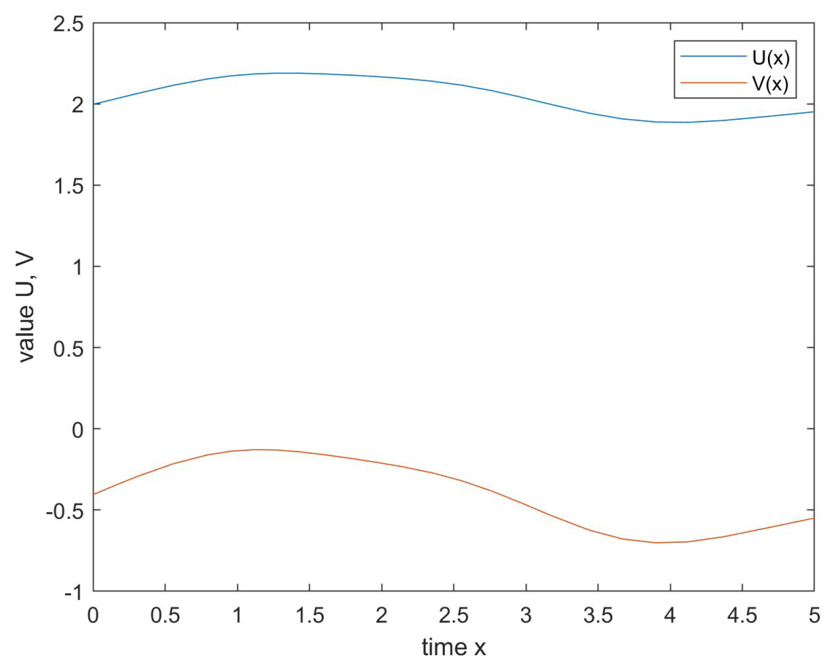
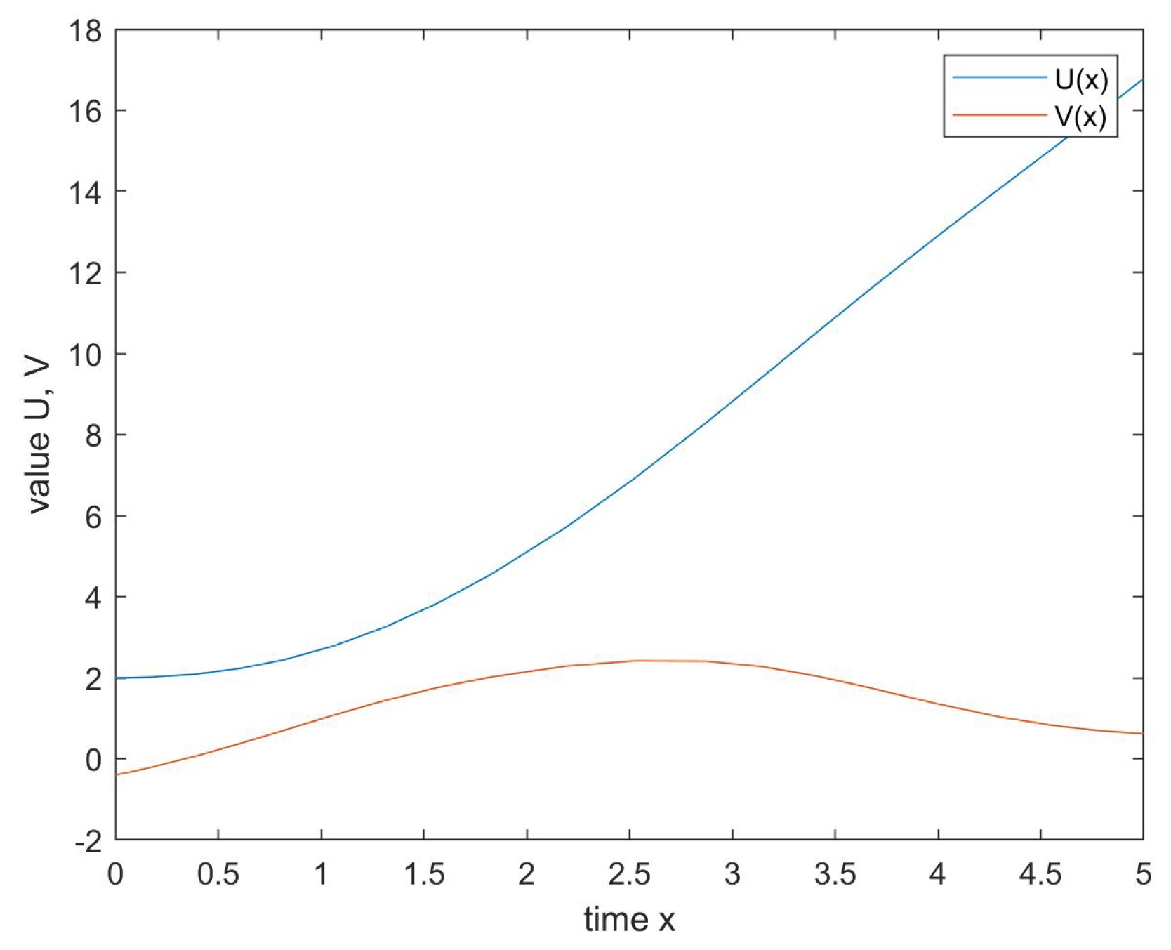
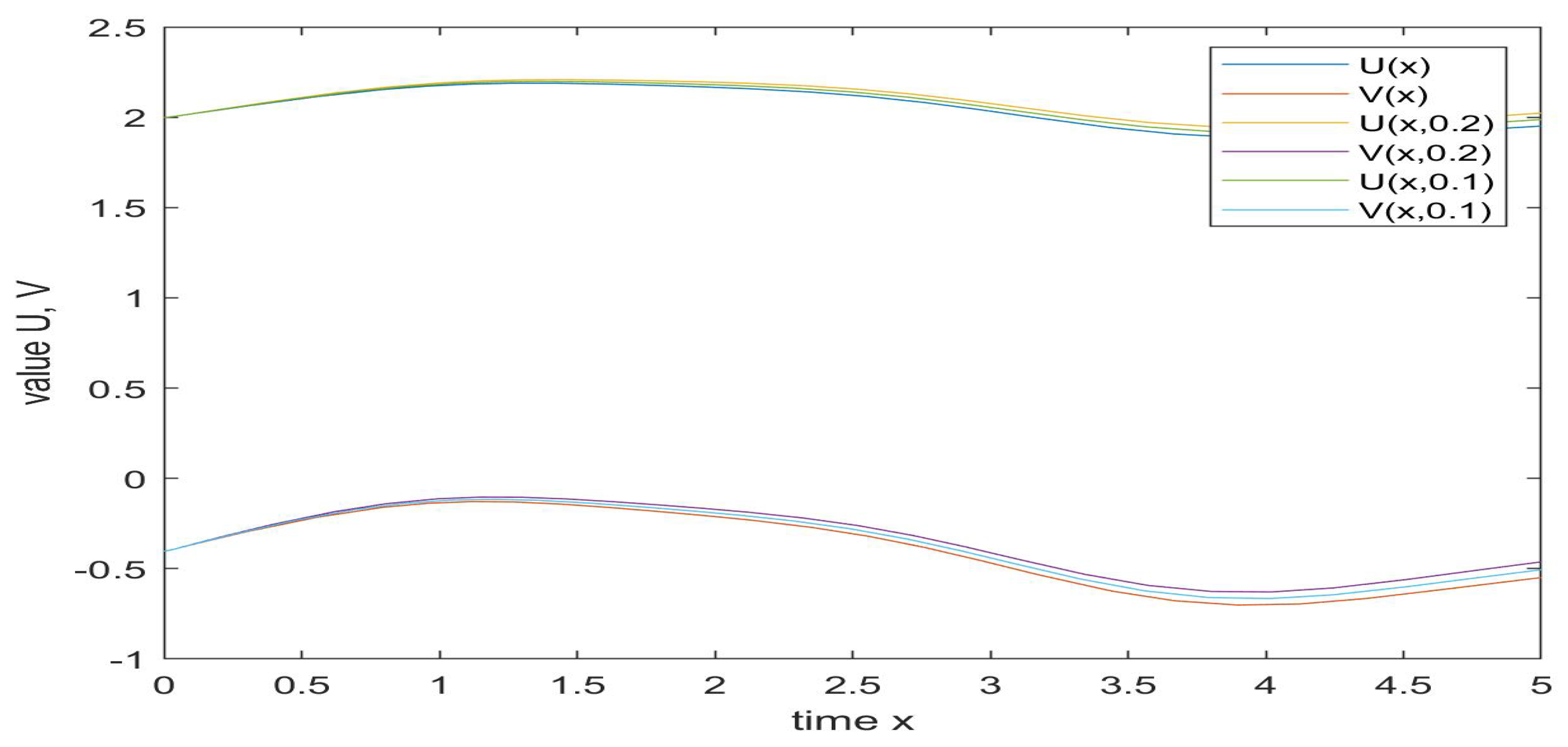
4.2. Numerical Simulation

Let V ( x ) = ( M L D 0 + μ λ ) U ( x ) , then the Equation (1) is transformed into a system of equations as below:
M L D 0 + μ U ( x ) = λ U ( x ) + V ( x ) , x ( 0 , T ] , M L D 0 + ν V ( x ) = f x , ( I 1 U ) ( x ) , ( I 2 U ) ( x ) , x ( 0 , T ] , ( I 1 U ) ( x ) = σ 1 ( x ) 0 k ( s ) U ( x + s ) d s , ( I 2 U ) ( x ) = 0 x U ( s ) d H ( s ) , x J = [ 0 , T ] , U ( x ) = ω 1 ( x ) , V ( x ) = ω 2 ( x ) λ ω 1 ( x ) , x [ σ , 0 ] .
When μ = ν = 1 , the ML-fractional Langevin system (1) is a classical Langevin system formulated by
U ( x ) λ U ( x ) = f x , ( I 1 U ) ( x ) , ( I 2 U ) ( x ) , x ( 0 , T ] , ( I 1 U ) ( x ) = σ 1 ( x ) 0 k ( s ) U ( x + s ) d s , ( I 2 U ) ( x ) = 0 x U ( s ) d H ( s ) , x J = [ 0 , T ] , U ( x ) = ω 1 ( x ) , U ( x ) = ω 2 ( x ) , x [ σ , 0 ] .
Let V ( x ) = ( d d x λ ) U ( x ) , then the Equation (27) is transformed into the following equivalent equations
U ( x ) = λ U ( x ) + V ( x ) , x ( 0 , T ] , V ( x ) = f x , ( I 1 U ) ( x ) , ( I 2 U ) ( x ) , x ( 0 , T ] , ( I 1 U ) ( x ) = σ 1 ( x ) 0 k ( s ) U ( x + s ) d s , ( I 2 U ) ( x ) = 0 x U ( s ) d H ( s ) , x J = [ 0 , T ] , U ( x ) = ω 1 ( x ) , V ( x ) = ω 2 ( x ) λ ω 1 ( x ) , x [ σ , 0 ] .
Next we numerically simulate and discuss the solutions of (25) and the corresponding classical system (27).
Discussion. Under the condition of the same parameter value, the simulations of solutions of (25) and its corresponding classical Langevin system are shown as Figure 1 and Figure 2, respectively. The simulations of UH-stability of (25) is shown as Figure 3. U ( x ) is the solution of Langevin system in all figures. It is easily to see from the figures that the solution of the classical Langevin system is strictly monotonically increasing and increases sharply, while the solution of ML-fractional Langevin system oscillates slightly and is relatively smooth and steady. In contrast, the ML-fractional Langevin system (25) can better reflect the stationarity of Brownian particles in the statistical sense. When 0 < ϵ 1 , the solution curve of the inequality (10) almost coincides with that of system (25), which shows that the system of (25) is HU stable.

5. Conclusions

Some studies show that fractional Langevin equation is more effective than classical Langevin equation in describing the random motion of Brownian particles. To my best knowledge, the current papers on fractional Langevin system are all about RL- or CR-fractional derivatives. However, RL- and CR-fractional derivatives produce singularities under certain conditions, which makes them difficult to be applied to some physical fields. Excitedly, the ML-fractional derivative can overcome this disadvantage. In the paper, we first define an appropriate generalised metric on the continuous function space. Then, we obtain some condition for the existence and uniqueness of solution as well as HUR- and HU-stability for the ML-fractional Langevin system (1) with distributed lag and integral control by using Diaz and Margolis’s fixed-point theorem. Using our main outcomes, an example is theoretically analyzed and numerically simulated. Compared with the numerical simulation of the corresponding classical Langevin system, we find that the fractional Langevin system is more detailed and accurate than the corresponding classical Langevin system in describing the change process of the system. Our findings can provide mathematical theoretical support for some physical problems. Furthermore, the mathematical theories and methods used in this paper can be made use of a reference for the study of other fractional differential system.

Funding

The APC was funded by research start-up funds for high-level talents of Taizhou University.

Institutional Review Board Statement

Not applicable.

Informed Consent Statement

Not applicable.

Data Availability Statement

No data were used to support this study.

Acknowledgments

The author would like to express my heartfelt thanks to the editors and reviewers for their constructive comments.

Conflicts of Interest

The authors declare no conflict of interest.

References

  1. Hilfer, R. Applications of Fractional Calculus in Physics; World Scientific: Singapore, 2000. [Google Scholar]
  2. Beck, C.; Roepstorff, G. From dynamical systems to the langevin equation. Physica A 1987, 145, 1–14. [Google Scholar] [CrossRef]
  3. Coffey, W.; Kalmykov, Y.; Waldron, J. The Langevin Equation; World Scientific: Singapore, 2004. [Google Scholar]
  4. Kubo, R. The fluctuation-dissipation theorem. Rep. Prog. Phys. 1966, 29, 255. [Google Scholar] [CrossRef] [Green Version]
  5. Kubo, R.; Toda, M.; Hashitsume, N. Statistical Physics II; Springer: Berlin, Germany, 1991. [Google Scholar]
  6. Eab, C.; Lim, S. Fractional generalized langevin equation approach to single-file diffusion. Physica A 2010, 389, 2510–2521. [Google Scholar] [CrossRef] [Green Version]
  7. Sandev, T.; Tomovski, Z. Langevin equation for a free particle driven by power law type of noises. Phys. Lett. A 2014, 378, 1–9. [Google Scholar] [CrossRef]
  8. Abbas, M.; Ragusa, M. Solvability of Langevin equations with two Hadamard fractional derivatives via Mittag-Leffler functions. Appl. Anal. 2022, 101, 3231–3245. [Google Scholar] [CrossRef]
  9. Abbas, M. Investigation of Langevin equation in terms of generalized proportional fractional derivatives with respect to another function. Filomat 2021, 35, 4073–4085. [Google Scholar] [CrossRef]
  10. Ulam, S. A Collection of Mathematical Problems-Interscience Tracts in Pure and Applied Mathmatics; Interscience: New York, NY, USA, 1906. [Google Scholar]
  11. Hyers, D. On the stability of the linear functional equation. Proc. Nat. Acad. Sci. USA 1941, 27, 2222–2240. [Google Scholar] [CrossRef] [Green Version]
  12. Rezaei, H.; Jung, S.; Rassias, T. Laplace transform and Hyers-Ulam stability of linear differential equations. J. Math. Anal. Appl. 2013, 403, 244–251. [Google Scholar] [CrossRef]
  13. Wang, C.; Xu, T. Hyers-Ulam stability of fractional linear differential equations involving Caputo fractional derivatives. Appl. Math.-Czech. 2015, 60, 383–393. [Google Scholar] [CrossRef] [Green Version]
  14. Haq, F.; Shah, K.; Rahman, G. Hyers-Ulam stability to a class of fractional differential equations with boundary conditions. Int. J. Appl. Comput. Math. 2017, 3, 1135–1147. [Google Scholar] [CrossRef]
  15. Ibrahim, R. Generalized Ulam-Hyers stability for fractional differential equations. Int. J. Math. 2014, 23, 9. [Google Scholar] [CrossRef] [Green Version]
  16. Yu, X. Existence and β-Ulam-Hyers stability for a class of fractional differential equations with non-instantaneous impulses. Adv. Differ. Equ. 2015, 2015, 104. [Google Scholar] [CrossRef] [Green Version]
  17. Gao, Z.; Yu, X. Stability of nonlocal fractional Langevin differential equations involving fractional integrals. J. Appl. Math. Comput. 2017, 53, 599–611. [Google Scholar] [CrossRef]
  18. Caputo, M.; Fabrizio, M. A new definition of fractional derivative without singular kernel. Progr. Fract. Differ. App. 2015, 1, 73–85. [Google Scholar]
  19. Atangana, A.; Baleanu, D. New fractional derivatives with nonlocal and non-singular kernel: Theory and application to heat transfer model. Therm. Sci. 2016, 20, 763–769. [Google Scholar] [CrossRef] [Green Version]
  20. Sadeghi, S.; Jafari, H.; Nemati, S. Operational matrix for Atangana-Baleanu derivative based on Genocchi polynomials for solving FDEs. Chaos Solit. Fract. 2020, 135, 109736. [Google Scholar] [CrossRef]
  21. Ganji, R.M.; Jafari, H.; Baleanu, D. A new approach for solving multi variable orders differential equations with Mittag-Leffler kernel. Chaos Solit. Fract. 2020, 130, 109405. [Google Scholar] [CrossRef]
  22. Tajadodi, H. A Numerical approach of fractional advection-diffusion equation with Atangana-Baleanu derivative. Chaos Solit. Fract. 2020, 130, 109527. [Google Scholar] [CrossRef]
  23. Khan, H.; Khan, A.; Jarad, F.; Shah, A. Existence and data dependence theorems for solutions of an ABC-fractional order impulsive system. Chaos Solit. Fract. 2020, 131, 109477. [Google Scholar] [CrossRef]
  24. Abbas, M. Nonlinear Atangana-Baleanu fractional differential equations involving the Mittag CLeffler integral operator. Mem. Differ. Equ. Math. 2021, 83, 1–11. [Google Scholar]
  25. Khan, H.; Li, Y.; Khan, A.; Khan, A. Existence of solution for a fractional-order Lotka-Volterra reaction-diffusion model with Mittag-Leffler kernel. Math. Meth. Appl. Sci. 2019, 42, 3377–3387. [Google Scholar] [CrossRef]
  26. Acay, B.; Bas, E.; Abdeljawad, T. Fractional economic models based on market equilibrium in the frame of different type kernels. Chaos Solit. Fract. 2020, 130, 109438. [Google Scholar] [CrossRef]
  27. Khan, A.; Gómez-Aguilar, J.F.; Khan, T.S.; Khan, H. Stability analysis and numerical solutions of fractional order HIV/AIDS model. Chaos Solit. Fract. 2019, 122, 119–128. [Google Scholar] [CrossRef]
  28. Khan, H.; Gómez-Aguilar, J.F.; Alkhazzan, A.; Khan, A. A fractional order HIV-TB coinfection model with nonsingular Mittag-Leffler Law. Math. Method Appl. Sci. 2020, 43, 3786–3806. [Google Scholar] [CrossRef]
  29. Koca, I. Modelling the spread of Ebola virus with Atangana-Baleanu fractional operators. Eur. Phys. J. Plus 2018, 133, 100. [Google Scholar] [CrossRef]
  30. Morales-Delgado, V.F.; Gómez-Aguilar, J.F.; Taneco-Hernández, M.A.; Escobar-Jiménez, R.F.; Olivares-Peregrino, V.H. Mathematical modeling of the smoking dynamics using fractional differential equations with local and nonlocal kernel. J. Nonlinear Sci. Appl. 2018, 11, 1004–1014. [Google Scholar] [CrossRef] [Green Version]
  31. Jarad, F.; Abdeljawad, T.; Hammouch, Z. On a class of ordinary differential equations in the frame of Atangana-Baleanu fractional derivative. Chaos Solit. Fract. 2018, 117, 16–20. [Google Scholar] [CrossRef]
  32. Diaz, J.; Margolis, B. Fixed point theorem of the alternative, for contractions on a generalized complete metric space. Bull. Am. Math. Soc. 1968, 74, 305–309. [Google Scholar] [CrossRef] [Green Version]
  33. Jung, S. A fixed point approach to the stability of differential equations y′ = F(x, y). Bull. Malays. Math. Sci. Soc. 2010, 33, 47–56. [Google Scholar]
Figure 1. Solutions of (25).
Axioms 11 00350 g001
Figure 2. Solutions of the classical system (27) corresponding to (25).
Axioms 11 00350 g002
Figure 3. UH-stability of (25) with ϵ = 0 , 0.1 , 0.2 .
Axioms 11 00350 g003
Publisher’s Note: MDPI stays neutral with regard to jurisdictional claims in published maps and institutional affiliations.

