Temporal Cox Process with Folded Normal Intensity

Abstract

In this work, the case of a Cox Process with Folded Normal Intensity (CP-FNI), in which the intensity is given by $\mathrm{\Lambda }\left(t\right)=\left|Z\right(t\left)\right|$, where $Z\left(t\right)$ is a stationary Gaussian process, is studied. Here, two particular cases are dealt with: (i) when the process $Z\left(t\right)$ constitutes a family of independent random variables and with a common probability law $\mathrm{N}(0,1)$, and (ii) the case in which $Z\left(t\right)$ is a second order stationary process, with exponential type covariance function. In these cases, we observe that the properties of the Gaussian process $Z\left(t\right)$ are naturally transferred to the intensity $\mathrm{\Lambda }\left(t\right)$ and that very analytical results are achievable from the analytical point of view for the point process $N\left(t\right)$. Finally, some simulations are presented in order to appreciate what type of counting phenomena can be modeled by these cases of CP-FNI. In particular, it is interesting to see how the trajectories show a tendency of the events to be grouped in certain periods of time, also leaving long periods of time without the occurrence of events.

1. Introduction

The Cox processes provide a wide range of options for the modeling of specific processes over time. Cox [1] presents the case of a point process, which is defined as an extension of the Poisson process, widely studied in the literature, for example, by Ross [2], Barry [3], Cox and Miller [4], Parzen [5] and Rozanov [6], and Daley and Vere-Jones [7], among others. The main characteristic of this process is that it is a point process where the intensity is a stochastic process, such that conditional on each accomplishment or trajectory of it. The specific process is a non-homogeneous Poisson Process with intensity given precisely for this.

Møller et al. [8] introduced the class of Log-Gaussian Processes, where for each $t\ge 0$, $\mathrm{\Lambda }\left(t\right)=e^{Z\left(t\right)}$, being $\left\{Z\right(t):t\ge 0\}$ a Gaussian process. In this case, $\mathrm{\Lambda }\left(t\right)$ follows a Log-Gaussian law, with the parameters corresponding to the Gaussian law of $Z\left(t\right)$, that is, the link function $g\left(z\right)=e^z$ is used to obtain a process of positive values from a Gaussian process. Using this kind of process, several extensions have been proposed. Diggle et al. [9] extend the Cox process with Log-Gaussian intensity process to the spatial domain, and Cuevas-Pacheco and Møller [10] introduce the Log Gaussian Cox processes on the sphere. A generalization of Gaussian Cox process to model multiple correlated point data is provided by Aglietti [11] where closed-form expressions for the moments of the intensity functions are derived. A multivariate version of log-Gaussian Cox processes is also proposed by Waagepetersen et al. [12]. Frías et al. [13] introduce a new class of spatial Cox processes driven by a Hilbert-valued random log-intensity. The log Normal Cox process and its extensions were used in a variety of applications (see, for example, [14,15,16,17]).

Recently, Walder and Bishop [18] proposed the Cox process with Gamma intensity, making a construction analogous to that carried out by [8], but changing the link function that allows obtaining a positive process from a Gaussian process. In particular, they consider $\mathrm{\Lambda }\left(t\right)={\displaystyle \frac{1}{2}}·Z^2\left(t\right)$, which for $t\ge 0$, $\mathrm{\Lambda }\left(t\right)$ follows a Gamma distribution and $\left\{Z\right(t):t\ge 0\}$ is a Gaussian process. This case is also mentioned by Møller et al. [8] for the particular case of a process of mean equal to 0, obtaining the Cox process with Chi-Square intensity (as a particular case of Gamma). The properties of the link function $g\left(z\right)=\frac{1}{2}{z}^2$ are widely studied by Flaxman and Sejdinovic [19]. On the other hand, Adams et al. [20] study a link function given by $g\left(z\right)={\lambda }^{*}{\left(1+e^{-z}\right)}^{-1}.$

In this work we are interested to study positive link functions of the type $g:\mathbb{R}\to {\mathbb{R}}^{+}$, which allow us to obtain a process of positive values from a Gaussian process. In the context of distributions with positive support, Leone et al. [21] proposed the Folded-Normal law or distribution, which it is constructed assuming that $Y=\left|X\right|\sim \mathrm{F}\mathrm{N}(\mu ,{\sigma }^2)$, where $X\sim \mathrm{N}(\mu ,{\sigma }^2)$. A particular case of this distribution is the Half-Normal distribution, which is obtained when $\mu =0$, and is defined as $Y=\left|X\right|\sim \mathrm{H}\mathrm{N}\left({\sigma }^2\right)$, with $X\sim \mathrm{N}(0,{\sigma }^2)$. Thus, $Y\sim \mathrm{F}\mathrm{N}(0,{\sigma }^2)\iff Y\sim \mathrm{H}\mathrm{N}\left({\sigma }^2\right)$. The properties of this law of probability are widely studied by Tsagris et al. [22]. In this same guideline, Psarakis and Panaretos [23] proposed an extension of the Folded Gaussian to the bivariate case and considering the Folded $t-$ distribution, while Chakraborty and Chatterjee [24], and Kan and Robotti [25] studied the properties of the multivariate Folded Gaussian distribution. Different other folded models are described in Nadarajah and Bakar [26] where the Folded Normal distribution and the Folded Laplace distribution (introduced by Liu and Kozubowski [27]) are particular cases of the exponential power distribution presented by Subbotin [28]. Additionally, Chatterjee and Chakraborty [29] proposed a simple procedure for calculating the values of a Folded Normal distribution, and Liu et al. [30] presented a new ML algorithm for estimating the parameters of a Folded Normal distribution and a Folded Normal regression model.

In this work we propose the Cox process with Folded Normal intensity process (CP-FNI) and study some of its characteristics and properties. This paper is organized as follows. In Section 2, the Folded Normal Intensity process is described. In Section 3, the Cox Process with Folded Normal Intensity (CP-NFI) and its properties are introduced. A simulation study is provided in Section 4. Finally, conclusions and future work are described in Section 5.

2. The Folded Normal Intensity Process

In this section, the Folded Normal Intensity Process and some numerical features such as the mean, variance and covariance functions, are defined.

2.1. Definition

Let $\left\{Z\right(t):t\ge 0\}$ a Gaussian Process such that for each collection of times $t_1<t_2<\dots <t_n$ it is verified that

$$\left(\begin{array}{c}Z\left(t_1\right)\\ ⋮\\ Z\left(t_n\right)\end{array}\right)\sim {\mathrm{N}}_n\left(\mathit{\mu },\mathsf{\Sigma }\right),$$

(1)

where $\mathit{\mu }={(\mu ,\dots ,\mu )}^T$ denotes the vector of the means and $\mathsf{\Sigma }=\left({\sigma }_{ij}\right)$ the matrix of the variance and covariance, with ${\sigma }_{ij}=k_Z(t_i-t_j)=k_Z\left(h\right)$, $h=|t_i-t_j|$ and $k_Z\left(0\right)={\sigma }^2$. Due to the need to model random phenomena involving positive data, functions are required to generate data with such a characteristic from a given intensity process. A type of link function that allows us to define positive values from a Gaussian process is given by

$$\begin{array}{ccc}\hfill g:\mathbb{R}& \to & {\mathbb{R}}^{+}\hfill \\ \hfill z& \mapsto & g\left(z\right).\hfill \end{array}$$

This type of link is called a positive link. If we consider $g\left(z\right)=\left|z\right|$, the intensity process $\{\mathrm{\Lambda }(t):t\ge 0\}$ can be defined in the form

$$\mathrm{\Lambda }\left(t\right)=\left|Z\right(t\left)\right|,$$

(2)

for $t\ge 0$. It can be shown that $\mathrm{\Lambda }\left(t\right)$ follows a Folded Normal (FN) law. This result is established in the following subsection.

2.2. Properties

Next, some results related to certain numerical characteristics of the intensity process $\{\mathrm{\Lambda }(t):t\ge 0\}$ are presented. Specifically, the mean, variance and covariance function are derived.

Proposition 1.

Let $\{\mathrm{\Lambda }(t):t\ge 0\}$ be an intensity process. Then,

$$\mathrm{\Lambda }\left(t\right)\sim FN(\mu ,{\sigma }^2).$$

(3)

Proof. 

From Equation (1), it is immediate that, for all t, $Z\left(t\right)\sim \mathrm{N}(\mu ,{\sigma }^2)$. Furthermore, from the definition of the law of the process, proposed in Equation (2), the proof is completed.

□

Proposition 2.

The intensity process $\{\mathrm{\Lambda }(t):t\ge 0\}$ is such that:

(a)

(mean value function)

$$m_{\mathrm{\Lambda }}\left(t\right)=\sqrt{{\displaystyle \frac{2}{\pi }}}\sigma ·e^{-\frac{{\mu }^2}{2{\sigma }^2}}+\mu ·\left[1-2\mathsf{\Phi }\left(-{\displaystyle \frac{\mu }{\sigma }}\right)\right];$$

(4)

(b)

(variance value function)

$$v_{\mathrm{\Lambda }}\left(t\right)={\mu }^2+{\sigma }^2-{\left\{\sqrt{{\displaystyle \frac{2}{\pi }}}\sigma ·e^{-\frac{{\mu }^2}{2{\sigma }^2}}+\mu ·\left[1-2\mathsf{\Phi }\left(-{\displaystyle \frac{\mu }{\sigma }}\right)\right]\right\}}^2,$$

(5)

where, in both cases, $\mathsf{\Phi }(·)$ denotes the distribution function of a random variable with standard normal distribution.

Proof. 

It is immediate of the Proposition 1 and the results presented by Tsagris et al. [22].

□

Proposition 3.

The intensity process $\{\mathrm{\Lambda }(t):t\ge 0\}$, for the particular case in which $\mu =0$, satisfies

$$k_{\mathrm{\Lambda }}(t,s)=\mathbf{C}\left[\mathrm{\Lambda }\left(t\right),\mathrm{\Lambda }\left(s\right)\right]={\displaystyle \frac{2}{\pi }}\left[\sqrt{{\sigma }^4-k_Z^2(t-s)}+k_Z(t-s)·arcsin{\displaystyle \frac{k_Z(t-s)}{{\sigma }^2}}-{\sigma }^2\right].$$

Proof. 

For the case $\mu =0$, we have that $\mathrm{\Lambda }\left(t\right)\sim \mathrm{H}\mathrm{N}\left({\sigma }^2\right)$ and as an immediate consequence of Proposition 2, $\mathbb{E}[\mathrm{\Lambda }\left(t\right)]=\sqrt{{\displaystyle \frac{2}{\pi }}}\sigma$. On the other hand, from the fact that $\mathrm{\Lambda }\left(t\right)=\left|Z\right(t\left)\right|$, we obtain that

$$\begin{array}{ccc}\hfill k_{\mathrm{\Lambda }}(t,s)& =& \mathbf{C}\left[\mathrm{\Lambda }\left(t\right),\mathrm{\Lambda }\left(s\right)\right]\hfill \\ & =& \mathbf{C}\left(\left|Z\right(t\left)\right|,\left|Z\right(s\left)\right|\right)\hfill \\ & =& \mathbb{E}\left[\left|Z\right(t\left)\right|·\left|Z\right(s\left)\right|\right]-\mathbb{E}\left[\left|Z\right(t\left)\right|\right]·\mathbb{E}\left[\left|Z\right(s\left)\right|\right]\hfill \\ & =& \mathbb{E}\left[\left|Z\right(t)·Z(s\left)\right|\right]-{\left\{\sqrt{{\displaystyle \frac{2}{\pi }}}\sigma \right\}}^2.\hfill \end{array}$$

Now, we consider the fact that if ${\left(Y_1{Y}_2\right)}^T$ is a Gaussian random vector with mean vector ${\left(00\right)}^T$, $\mathbb{E}\left(Y_1^2\right)={\sigma }_1^2$, $\mathbb{E}\left(Y_2^2\right)={\sigma }_2^2$, and $\mathbb{E}\left(Y_1{Y}_2\right)=\rho {\sigma }_1{\sigma }_2$, then

$$\mathbb{E}\left[|Y_1{Y}_2|\right]={\displaystyle \frac{2{\sigma }_1{\sigma }_2}{\pi }}\left(\sqrt{1-{\rho }^2}+\rho ·arcsin\rho \right).$$

The demonstration can be found in Li and Wei [31]. Based on this result and considering $\mathbb{E}\left[Z\right(t\left)\right]=0$ and $\mathbb{V}\left[Z\left(t\right)\right]={\sigma }^2$, for all $t\ge 0$, then

$$\begin{array}{ccc}\hfill \mathbb{E}\left[\left|Z\right(t)·Z(s\left)\right|\right]& =& {\displaystyle \frac{2{\sigma }^2}{\pi }}\left[\sqrt{1-{\left({\displaystyle \frac{k_Z(t-s)}{{\sigma }^2}}\right)}^2}+{\displaystyle \frac{k_Z(t-s)}{{\sigma }^2}}·\arcsin {\displaystyle \frac{k_Z(t-s)}{{\sigma }^2}}\right]\hfill \\ & =& {\displaystyle \frac{2{\sigma }^2}{\pi }}\left[\sqrt{{\displaystyle \frac{{\sigma }^4-k_Z^2(t-s)}{{\sigma }^4}}}+{\displaystyle \frac{k_Z(t-s)}{{\sigma }^2}}·\arcsin {\displaystyle \frac{k_Z(t-s)}{{\sigma }^2}}\right]\hfill \\ & =& {\displaystyle \frac{2}{\pi }}\left[\sqrt{{\sigma }^4-k_Z^2(t-s)}+k_Z(t-s)·\arcsin {\displaystyle \frac{k_Z(t-s)}{{\sigma }^2}}\right]\hfill \end{array}$$

Consequently,

$$\begin{array}{ccc}\hfill k_{\mathrm{\Lambda }}(t,s)& =& {\displaystyle \frac{2}{\pi }}\left[\sqrt{{\sigma }^4-k_Z^2(t-s)}+k_Z(t-s)·\arcsin {\displaystyle \frac{k_Z(t-s)}{{\sigma }^2}}\right]-{\left\{\sqrt{{\displaystyle \frac{2}{\pi }}}\sigma \right\}}^2\hfill \\ & =& {\displaystyle \frac{2}{\pi }}\left[\sqrt{{\sigma }^4-k_Z^2(t-s)}+k_Z(t-s)·\arcsin {\displaystyle \frac{k_Z(t-s)}{{\sigma }^2}}\right]-{\displaystyle \frac{2{\sigma }^2}{\pi }}\hfill \\ & =& {\displaystyle \frac{2}{\pi }}\left[\sqrt{{\sigma }^4-k_Z^2(t-s)}+k_Z(t-s)·\arcsin {\displaystyle \frac{k_Z(t-s)}{{\sigma }^2}}-{\sigma }^2\right]\hfill \end{array}$$

As we wanted to show.

□

Remark 1.

Note that, from the Propositions 2 and 3, it is immediate that for the case $\mu =0$ the intensity process $\{\mathrm{\Lambda }(t):t\ge 0\}$ is a second order stationary process. In particular, if we make $t-s=h$ and choose the covariance function

$$k_Z\left(h\right)={\sigma }^2·e^{-\beta \left|h\right|},h\in \mathbb{R},$$

we have

$$k_{\mathrm{\Lambda }}\left(h\right)={\displaystyle \frac{2{\sigma }^2}{\pi }}\left[\sqrt{1-e^{-2\beta \left|h\right|}}+e^{-\beta \left|h\right|}·\arcsin e^{-\beta \left|h\right|}-1\right].$$

(6)

This is the first particular case that is studied in this work.

Proposition 4.

The intensity process $\{\mathrm{\Lambda }(t):t\ge 0\}$, for the particular case in which

$$k_Z(t,s)=\left\{\begin{array}{cc}{\sigma }^2\hfill & t=s\hfill \\ 0\hfill & t\ne s,\hfill \end{array}\right.$$

satisfies

$$k_{\mathrm{\Lambda }}(t,s)=\left\{\begin{array}{cc}{\mu }^2+{\sigma }^2-{\left\{\sqrt{{\displaystyle \frac{2}{\pi }}}\sigma ·e^{-\frac{{\mu }^2}{2{\sigma }^2}}+\mu ·\left[1-2\mathsf{\Phi }\left(-{\displaystyle \frac{\mu }{\sigma }}\right)\right]\right\}}^2\hfill & t=s\hfill \\ 0\hfill & t\ne s.\hfill \end{array}\right.$$

Proof. 

First, note that for the function of covariance $k_Z$, we have that the process $\left\{Z\right(t):t\ge 0\}$ is a family of independent variables with a common distribution $\mathrm{N}(\mu ,{\sigma }^2)$. On the other hand, since $k_Z(t,s)=\mathbf{C}[Z\left(t\right),Z\left(s\right)]=0$ if $t\ne s$, it follows that $Z\left(t\right)\perp Z\left(s\right)$ for each $t\ne s$. Second, from hereditary property of independence, discussed for example in [3], which states that if $U\perp V$ and f is a measurable function, then $f\left(U\right)\perp f\left(V\right)$, we conclude that, for $f(·)=|·|$,

$$\begin{array}{ccc}\hfill t\ne s& \Rightarrow & Z\left(t\right)\perp Z\left(s\right)\hfill \\ & \Rightarrow & \left|Z\right(t\left)\right|\perp \left|Z\right(s\left)\right|\hfill \\ & \Rightarrow & \mathrm{\Lambda }\left(t\right)\perp \mathrm{\Lambda }\left(s\right).\hfill \end{array}$$

Hence, it is immediate that $k_{\mathrm{\Lambda }}(t,s)=0$ when $t\ne s$. Finally, for the case $t=s$

$$\begin{array}{ccc}\hfill k_{\mathrm{\Lambda }}(t,s)& =& k_{\mathrm{\Lambda }}(t,t)\hfill \\ & =& \mathbf{C}[\mathrm{\Lambda }(t),\mathrm{\Lambda }(t\left)\right]\hfill \\ & =& \mathbb{V}[\mathrm{\Lambda }(t\left)\right]\hfill \\ & =& {\mu }^2+{\sigma }^2-{\left\{\sqrt{{\displaystyle \frac{2}{\pi }}}\sigma ·e^{-\frac{{\mu }^2}{2{\sigma }^2}}+\mu ·\left[1-2\mathsf{\Phi }\left(-{\displaystyle \frac{\mu }{\sigma }}\right)\right]\right\}}^2,\hfill \end{array}$$

where the last equation is obtained directly from the Proposition 2.

□

Remark 2.

From the Propositions 2 and 4, it is immediate that for the case $k_Z(t,s)={\sigma }^2·I_{\{t=s\}}$, where $I_A$ denotes the indicator function, the intensity process $\{\mathrm{\Lambda }(t):t\ge 0\}$ is a second order stationary process, moreover, it is even strictly stationary. In particular, if we do $t-s=h$, this can be written as $k_Z\left(h\right)={\sigma }^2·I_{\left\{0\right\}}\left(h\right)$ and the covariance function of the intensity process is reduced simply to

$$k_{\mathrm{\Lambda }}\left(h\right)=\left({\mu }^2+{\sigma }^2-{\left\{\sqrt{{\displaystyle \frac{2}{\pi }}}\sigma ·e^{-\frac{{\mu }^2}{2{\sigma }^2}}+\mu ·\left[1-2\mathsf{\Phi }\left(-{\displaystyle \frac{\mu }{\sigma }}\right)\right]\right\}}^2\right)·I_{\left\{0\right\}}\left(h\right)$$

(7)

This is the second particular case that is studied in this work.

Remark 3.

It is important to mention that we can obtain a point process $\left\{N\right(t):t\ge 0\}$, which is a Cox Process with Folded Normal Intensity (CP-NFI) defined by (1), (2) and (3).

3. Properties of the CP-NFI

In this section, the density function associated with the process CP-NFI is presented, and its first and second moments are derived.

3.1. Process Density

For the process $\left\{N\right(t):t\ge 0\}$ it is verified that

$$\mathbb{P}\left(N\left(t\right)=n\right)=\mathbb{E}\left[\mathbb{P}\left(N\left(t\right)=n|\mathrm{\Lambda }(t)\right)\right].$$

(8)

Now, doing

$${\displaystyle M\left(t\right)={\int }_0^t\mathrm{\Lambda }\left(s\right)ds}$$

(9)

and using the fact that, conditional to any path of the intensity process $\{\mathrm{\Lambda }(t):t\ge 0\}$, the process $\left\{N\right(t):t\ge 0\}$ is an inhomogenous Poisson Process, we have:

$$\mathbb{P}\left(N\left(t\right)=n\right)=\mathbb{E}\left[{\displaystyle \frac{{\left[M\left(t\right)\right]}^n{e}^{-M\left(t\right)}}{n!}}\right].$$

(10)

In our particular case, the Equation (9) can be written as

$${\displaystyle M\left(t\right)={\int }_0^t\left|Z\left(s\right)\right|ds,}$$

(11)

where $\left\{Z\right(s):s\ge 0\}$ corresponds to one of the two Gaussian process we have considered to construct the Folded Normal intensity process; that is, in cases where $\left\{Z\right(s):s\ge 0\}$ corresponds to a family of independent variables with a common law $\mathrm{N}(\mu ,{\sigma }^2)$, or in which $\left\{Z\right(s):s\ge 0\}$ is a stationary Gaussian process with mean equal to zero and covariance function $k_Z\left(h\right)={\sigma }^2{e}^{-\beta \left|h\right|}$. Hence, Equation (10) can be rewritten as

$$\mathbb{P}\left(N\left(t\right)=n\right)={\displaystyle \frac{1}{n!}}·\mathbb{E}\left[{\left({\displaystyle {\int }_0^t\left|Z\left(s\right)\right|ds}\right)}^n·exp\left({\displaystyle -{\int }_0^t\left|Z\left(s\right)\right|ds}\right)\right].$$

(12)

Following Parzen [5], we can define the integral of the Equation (12) as

$${\displaystyle M\left(t\right)={\int }_0^t\left|Z\left(s\right)\right|ds=\underset{{\displaystyle \underset{k=1\dots n}{max}(t_k-t_{k-1})\to 0}}{lim}\sum _{k=1}^n\left|Z\left(t_k\right)\right|·(t_k-t_{k-1}),}$$

(13)

where the considered limit is, in this case, a limit in quadratic mean. In particular, we can choose an equation such that $t_k-t_{k-1}={\Delta }_n$ be constant in k, but depend on n, and define

$${\displaystyle M\left(t\right)={\int }_0^t\left|Z\left(s\right)\right|ds=\underset{n\to +\infty }{lim}\sum _{k=1}^n\left|Z\left(t_k\right)\right|·{\Delta }_n,}$$

(14)

considering again the limit taken as a limit in quadratic mean.

3.2. Properties of the Process

Note that Equation (9) can be written as

$${\displaystyle M\left(\right]0,t\left]\right)={\int }_{]0,t]}\mathrm{\Lambda }\left(s\right)ds}$$

(15)

and, more generally, for $A\subset {\mathbb{R}}^{+}$, we can write

$${\displaystyle M\left(A\right)={\int }_A\mathrm{\Lambda }\left(s\right)ds.}$$

(16)

According to Møller et al. [32], for bounded intervals $A,B\subset {\mathbb{R}}^{+}$, they are verified the following relationships:

• For the mean of $\left\{N\right(t):t\ge 0\}$ over $A\subset {\mathbb{R}}^{+}$:

  $$\mathbb{E}\left[N\right(A\left)\right]=\mathbb{E}\left[M\right(A\left)\right];$$

  (17)
• For the variance of $\left\{N\right(t):t\ge 0\}$ over $A\subset {\mathbb{R}}^{+}$:

  $$\mathbb{V}\left[N\right(A\left)\right]=\mathbb{V}\left[M\right(A\left)\right]+\mathbb{E}\left[M\right(A\left)\right];$$

  (18)
• For the covariance of $\left\{N\right(t):t\ge 0\}$ over $A,B\subset {\mathbb{R}}^{+}$:

  $$\mathbf{C}\left[N\right(A),N(B\left)\right]=\mathbf{C}\left[M\right(A),M(B\left)\right]+\mathbb{E}\left[M\right(A\cap B\left)\right].$$

  (19)

Proposition 5.

The process CP-NFI satisfies the following properties:

(a)

(mean value function)

$$m_N\left(t\right)=\mathbb{E}\left[{\displaystyle {\int }_0^t\left|Z\left(u\right)\right|du}\right];$$

(20)

(b)

(variance value function)

$$v_N\left(t\right)=\mathbb{V}\left[{\displaystyle {\int }_0^t\left|Z\left(u\right)\right|du}\right]+\mathbb{E}\left[{\displaystyle {\int }_0^t\left|Z\left(u\right)\right|du}\right];$$

(21)

(c)

(covariance value function)

$$k_N(t,s)=\mathbf{C}\left[{\displaystyle {\int }_0^t\left|Z\left(u\right)\right|du,{\int }_0^t\left|Z\left(v\right)\right|dv}\right]+\mathbb{E}\left[{\displaystyle {\int }_0^{min\{s,t\}}\left|Z\left(u\right)\right|du}\right].$$

(22)

Proof. 

In this case, the proof is direct, since Equations (17)–(19) can be written in terms of the interval $]0,t]$. Then, considering Equation (15), the integral given by (11) and the fact that $]0,t]\cap ]0,s]=]0,min\{t,s\left\}\right]$, the proof is complete. □

Remark 4.

Note that, from Equation (9), the results of Proposition 5 can be directly expressed in terms of the intensity process $\{\mathrm{\Lambda }(t):t\ge 0\}$, as

(a’)

$m_N\left(t\right)=\mathbb{E}\left[{\displaystyle {\int }_0^t\mathrm{\Lambda }\left(u\right)du}\right]$;

(b’)

$v_N\left(t\right)=\mathbb{V}\left[{\displaystyle {\int }_0^t\mathrm{\Lambda }\left(u\right)du}\right]+\mathbb{E}\left[{\displaystyle {\int }_0^t\mathrm{\Lambda }\left(u\right)du}\right]$;

(c’)

$k_N(t,s)=\mathbf{C}\left[{\displaystyle {\int }_0^t\mathrm{\Lambda }\left(u\right)du,{\int }_0^s\mathrm{\Lambda }\left(v\right)dv}\right]+\mathbb{E}\left[{\displaystyle {\int }_0^{min\{s,t\}}\mathrm{\Lambda }\left(u\right)du}\right]$.

Proposition 6.

The process CP-NFI based on a Gaussian process with average value function $m_Z\left(t\right)=0$ and with covariance function $k_Z(t,s)={\sigma }^2{e}^{-\beta |t-s|}$ satisfies the following properties:

(a)

(mean value function)

$$m_N\left(t\right)=\sqrt{{\displaystyle \frac{2}{\pi }}}\sigma t;$$

(23)

(b)

(variance value function)

$$v_N\left(t\right)=D\left(t\right)+{\displaystyle \frac{2{\sigma }^2{t}^2}{\pi }}+\sqrt{{\displaystyle \frac{2}{\pi }}}\sigma t,$$

(24)

with

$${\displaystyle D\left(t\right)={\displaystyle \frac{2{\sigma }^2}{\pi }}{\int }_0^t{\int }_0^t\left[\sqrt{1-e^{-2\beta |u-s|}}+e^{-\beta |u-s|}·\arcsin e^{-\beta |u-s|}\right]duds;}$$

(25)

(c)

(covariance value function)

$$k_N(t,s)=B(t,s)+{\displaystyle \frac{2{\sigma }^2{t}^2}{\pi }}+\sqrt{{\displaystyle \frac{2}{\pi }}}\sigma min\{s,t\},$$

(26)

with

$${\displaystyle B(t,s)={\displaystyle \frac{2{\sigma }^2}{\pi }}{\int }_0^t{\int }_0^s\left[\sqrt{1-e^{-2\beta |u-v|}}+e^{-\beta |u-s|}·\arcsin e^{-\beta |u-v|}\right]dvdu.}$$

(27)

Proof. 

First, consider the following result described by Parzen [5] and Loéve [33]: let $\left\{X\right(t):t\ge 0\}$ be a stochastic process of continuous parameter with finite second order moments, whose functions of average value $m_X$ and covariance $k_X$ are continuous functions. Consequently, we have:

(i)

${\displaystyle {\int }_a^{b}X\left(t\right)dt}$, defined in the Equation (13), is well defined;

(ii)

${\displaystyle \mathbb{E}\left[{\displaystyle {\int }_a^{b}X\left(t\right)dt}\right]={\int }_a^b{m}_X\left(t\right)dt}$;

(iii)

${\displaystyle \mathbb{V}\left[{\displaystyle {\int }_a^{b}X\left(t\right)dt}\right]={\int }_a^b{\int }_a^b{k}_X(t,s)dtds=2{\int }_a^b{\int }_a^t{k}_X(t,s)dsdt}$;

(iv)

${\displaystyle \mathbf{C}\left[{\displaystyle {\int }_a^{b}X\left(t\right)dt,{\int }_c^{d}X\left(s\right)ds}\right]={\int }_a^b{\int }_c^d{k}_X(t,s)dsdt}$.

Consider Proposition 2 for $\mu$ = 0 and the expectation operator given in ($ii$). Then, the process mean value function is given by

$$\begin{array}{ccc}\hfill m_N\left(t\right)& =& \mathbb{E}\left[{\displaystyle {\int }_0^t\mathrm{\Lambda }\left(u\right)du}\right]\hfill \\ & =& {\displaystyle {\int }_0^t{m}_{\mathrm{\Lambda }}\left(s\right)ds}\hfill \\ & =& {\displaystyle {\int }_0^t\sqrt{{\displaystyle \frac{2}{\pi }}}\sigma ds}\hfill \\ & =& \sqrt{{\displaystyle \frac{2}{\pi }}}\sigma t.\hfill \end{array}$$

On the other hand, considering Proposition 3, the result ($iii$) and mean value function obtained previously, the function of the variance value takes the form

$$\begin{array}{ccc}\hfill v_N\left(t\right)& =& \mathbb{V}\left[{\displaystyle {\int }_0^t\mathrm{\Lambda }\left(u\right)du}\right]+\mathbb{E}\left[{\displaystyle {\int }_0^t\mathrm{\Lambda }\left(u\right)du}\right]\hfill \\ & =& {\displaystyle {\int }_0^t{\int }_0^t{k}_{\mathrm{\Lambda }}(u,s)duds+\sqrt{{\displaystyle \frac{2}{\pi }}}\sigma t}\hfill \\ & =& {\displaystyle {\int }_0^t{\int }_0^t{\displaystyle \frac{2{\sigma }^2}{\pi }}\left[\sqrt{1-e^{-2\beta |u-s|}}+e^{-\beta |u-s|}·\arcsin e^{-\beta |u-s|}-1\right]duds+\sqrt{{\displaystyle \frac{2}{\pi }}}\sigma t}\hfill \\ & =& {\displaystyle {\displaystyle \frac{2{\sigma }^2}{\pi }}{\int }_0^t{\int }_0^t\left[\sqrt{1-e^{-2\beta |u-s|}}+e^{-\beta |u-s|}·\arcsin e^{-\beta |u-s|}\right]duds}\hfill \\ & & +{\displaystyle \frac{2{\sigma }^2{t}^2}{\pi }}+\sqrt{{\displaystyle \frac{2}{\pi }}}\sigma t\hfill \\ & =& D\left(t\right)+{\displaystyle \frac{2{\sigma }^2{t}^2}{\pi }}+\sqrt{{\displaystyle \frac{2}{\pi }}}\sigma t,\hfill \end{array}$$

with

$${\displaystyle D\left(t\right)={\displaystyle \frac{2{\sigma }^2}{\pi }}{\int }_0^t{\int }_0^t\left[\sqrt{1-e^{-2\beta |u-s|}}+e^{-\beta |u-s|}·\arcsin e^{-\beta |u-s|}\right]duds.}$$

Finally, by considering Proposition 3 again and the mean value function obtained in this proposition, the covariance function is given by

$$\begin{array}{ccc}\hfill k_N(t,s)& =& \mathbf{C}\left[{\displaystyle {\int }_0^t\mathrm{\Lambda }\left(u\right)du,{\int }_0^s\mathrm{\Lambda }\left(v\right)dv}\right]+\mathbb{E}\left[{\displaystyle {\int }_0^{min\{s,t\}}\mathrm{\Lambda }\left(u\right)du}\right]\hfill \\ & =& {\displaystyle {\int }_0^t{\int }_0^s{k}_{\mathrm{\Lambda }}(u,v)dvdu+\sqrt{{\displaystyle \frac{2}{\pi }}}\sigma min\{s,t\}}\hfill \\ & =& {\displaystyle {\int }_0^t{\int }_0^s{\displaystyle \frac{2{\sigma }^2}{\pi }}\left[\sqrt{1-e^{-2\beta |u-v|}}+e^{-\beta |u-v|}·\arcsin e^{-\beta |u-v|}-1\right]dvdu}\hfill \\ & & +\sqrt{{\displaystyle \frac{2}{\pi }}}\sigma min\{s,t\}\hfill \\ & =& {\displaystyle {\displaystyle \frac{2{\sigma }^2}{\pi }}{\int }_0^t{\int }_0^t\left[\sqrt{1-e^{-2\beta |u-v|}}+e^{-\beta |u-v|}·\arcsin e^{-\beta |u-v|}\right]dvdu}\hfill \\ & & +{\displaystyle \frac{2{\sigma }^{2}ts}{\pi }}+\sqrt{{\displaystyle \frac{2}{\pi }}}\sigma min\{s,t\}\hfill \\ & =& B(t,s)+{\displaystyle \frac{2{\sigma }^2{t}^2}{\pi }}+\sqrt{{\displaystyle \frac{2}{\pi }}}\sigma min\{s,t\},\hfill \end{array}$$

with

$${\displaystyle B(t,s)={\displaystyle \frac{2{\sigma }^2}{\pi }}{\int }_0^t{\int }_0^s\left[\sqrt{1-e^{-2\beta |u-v|}}+e^{-\beta |u-s|}·\arcsin e^{-\beta |u-v|}\right]dvdu.}$$

Thus, the proof is completed.

□

Remark 5.

Naturally, the resolution of $D\left(t\right)$ and $B(t,s)$ presented in the Proposition 6 can be approached by numerical methods. In the literature there is a wide discussion about how to approximate integrals analytically and numerically. Some related works are Tierney and Kadane [34], Az-Zo’bi [35], Az-Zo’bi [36] and Az-Zo’bi et al. [37]. In practice, such integrals can be computed numerically using, for example, theintegratefunction of the R software [38].

Proposition 7.

The process CP-NFI based on a Gaussian process formed by a family of independent random variables with common law $N(\mu ,{\sigma }^2)$ satisfies the following properties:

(a)

(mean value function)

$$m_N\left(t\right)=\left(\sqrt{{\displaystyle \frac{2}{\pi }}}\sigma ·e^{-\frac{{\mu }^2}{2{\sigma }^2}}+\mu ·\left[1-2\mathsf{\Phi }\left(-{\displaystyle \frac{\mu }{\sigma }}\right)\right]\right)t;$$

(28)

(b)

(variance value function)

$$v_N\left(t\right)=\left(\sqrt{{\displaystyle \frac{2}{\pi }}}\sigma ·e^{-\frac{{\mu }^2}{2{\sigma }^2}}+\mu ·\left[1-2\mathsf{\Phi }\left(-{\displaystyle \frac{\mu }{\sigma }}\right)\right]\right)t;$$

(29)

(c)

(covariance function)

$$k_N(t,s)=\left(\sqrt{{\displaystyle \frac{2}{\pi }}}\sigma ·e^{-\frac{{\mu }^2}{2{\sigma }^2}}+\mu ·\left[1-2\mathsf{\Phi }\left(-{\displaystyle \frac{\mu }{\sigma }}\right)\right]\right)·min\{s,t\}.$$

(30)

Proof. 

From Proposition 2, the mean value function is given by

$$\begin{array}{ccc}\hfill m_N\left(t\right)& =& \mathbb{E}\left[{\displaystyle {\int }_0^t\mathrm{\Lambda }\left(u\right)du}\right]\hfill \\ & =& {\displaystyle {\int }_0^t{m}_{\mathrm{\Lambda }}\left(s\right)ds}\hfill \\ & =& {\displaystyle {\int }_0^t\left(\sqrt{{\displaystyle \frac{2}{\pi }}}\sigma ·e^{-\frac{{\mu }^2}{2{\sigma }^2}}+\mu ·\left[1-2\mathsf{\Phi }\left(-{\displaystyle \frac{\mu }{\sigma }}\right)\right]\right)ds}\hfill \\ & =& \left(\sqrt{{\displaystyle \frac{2}{\pi }}}\sigma ·e^{-\frac{{\mu }^2}{2{\sigma }^2}}+\mu ·\left[1-2\mathsf{\Phi }\left(-{\displaystyle \frac{\mu }{\sigma }}\right)\right]\right)t.\hfill \end{array}$$

Now, by considering Proposition 4 and the mean value function obtained above, the variance value function can be obtained as

$$\begin{array}{ccc}\hfill v_N\left(t\right)& =& \mathbb{V}\left[{\displaystyle {\int }_0^t\mathrm{\Lambda }\left(u\right)du}\right]+\mathbb{E}\left[{\displaystyle {\int }_0^t\mathrm{\Lambda }\left(u\right)du}\right]\hfill \\ & =& {\displaystyle {\int }_0^t{\int }_0^t{k}_{\mathrm{\Lambda }}(u,s)duds+\left(\sqrt{{\displaystyle \frac{2}{\pi }}}\sigma ·e^{-\frac{{\mu }^2}{2{\sigma }^2}}+\mu ·\left[1-2\mathsf{\Phi }\left(-{\displaystyle \frac{\mu }{\sigma }}\right)\right]\right)t}\hfill \\ & =& {\displaystyle {\int }_0^t{\int }_0^t\left({\mu }^2+{\sigma }^2-{\left\{\sqrt{{\displaystyle \frac{2}{\pi }}}\sigma ·e^{-\frac{{\mu }^2}{2{\sigma }^2}}+\mu ·\left[1-2\mathsf{\Phi }\left(-{\displaystyle \frac{\mu }{\sigma }}\right)\right]\right\}}^2\right)·I_{\{u=s\}}duds}\hfill \\ & & +\left(\sqrt{{\displaystyle \frac{2}{\pi }}}\sigma ·e^{-\frac{{\mu }^2}{2{\sigma }^2}}+\mu ·\left[1-2\mathsf{\Phi }\left(-{\displaystyle \frac{\mu }{\sigma }}\right)\right]\right)t\hfill \\ & =& 0+\left(\sqrt{{\displaystyle \frac{2}{\pi }}}\sigma ·e^{-\frac{{\mu }^2}{2{\sigma }^2}}+\mu ·\left[1-2\mathsf{\Phi }\left(-{\displaystyle \frac{\mu }{\sigma }}\right)\right]\right)t\hfill \\ & =& \left(\sqrt{{\displaystyle \frac{2}{\pi }}}\sigma ·e^{-\frac{{\mu }^2}{2{\sigma }^2}}+\mu ·\left[1-2\mathsf{\Phi }\left(-{\displaystyle \frac{\mu }{\sigma }}\right)\right]\right)t.\hfill \end{array}$$

Finally, from Proposition 4 and the mean value function obtained in this proposition, the covariance function is given by

$$\begin{array}{ccc}\hfill k_N(t,s)& =& \mathbf{C}\left[{\displaystyle {\int }_0^t\mathrm{\Lambda }\left(u\right)du,{\int }_0^s\mathrm{\Lambda }\left(v\right)dv}\right]+\mathbb{E}\left[{\displaystyle {\int }_0^{min\{s,t\}}\mathrm{\Lambda }\left(u\right)du}\right]\hfill \\ & =& {\displaystyle {\int }_0^t{\int }_0^s{k}_{\mathrm{\Lambda }}(u,v)dvdu+\left(\sqrt{{\displaystyle \frac{2}{\pi }}}\sigma ·e^{-\frac{{\mu }^2}{2{\sigma }^2}}+\mu ·\left[1-2\mathsf{\Phi }\left(-{\displaystyle \frac{\mu }{\sigma }}\right)\right]\right)·min\{s,t\}}\hfill \\ & =& {\displaystyle {\int }_0^t{\int }_0^s\left({\mu }^2+{\sigma }^2-{\left\{\sqrt{{\displaystyle \frac{2}{\pi }}}\sigma ·e^{-\frac{{\mu }^2}{2{\sigma }^2}}+\mu ·\left[1-2\mathsf{\Phi }\left(-{\displaystyle \frac{\mu }{\sigma }}\right)\right]\right\}}^2\right)·I_{\{u=v\}}dvdu}\hfill \\ & & +\left(\sqrt{{\displaystyle \frac{2}{\pi }}}\sigma ·e^{-\frac{{\mu }^2}{2{\sigma }^2}}+\mu ·\left[1-2\mathsf{\Phi }\left(-{\displaystyle \frac{\mu }{\sigma }}\right)\right]\right)·min\{s,t\}\hfill \\ & =& 0+\left(\sqrt{{\displaystyle \frac{2}{\pi }}}\sigma ·e^{-\frac{{\mu }^2}{2{\sigma }^2}}+\mu ·\left[1-2\mathsf{\Phi }\left(-{\displaystyle \frac{\mu }{\sigma }}\right)\right]\right)·min\{s,t\}\hfill \\ & =& \left(\sqrt{{\displaystyle \frac{2}{\pi }}}\sigma ·e^{-\frac{{\mu }^2}{2{\sigma }^2}}+\mu ·\left[1-2\mathsf{\Phi }\left(-{\displaystyle \frac{\mu }{\sigma }}\right)\right]\right)·min\{s,t\}.\hfill \end{array}$$

Thus, the proof is completed.

□

Note that in the integral of the covariance, being the covariance function null almost everywhere, that is, it is only ${\sigma }^2$ on the set $\{(t,s)\in {\mathbb{R}}^2:t=s\}$, which has Lebesgue measure 0 in ${\mathbb{R}}^2$, the validity of the results (i)–($iv$) is not affected by such discontinuity.

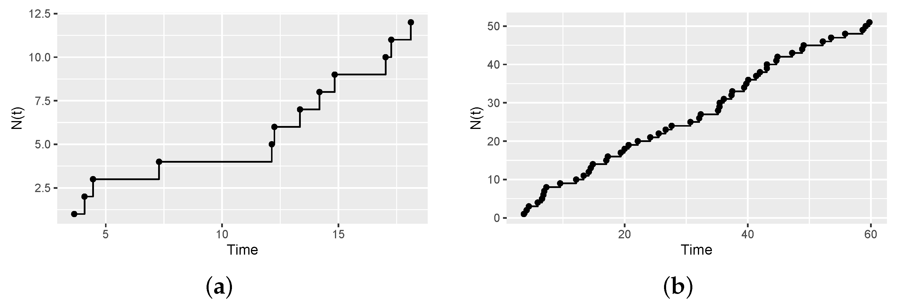
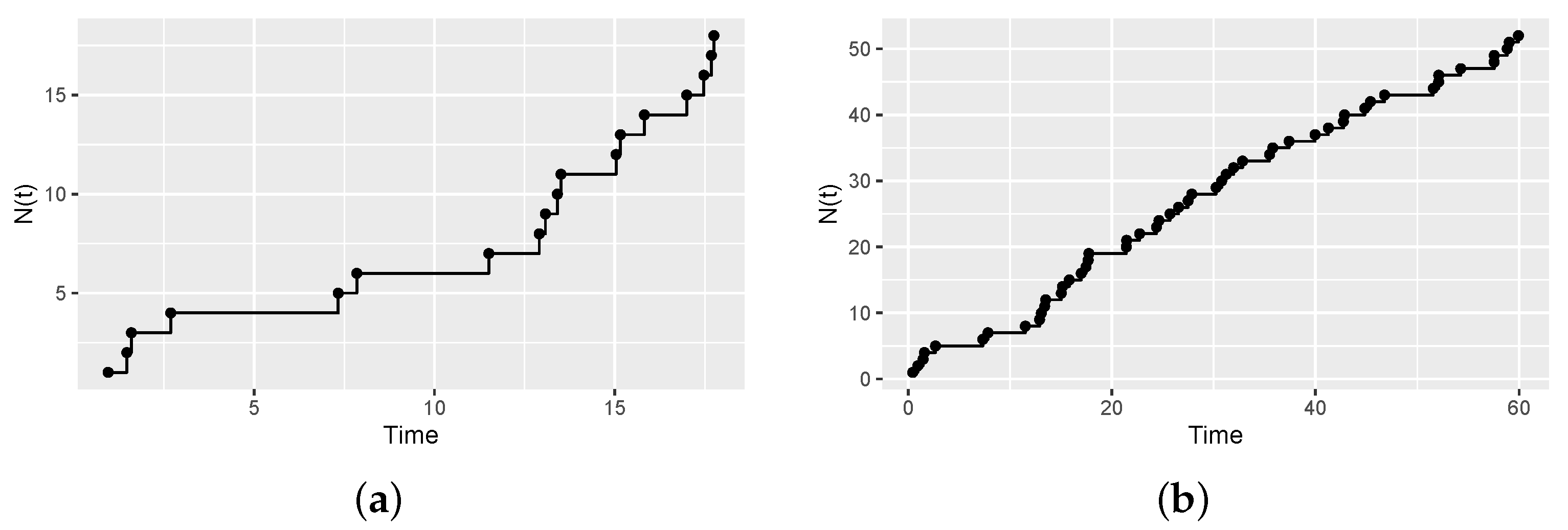
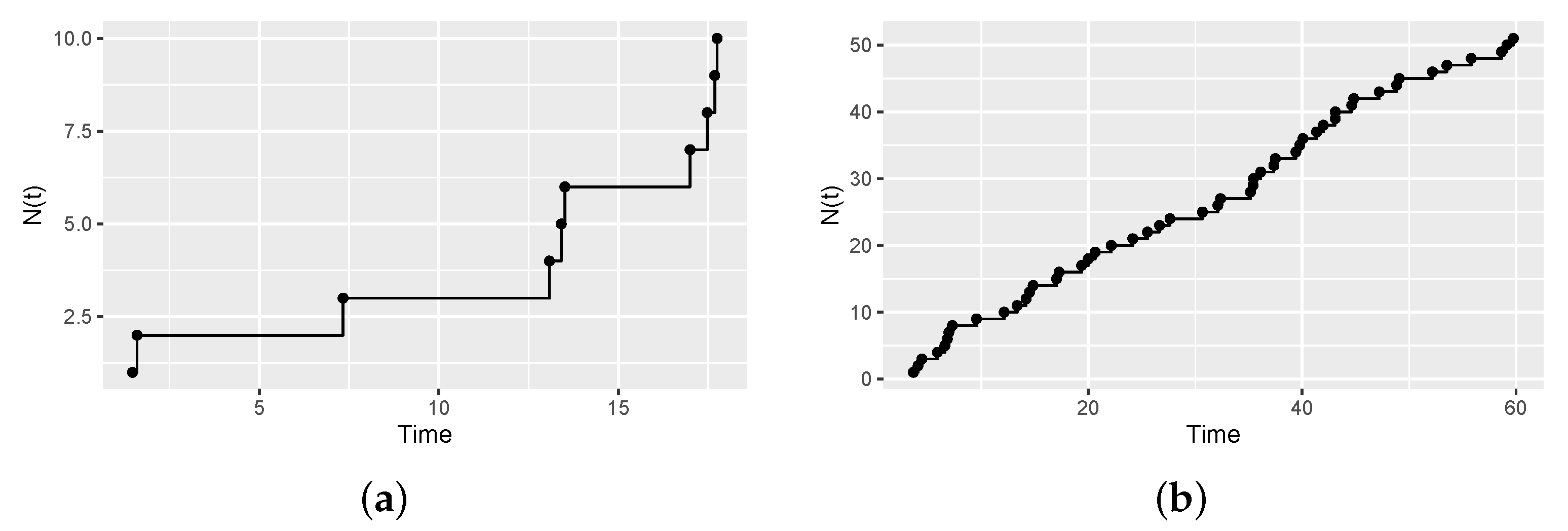
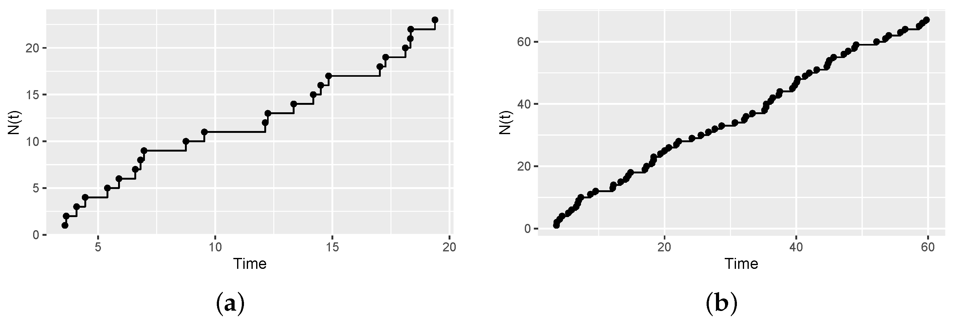
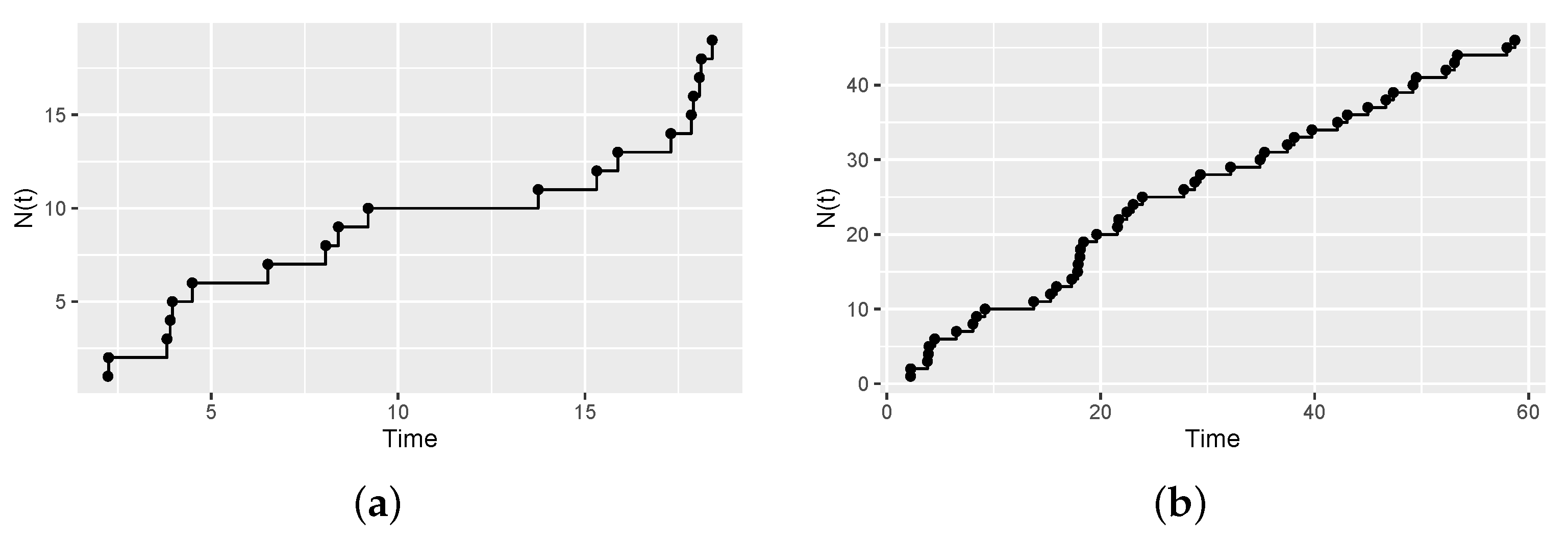
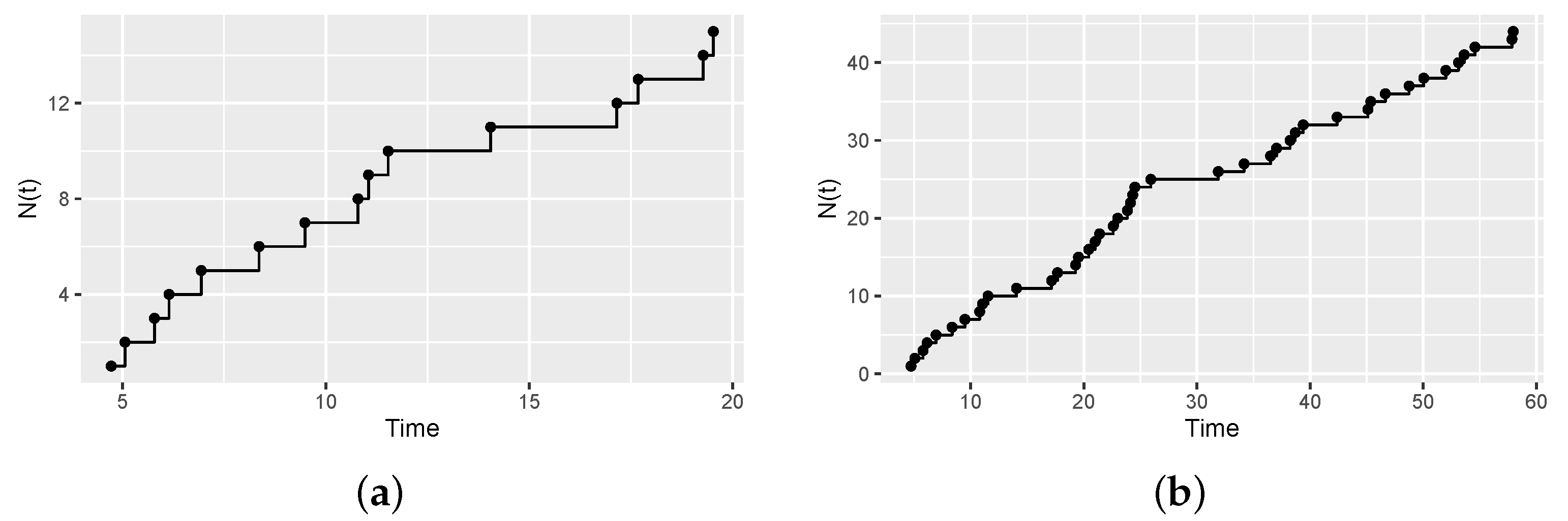
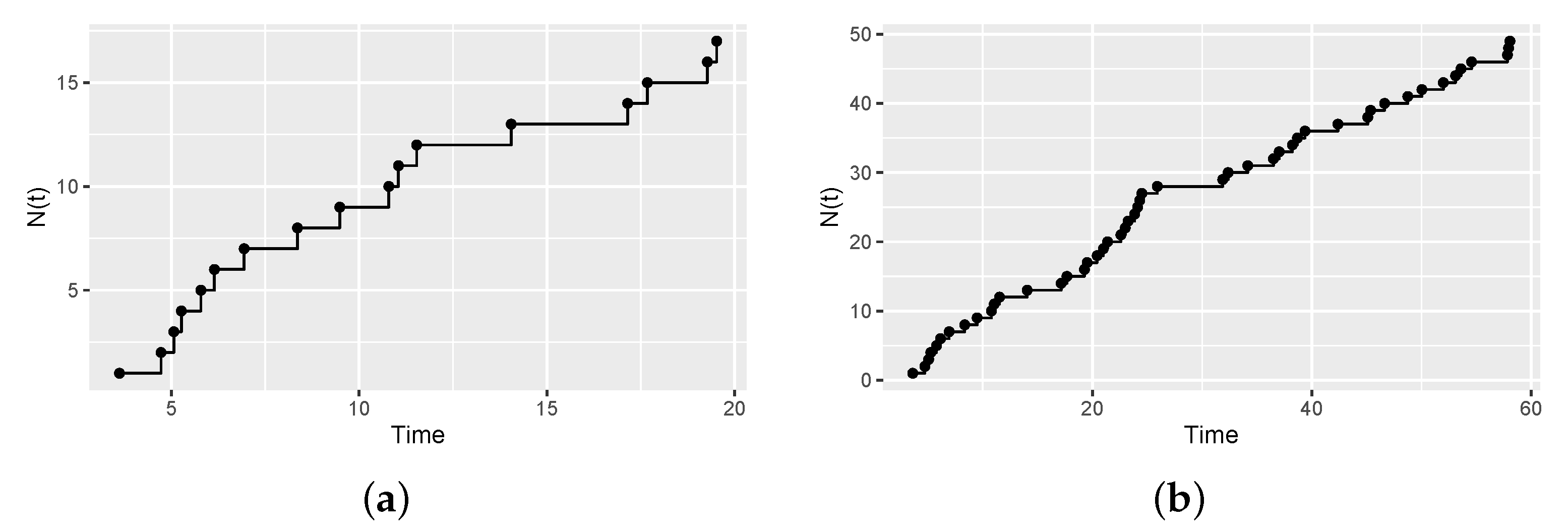
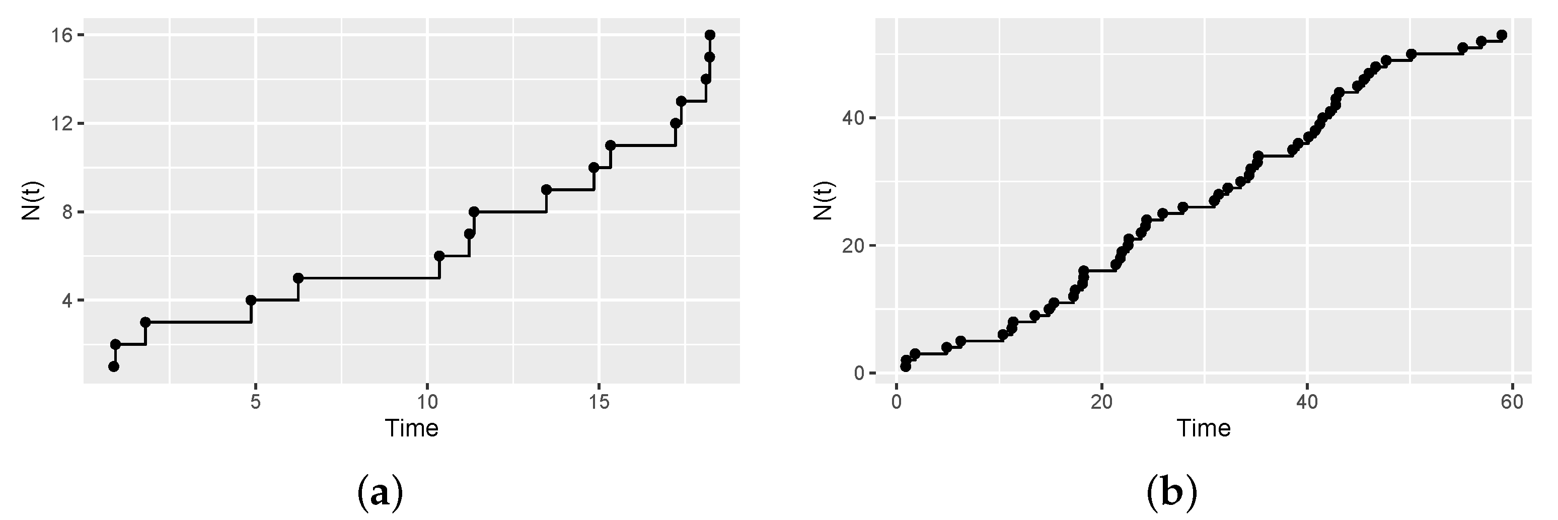
4. Simulation Studies

A more or less simple way to simulate a Cox Process is basically to simulate a non-homogeneous Poisson Process, using as intensity function one realization $\left\{\lambda \right(t):t\ge 0\}$ of the random field $\{\mathrm{\Lambda }(t):t\ge 0\}$, as suggested by Gabriel [39].

Following, for example, Ross [40], an algorithm that simulates an inhomogeneous Poisson process can be constructed, basically using the fact that this process can be generated by a random selection of times of a homogeneous Poisson Process of parameter $\lambda$. The idea, basically, is that if an event of the latter occurs at time t with probability ${\displaystyle \frac{\lambda \left(t\right)}{t}}$, then the process of counted events is an inhomogeneous Poisson process with a function of intensity $\left\{\lambda \right(t):t\ge 0\}$, where in particular, we restrict ourselves to a time horizon $[0,T]$.

The algorithm, in general terms, remains as:

Step 1

Start $t=0$ and $i=0$

Step 2

Generate $U_1,U_2\sim \mathrm{U}(0,1)$

Step 3

Make $t=t-{\displaystyle \frac{1}{\lambda }}·log\left(U1\right)$. If $t>T$, end up. Else, go to Step 4

Step 4

If $U_2\le {\displaystyle \frac{\lambda \left(t\right)}{t}}$, make $i=i+1$ y $S\left(i\right)=t$.

Step 5

Go to Step 2.

More details of it, as well as a more complete analysis and discussion, can be found in [40].

An adapted version of this algorithm has been used, by replacing the intensity function with the realization of the Folded Normal intensity, as suggested in [39], and implementing it in the free software R [38]. In particular, the Folded Normal intensity ($\lambda \left(t\right)t$) of the above algorithm has been simulated starting from the parameters of a Gaussian process.

Some trajectories provided by the simulated Cox process with Folded Normal intensity are represented in Figure 1, Figure 2, Figure 3, Figure 4, Figure 5, Figure 6, Figure 7 and Figure 8. In particular, Figure 1, Figure 2, Figure 3 and Figure 4 represent the trajectories provided by this process in the temporal intervals $[0,15]$ and $[0,20]$ by using the parameter $\mu =0$ and the exponential covariance function $k_Z\left(h\right)={\sigma }^2{e}^{-\beta \left|h\right|}$ with the combination of the parameters $(\sigma ;\beta )$ equal to $(1;1)$, $(9;1)$, $(1;0,15)$, and $(9;0,15)$, respectively. In all cases, we observe a common pattern given by periods with few events followed by periods with clusters of events. In other words, the events tend to cluster in time (two or more events occur in a close period of time), successively it follows a period with very few events and then a cluster of events occurs again. This pattern is evident when considering a short period of time such as $[0,T]=[0,20]$ as represented in Figure 1a, Figure 2a and Figure 3a, and for larger time horizons such as in Figure 1b, Figure 2b and Figure 3b where $[0,T]=[0,60]$ has been used. This makes us think that the proposed process could be adequate to model the phenomena which tend to form clusters in time such as earthquake events above a certain magnitude (for example the main earthquake and the strongest aftershocks), or some disease events. The parameters used in the simulation study have been chosen randomly by way of illustration. However, we have repeated the experiment with many other parameters and time horizons, and all of them showed the same common pattern. These results could be comparable with those processes considering clustering of events (see, for example, [41]).

Figure 5, Figure 6, Figure 7 and Figure 8 represent the trajectories of the simulated Cox process in the case that the intensity process is a family of independent variables following a Folded Normal law for different values of $\mu$ and ${\sigma }^2$. In particular, we considered the following combination of parameters $(\mu ;\sigma )$ for the periods $[0,20]$ and $[0,30]$: $(0;1)$, $(5;9)$, $(7;0.8)$ and $(15;169)$. As in the experiment with exponential covariance function, the independent case maintains the same pattern in short (with $[0,T]=[0,20]$) and longer (with $[0,T]=[0,60]$) temporal horizons.

As in the first set of simulations (where the exponential covariance was used), the same pattern representing periods with cluster of events followed by periods with few events is maintained for the case of independent variables.

5. Conclusions and Future Work

The Cox Processes provide a wide range of options for modeling specific processes over time. The particular case of the Cox Process with Folded Normal intensity, introduced in this work, presents the interesting characteristic of having analytically quite manageable results, and being able to adapt to different situations, depending on the values of its parameters. Based on the simulations, we observe that it adapts quite acceptably to specific processes that are characterized by having a concentration of occurrences in a certain period of time, and then prolonged intervals of “rest”, where “occurrences” are not observed. It is also appreciated that these events that occur in clusters have a slight tendency to repeat the same pattern at larger time horizons.

Regarding future work, we believe that there are many possibilities; some of these are to address this same process with different covariance functions, or to study the statistical inference about it, for example by estimators of moments, or Bayesian and classical estimators based on the maximum likelihood function. Moreover, the proposed process could be applied to real data for studying events that tend toward clustering in time such as earthquake or disease events. Another very interesting line of work may be to extend this process to space and time-space domains, and naturally from there to make classical and Bayesian inference. In this context, some methods have been proposed in he literature (see, for example, [42,43,44,45]). Additionally, some covariates could be included in the process following [46]. Lastly, more advanced algorithms for calculating the value of the Folded Normal intensity such that proposed by Chatterjee and Chakraborty [29] could be considered, in addition to studying new Cox processes with different intensity functions such as the Laplace Folded distribution proposed by Liu and Kozubowski [27].

References

1. Cox, D.R. Some statistical methods connected with series of events. J. R. Stat. Soc. Ser. B Stat. Methodol. 1955, 17, 129–157. [Google Scholar] [CrossRef]
2. Sheldon, M.R. Introduction to Prabability Models, 8th ed.; Academic Press: Cambridge, MA, USA, 2003. [Google Scholar]
3. Barry, R.J. Probabilidade: Um Curso em Naaível Intermediário; Instituto de Matemática Pura e Aplicada-CNPq, Projeto Euclides: Rio de Janeiro, Brasil, 1981. [Google Scholar]
4. Cox, D.R.; Miller, H.D. The Theory of Stochastic Processes; Imperial College: London, UK, 1967. [Google Scholar]
5. Parzen, E. Procesos Estocásticos; Holden Day Inc.: San Francisco, CA, USA, 1972. [Google Scholar]
6. Rozanov, Y.A. Procesos Aleatorios; Editorial Mir: Moscú, Russia, 1973. [Google Scholar]
7. Daley, D.J.; Vere-Jones, D. An Introduction to the Theory of Point Processes, Volume I: Elementary Theory and Methods, 2nd ed.; Springer: New York, NY, USA, 2003. [Google Scholar]
8. Møller, J.; Syversveen, A.R.; Waagepetersen, R.P. Log Gaussian Cox processes. Scand. J. Stat. 2008, 25, 451–482. [Google Scholar] [CrossRef]
9. Diggle, P.J.; Moraga, P.; Rowlingson, B.; Taylor, B.M. Spatial and Spatio-Temporal Log-Gaussian Cox Processes: Extending the Geostatistical Paradigm. Stat. Sci. 2013, 28, 542–563. [Google Scholar] [CrossRef]
10. Cuevas-Pacheco, F.; Møller, J. Log Gaussian Cox processes on the sphere. Spat. Stat. 2018, 26, 69–82. [Google Scholar] [CrossRef]
11. Aglietti, V.; Damoulas, T.; Bonilla, E. Efficient Inference in Multi-task Cox Process Models. arXiv 2018, arXiv:1805.09781. [Google Scholar]
12. Waagepetersen, R.; Guan, D.Y.; Jalilian, A.; Mateu, J. Analysis of multi-species point patterns by using multivariate log-Gaussian Cox processes. J. R. Statist. Soc. C 2016, 65, 77–96. [Google Scholar] [CrossRef]
13. Frías, M.P.; Torres-Signes, A.; Ruiz-Medina, M.D.; Mateu, J. Spatial Cox processes in an infinite-dimensional framework. TEST 2022, 31, 175–203. [Google Scholar] [CrossRef]
14. D’Angelo, N.; Siino, M.; D’Alessandro, A.; Adelfio, G. Local spatial log-Gaussian Cox processes for seismic data. AStA Adv. Stat. Anal. 2022. [Google Scholar] [CrossRef]
15. Benes, V.; Bodlak, K.; Møller, J.; Waagepetersen, R. Application of log-Gaussian Cox processes in disease mapping. In ISI International Conference on Environmental Statistics and Health; University of Santiago de Compostela: Santiago de Compostela, Spain, 2003. [Google Scholar]
16. Møller, J.; díaz-Avalos, C. Structured Spatio-Temporal Shot-Noise Cox Point Process Models, with a View to Modelling Forest Fires. Scand. J. Stat. 2010, 37, 2–25. [Google Scholar] [CrossRef]
17. Shirota, S.; Banerjee, S. Scalable Inference for Space-Time Gaussian Cox Processes. J. Time Ser. Anal. 2018, 40, 269–287. [Google Scholar] [CrossRef]
18. Walder, C.; Bishop, A. Gamma Gaussian Cox Processes. Methodology 2017. [Google Scholar] [CrossRef]
19. Flaxman, S.; Teh, Y.W.; Sejdinovic, D. Poisson intensity estimation with reproducing kernels. In Proceedings of the 20th International Conference on Artificial Intelligence and Statistics in Proceedings of Machine Learning Research, Fort Lauderdale, FL, USA, 20–22 April 2017; Volume 54, pp. 270–279. [Google Scholar]
20. Adams, R.P.; Murray, I.; MacKay, D.J.C. Tractable nonparametric Bayesian inference in Poisson processes with gaussian process intensities. In Proceedings of the 26th Annual International Conference on Machine Learning (ICML ’09), Montreal, QC, Canada, 14–18 June 2009; pp. 9–16. [Google Scholar]
21. Leone, F.C.; Nelson, L.S.; Nottingham, R.B. The folded normal distribution. Technometrics 1961, 3, 543–550. [Google Scholar] [CrossRef]
22. Tsagris, T.; Beneki, C.; Hassani, H. On the Folded Normal Distribution. Mathematics 2014, 2, 12–28. [Google Scholar] [CrossRef]
23. Psarakis, S.; Panaretos, J. On some bivariate extensions of the folded normal and the folded T distributions. J. Appl. Statist. Sci. 2001, 10, 119–136. [Google Scholar]
24. Chakraborty, A.K.; Chatterjee, M. On multivariate folded normal distribution. Sankhya Indian J. Stat. 2013, 75, 1–15. [Google Scholar] [CrossRef]
25. Kan, R.; Robotti, C. On Moments of Folded and Truncated Multivariate Normal Distributions. J. Comput. Graph. Stat. 2017, 26, 930–934. [Google Scholar] [CrossRef]
26. Nadarajah, S.; Bakar, A.; Anuar, S. New Folded Models for the Log-Transformed Norwegian Fire Claim Data. Commun. Stat.-Theory Methods 2015, 44, 4408–4440. [Google Scholar] [CrossRef]
27. Liu, Y.; Kozubowski, T.J. A folded Laplace distribution. J. Stat. Distrib. Appl. 2015, 2, 10. [Google Scholar] [CrossRef]
28. Subbotin, M.T. On the law of frequency of errors. Mat. Sb. 1923, 31, 296–301. [Google Scholar]
29. Chatterjee, M.; Chakraborty, A.K. A simple algorithm for calculating values for folded normal distribution. J. Stat. Comput. Simul. 2016, 86, 2. [Google Scholar] [CrossRef]
30. Liu, X.; Tian, G.L.; Fei, Y.; Shu, L.; Zhao, Q. Folded normal regression models with applications in biomedicine. J. Comput. Appl. Math. 2020, 379, 112941. [Google Scholar] [CrossRef]
31. Li, W.L.; Wei, A. Gaussian integrals involving absolute value functions. Inst. Math. Stat. Collect. 2009, 5, 43–59. [Google Scholar]
32. Møller, J.; Waagepetersen, R.P. Statistical Inference for Cox Processes. In Spatial Cluster Modelling; Chapman and Hall: New York, NY, USA, 2002; pp. 37–60. [Google Scholar]
33. Loéve, M. Probability Theory, 2nd ed.; Van Nostrand: Princeton, NJ, USA, 1960. [Google Scholar]
34. Tierney, L.; Kadane, J.B. Accurate Approximations for Posterior Moments and Marginal Densities. J. Am. Stat. Assoc. 1986, 81, 82–86. [Google Scholar] [CrossRef]
35. Az-Zo’bi, E. An approximate analytic solution for isentropic flow of an inviscid gas equations. Arch. Mech. 2014, 66, 203–212. [Google Scholar]
36. Az-Zo’bi, E. A reliable analytic study for higher-dimensional telegraph equation. J. Math. Comput. Sci. 2019, 18, 423–429. [Google Scholar] [CrossRef]
37. Az-Zo’bi, E.; Al-Amb, M.O.; Yildirim, A.; Alzoubi, W.A. Revised reduced differential transform method using Adomian’s polynomials with convergence analysis. Math. Eng. Sci. Aerosp. (MESA) 2020, 11, 827–840. [Google Scholar]
38. R Core Team. R: A Language and Environment for Statistical Computing; R Foundation for Statistical Computing: Vienna, Austria, 2021; Available online: https://www.R-project.org/ (accessed on 1 January 2020).
39. Gabriel, E. Représentation, Analyse et Simulation de Processus Ponctuels Spatio-Temporels; 1éres Rencontres R: Bordeaux, France, 2012. [Google Scholar]
40. Sheldon, M.R. Simulation, Second Edition: Programming Methods and Applications (Statistical Modeling and Decision Science); Academic Press: Cambridge, MA, USA, 1996. [Google Scholar]
41. Dassios, A.; Jang, J. The Distribution of the Interval between Events of a Cox Process with Shot Noise Intensity. J. Appl. Math. Stoch. Anal. 2008, 1–14. [Google Scholar] [CrossRef]
42. Shinichiro, S.; Gelfand, A.E. Inference for log Gaussian Cox processes using an approximate marginal posterior. arXiv 2016, arXiv:1611.10359. [Google Scholar]
43. Teng, M.; Nathoo, F.; Johnson, T. Bayesian Computation for Log-Gaussian Cox Processes—A Comparative Analysis of Methods. J. Stat. Comput. Simul. 2017, 87, 2227–2252. [Google Scholar] [CrossRef]
44. Goncalves, F.B.; Gamerman, D. Exact Bayesian inference in spatiotemporal Cox processes driven by multivariate Gaussian processes. J. R. Soc. Ser. B 2018, 80, 157–175. [Google Scholar] [CrossRef]
45. Walder, C.; Bishop, A.N. Fast Bayesian Intensity Estimation for the Permanental Process. In Proceedings of the 34th International Conference on Machine Learning (ICML’17), Sydney, Australia, 6–11 August 2017. [Google Scholar]
46. Kelling, C.; Murali, H. A two-stage Cox process model with spatial and nonspatial covariates. Spat. Stat. 2022, 51, 100685. [Google Scholar] [CrossRef]
Figure 1. Simulation of a Cox process with n Folded Normal intensity functio with parameters μ = 0 , σ 2 = 1 and with covariance function k Z ( h ) = e | h | for T = 20 (a) and T = 60 (b).
Axioms 11 00513 g001
Figure 2. Simulation of a Cox process with Folded Normal intensity with parameters μ = 0 , σ 2 = 9 and with covariance function k Z ( h ) = 9 e | h | for T = 20 (a) and T = 60 (b).
Axioms 11 00513 g002
Figure 3. Simulation of a Cox process with Folded Normal intensity function with parameters μ = 0 , σ 2 = 1 and with covariance function k Z ( h ) = e 0 , 15 | h | for T = 20 (a) and T = 60 (b).
Axioms 11 00513 g003
Figure 4. Simulation of a Cox process with Folded Normal intensity function with parameters μ = 0 , σ 2 = 9 and with covariance function k Z ( h ) = 9 e 0 , 15 | h | for T = 20 (a) and T = 60 (b).
Axioms 11 00513 g004
Figure 5. Simulation of a Cox process with Folded Normal intensity function with parameters μ = 0 , σ 2 = 1 and with covariance function k Z ( h ) = I { 0 } ( h ) for T = 20 (a) and T = 60 (b).
Axioms 11 00513 g005
Figure 6. Simulation of a Cox process with Folded Normal intensity function of parameters μ = 5 , σ 2 = 8 and with covariance function k Z ( h ) = 9 · I { 0 } ( h ) for T = 20 (a) and T = 60 (b).
Axioms 11 00513 g006
Figure 7. Simulation of a Cox process with Folded Normal intensity function of parameters μ = 7 , σ 2 = 0.8 and with covariance function k Z ( h ) = 0.8 · I { 0 } ( h ) for T = 20 (a) and T = 60 (b).
Axioms 11 00513 g007
Figure 8. Simulation of a Cox process with Folded Normal intensity function of parameters μ = 15 , σ 2 = 169 and with covariance function k Z ( h ) = 169 · I { 0 } ( h ) for T = 20 (a) and T = 60 (b).
Axioms 11 00513 g008
Publisher’s Note: MDPI stays neutral with regard to jurisdictional claims in published maps and institutional affiliations.