Spatiotemporal Analysis of the Background Seismicity Identified by Different Declustering Methods in Northern Algeria and Its Vicinity

Abstract

The main purpose of this paper was to, for the first time, analyse the spatiotemporal features of the background seismicity of Northern Algeria and its vicinity, as identified by different declustering methods (specifically: the Gardner and Knopoff, Gruenthal, Uhrhammer, Reasenberg, Nearest Neighbour, and Stochastic Declustering methods). Each declustering method identifies a different declustered catalogue, namely a different subset of the earthquake catalogue that represents the background seismicity, which is usually expected to be a realisation of a homogeneous Poisson process over time, though not necessarily in space. In this study, a statistical analysis was performed to assess whether the background seismicity identified by each declustering method has the spatiotemporal properties typical of such a Poisson process. The main statistical tools of the analysis were the coefficient of variation, the Allan factor, the Markov-modulated Poisson process (also named switched Poisson process with multiple states), the Morisita index, and the L–function. The results obtained for Northern Algeria showed that, in all cases, temporal correlation and spatial clustering were reduced, but not totally eliminated in the declustered catalogues, especially at long time scales. We found that the Stochastic Declustering and Gruenthal methods were the most successful methods in reducing time correlation. For each declustered catalogue, the switched Poisson process with multiple states outperformed the uniform Poisson model, and it was selected as the best model to describe the background seismicity in time. Moreover, for all declustered catalogues, the spatially inhomogeneous Poisson process did not fit properly the spatial distribution of earthquake epicentres. Hence, the assumption of stationary and homogeneous Poisson process, widely used in seismic hazard assessment, was not met by the investigated catalogue, independently from the adopted declustering method. Accounting for the spatiotemporal features of the background seismicity identified in this study is, therefore, a key element towards effective seismic hazard assessment and earthquake forecasting in Algeria and the surrounding area.

1. Introduction

The analysis of the strong spatiotemporal clustering of earthquakes is one of the most treated subjects in statistical seismology (e.g., [1,2,3,4,5,6,7,8,9,10,11,12,13,14,15,16,17] and several other references). Specifically, the temporal clustering is described as a significant increase in the earthquake intensity rate mainly caused by occurrences of large quakes and their aftershocks, whereas the spatial clustering is observed as earthquakes aggregate along the fault networks [8]. In general, earthquakes can be attributed to background and clustered seismicity components. The background class is constituted by independent, spontaneous, triggering, or mainshock events, whereas the clustered class is formed by foreshocks, aftershocks, swarms, triggered, or dependent events [18].

The most confronted issue so far in statistical seismology is the adequate identification of the background seismicity component, which is a crucial benchmark in seismic hazard and most seismicity studies (e.g., [19]). In this case, seismicity declustering, which is the discrimination process allowing the separation of earthquakes into background and clustered events, can be used to identify background earthquakes. However, different declustering methods are based on different physical and statistical hypotheses that may lead to diverse classification schemes for earthquakes (e.g., [19,20]). Since the background and the clustered seismicity components are highly superposed in time and space, the discrimination process is a very complicated task, especially when subjective definitions for aftershocks, foreshocks, and mainshocks are stated (e.g., [20,21,22]). Since the early works on catalogues declustering, mostly based on windowing methods (e.g., [23,24]), the resulting background seismicity is commonly expected to follow a temporally homogeneous and spatially inhomogeneous Poisson process; however, this feature depends on the declustering method hypotheses, the earthquake catalogue, the magnitude range, and the used statistical test [23,25]. Recently, some studies proved that the Poisson process with multiple states is a well suited model, which can better describe background seismicity in time, because of the many hidden overlapping processes in the rupture zone that may produce multilevel regimes (e.g., [11,22,26,27]). For instance, [11] found typical temporal variations in the background seismicity of Northeast Italy identified by Stochastic [5] and Nearest Neighbour declustering methods [28], which are in contradiction with the stationary Poisson assumptions. Specifically, three distinct average trends could be identified and were modelled by a switched Poisson process with three states. In [29], the possibility of the characterisation of the changes in the background seismicity trend was also discussed using the Markovian arrival process without any prior consideration of declustering.

In this paper, the Northern Algeria earthquakes catalogue is declustered to identify the background seismicity, by applying a variety of traditional windowing-based methods, including Gardner and Knopoff (GK) [23], Gruenthal (GRU) (e.g., [18]), and Uhrhammer (UHR) [24] methods, cluster-based methods such as the Reasenberg (REAS) [30] method, distance-based methods such as Nearest Neighbour (NN) method [9,28], and probability-based methods such as Stochastic Declustering (SD) method [5,6,31]. According to [32], the choice of declustering algorithm has considerable influence on the resulting background earthquakes catalogue, that is why we used various options in this article. Moreover, we suggest a procedure, based on different statistical tools, to compare the effectiveness of the adopted declustering methods, which were developed according to different statistical and physical assumptions. Specifically, we consider a set of statistical measures to quantify the presence of residual spatiotemporal clustering in each declustered catalogue, so that the most effective declustering method is the one associated with less residual clustering features. To this end, the Coefficient of Variation (CV), Allan Factor (AF) [33], Markov-Modulated Poisson Process (MMPP) (e.g., [11]), Morisita Index (MI) [34], and inhomogeneous version of L–function (e.g., [19]) were used, for the first time, to analyse the spatiotemporal patterns of the Algerian declustered catalogues, and to assess if the statistical properties of the space–time clustering are still present. Specifically, CV was used to assess the clustering behaviour, but without providing any information about the timescale ranges where the process can be reliably characterised as a clustered process [35]. The AF was used for assessing and measuring the time correlation in background seismicity. The AF has been already applied to the declustered earthquake catalogues of southern California and Switzerland [21], extracted using the classical declustering methods. As well as to seismicity, the AF measure was also applied to the analysis of time clustering of wave storms in the Mediterranean Sea [36] and the analysis of fire sequences recorded from 1969 to 2008 in Switzerland [37]. The MMPP was aimed at the study of the temporal changes in the background seismicity rate. This doubly stochastic model combined the Poisson process, which controls background event occurrences, with the Markov process, which is intended to describe the main changes linked to different stages in seismic activity (e.g., [11,38,39]). On the other hand, MI and L–function were used for assessing and measuring the spatial clustering of the resulting background seismicity. These spatial tools were applied to the space clustering analysis of Turkish earthquakes [19], which confirmed that the inhomogeneous Poisson process is the well–suited model to describe the Turkish declustered catalogues using SD and GK methods.

In this study, we propose and exemplify the collective use of this suite of measures as a tool for assessing the residual clustering in the background seismicity of Northern Algeria and its vicinity. The application of different declustering methods and different measures to the newly compiled catalogue of Northern Algeria provides several possible seismicity scenarios, namely a set of declustered catalogues (along with the corresponding clustering assessment), for the study of seismic hazard parameters in the study area.

The article is organised as follows. Section 2 describes the applied declustering methods to identify the background seismicity in the study region. Section 3 presents the mathematical formulations of the tools used to analyse background seismicity (CV, AF, MMPP, MI, and L–function). Section 4 describes the earthquake catalogue of Northern Algeria and its vicinity from 1950 to 2021, the main obtained results, and the discussion. Finally, Section 5 provides the conclusion.

2. Seismicity Declustering Methods

In this section, the used declustering methods, which are the most popular available in the literature, are presented. Specifically, we considered six different methods including three window-based methods, respectively due to GK, GRU, and UHR, the cluster-based method by REAS, the distance-based method named NN, and the probabilistic method named SD.

These declustering methods are based on different physical and statistical assumptions, which lead to non-unique identification of the background seismicity. This raised a number of questions, as discussed in [18,23]: Are the declustering methods effective in identifying random (Poissonian) sequences of independent events? In case non-Poissonian features are identified, is it due to the failure of declustering methods in removing all clustered events, or is the background seismicity inherently a non-Poissonian process? These questions are still open and unanswered. However, the identification of background seismicity is a primary step in many methodologies for seismic hazard assessment and earthquake forecasting, and a better understanding of declustering methods can significantly contribute developing more reliable approaches to these challenging goals.

2.1. Window-Based Methods

The window-based methods draw a space–time window around an earthquake of magnitude m, with space–time distances defined as a function of m. If a smaller earthquake is followed by a larger one in the same window, the window is reset to the larger magnitude. Then, the largest earthquake in the space–time window is considered to be a mainshock and is kept in the declustered catalogue, while the remaining events are removed. The window-based methods are the most straightforward and computationally fast techniques that can be used to separate clusters from background seismicity. The main disadvantage is that the window sizes are subjectively defined and often set to standard values [11]. In addition, these methods create significant gaps in the declustered catalogues, as shown in [40], and do not distinguish between direct and indirect aftershocks. The adopted space–time window sizes of GK, GRU, and UHR methods are given in

Table 1. Space–time window sizes of GK, GRU, and UHR methods.

Method	Space Window Size [Km]	Time Window Size [Day]
GK	${10}^{0.1238\ast m+0.983}$	$\left\{\begin{array}{c}{10}^{0.032\ast m+2.7389}, \mathrm{if} m\ge 6.5\\ {10}^{0.5409\ast m-0.547}, \mathrm{otherwise}\end{array}\right.$
GRU	$e^{1.77+{\left(0.037+1.02\ast m\right)}^2}$	$\left\{\begin{array}{cc}\left|e^{-3.95+{\left(0.62+17.32\ast m\right)}^2}\right|,& \mathrm{if} m\ge 6.5\\ {10}^{0.024\ast m+2.8}, & \mathrm{otherwise}\end{array}\right.$
UHR	$e^{-1.024+0.804\ast m}$	$e^{-2.87+1.235\ast m}$

[18], as implemented in the source codes are available in the ZMAP software [41,42].

2.2. Cluster-Based Method

The REAS method [30] distinguishes the aftershocks by joining earthquakes to clusters according to temporal and spatial interaction zones, using the Omori law [43] and the stress distribution, respectively (see [18] for further details). All linked events form a cluster, of which the largest earthquake is the mainshock and the remaining earthquakes are divided into foreshocks and aftershocks. To run the REAS algorithm, we used the standard input parameters (as specified in Table 3 of [18]), which correspond to the default parameters in the ZMAP software [41,42]. The lack of calibration of the parameters to the specific dataset might be a disadvantage of this method.

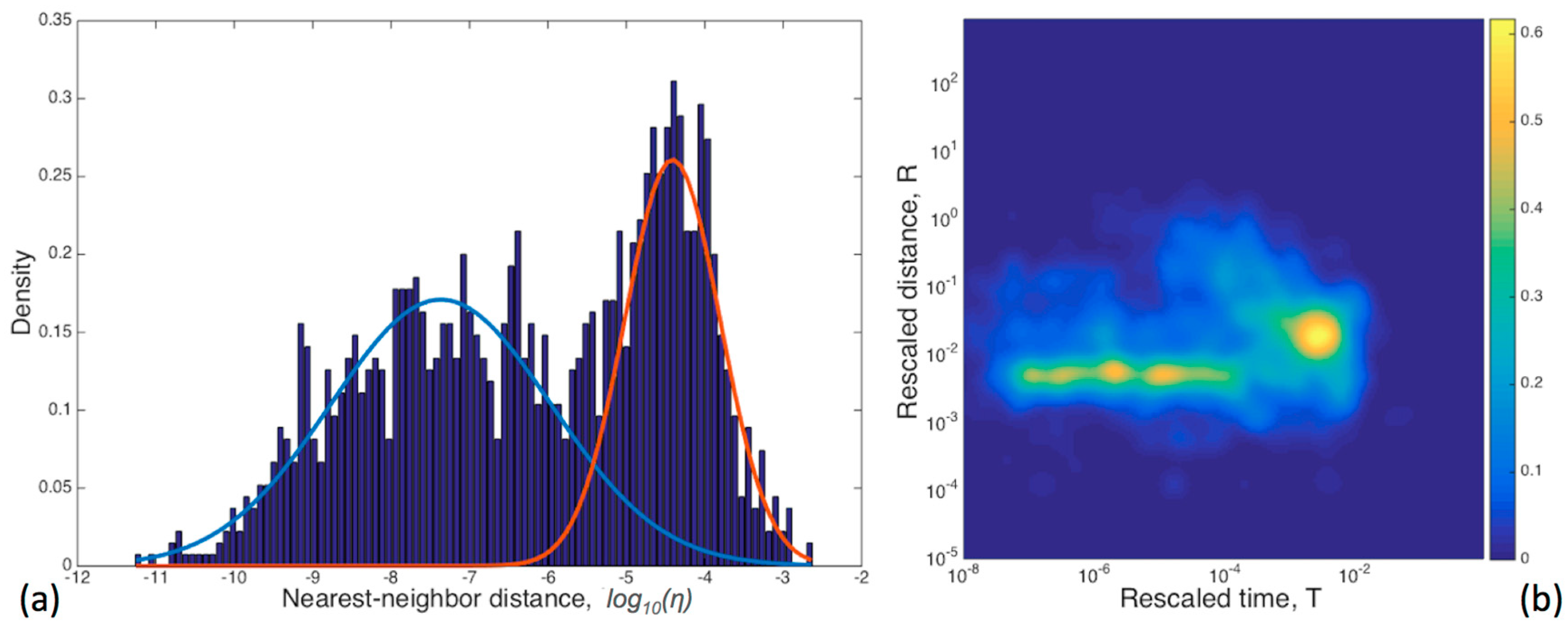
2.3. Nearest Neighbour Declustering Method

This method is based on the NN distance between pairs of earthquakes in a specific space–time–magnitude domain [10,28,40,44,45]. It is based on the asymmetric distance ${\eta }_{ij}$ between earthquakes $i$ and $j$ defined as:

$${\eta }_{ij}=\left\{\begin{array}{cc}{t}_{ij}{\left(r_{ij}\right)}^{d_f}{10}^{-b{m}_i},& t_{ij}>0\\ \infty & t_{ij}\le 0\end{array}\right.$$

(1)

where $t_{ij}=t_j-t_i$ is the interevent time, $r_{ij}$ is the spatial distance between epicentres, $d_f$ is the fractal dimension of epicentres, $b$ is the $b$–value of the Gutenberg–Richter (G–R) law [46], and $m_i$ is the magnitude of the $i$th earthquake. The unknown parameters $b$ and $d_f$ can be estimated by different methods (e.g., [47]). By following [44], the distance ${\eta }_{ij}$ can be decomposed into its time and space rescaled distances, respectively, defined as follows:

$$T_{ij}=t_{ij}{10}^{-qb{m}_i}\hspace{1em}\hspace{1em}{R}_{ij}={(r_{ij})}^{d_f}{10}^{-pb{m}_i}$$

(2)

where $\log {\eta }_{ij}=\log T_{ij}+\log R_{ij}$ and $q+p=1$.

Each event $j$ is associated with its unique parent $i$ by the following NN proximity [10]:

$$i=\underset{k:k<j}{argmin}{\eta }_{kj}$$

(3)

According to [8], the empirical distribution of the distance ${\eta }_{ij}$ shows a bimodal distribution that can be approximated as a mixture of two Gaussian distributions, one related to the background seismicity component and the other one to the clustered seismicity component. A threshold distance ${\eta }_0$ is chosen as the intersection point of the two estimated Gaussian distributions. Each event $j$ and its parent $i$ are considered weakly linked if ${\eta }_{ij}>{\eta }_0$, and strongly linked otherwise. The removal of weak links leads to the identification of earthquake clusters, where the largest magnitude event is considered as the mainshock, and the rest of the events constitute the foreshocks and aftershocks. The main advantage of the NN method is its soft parameterization, which requires fitting to the data a low number of parameters. Moreover, differently from the window-based methods, NN provides information about the internal structure of the clusters, namely all the subordinate levels of aftershocks.

2.4. Stochastic Declustering Method

The first ideas on the probabilistic discrimination between background and clustered seismicity components that mimic the whole earthquake activity were presented by [2]. Later, [5] developed an effective probabilistic version of the declustering method using the space–time Epidemic Type Aftershock Sequence (ETAS) model. Given an earthquake catalogue that collects the temporal occurrence $t_i$, longitude $x_i$, latitude $y_i$, and magnitude $m_i$ of all the earthquakes in a seismic region ($i=1,\dots ,n$), the standard expression of the conditional intensity function of the ETAS model as given by [4] is presented as a superposition of background $\mu \left(x,y\right)$ and clustered $\left\{\lambda \left(t,x,y\right)-\mu \left(x,y\right)\right\}$ intensity functions as follows:

$$\lambda \left(t,x,y\right)=\mu \left(x,y\right)+{{\displaystyle \sum }}_{\left\{i: t_i<t\right\}}\kappa \left(m_i\right)g\left(t-t_i\right)f\left(x-x_i,y-y_i|m_i\right)$$

(4)

where

$$\mu \left(x,y\right)=\nu u\left(x,y\right)$$

(5)

$$\kappa \left(m\right)=A{e}^{\alpha \left(m-m_c\right)}$$

(6)

$$g\left(t\right)=\left\{\begin{array}{cc}\left(p-1\right)c^{p-1}{\left(t+c\right)}^{-p}, & \mathrm{for} t>0\\ 0& \mathrm{otherwise}\end{array}\right.$$

(7)

$$f\left(x,y|m\right)=\frac{q-1}{\pi D{e}^{\gamma \left(m-m_c\right)}}{\left[1+\frac{x^2+y^2}{D{e}^{\gamma \left(m-m_c\right)}}\right]}^{-q},\hspace{1em}q>1, \gamma >0,\hspace{1em}D>0$$

(8)

where $m_c$ is the completeness magnitude, $\mu \left(x,y\right)$ is the spatial background intensity, $u\left(x,y\right)$ is an intensity function taking account of the spatial inhomogeneity in background seismicity, $\kappa \left(m\right)$ is the expected number of events triggered from an event of magnitude $m$, $g\left(t\right)$ and $f(x,y|m)$ are the probability density functions of occurrence times and location distribution of the triggered events, respectively. An iterative algorithm for Maximum Likelihood Estimation (MLE) simultaneously provides the model parameters $\theta =\left(\nu ,A,\alpha ,p,c,q,D,\gamma \right)$, the background rate $\mu \left(x,y\right)$, and the branching (triggering) structure of clusters (Algorithm 1 in [5]; further details are given in [6,31]). The latter is expressed in terms of the probability that the earthquake $j$ is triggered by a previous earthquake $i$, the probability that earthquake $j$ is a triggered earthquake, and the probability that earthquake $j$ is a background event, namely:

$${\rho }_{ij}=\frac{\kappa \left(m_i\right)g\left(t_j-t_i\right)f\left(x_j-x_i,y_j-y_i|m_i\right)}{\lambda \left(t_j, x_j,y_j\right)}$$

(9)

$${\rho }_j={{\displaystyle \sum }}_{\{i: t_i<t_j\}}{\rho }_{ij}$$

(10)

$${\phi }_j=1-{\rho }_j$$

(11)

By using the thinning procedure [5], it is possible to simulate many realizations of the background seismicity. Although SD does not identify a unique declustered catalogue, its advantage is that no information is lost in the declustering procedure; rather, a new item, the probability, is added to the parameters of the events in the catalogue to quantify the uncertainty [6]. However, this complicates the comparison of the results obtained from the SD method with those obtained from other methods. In our case study, a reasonable choice was to consider the realization obtained by the most probable background events according to the estimated probabilities based on Equations (9)–(11). Parenthetically, the background events in GK, GRU, UHR, REAS, and NN methods are defined as the mainshocks of the identified earthquake clusters. The SD method acts differently because it assigns the initiating (or independent) event of each cluster to the background seismicity, which is often not the mainshock.

3. Statistical Measures for Spatiotemporal Analysis of Background Earthquakes

Various statistical measures are described in this section, in order to investigate the space–time characteristics of occurrences of background earthquakes. We present five statistical tools: CV, AF, MMPP, MI, and the inhomogeneous version of L–function.

3.1. Coefficient of Variation

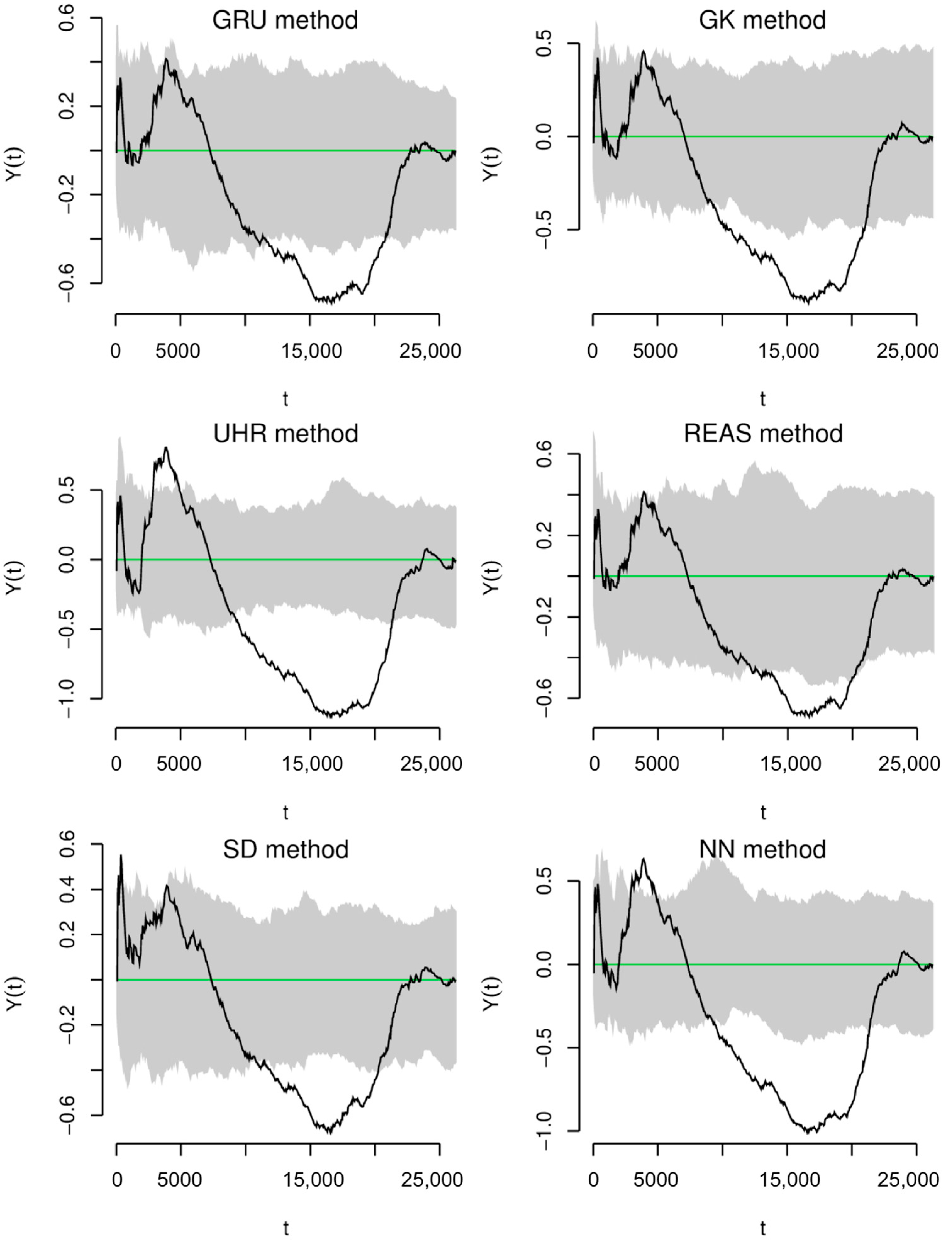
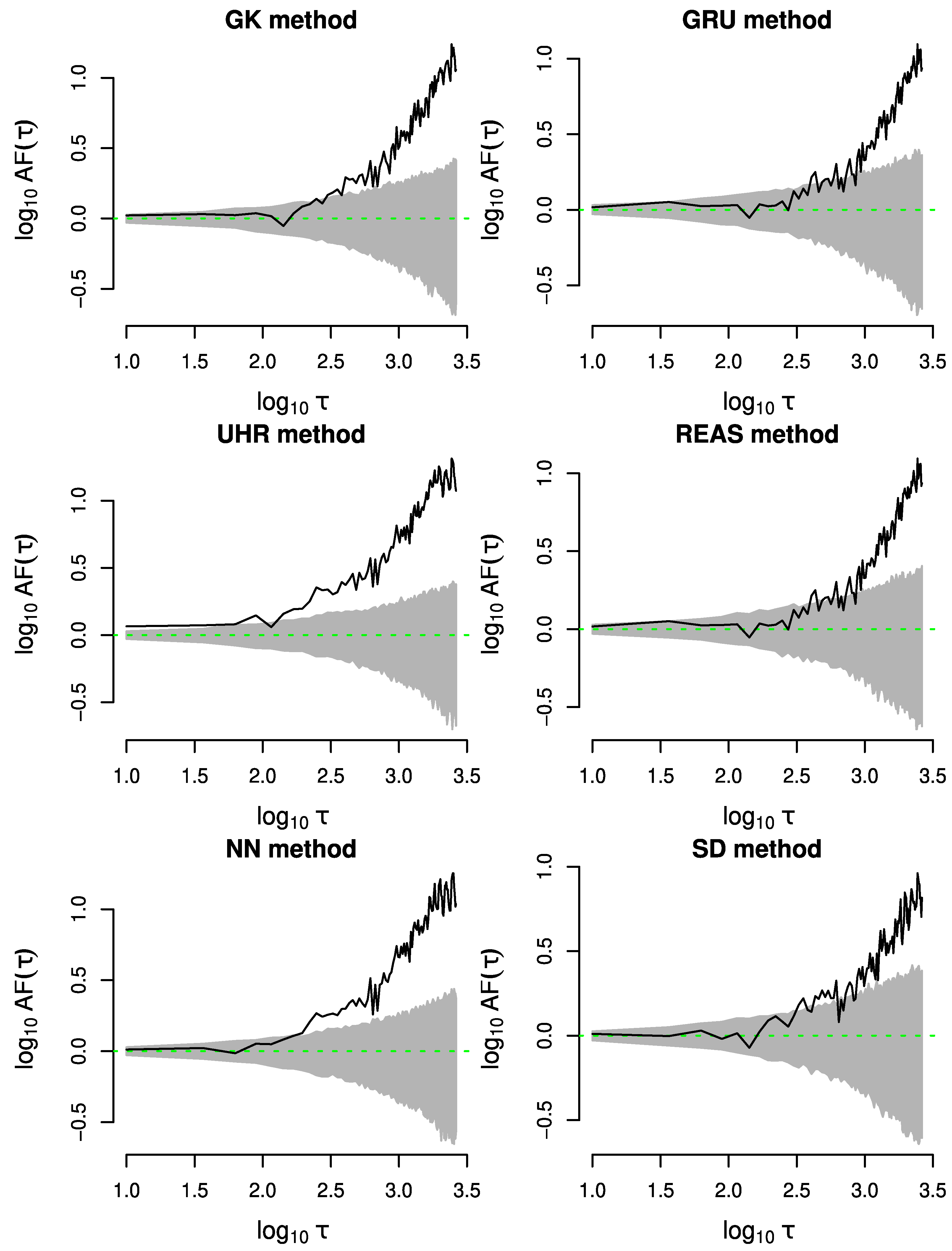
The CV, which is defined as the ratio between the standard deviation and the mean of the interevent times between consecutive earthquakes, is the most used measure to assess the clustering behaviour in earthquake sequences (e.g., [48]). It is given as follows:

$$CV=\frac{\sigma \left(\tau \right)}{Mean\left(\tau \right)}$$

(12)

where $\sigma \left(\tau \right)$ and $Mean\left(\tau \right)$ are the standard deviation and the mean of interevent time $\tau$, respectively. For a Poissonian process, $\sigma \left(\tau \right)=Mean\left(\tau \right)$ and hence, $CV=1$, and for a clustered process, $\sigma \left(\tau \right)>Mean\left(\tau \right)$ which leads to $CV>1$. However, this coefficient does not give any information about the time scale ranges where the process has clustered or Poissonian behaviours (e.g., [49]). In this case, the Poissonian behaviour can be further investigated using the following empirical measure (e.g., [19]):

$$Y\left(t\right)=\frac{N\left(t\right)}{\sqrt{\lambda t}}-\sqrt{\lambda t}$$

(13)

where $N\left(t\right)=\#\left\{t_i\text{:} t_i\le t\right\}$ is the number of events in a catalogue occurring up to time $t$ and $\lambda$ is the rate of a homogeneous Poisson process in time. Under the homogeneous Poissonian assumption, $Y\left(t\right)$ is of zero mean and unit variance [19]. Monte Carlo simulations are performed to obtain confidence bands of $Y\left(t\right)$ under this hypothesis and to compare them with the observed $Y\left(t\right)$.

3.2. Allan Factor

To investigate the clustering pattern in earthquake occurrence times, which are supposed to be a realization of a temporal point process [50], the AF measure can be used. By splitting the time axis into a number of windows of equal length $\tau$, and letting $N_k$ represent the number of events falling into the $k$th window, $\langle N_k\rangle$ forms a discrete random process of nonnegative integers [21,35,49,51]. In this case, the AF measure is defined as the variance of successive counts for a specified counting time $\tau$, divided by twice the mean number of events in the same counting time $\tau$, and is given as follows:

$$AF\left(\tau \right)=\frac{E\left[{(N_{k+1}\left(\tau \right)-N_k\left(\tau \right))}^2\right]}{2E[N_k\left(\tau \right)]}$$

(14)

where $E\left[.\right]$ indicates the expectation symbol. For a homogeneous Poisson process, $AF\left(\tau \right)$ is approximately equal to $1$ at all timescales; in this case, the corresponding plot of $AF\left(\tau \right)$ versus $\tau$ will appear approximately flat. Otherwise, the clustered behaviour is detected if $AF\left(\tau \right)>1$. In the special case of a fractal point process, $AF\left(\tau \right)$ increases with the timescale $\tau$ as a power law [21,35,49,52]:

$$AF\left(\tau \right)=1+{\left(\tau /{\tau }_1\right)}^{\alpha }$$

(15)

where $0<\alpha <3$ is the fractal exponent which quantifies the clustering intensity, and ${\tau }_1$ is the fractal onset time that marks the lower limit above which the fractal behaviour can be detected.

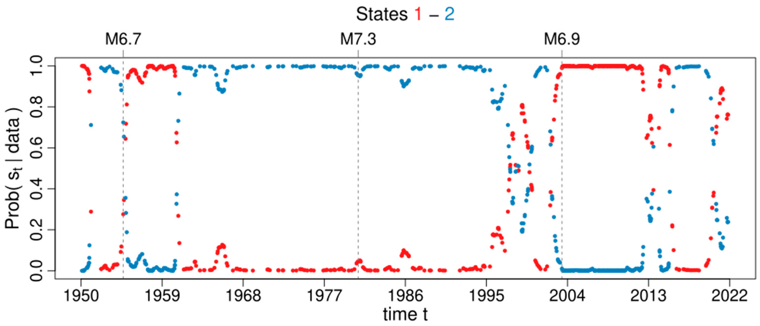
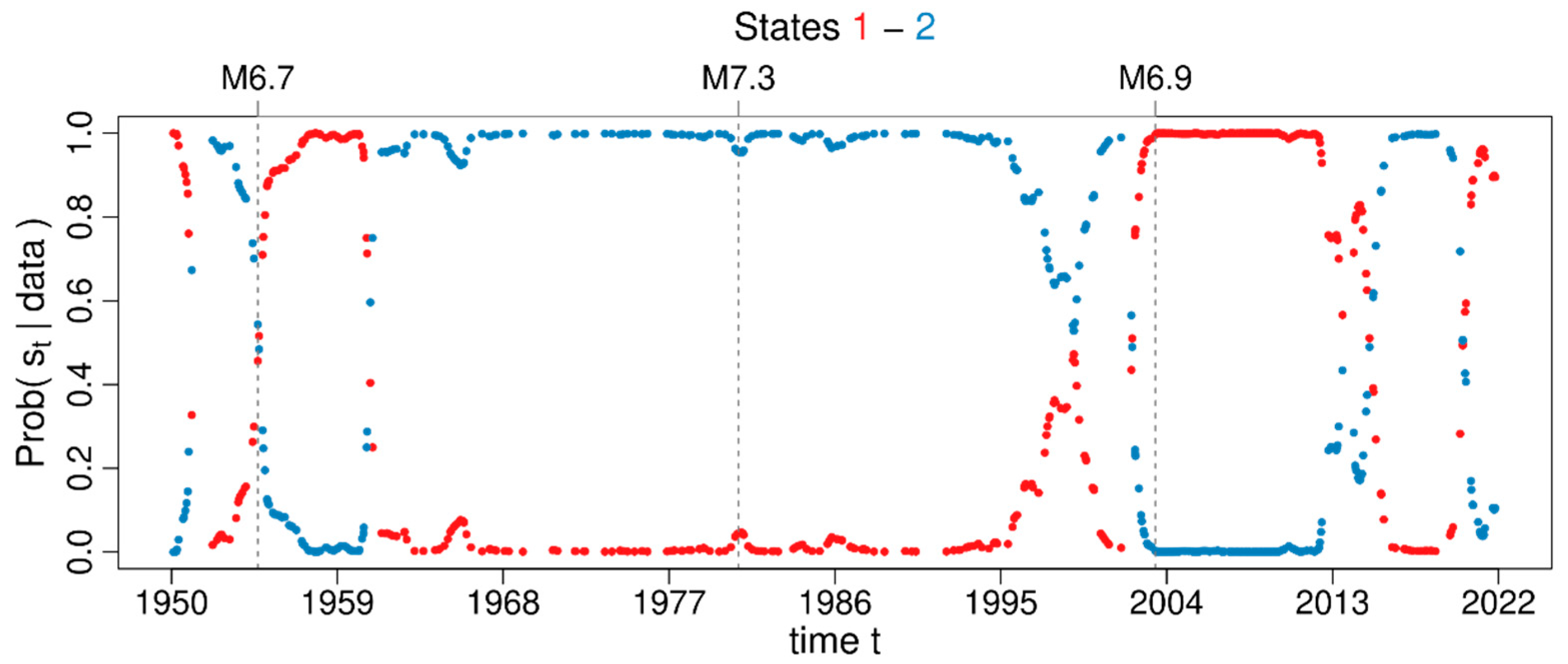
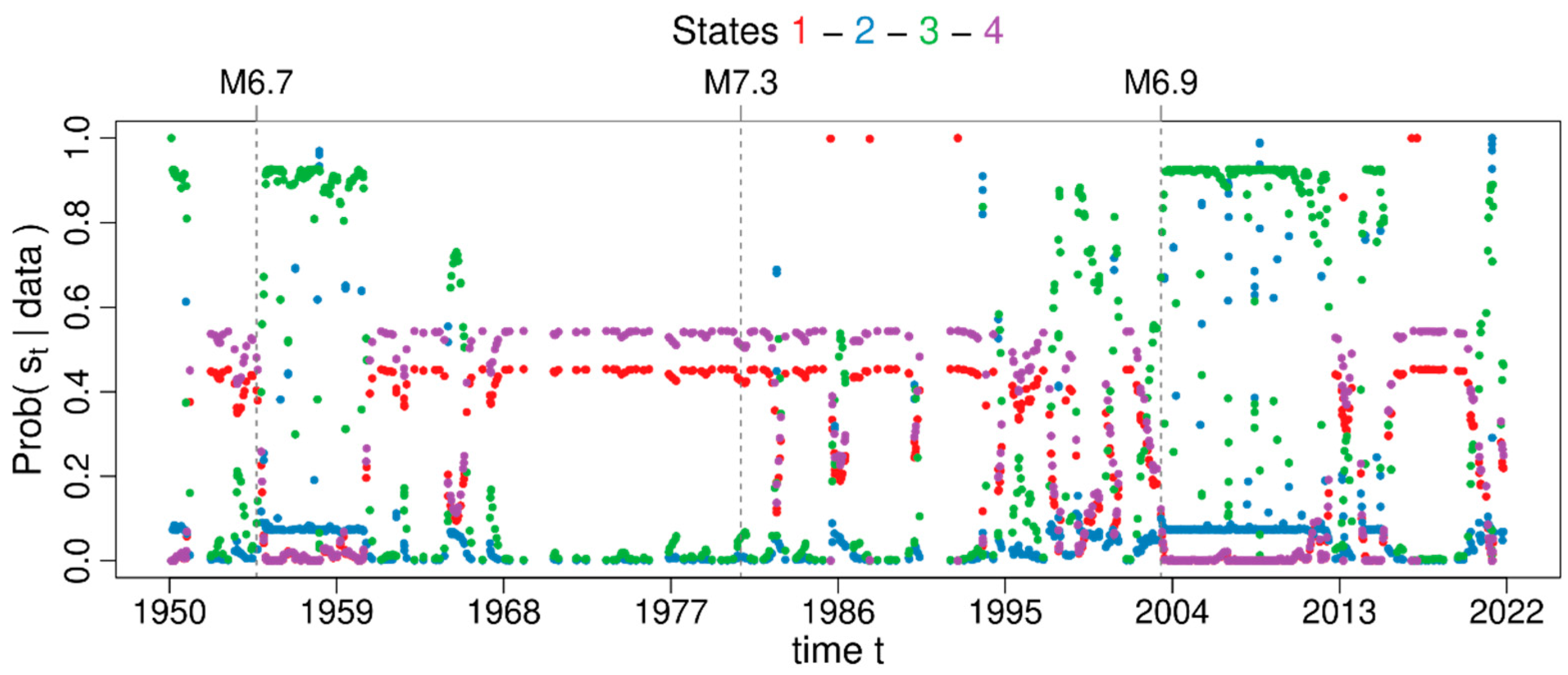
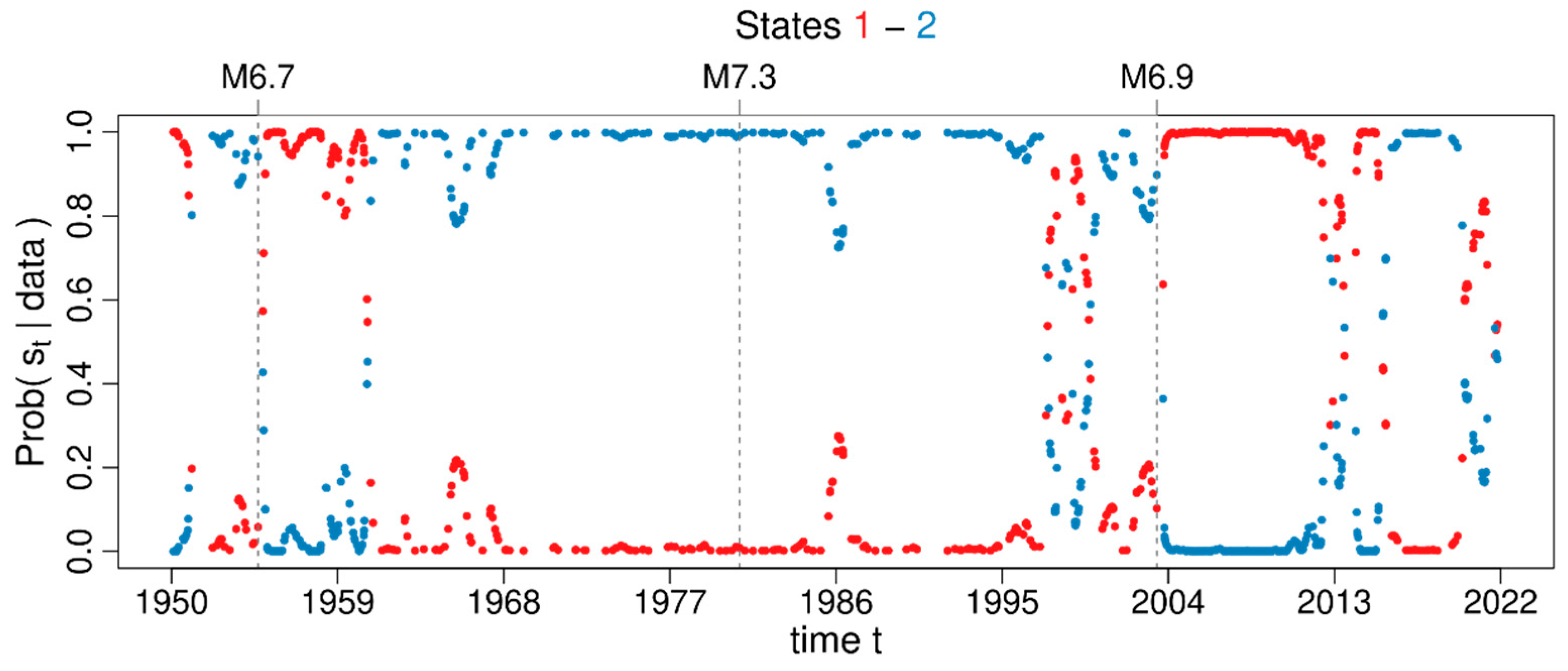
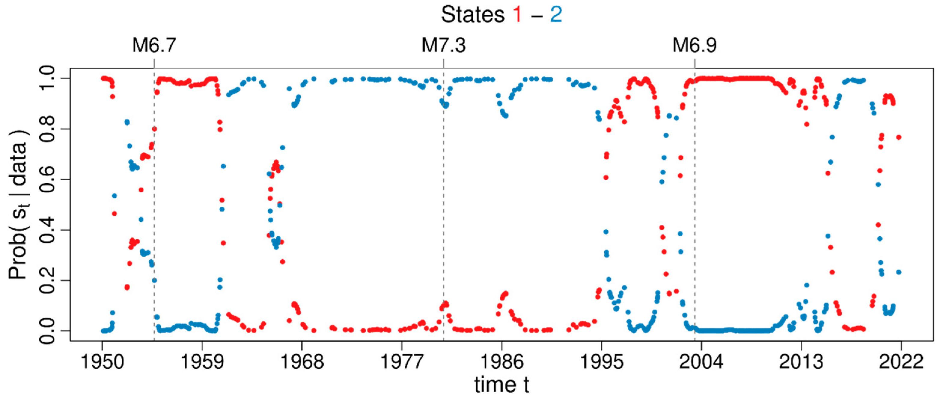
3.3. Markov Modulated Poisson Process

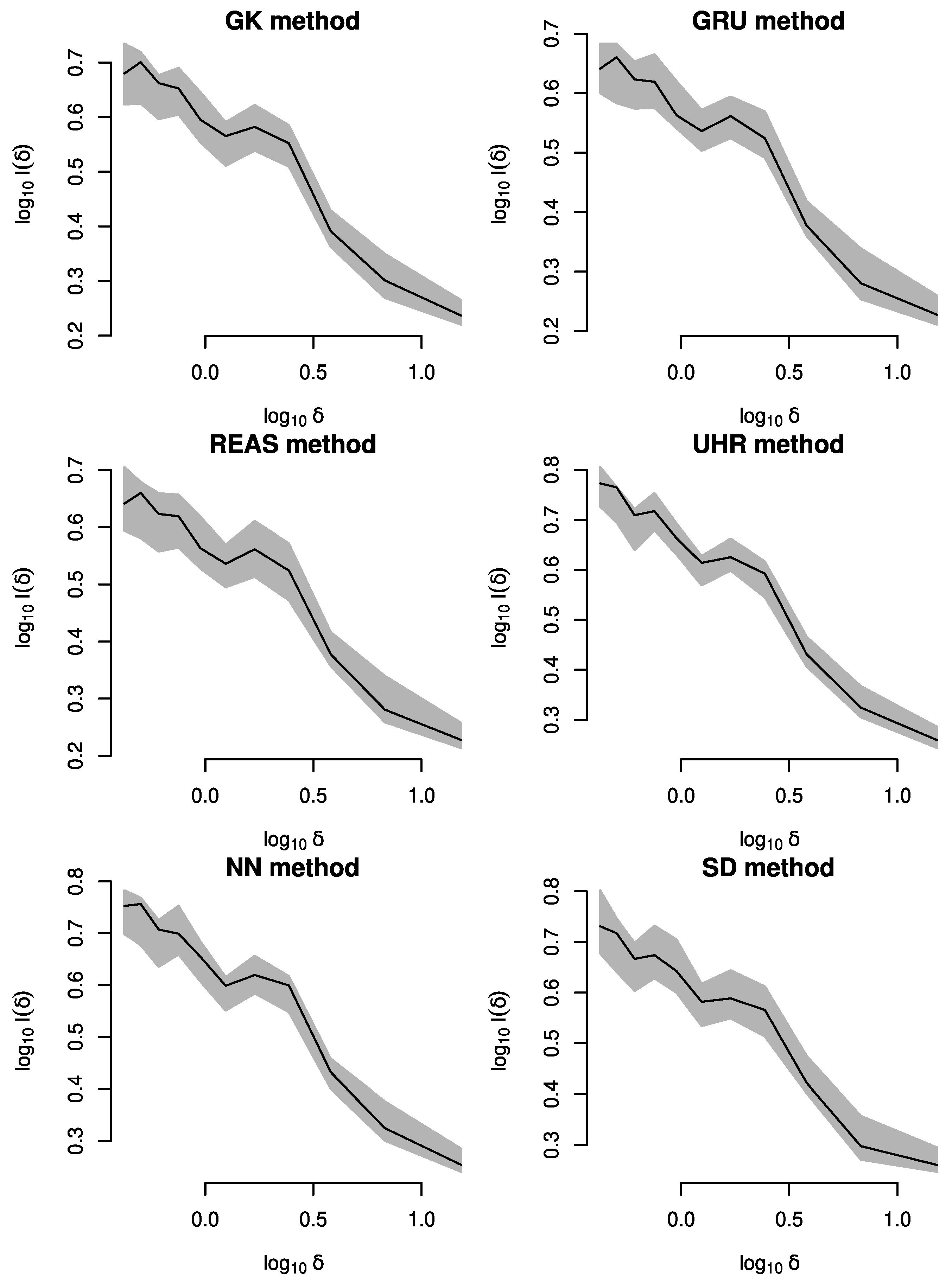
An MMPP is a suitable process for describing dynamic systems in which the observations follow a Poisson process, whose occurrence rate switches between a finite number of values simultaneously to change in the state of a Markov process [53,54]. Mathematically, the state process $X\left(t\right)$, $t>0$ is an irreducible homogeneous Markov process with a finite state space $S=\left\{1,2,\dots ,K\right\}$ such that

$$X\left(t\right)=s_j\hspace{1em}\hspace{1em}\forall t\in \left[{\tau }_j,{\tau }_{j+1}\right)$$

(16)

where $\left\{s_j\in S:j=0,1,2,\dots \right\}$ denotes the sequence of states visited by the state process at the transition times ${\tau }_0\le {\tau }_1\le {\tau }_2\le \dots .$ The observation process $N\left(t\right)$ is a nonhomogeneous Poisson process with intensity given by

$$\lambda \left(t\right)={\lambda }_{s_j}\hspace{1em}\hspace{1em}\forall t\in \left[{\tau }_j,{\tau }_{j+1}\right)$$

(17)

where ${\lambda }_1$, ${\lambda }_2$,…, ${\lambda }_K$ denote the earthquake occurrence rates associated with the Markovian states $1, 2,\dots , K$.

By assuming a $K$–MMPP model (MMPP with $K$ states), the intensities ${\lambda }_1$, ${\lambda }_2$,…, ${\lambda }_K$ of the Poisson process are estimated by the Baum–Welch algorithm using the R package HiddenMarkov [55]. Moreover, this package returns the probabilities $P(X\left(t\right)=s |t_1,t_2,\dots ,t_n)$, defined as the probabilities that the state process is in state $s$ at time $t$ given the earthquake occurrence times $t_1, t_2,\dots , t_n$. Since the number of hidden states $K$ is unknown, we selected the best–fitting model among different MMPP models, $K\ge 1$, using the Bayesian Information Criterion (BIC) [56].

3.4. Morisita Index

MI is used to investigate the presence of space clustering behaviour in earthquake patterns (e.g., [21,57,58]). Given a grid of $M$ cells of variable size $\delta$, MI is defined as follows:

$$I_{\delta }=M\frac{{{\displaystyle \sum }}_{i=1}^M{n}_i\left(n_i-1\right)}{N\left(N-1\right)}$$

(18)

where $n_i$ is the number of points falling in the $i$th cell and $N$ is the total number of earthquakes. To draw the plot relating each $I_{\delta }$ to its corresponding $\delta$, it is recommended to start with a relatively high cell size $\delta$ and the corresponding algorithm is iterated for decreasing $\delta$ until a minimum value is reached. According to [21], $I_{\delta }$ fluctuates around $1$ in the case of Poissonian behaviour and decreases to zero in the case of clustered behaviour. Additionally, the Morisita slope $S_2$ is considered. It is defined as the slope of the linear regression fitting ${\log }_{10}{I}_{\delta }$ and ${\log }_{10}\delta$ [21]:

$$\underset{\delta \to +\infty }{\mathit{lim}}\left|\frac{{\log }_{10}{I}_{\delta }}{{\log }_{10}\delta }\right|\approx S_2$$

(19)

This slope quantifies the degree of clustering: the greater $S_2$, the greater the clustering degree in the earthquake sequence.

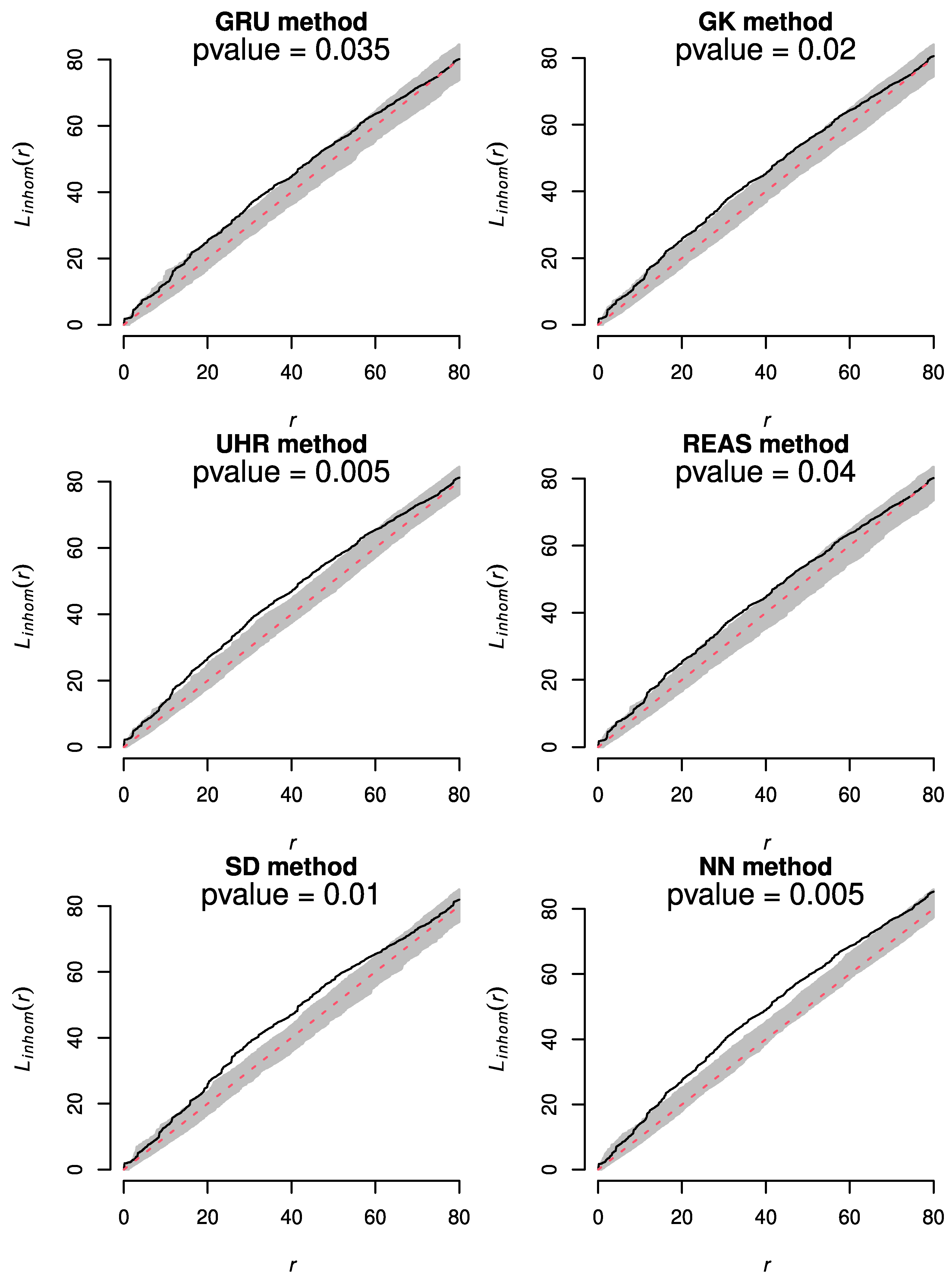
3.5. Inhomogeneous Version of L-Function

An inhomogeneous version of Besag’s L-function [59] can be used to examine whether the spatial point process of locations of earthquake epicentres follows a spatially inhomogeneous Poisson process with the seismicity rate $\lambda \left(x,y\right)$ [19]. The empirical L-function given as the transformation of the Ripley K-function [59] is defined as follows:

$$L\left(r\right)=\sqrt{\frac{K\left(r\right)}{\pi }}=\sqrt{\frac{1}{\pi }{{\displaystyle \sum }}_{i=1}^N{{\displaystyle \sum }}_{j\ne i=1}^N\frac{ {\rm I}\left\{{\left(x_i-x_j\right)}^2+{\left(y_i-y_j\right)}^2\le r^2\right\}}{\lambda \left(x_i,y_i\right)\lambda \left(x_j,y_j\right)\left|{\mathcal{M}}_i\cap {\mathcal{M}}_j\right|}}, r\ge 0$$

(20)

where ${\rm I}$ is the indicator function that takes 1 when the condition is true and 0 otherwise, $K\left(r\right)$ is the expected value of the sum of $1/\left(\lambda \left(x_i,y_i\right)\right)$ over all longitudes $x_i$ and latitudes $y_i$ that are within a distance $r$, ${\mathcal{M}}_i=\left\{\left(x-x_i,y-y_i\right):\left(x,y\right)\in \mathcal{M}\right\}$ is the translation of the studied geographical region $\mathcal{M}$ by $\left(x_i,y_i\right)$, and $\left|{\mathcal{M}}_i\cap {\mathcal{M}}_j\right|$ denotes the area of ${\mathcal{M}}_i\cap {\mathcal{M}}_j$. For an inhomogeneous Poisson process with intensity function $\lambda \left(x,y\right)$, $L\left(r\right)=r$ for all distances $r\ge 0$. Whereas the values $L\left(r\right)>r$ indicate the positive pairwise correlation (clustering/aggregation) at a distance $r$ and the values $L\left(r\right)<r$ indicate the negative pairwise correlation (repulsion) [19]. The following test statistic [19], $D=\underset{0<r<R}{\max }\frac{\left|L\left(r\right)-L_{poiss}\left(r\right)\right|}{r}$, can be used in the calculation of the $p$-values for the null hypothesis of spatially inhomogeneous Poisson assumption, using the theoretical Poisson $L_{poiss}\left(r\right)$ as a reference.

4. Statistical Analysis of the Declustered Catalogues

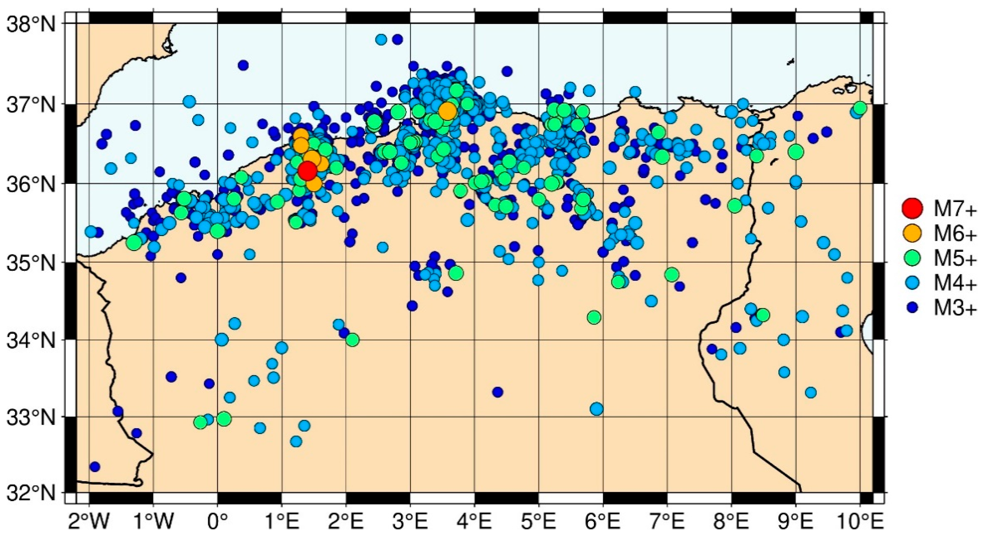
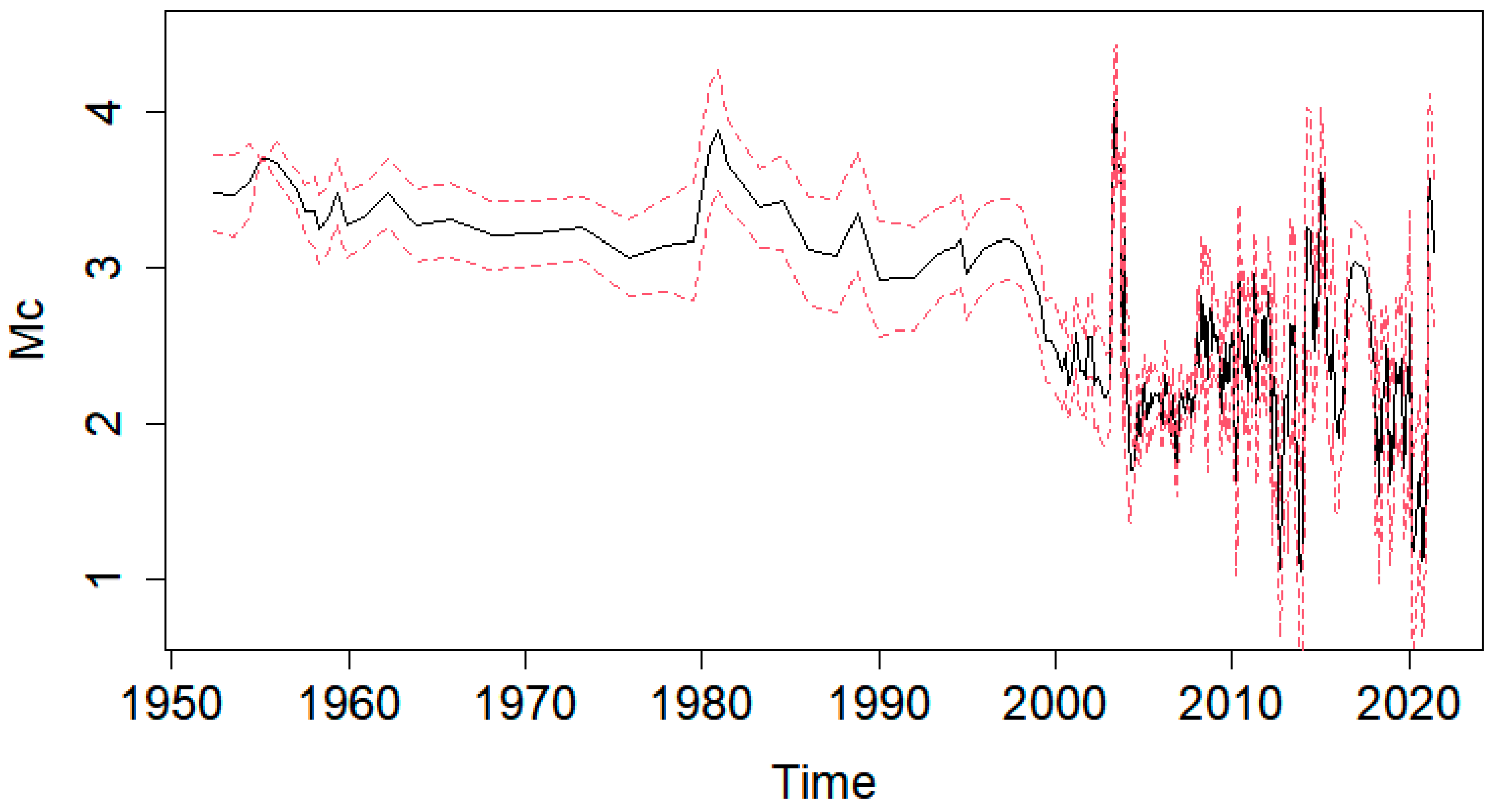
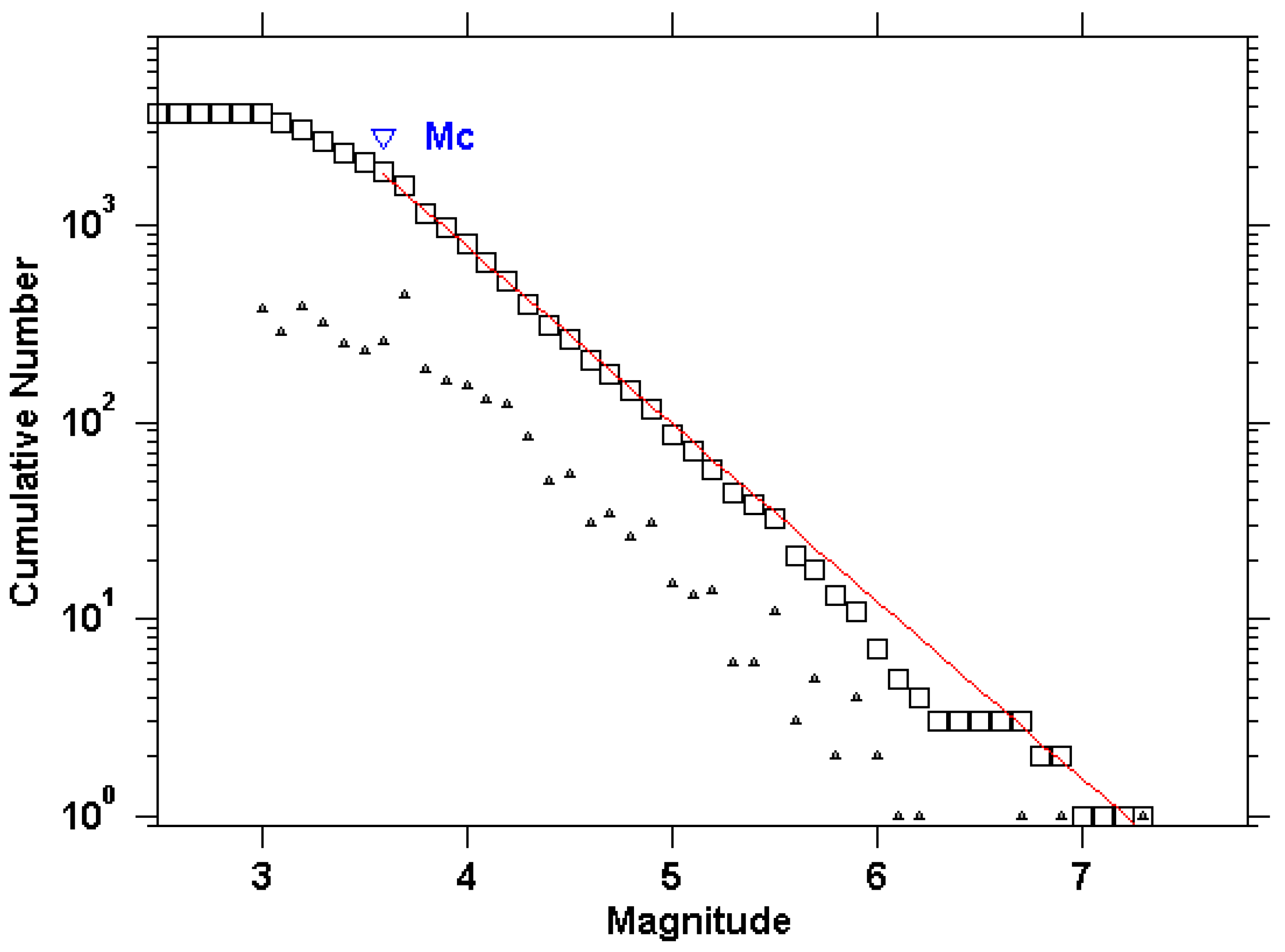
4.1. Earthquake Catalogue of Northern Algeria and Its Vicinity

The seismic events that occurred in Northern Algeria and its vicinity, during the period 1950–2021 and within the region between latitudes 32–38° and longitudes −2–10°, were studied in this article (Figure 1). The reported earthquakes mostly occurred along the active faults of the Tell Atlas belt, the most active seismic zone in Northern Algeria [60]. Its seismic activity is strongly related to the convergence between the African and the Eurasian plates (e.g., [61,62]). The catalogue used in this study was compiled by integrating information from various sources, starting from published papers [63,64,65] and including data available from the International Seismological Centre, ISC (http://isc.ac.uk/; last accessed on 27 December 2021) and from the European–Mediterranean Seismological Centre, EMSC (https://www.emsc-csem.org/#2; last accessed on 27 December 2021). The considered area comprises the largest and the most damaging earthquakes ever recorded in the Mediterranean region, such as the M7.3 (El Asnam, 1980), M6.9 (Boumerdes, 2003), and M6.7 (El Asnam, 1954) earthquakes. Namely, the M7.3 (El Asnam, 1980) earthquake was located near the Oued Fodda village, the M6.7 (El Asnam, 1954) earthquake was positioned near Beni Rached in the northeast of Orléansville, and the M6.9 (Boumerdes, 2003) earthquake was located near the coastal village of Zemmouri (Figure 1) [62].

Figure 2 shows the variations of the completeness magnitude $M_c$ with time which was calculated via the Maximum Curvature (MAXC) method [41], while Figure 3 shows the magnitude of completeness $M_c=3.6$ which was calculated using the best among 95% probability and 90% probability MAXC method implemented by ZMAP [42]. In addition, we estimated the completeness magnitude by different methods such as the Entire Magnitude Range (EMR) method [66,67], the $b$–value stability (MBS) method [68], and the Goodness-of-Fit Test (GFT) [41], and we found values between $3.5$ and $3.6$. Additionally, we estimated the magnitude $M_c$ for different time spans, e.g., 1950–1998 and 1998–2021, and we found stable values around 3.6. Ultimately, the completeness magnitude $M_c=3.7$ was found to be a conservative completeness estimate according to those methods and time spans. Despite possible spatial issues in data completeness, it seems that for $M_c=3.7$, there should be no significant border effects, as the most active areas were located well inside the study region. Figure 1 illustrates the spatial distribution of the Northern Algerian seismicity, with 1561 events of magnitude at least $3.7$, which were mostly concentrated in the Mediterranean region [69].

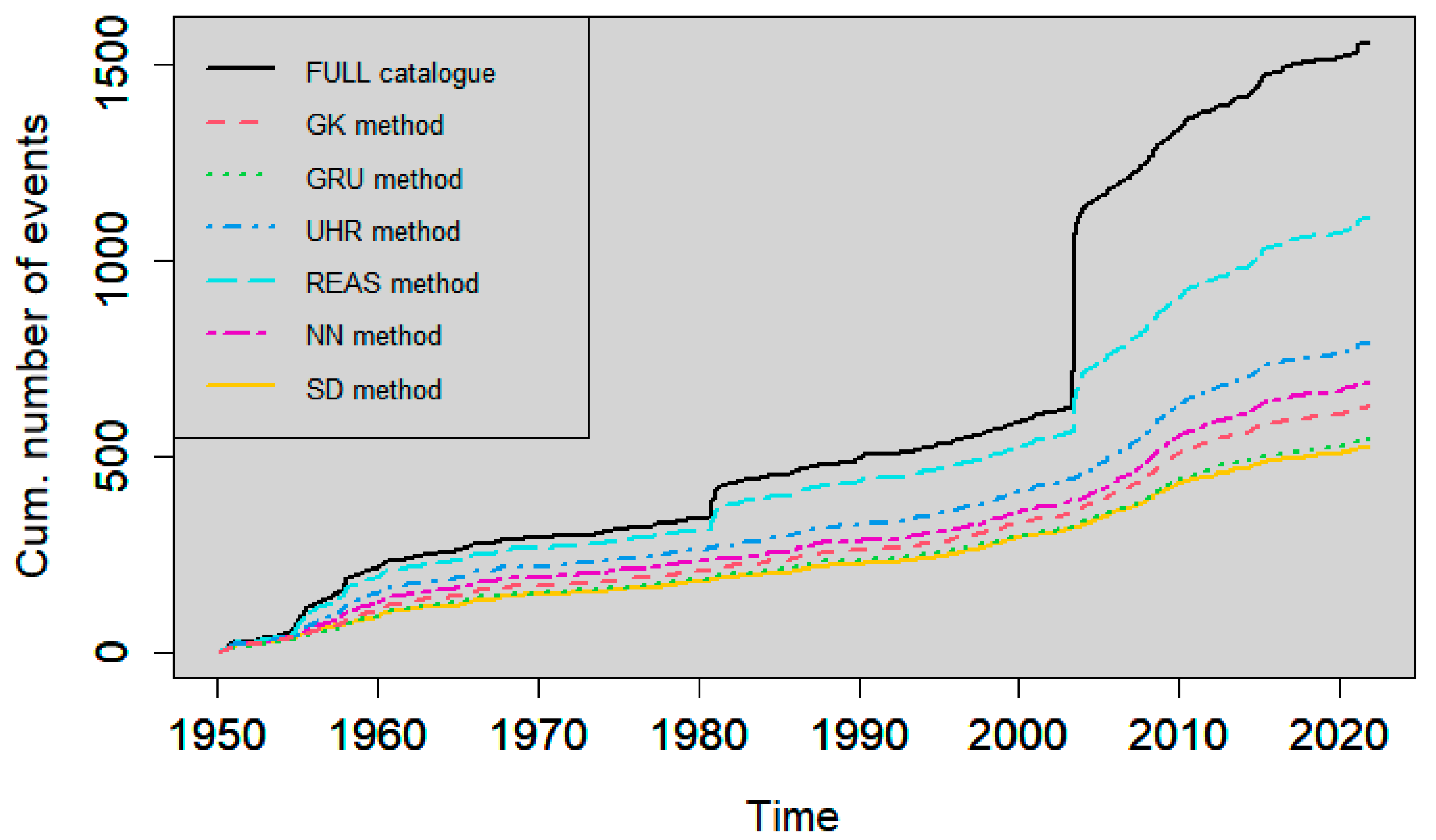
4.2. Declustering Application

In this article, the declustering algorithms presented in Section 2 were applied to the Northern Algerian earthquakes catalogue. The used parameterization of the windowing and cluster methods have already been explained, except for the SD and NN methods. Specifically, the SD algorithm application necessitates the estimation of the ETAS parameters [5,6,31]. In this case, the final MLE values of the ETAS model used to fit the study region were $\widehat{\nu }=1.02$, $\widehat{A}=0.56$, $\widehat{c}=0.01$, $\widehat{\alpha }=1.02$, $\widehat{p}=1.09$, $\widehat{D}=0.005$, $\widehat{q}=2.02$, and $\widehat{\gamma }=0.39$. By denoting the catalogue period by $\left[0,T\right]$, the corresponding plots of the estimated background seismicity rate $\widehat{\mu }\left(x,y\right)$, the total spatial seismicity rate $\widehat{\mathsf{\Lambda }}\left(x,y\right)=T^{-1}{{\displaystyle \int }}_0^T\widehat{\lambda }\left(t,x,y\right)dt$, the clustering coefficient $1-\widehat{\mu }\left(x,y\right)/\widehat{\mathsf{\Lambda }}\left(x,y\right)$, and the conditional intensity at the end of the study period $\widehat{\lambda }\left(T,x,y\right)$ are presented in Figure 4 (see [70] for more details about the rates and coefficient forms, as well as [5,6]). As expected, the estimated background seismicity rate was high around locations of large earthquakes close to the Algerian coast, specifically the recent M5.4 (Béjaia, 2021), M6.9 (Boumerdes, 2003), and M7.3 (El Asnam, 1980) earthquakes, and less high elsewhere. The clustering coefficient, which estimates the aftershocks triggering in given longitude–latitude coordinates, was highly significant in many areas around the main seismic faults. The total spatial seismicity rate appeared distributed almost uniformly along the Algerian coast with exception of the Boumerdes earthquake location and its vicinity, which showed a significantly high value. In other words, it showed a less intense seismic activity with small clusters distribution in the high plateaus and the Saharan Atlas, contrary to the Tell Atlas. The input parameters of the NN method were estimated to $\widehat{b}=0.99$ and ${\widehat{d}}_f=0.81$ using the ZMAP software [42], and the threshold distance ${\eta }_0$ is calculated using the criterion of the mixture of two Gaussian distributions, i.e., ${\log }_{10}{\widehat{\eta }}_0=-5.5$, as it is shown in Figure 5.

The resulting background seismicity after declustering included 630, 548, 794, 1110, 692, and 526 events based on GK, GRU, UHR, REAS, NN, and SD methods, respectively, which correspond to 40.35%, 35.10%, 50.86%, 71.10%, 44.33%, and 33.69% of the earthquakes reported in the catalogue. The longitude versus time is shown for the full catalogue in Figure 6, and for each declustered catalogue in Figure 7, Figure 8, Figure 9, Figure 10, Figure 11 and Figure 12. The red circles in these figures highlight the presence of clusters, which were characterised by a strong spatiotemporal closeness of the earthquakes. Figure 13 compares the full and the declustered catalogues in terms of the cumulative number of events versus time. It shows that the REAS method detected a fewer number of dependent (clustered) earthquakes compared to the other declustering methods, because the corresponding graph was the closest to the full catalogue graph and the farthest from the expected linear trend of a time-homogeneous Poisson process. This outcome signifies that the REAS method failed someway to totally eliminate the clustering behaviour from the full catalogue. It was also observed that GRU and SD methods were the most successful in reducing the space–time clustering in Northern Algerian seismicity. We highlight the sharp increase in the cumulative number of events in the full catalogue after major earthquakes, particularly after the 2003 Boumerdes earthquake. The increase can be explained by the enhanced seismic activity (foreshocks and aftershocks) associated with large events, and can be also partially due to the improvements in the seismic monitoring network in the region since 2003 Boumerdes earthquake, resulting in the locally increased detection capability of events [71]. The GRU and SD methods seem to be able to better remove the clustering than the other methods; the sharp increase was not evident in the corresponding declustered catalogues in Figure 13. These results are further investigated in the next section by carrying out rigorous statistical analysis.

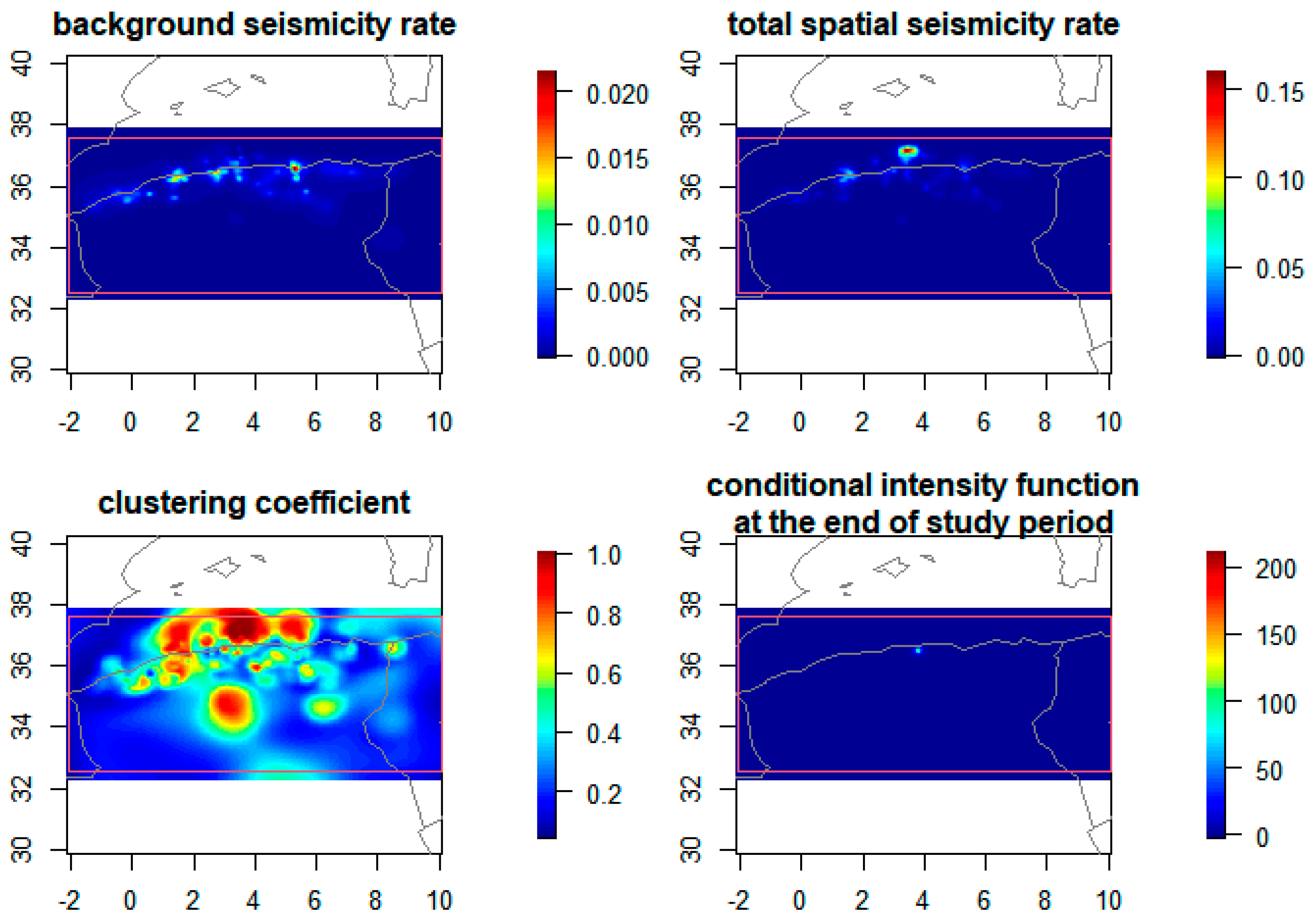
4.3. Spatiotemporal Analysis of the Declustered Catalogues

The obtained declustered catalogues were compared on the basis of different space–time empirical measures to assess if the space–time clustering was still present after declustering, and to test the hypothesis according to which a declustered catalogue follows a temporally homogeneous and spatially inhomogeneous Poisson process. First, we analysed and compare the behaviour of the background occurrence times of the six declustered catalogues. Namely, CV was used to assess the clustering behaviour, without any information about the timescale ranges where the process was clearly clustered, including the empirical measure given by Equation (13). The AF was then used for assessing and measuring the time correlation in the resulting background seismicity. The MMPP was used to study the temporal changes in the background seismicity rate.

A fast and simple assessment of the time-homogeneous Poisson hypothesis was from the CV measure in Equation (12), which was calculated for all declustered catalogues (

Table 2. CV values of all declustered catalogues.

Method	GK	GRU	UHR	REAS	NN	SD
CV	1.50	1.40	1.68	2.06	1.57	1.35

). The obtained values exceeded unity, which means a possible existence of clustering behaviour. Typically, a CV value much higher than $1$ implies that relevant clustered earthquake patterns are still present in the declustered catalogues; for example, the REAS declustered catalogue showed more clustering than others. However, additional statistical tests are needed to assess if the obtained CV values are significantly different from unity. According to Equation (13), Figure 14 illustrates the $Y\left(t\right)$ plots for all declustered catalogues, accompanied by their corresponding 95% envelopes from Monte Carlo simulations; it shows that none of the declustered catalogues were completely Poissonian at all timescales. However, we can observe that GRU and SD methods performed better than the other methods, which displayed a significant deviation from the theoretical Poisson process and the simulation envelopes.

For each declustered catalogue Figure 15 displays, on a log–log scale, its AF curve (black solid line) as well as the theoretical Poisson process (green dashed line) and the 95% confidence band (grey band) obtained from the Monte Carlo simulation of a time-homogeneous Poisson process having same rate and event number of the original declustered catalogue. Except for the REAS method, the AF plots of the declustered catalogues are almost flat around zero, showing likely Poissonian behaviours at a short timescale. A departure from the Poisson distribution appeared at timescales greater than 2.9, 2.5, 3, and 2.2, which correspond approximately to 794, 316, 1000, and 158 days, for GRU, GK, SD, and NN methods, respectively. These cut-off timescales, also called fractal onset times, indicate the lowest timescale from which the clustering behaviour appears. The highest of these values come from the GRU and SD methods, which means that GRU and SD methods produce catalogues of events that result not significantly correlated in time at both short and intermediate timescales, and, consequently, are closer to Poissonian behaviour than GK and NN. Since the AF curve in the log–log scale has a linear trend at long as well as intermediate timescales, a power–law function for the counting time $\tau$ was suggested.

The temporal evolution of the background seismicity rate, as provided by each declustered catalogue, was further investigated by applying different $K$–MMPP models, $K\ge 1$, in order to identify possible variations over time.

Table 3. Estimated Poisson rates, maximum log-likelihood values, and BICs for K–MMPPs best fitting models to the declustered catalogues.

Declustering Method	K-MMPP Model	Poisson Rate	Maximum Log–Likelihood	BIC
GK	2-MMPP	$$\begin{gathered} {\widehat{\lambda }}_1=0.045 \\ {\widehat{\lambda }}_2=0.014 \end{gathered}$$	$-2896.007$	$5817.797$
GRU	2-MMPP	$$\begin{gathered} {\widehat{\lambda }}_1=0.037 \\ {\widehat{\lambda }}_2=0.013 \end{gathered}$$	$-2611.608$	$5248.442$
UHR	4-MMPP	$$\begin{gathered} {\widehat{\lambda }}_1=379.775 \\ {\widehat{\lambda }}_2=1.953 \\ {\widehat{\lambda }}_3=0.052 \\ {\widehat{\lambda }}_4=0.007 \end{gathered}$$	$-3362.443$	$6831.720$
REAS	5-MMPP	$$\begin{gathered} {\widehat{\lambda }}_1=2008.041 \\ {\widehat{\lambda }}_2=1.682 \\ {\widehat{\lambda }}_3=0.253 \\ {\widehat{\lambda }}_4=0.054 \\ {\widehat{\lambda }}_5=0.011 \end{gathered}$$	$-3896.425$	$7968.153$
NN	2-MMPP	$$\begin{gathered} {\widehat{\lambda }}_1=0.055 \\ {\widehat{\lambda }}_2=0.014 \end{gathered}$$	$-3097.183$	$6220.525$
SD	2-MMPP	$$\begin{gathered} {\widehat{\lambda }}_1=0.033 \\ {\widehat{\lambda }}_2=0.011 \end{gathered}$$	$-2528.608$	$5082.277$

contains the estimated Poisson rates for $K$–MMPPs best fitting models, the associated maximum log-likelihood values, and BICs. According to BIC, the MMPP models with $K=2, 2, 4, 5, 2, 2$ states are the best models among the aforementioned competing models that fit the declustered catalogues identified by GK, GRU, UHR, REAS, NN, and SD methods, respectively.

A switched Poisson process with multiple states (i.e., a $K$–MMPP model with $K>1$) is hence the best model for describing the background seismicity process in all methods. Figure 16 refers to the GK declustered catalogue and its best estimated $K$–MMPP, $K=2$; the figure shows the estimated smoothing probabilities $P(X\left(t_j\right)=s |t_1,t_2,\dots ,t_n)$ of each state $s\in S=\left\{1, 2,\dots ,K\right\}$, for all occurrence times $\left\{t_j: j=1,\dots ,n\right\}$ of the background events. Similarly, Figure 17, Figure 18, Figure 19, Figure 20 and Figure 21 refer to the GRU, UHR, REAS, NN, and SD declustered catalogues and their best estimated $K$–MMPPs, respectively. The $K$ states of the MMPP models are represented by different colours: state 1 in red, state 2 in blue, state 3 in green, state 4 in magenta, and state 5 in orange. Based on Figure 16, Figure 17, Figure 18, Figure 19, Figure 20 and Figure 21, the states 1, 1, 3, 4, 1, and 1 each correspond to the estimated Poisson rates ${\widehat{\lambda }}_1=0.045$, ${\widehat{\lambda }}_1=0.037$, ${\widehat{\lambda }}_3=0.052$, ${\widehat{\lambda }}_4=0.054$, ${\widehat{\lambda }}_1=0.055$, ${\widehat{\lambda }}_1=0.033$ and are each the most probable states for 60.47%, 54.74%, 59.69%, 44.32%, 60.83%, and 68.63% of the events in the background earthquake catalogues identified by GR, GRU, UHR, REAS, NN, and SD methods, respectively. The highest Poisson rates found in the cases of REAS and UHR background seismicity (${\widehat{\lambda }}_1=2008.041$ and ${\widehat{\lambda }}_1=379.775$) were probably due to those clustered events misclassified by the two methods in the declustered catalogues. Additionally, a significant switch between one state to another state, which is expressed by the transition from one Poisson rate value to a higher Poisson rate value, is often detected in case of large earthquake occurrences (e.g., after 1954 and 2003 events) in Northern Algeria and its vicinity.

The spatial analysis of the six background earthquake catalogues was performed by using MI and the inhomogeneous version of L-function, respectively given in Equations (18) and (20), to assess and measure the possible presence of spatial clustering. Figure 22 shows the linear regression fitting of ${\log }_{10}{I}_{\delta }$ and ${\log }_{10} \delta$, where $I_{\delta }$ is the value of MI for a spatial grid having cell size $\delta$. A significant departure in the logarithm of the MI curves from 0 (i.e., a departure of $I_{\delta }$ from $1$) denotes the existence of clustered dynamics in the spatial patterns of Northern Algeria and the surrounding areas. Based on the slope $S_2$ defined by Equation (19), the highest clustering degree was shown by the REAS method while the smallest was shown by the GRU method. Specifically, these slopes are calculated by the least square method (

Table 4. Calculated MI slopes for full and declustered catalogues.

Declustering Method	Full Catalogue	GK	GRU	UHR	REAS	NN	SD
${\mathit{S}}_{\mathbf{2}}$	0.49	0.31	0.29	0.34	0.37	0.33	0.32

). Clearly, all the considered methods of declustering reduced the spatial clustering, but did not totally eliminate it because seismicity tends to develop naturally along the fault systems.

Figure 23 illustrates the results of the inhomogeneous version of the L-function for the six declustered catalogues: the null hypothesis of spatially inhomogeneous Poisson process was rejected at the 5% significance level for all declustered catalogues. Moreover, all the empirical plots of the L-function deviated upward outside the 95% confidence zone, i.e., $L\left(r\right)>r$, at slightly different intervals of the spatial distance, thus providing further evidence of spatial clustering. On the contrary, downward deviations ($L\left(r\right)<r$), which denote the existence of a negative pairwise correlation, were essentially not observed.

5. Conclusions

In this article, we provided new insights into the problem of identifying and quantifying the time-correlation and the space-clustering in the background earthquake catalogues identified by different declustering methods, specifically GK, GRU, UHR, REAS, NN, and SD methods. We applied different spatiotemporal measures, namely the CV, AF, and MMPP were used for assessing temporal clustering, while the MI and inhomogeneous L-function were used for a space clustering study in the Northern Algerian area and its vicinity. Our results showed that the declustering methods reduced the time of correlation structures in the declustered catalogues at small timescales, but temporal correlation still remains at intermediate and higher timescale ranges. The performances of the GRU and SD methods seem to be preferable in terms of removing the time clustering structures; in fact, the cut-off timescale was higher for these methods than the others. In all cases, the switched Poisson process with multiple states proved to be the best model which could describe background seismicity in time, even for GRU and SD declustered catalogues. Moreover, for all declustered catalogues, the spatially inhomogeneous Poisson process did not fit properly the spatial distribution of earthquake epicentres. The results showed that the spatial clustering structure was significantly reduced, but it was not eliminated from the declustered catalogues, due to the natural clustering of seismicity along existing fault systems. Hence, the assumption of stationary and homogeneous Poisson process, widely used in seismic hazard assessment, was not met by the investigated catalogue, independently from the adopted declustering method. Accounting for the spatiotemporal features of the background seismicity identified in this study is, therefore, a key element towards effective seismic hazard assessment and earthquake forecasting in Algeria and the surrounding area.

References

1. Aki, K. Some Problems in Statistical Seismology. Zisin 1956, 8, 205–228. [Google Scholar] [CrossRef] [PubMed] [Green Version]
2. Kagan, Y.; Jackson, D. Long–term earthquake clustering. Geophys. J. Int. 1991, 104, 117–133. [Google Scholar] [CrossRef] [Green Version]
3. Ogata, Y. Statistical models for earthquake occurrences and residual analysis for point processes. J. Am. Stat. Assoc. 1988, 83, 9–27. [Google Scholar] [CrossRef]
4. Ogata, Y. Space–time point process models for earthquake occurrences. Ann. Inst. Stat. Math. 1998, 50, 379–402. [Google Scholar] [CrossRef]
5. Zhuang, J.; Ogata, Y.; Vere–Jones, D. Stochastic declustering of space–time earthquake occurrences. J. Am. Stat. Assoc. 2002, 97, 369–380. [Google Scholar] [CrossRef]
6. Zhuang, J.; Ogata, Y.; Vere–Jones, D. Analyzing earthquake clustering features by using stochastic reconstruction. J. Geophys. Res. 2004, 109, B05301. [Google Scholar] [CrossRef] [Green Version]
7. Zhuang, J.; Murru, M.; Falcone, G.; Guo, Y. An extensive study of clustering features of seismicity in Italy from 2005 to 2016. Geophys. J. Int. 2019, 216, 302–318. [Google Scholar] [CrossRef]
8. Zaliapin, I.; Ben–Zion, Y. Earthquake clusters in southern California I: Identification and stability. J. Geophys. Res. Solid Earth 2013, 118, 2847–2864. [Google Scholar] [CrossRef]
9. Zaliapin, I.; Ben–Zion, Y. A global classification and characterization of earthquake clusters. Geophys. J. Int. 2016, 207, 608–634. [Google Scholar] [CrossRef] [Green Version]
10. Zaliapin, I.; Ben–Zion, Y. Earthquake declustering using the nearest–neighbor approach in space–time–magnitude domain. J. Geophys. Res. Solid Earth 2020, 125, e2018JB017120. [Google Scholar] [CrossRef]
11. Benali, A.; Peresan, A.; Varini, E.; Talbi, A. Modelling background seismicity components identified by nearest neighbour and stochastic declustering approaches: The case of Northeastern Italy. Stoch. Environ. Res. Risk Assess. 2020, 34, 775–791. [Google Scholar] [CrossRef]
12. Benali, A.; Zhuang, J.; Talbi, A. An updated version of the ETAS model based on multiple change points detection. Acta Geophys. 2022, 70, 2013–2031. [Google Scholar] [CrossRef]
13. Varotsos, P.A.; Sarlis, N.V.; Skordas, E.S.; Uyeda, S.; Kamogawa, M. Natural-time analysis of critical phenomena: The case of seismicity. Europhys. Lett. 2010, 92, 29002. [Google Scholar] [CrossRef] [Green Version]
14. Sarlis, N.V.; Skordas, E.S.; Varotsos, P.A.; Nagao, T.; Kamogawa, M.; Uyeda, S. Spatiotemporal variations of seismicity before major earthquakes in the Japanese area and their relation with the epicentral locations. Proc. Natl. Acad. Sci. USA 2015, 112, 986–989. [Google Scholar] [CrossRef] [Green Version]
15. Rundle, J.B.; Turcotte, D.L.; Donnellan, A.; Grant Ludwig, L.; Luginbuhl, M.; Gong, G. Nowcasting earthquakes. Earth Space Sci. 2016, 3, 480–486. [Google Scholar] [CrossRef]
16. Varotsos, P.K.; Perez-Oregon, J.; Skordas, E.S.; Sarlis, N.V. Estimating the Epicenter of an Impending Strong Earthquake by Combining the Seismicity Order Parameter Variability Analysis with Earthquake Networks and Nowcasting: Application in the Eastern Mediterranean. Appl. Sci. 2021, 11, 10093. [Google Scholar] [CrossRef]
17. Perez-Oregon, J.; Varotsos, P.K.; Skordas, E.S.; Sarlis, N.V. Estimating the epicenter of a Future Strong Earthquake in Southern California, Mexico and Central America by means of Natural Time Analysis and earthquake Nowcasting. Entropy 2021, 23, 1658. [Google Scholar] [CrossRef]
18. van Stiphout, T.; Zhuang, J.; Marsan, D. Seismicity Declustering. Community Online Resource for Statistical Seismicity Analysis. 2012, pp. 1–25. Available online: http://www.corssa.org (accessed on 1 September 2022). [CrossRef]
19. Nas, M.; Jalilian, A.; Bayrak, Y. Spatiotemporal comparison of declustered catalogs of earthquakes in Turkey. Pure Appl. Geophys. 2019, 176, 2215–2233. [Google Scholar] [CrossRef]
20. Talbi, A.; Nanjo, K.; Satake, K.; Zhuang, J.; Hamdache, M. Comparison of seismicity declustering methods using a probabilistic measure of clustering. J. Seismol. 2013, 17, 1041–1061. [Google Scholar] [CrossRef]
21. Telesca, L.; Lovallo, M.; Golay, J.; Kanevski, M. Comparing seismicity declustering techniques by means of the joint use of Allan Factor and Morisita index. Stoch. Environ. Res. Risk Assess. 2015, 30, 77–90. [Google Scholar] [CrossRef]
22. Touati, S.; Naylor, M.; Main, I. Detection of change points in underlying earthquake rates, with application to global mega earthquakes. Geophys. J. Int. 2016, 204, 753–767. [Google Scholar] [CrossRef]
23. Gardner, J.K.; Knopoff, L. Is the sequence of earthquakes in Southern California, with aftershocks removed, Poissonian? Bull. Seismol. Soc. Am. 1974, 64, 1363–1367. [Google Scholar] [CrossRef]
24. Uhrhammer, R. Characteristics of northern and central California seismicity. Earthq. Notes 1986, 57, 21. [Google Scholar]
25. Luen, B.; Stark, P.B. Poisson tests of declustered catalogues. Geophys. J. Int. 2012, 189, 691–700. [Google Scholar] [CrossRef] [Green Version]
26. Kolev, A.A.; Ross, G.J. Inference for etas models with non–poissonian mainshock arrival times. Stat. Comput. 2019, 29, 915–931. [Google Scholar] [CrossRef] [Green Version]
27. Li, C.; Song, Z.; Wang, W. Space–time inhomogeneous background intensity estimators for semi parametric space–time self–exciting point process models. Ann. Inst. Stat. Math. 2019, 72, 945–967. [Google Scholar] [CrossRef]
28. Baiesi, M.; Paczuski, M. Scale-free networks of earthquakes and aftershocks. Phys. Rev. E 2004, 69, 066106. [Google Scholar] [CrossRef] [Green Version]
29. Bountzis, P.; Kostoglou, A.; Papadimitriou, E.; Karakostas, V. Identification of spatiotemporal seismicity clusters in central Ionian Islands (Greece). Phys. Earth Planet. Inter. 2021, 312, 106675. [Google Scholar] [CrossRef]
30. Reasenberg, P. Second-order moment of central California seismicity, 1969–1982. J. Geophys. Res. 1985, 90, 5479–5495. [Google Scholar] [CrossRef]
31. Zhuang, J. Second-order residual analysis of spatiotemporal point processes and applications in model evaluation. J. R. Stat. Soc. Ser. B 2006, 68, 635–653. [Google Scholar] [CrossRef]
32. Teng, G.; Baker, J.W. Seismicity Declustering and Hazard Analysis of the Oklahoma-Kansas Region. Bull. Seismol. Soc. Am. 2019, 109, 2356–2366. [Google Scholar] [CrossRef]
33. Allan, D.W. Statistics of atomic frequency standards. Proc. IEEE 1966, 54, 221–230. [Google Scholar] [CrossRef] [Green Version]
34. Morisita, M. Measuring of the dispersion of individuals and analysis of the distributional patterns. Mem. Fac. Sci. Kyushu Univ. Ser. E 1959, 2, 215–235. [Google Scholar]
35. Telesca, L.; Cuomo, V.; Lapenna, V.; Macchiato, M. On the methods to identify clustering properties in sequences of seismic time-occurrences. J. Seismol. 2002, 6, 125–134. [Google Scholar] [CrossRef] [Green Version]
36. Besio, G.; Briganti, R.; Romano, A.; Mentaschi, L.; De Girolamo, P. Time clustering of wave storms in the Mediterranean Sea. Nat. Hazards Earth Syst. Sci. 2017, 17, 505–514. [Google Scholar] [CrossRef] [Green Version]
37. Telesca, L.; Kanevski, M.; Tonini, M.; Pezzatti, G.B.; Conedera, M. Temporal patterns of fire sequences observed in Canton of Ticino (southern Switzerland). Nat. Hazards Earth Syst. Sci. 2010, 10, 723–728. [Google Scholar] [CrossRef] [Green Version]
38. Yip, C.F.; Ng, W.L.; Yau, C.Y. A hidden Markov model for earthquake prediction. Stoch. Environ. Res. Risk Assess. 2018, 32, 1415–1434. [Google Scholar] [CrossRef]
39. Lu, S. A Bayesian multiple changepoint model for marked Poisson processes with applications to deep earthquakes. Stoch. Environ. Res. Risk Assess. 2019, 33, 59–72. [Google Scholar] [CrossRef]
40. Peresan, A.; Gentili, S. Identification and characterization of earthquake clusters: A comparative analysis for selected sequences in Italy and adjacent regions. Boll. Di Geofis. Teor. E Appl. 2020, 61, 57–80. [Google Scholar] [CrossRef]
41. Wiemer, S.; Wyss, M. Minimum magnitude of completeness in earthquake catalogs: Examples from Alaska, the western United States, and Japan. Bull. Seismol. Soc. Am. 2000, 90, 859–869. [Google Scholar] [CrossRef]
42. Wiemer, S. A software package to analyze seismicity: ZMAP. Seismol. Res. Lett. 2001, 72, 373–382. [Google Scholar] [CrossRef]
43. Omori, F. Investigation of aftershocks. Rep. Earthq. Inv. Comm. 1894, 2, 103–139. [Google Scholar]
44. Zaliapin, I.; Gabrielov, A.; Wong, H.; Keilis-Borok, V.I. Clustering analysis of seismicity and aftershock identification. Phys. Rev. Lett. 2008, 101, 018501. [Google Scholar] [CrossRef] [Green Version]
45. Papadopoulou, K.A.; Skordas, E.S.; Sarlis, N.V. A tentative model for the explanation of Båth law using the order parameter of seismicity in natural time. Earthq. Sci. 2016, 29, 311–319. [Google Scholar] [CrossRef] [Green Version]
46. Gutenberg, B.; Richter, C.F. Frequency of earthquakes in California. Bull. Seismol. Soc. Am. 1944, 34, 185–188. [Google Scholar] [CrossRef]
47. Nekrasova, A.; Kossobokov, V.; Peresan, A.; Aoudia, A.; Panza, G.F. A multiscale application of the unified scaling law for earthquakes in the central Mediterranean area and alpine region. Pure Appl. Geophys. 2011, 168, 297–327. [Google Scholar] [CrossRef]
48. Bottiglieri, M.; Lippiello, E.; Godano, C.; de Arcangelis, L. Identification and spatiotemporal organization of aftershocks. J. Geophys. Res. 2009, 114, B03303. [Google Scholar] [CrossRef]
49. Telesca, L.; Cuomo, V.; Lapenna, V.; Macchiato, M. Analysis of the time-scaling behaviour in the sequence of the aftershocks of the Bovec (Slovenia) April 12, 1998 earthquake. Phys. Earth Planet Int. 2000, 120, 315–326. [Google Scholar] [CrossRef]
50. Cox, D.R.; Isham, V. Point Processes; Chapman and Hall: London, UK, 1980. [Google Scholar]
51. Telesca, L.; Lovallo, M.; Amin Mohamed, A.E.E.; ElGabry, M.; El-hady, S.; Abou Elenean, K.M.; ElShafey Fat ElBary, R. Investigating the time-scaling behavior of the 2004–2010 seismicity of Aswan area (Egypt) by means of the Allan factor statistics and the detrended fluctuation analysis. Nat. Hazards Earth Syst. Sci. 2012, 12, 1267–1276. [Google Scholar] [CrossRef] [Green Version]
52. Telesca, L.; Bernardi, M.; Rovelli, C. Time-scaling analysis of lightning in Italy. Commun. Nonlinear Anal. Numer. Simul. 2008, 13, 1384–1396. [Google Scholar] [CrossRef]
53. Rydén, T. Parameter estimation for Markov modulated Poisson processes. Commun. Stat. Stoch. Model. 1994, 10, 795–829. [Google Scholar] [CrossRef]
54. Rydén, T. An EM algorithm for estimation in Markov-modulated Poisson processes. Comput. Stat. Data Anal. 1996, 21, 431–447. [Google Scholar] [CrossRef]
55. Harte, D. HiddenMarkov: Hidden Markov Models R Package Version 1.8-11; Statistics Research Associates: Wellington, New Zealand, 2017; Available online: http://www.statsresearch.co.nz/dsh/sslib/ (accessed on 11 July 2022).
56. Kass, R.E.; Raftery, A.E. Bayes factors. J. Am. Stat. Assoc. 1995, 90, 773–795. [Google Scholar] [CrossRef]
57. Hayes, J.J.; Castillo, O. A new approach for interpreting the Morisita index of aggregation through quadrat size. ISPRS Int. J. Geo-Inf. 2017, 6, 296. [Google Scholar] [CrossRef]
58. Morisita, M. Iδ-index, a measure of dispersion of individuals. Res. Popul. Ecol. 1962, 4, 1–7. [Google Scholar] [CrossRef]
59. Besag, J.E. Contribution to the discussion on Dr. Ripley’s Paper. J. R. Stat. Soc. Ser. B 1977, 39, 193–195. [Google Scholar]
60. Bezzeghoud, M.; Ayadi, A.; Caldeira, B.; Fontiela, J.; Borges, J.F. The largest earthquakes in Algeria in the modern period: The El Asnam and Zemmouri Boumerdès faults. Física De La Tierra 2017, 29, 183–202. [Google Scholar] [CrossRef] [Green Version]
61. Meghraoui, M. Géologie des Zones Sismiques du Nord de l’Algérie, Paléosismologie, Tectonique Active et Synthèse Sismotectonique. Ph.D. Thesis, Université Paris, Paris, France, 1988; p. 356. [Google Scholar]
62. Yelles–Chaouche, A.; Kherroubi, A.; Beldjoudi, H. The large Algerian earthquakes (267 A.D.–2017). Física De La Tierra 2017, 29, 159–182. [Google Scholar] [CrossRef] [Green Version]
63. Benouar, D. An earthquake catalogue for the Maghreb region 20°–38° N, 10° W–12° E for the period 1900–1990. Ann. Geofis. 1994, 37, 511–528. [Google Scholar]
64. Harbi, A.; Peresan, A.; Panza, G.F. Seismicity of Eastern Algeria: A revised and extended earthquake Catalogue. Nat. Hazards 2010, 54, 725–747. [Google Scholar] [CrossRef]
65. Ayadi, A.; Bezzeghoud, M. Seismicity of Algeria from 1365 to 2013: Maximum observed intensity map (MOI2014). Seismol. Res. Lett. 2015, 86, 236–244. [Google Scholar] [CrossRef] [Green Version]
66. Ogata, Y.; Katsura, K. Analysis of temporal and spatial heterogeneity of magnitude frequency distribution inferred from earthquake catalogues. Geophys. J. Int. 1993, 113, 727–738. [Google Scholar] [CrossRef] [Green Version]
67. Woessner, J.; Wiemer, S. Assessing the quality of earthquake catalogues: Estimating the magnitude of completeness and its uncertainty. Bull. Seismol. Soc. Am. 2005, 95, 684–698. [Google Scholar] [CrossRef]
68. Cao, A.M.; Gao, S.S. Temporal variations of seismic b-values beneath northeastern Japan island arc. Geophys. Res. Lett. 2002, 29, 1334. [Google Scholar] [CrossRef]
69. Idrissou, S.; (Département de Génie Civil, Faculté de Technologie, Université Abderrahmane Mira, Béjaia, Algeria). Personal communication, 2023.
70. Jalilian, A. ETAS: An R package for fitting the space-time ETAS model to earthquake data. J. Stat. Softw. 2019, 88, 1–39. [Google Scholar] [CrossRef] [Green Version]
71. Yelles-Chaouche, A.; Allili, T.; Alili, A.; Messemen, W.; Beldjoudi, H.; Semmane, F.; Kherroubi, A.; Djellit, H.; Larbes, Y.; Haned, S.; et al. The new Algerian Digital Seismic Network (ADSN): Towards an earthquake early-warning system. Adv. Geosci. 2013, 36, 31–38. [Google Scholar] [CrossRef] [Green Version]
Figure 1. Spatial distribution of the Northern Algerian epicentres for 1561 earthquakes with magnitude M 3.7 within the time period 1950–2021.
Axioms 12 00237 g001
Figure 2. Estimated magnitude of completeness M c as a function of time, calculated using MAXC technique in ZMAP with the sample window size of 100, the binning of 0.1, and 200 bootstrap samples as standard parameters for the error bounds, presented as red dashed lines.
Axioms 12 00237 g002
Figure 3. Fitted Frequency–Magnitude Distribution (FMD) is used to calculate the magnitude of completeness M c = 3.6 , the squares and the triangles indicate the cumulative and non-cumulative FMD, respectively, and the red line represents the fitted G–R law for b ^ = 0.903 and a ^ = 6.51 .
Axioms 12 00237 g003
Figure 4. Plots of the estimated background seismicity rate, clustering coefficient, total spatial seismicity rate, and conditional intensity at the end of the study time period for the Northern Algerian catalogue.
Axioms 12 00237 g004
Figure 5. (a) 1−D density distribution of log 10   η , where the estimated Gaussian densities for clustered and background seismicity classes are labelled by blue and red colours, respectively; (b) 2−D distribution of rescaled space and rescaled time distances.
Axioms 12 00237 g005
Figure 6. Longitude versus time of the full earthquake catalogue. Red circles highlight the presence of clustering behaviour.
Axioms 12 00237 g006
Figure 7. Longitude versus time of the GK declustered catalogue. Red circles highlight the presence of clustering behaviour.
Axioms 12 00237 g007
Figure 8. Longitude versus time of the GRU declustered catalogue.
Axioms 12 00237 g008
Figure 9. Longitude versus time of the UHR declustered catalogue. Red circles highlight the presence of clustering behaviour.
Axioms 12 00237 g009
Figure 10. Longitude versus time of the REAS declustered catalogue. Red circles highlight the presence of clustering behaviour.
Axioms 12 00237 g010
Figure 11. Longitude versus time of the NN declustered catalogue. Red circles highlight the presence of clustering behaviour.
Axioms 12 00237 g011
Figure 12. Longitude versus time of the SD declustered catalogue.
Axioms 12 00237 g012
Figure 13. Cumulative number of earthquakes with M 3.7 in the full catalogue compared to the declustered catalogues.
Axioms 12 00237 g013
Figure 14. Observed, theoretical Poisson, and 95% confidence bands of Y t given in Equation (13) for all declustered catalogues, represented by black solid line, green dashed line, and grey band, respectively. The unit of time is in days.
Axioms 12 00237 g014
Figure 15. Log–log scales plots of AF measure for the residual declustered catalogues. Observed, theoretical Poisson, and 95% confidence area of this measure are shown by the black solid line, green dashed line, and grey band, respectively. The unit of time is in days.
Axioms 12 00237 g015
Figure 16. States probabilities associated with each background occurrence time for the 2-MMPP model that best fits the declustered catalogue obtained by the GK method. Red and blue colours are assigned to states 1 and 2, respectively. Grey vertical dashed lines mark the occurrence time of M 6.7 earthquakes.
Axioms 12 00237 g016
Figure 17. States probabilities associated with each background occurrence time for the 2-MMPP model that best fits the declustered catalogue obtained by the GRU method. Red and blue colours are assigned to states 1 and 2, respectively. Grey vertical dashed lines mark the occurrence time of M 6.7 earthquakes.
Axioms 12 00237 g017
Figure 18. States probabilities associated with each background occurrence time for the 4-MMPP model that best fits the declustered catalogue obtained by the UHR method. Red, blue, green, and magenta colours are assigned to states 1, 2, 3, and 4, respectively. Grey vertical dashed lines mark the occurrence time of M 6.7 earthquakes.
Axioms 12 00237 g018
Figure 19. States probabilities associated with each background occurrence time for the 5-MMPP model that best fits the declustered catalogue obtained by the REAS method. Red, blue, green, magenta, and orange colours are assigned to states 1, 2, 3, 4, and 5, respectively. Grey vertical dashed lines mark the occurrence time of M 6.7 earthquakes.
Axioms 12 00237 g019
Figure 20. States probabilities associated with each background occurrence time for the 2-MMPP model that best fits the declustered catalogue obtained by the NN method. Red and blue colours are assigned to states 1 and 2, respectively. Grey vertical dashed lines mark the occurrence time of M 6.7 earthquakes.
Axioms 12 00237 g020
Figure 21. States probabilities associated with each background occurrence time for the 2-MMPP model that best fits the declustered catalogue obtained by the SD method. Red and blue colours are assigned to states 1 and 2, respectively. Grey vertical dashed lines mark the occurrence time of M 6.7 earthquakes.
Axioms 12 00237 g021
Figure 22. Empirical MI measure calculated for all declustered catalogues (black line) and 95% confidence area (grey band).
Axioms 12 00237 g022
Figure 23. Inhomogeneous L-function for the six declustered catalogues (black solid line) and for the theoretical Poisson process (red dashed line), including its 95% simulation envelopes (grey band). The p-values are also reported.
Axioms 12 00237 g023