Addressing Geological Challenges in Mineral Resource Estimation: A Comparative Study of Deep Learning and Traditional Techniques

Abstract

Spatial prediction of orebody characteristics can often be challenging given the commonly complex geological structure of mineral deposits. For example, a high nugget effect can strongly impact variogram modelling. Geological complexity can be caused by the presence of structural geological discontinuities combined with numerous lithotypes, which may lead to underperformance of grade estimation with traditional kriging. Deep learning algorithms can be a practical alternative in addressing these issues since, in the neural network, calculation of experimental variograms is not necessary and nonlinearity can be captured globally by learning the underlying interrelationships present in the dataset. Five different methods are used to estimate an unsampled 2D dataset. The methods include the machine learning techniques Support Vector Regression (SVR) and Multi-Layer Perceptron (MLP) neural network; the conventional geostatistical methods Simple Kriging (SK) and Nearest Neighbourhood (NN); and a deep learning technique, Convolutional Neural Network (CNN). A comparison of geologic features such as discontinuities, faults, and domain boundaries present in the results from the different methods shows that the CNN technique leads in terms of capturing the inherent geological characteristics of given data and possesses high potential to outperform other techniques for various datasets. The CNN model learns from training images and captures important features of each training image based on thousands of calculations and analyses and has good ability to define the borders of domains and to construct its discontinuities.

1. Introduction

In mining projects, in both open-pit and underground mines, 3D modelling of the mineral deposit plays a key role that may result in both positive or negative consequences on downstream activities such as production schedules; mine design and optimization; resource estimation; grade-control classification; and ultimately, management of cash flows depending on the reliability and accuracy of the model [1]. The mining steps mentioned above are very sensitive to the resource block model, which is commonly the main source of deviation between actual and estimated ore tonnages. The orebody evaluation of a deposit is performed firstly by modelling geo-domains and estimating the grade in each geo-domain [2,3]. In geo-domains, the areas of interest are first split into subdomains according to their geological definition or sometimes grade domaining. Then, the grade is estimated within each geo-domain. Various geostatistical techniques, including from the beginning of the 1970s, such as traditional interpolation approaches (e.g., kriging methods), to more recent simulation methodologies, have been used and improved to provide more accurate estimation of grades [4]. Although conventional methods, such as kriging or simulation methodologies (e.g., Sequential Gaussian Simulation [5,6,7,8], joint simulation approaches [9], and Turning Bands Simulation [10,11]) or other methods, are widely used due to their flexibility [12], the main challenge is still addressing geological complexity in a way that increases the accuracy of the estimation procedure. In the last two decades, the exploration of new mineral deposits has become more challenging as new deposits are being discovered in deeper [13,14,15,16] and more constrained geological settings.

In order to increase the knowledge of mineral systems discovered in difficult geological settings, new tools for collecting geochemical, geophysical, and geological information are being developed and implemented. For instance, according to Antoine Cate and others [17], in the near future, rock physical properties will be further used as standard data in drilling campaigns and can be collected using downhole sensors in logging tools (DET-CRC program, Australia). These kinds of new mining tools will integrate more data-driven procedures with the traditional exploration methods, which can be useful for decision-making for modelling the deposit [18]. However, current traditional interpretation tools and techniques are commonly difficult to implement with the enormous amounts and diversity of data now being collected [17]. For this reason, newly developed machine learning algorithms can be one of the solutions that can be beneficial in the prediction of grades or classification of resources in complex nonlinear structured data.

In recent years, artificial neural networks (ANNs) have gained popularity for resource estimation due to their ability to model complex relationships in sample data [19,20,21,22]. For example, Wu and Zhou [23] successfully applied the Multi-Layer Perceptron (MLP) approach to capture the spatial distribution of ore grade. Guo [24] used trained MLP neural networks for instant iron-ore grade estimation. Nezamolhosseini et al. [25] examined the impact of the parameters of MLP and used the optimized network for the prediction of iron grade. Based on a comparative study of Multi-Layer Perceptron and Ordinary Kriging [26] to estimate the grade of the Itakpe iron ore deposit, it was observed that both methods exhibited similar distribution patterns closely resembling the sample data. However, the study concluded that OK proved to be a more efficient technique for re-examining the deposit. The main challenge associated with MLP can be determining the optimal network structure [27], which is discussed in further sections.

Unlike artificial neural networks, Support Vector Machine (SVM) has a relatively simpler implementation, and thus, it can overcome the shortage of ANNs, defining the network structure [27]. Much research has been conducted on the application of SVM in the spatial prediction of grade [20,27,28,29,30]. For example, Dutta et al. [20] conducted a comparative analysis to assess the generalization capability of neural networks, Support Vector Machines (SVMs), and the geostatistical Ordinary Kriging (OK) method, where the SVM-based method outperformed the other two methods in terms of accuracy. Another comparative study [31] was conducted to estimate highly skewed gold data in the vein-type region by using five different machine learning algorithms including SVM and geostatistical Indicator and Ordinary Kriging. The study shows that machine learning techniques, namely Gaussian Process Regression (GPR), followed by SVM, perform better than geostatistical approaches [31].

In this research, five different methods, including the machine learning techniques Support Vector Regression (SVR) and Multi-Layer Perceptron (MLP) neural network; the conventional geostatistical methods Simple Kriging (SK) and Nearest Neighbourhood (NN); and the proposed deep learning technique, Convolutional Neural Network (CNN), are used in the estimation of an unsampled 2D dataset. It is important to note that this implementation of the DL technique is an attempt, serving as a first step of a research project in leveraging the CNN’s ability to learn from available training data. The emphasis is on highlighting the potential of the CNN application, particularly in ongoing projects where training data are accessible. The next sections include a methodology explanation, covering parameter optimization of ML techniques, training process, data preparation, and the U-net architecture of the CNN approach. The subsequent section presents the estimation results using different techniques, accompanied by visual representations. The Section 4 analyses and interprets the results, highlighting the strengths, limitations, and potential solutions of the proposed methodology.

2. Materials and Methods

An image is a visual representation of information, and technically, it is a two-dimensional array of pixels (numbers from 0 to 255) with x and y coordinates. In this case, a micro-X-ray fluorescence (µXRF) image of an ore sample from the George Fisher Zn-Pb-Ag (NW Queensland, Australia) was used, as seen in Figure 1. There are several reasons why µXRF images are used. First, as collected µXRF images from whole-rock samples produce 2D maps of the elemental composition and mineralogy, different quantification methods can be applied [32]. Moreover, the µXRF image shows similar characteristics to a real-size geological structure by representing the vein-type shapes and the faults across the veins, as shown in Figure 1 below. Finally, and most importantly, knowing the ground truth (all pixels) allows for validation of the machine learning, deep learning, and other techniques by comparing the predicted or estimated results with the actual numbers.

In this research, one part of the potassium map was taken, as shown in Figure 2 (left), with a 256 × 256 size; the rest of the data were used to train the CNN model. The specific size was selected to strike a balance between capturing sufficient geological characteristics and ensuring an adequate amount of training data for the proposed CNN method, which is discussed more in further paragraphs. To simulate unknown samples between drillholes, 90% of the pixels were masked by removing each of the 9 columns of pixels iteratively, as shown in Figure 2 (right). In order to ensure consistency and fair comparison of the techniques, the dataset (imitating the drillhole samples) was split into the same training and test subsets (80% and 20%, respectively) for SVR, MLP, and NN methods, as illustrated in Figure 3. A fixed random seed was set before performing the split to ensure that the same random splitting was repeated for each method. The training set was used to train the model, while the test set was used to evaluate its performance. After the model was validated using different parameters, the parameters corresponding to results with the least mean squared error were obtained and used for the prediction of the whole 2D map. In the case of the CNN, the training images were used and split similarly, with 80% for training and 20% for testing. The complete sample data were utilized for predicting the 2D map in the case of SK. The statistical analysis of ground truth and sample data from the input image including the train and test subsets of input data are presented in

Table 1. Summary of statistical data of potassium composition.

Parameters	Ground Truth	Sample Data	Train Subset (80%)	Test Subset (20%)
Number of samples	65,536	6656	5324	1332
Mean	33.50	32.57	32.82	31.55
Standard Deviation	53.75	53.02	53.41	51.42
Min	0.00	0.00	0.00	0.00
Max	255.00	255.00	255.00	255.00

.

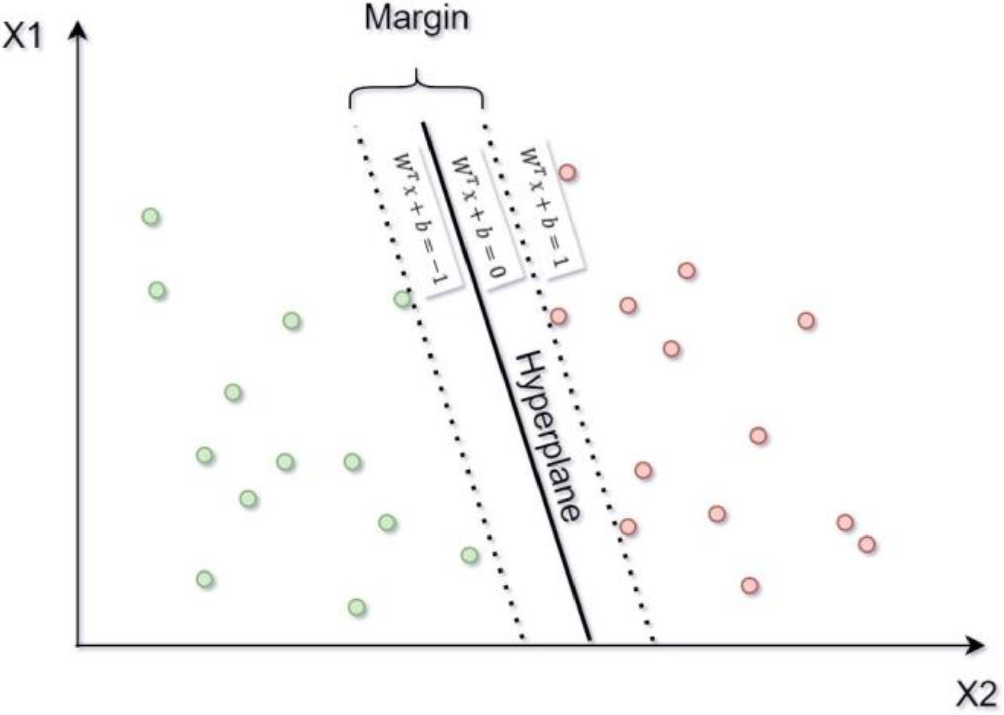
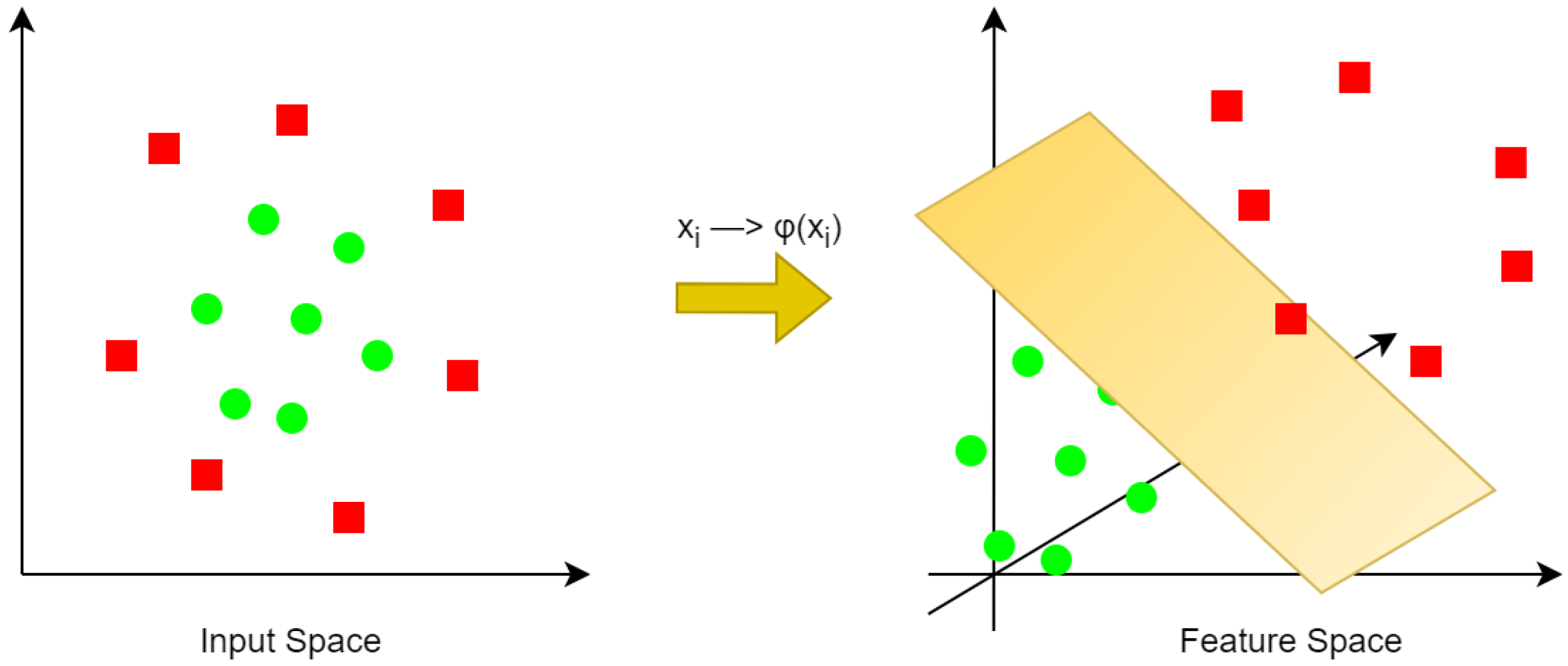
2.1. Support Vector Machine

Support Vector Machines (SVMs) are broadly used in engineering disciplines, as well as in mining and petroleum projects for reservoir characterization, permeability estimation, rock mass classification (RMR), and estimation of other important properties of rocks like uniaxial compressive strength (UCS) [33]. Support Vector Machines are supervised machine learning techniques used in regression, classification tasks, and the detection of outliers.

The main principle of SVM is to define a decision boundary between different classes or groups of variables that allows for the predictions of new labels according to the feature vector [34]. The decision boundaries, called hyperplanes, are located as far as possible between different classes and the closest samples or points of the classes to the hyperplane are called support vectors, as shown in Figure 4 [35]. In this case, a classifier is a linear straight line that can be defined as follows:

WTx + b = −1

(1)

where W is the weight vector, b is the bias term, and x is the input feature vector. The hyperplane must follow two main properties: (i) it is required to have the least error in the separation of the data, and (ii) the distance between the hyperplane and the closest data should be a maximum [33]. To address situations where data with similar features cannot be linearly separated, margins were employed to regulate the separability between classes. These margins were categorized as hard or soft, depending on whether the data points were allowed to enter the margin.

In the case of nonlinearity, the SVM used the kernel function, the objective of which was to map input data into a higher dimensional space called Hilbert or feature space for better generalization [36]. After mapping input data into a higher dimension, a support vector classifier or hyperplane was created to separate the data, as demonstrated in Figure 5 [33].

Support Vector Regression models are defined as mathematical models and several parameters need to be determined based on the data used. However, the specific number of parameters that highly impact the performance of the model, named as hyperparameters, cannot be learned straight from the data. Generally, hyperparameters are chosen by users based on their experience and trials. Depending on the used methods, many hyperparameters may need to be tuned and searching for the best combination is a key problem. SVM algorithms may use different types of kernels that attempt to transform the required data into the desired form. The most popular kernel functions are a linear kernel for simple classification problems; a polynomial kernel, which is a generalized representation of the linear kernel; a Gaussian Radial Basis Function (RBF) kernel that is mostly used for nonlinear data; and a sigmoid kernel used mainly for neural networks. In this experiment, the RBF was used due to its higher accuracy relative to the others, although it is more time-consuming. In the case of the RBF SVM, the important parameters C and Gamma were tuned to obtain the desired outcome.

The function of the C parameter is to control the error or margin of the hyperplane. When C is small, a decision boundary with a bigger margin is set, allowing more misclassifications. In contrast, a large C results in a smaller margin in the decision boundary by minimizing the number of misclassifications.

The Gamma parameter determines how the level of influence of each training example affects the result, with high values resulting in higher influence and low values leading to less influence. In order to visualize the influence of these parameters, Figure 6 illustrates the impact of the C and Gamma parameters on the decision function for a simple classification task on the Iris flower dataset [37]. As can be observed from Figure 6, the model was overly sensitive to the Gamma parameter. A large Gamma resulted in a small area of influence of support vectors that includes only itself, and the C parameter had no effect, consequently leading to overfitting. While Gamma was small, the large area of influence of the support vectors took into consideration the whole training sample, resulting in building constrained models that were not able to capture the complex relationship of the data [38]. Consequently, obtaining the optimal combination of the C and Gamma parameters is a computationally intensive task that requires multiple trials and a long time.

Optimal parameters were obtained via iterative computation using a grid search. The parameter range was continuous and unbound; thus, the range for the C and Gamma parameters were set manually between 0.1 and 20 and between 100 and 900, respectively. The determination of these ranges followed an iterative process involving experimentation with higher values of the C and Gamma parameters, leading to a reduction in the mean squared error observed between the test and train datasets. The data was split into train and test subsets (80% and 20%, respectively). The heatmap illustrated in Figure 7 shows the values of the mean squared error (MSE) between the test and training samples for a range of C and Gamma parameters. The heatmap highlights that the lowest MSE occurred when Gamma was around 300 and C was in the range of 9–10, as indicated by the yellow boxes. However, when utilizing these selected parameters, the predicted values exhibited a broader range of values that extend beyond the expected range (normalized values of 0 to 1). This can be explained by the fact that increasing the C parameter at a certain point of Gamma does not change the set of support vectors. As the MSE does not change significantly, decreasing the value of C was suggested since increasing the C value leads to a longer fitting time [38]. Moreover, when Gamma was too small, the model was constrained and did not capture the features or complexities of data. So, Gamma and C were decidedly selected as 1000 and 1, respectively, which resulted in a relatively good MSE.

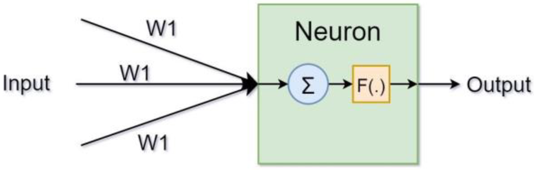
2.2. Multi-Layer Perceptron

Multi-Layer Perceptron is one of the most popular and versatile supervised neural network algorithms and is widely used for classification and regression tasks. A common MLP structure consists of at least three layers of nodes: input layers that obtain inputs or features, hidden layers, and output layers that generate the output results, as shown in Figure 8. The main principle of a neural network is as follows: after input variables are received, all calculations are carried out by hidden layers at each node. Each node includes a processing unit, called a neuron, that computes the sum of connection weights of inputs and passes through the nonlinear activation function to output nodes (Figure 9) [39,40,41].

A neural network consists of two phases: testing and training phases. In the training phase, the MLP is trained by supervised learning methods called back-propagation (BP) algorithms. Back-propagation is used to update the connection weights of the neural networks. In the testing phase, the results of the output are computed using a neural network and the error between the calculated and desired output is then used by the back- propagation (BP) algorithm to update the connection weights between nodes [39,42].

Multi-Layer Perceptron is a powerful feed-forward neural network that can predict unseen data (output) based on training data (input) by using a number of fully connected layers of nodes. The output (neuron) result is a weighted sum of inputs computed using an activation function. Tuning the hyperparameters of a neural network is more complex than for other machine learning algorithms. It can be divided into two parts. The first part is similar to the search grid as it was performed in the SVR method by trying different activation functions, optimizers, learning rates, and batch sizes. However, the second part, tuning the architecture of the neural network, is a challenging task as it is not straightforward. The depth of the algorithm is determined by the number of hidden layers, which is typically increased when dealing with complex data relationships. The number of neurons in each layer defines the width of the neural network and impacts the latent space, which is a representation of compressed data in which clusters of similar data are closer to each other in a space [43].

The selected hyperparameters presented in

Table 2. Hyperparameters of Multi-Layer Perceptron neural network.

Hidden layer size	200, 75, 50
Maximum number of iterations	40,000
Activation function	RELU
Solver function	LBFGS
Alpha	0.005
Learning rate	Constant

were determined based on empirical evaluation and consideration of their impact on the model’s performance. The hyperparameter alpha, which helps to control overfitting by penalizing the weights with larger values, was selected through trials on different values starting from 0.001 to 1, and the least MSE was observed with a 0.005 value for the alpha parameter. The rectified linear unit (ReLU) activation function, most commonly used due to its fast performance and simplicity on different tasks including prediction, was preferred. Moreover, this function discards all negative values by setting related activations as 0. In the case of the solver function, there are three options: optimizers such as “LBFGS” (limited-memory Broyden–Fletcher–Goldgarb–Shanno algorithm), “SGD” (stochastic gradient descent), and “ADAM” (stochastic gradient-based optimizer). It should be noted that “ADAM” works relatively well with big datasets; however, the number of training samples is around 5300, and the optimizer “LBFGS” performs better and faster in this case [38]. The learning rate was set to its default value, employing a “constant” learning rate schedule. Alternative options such as “inverse scaling” or “adaptive” were not chosen. In “inverse scaling,” the learning rate gradually decreases at each time step, while in “adaptive” scaling, the learning rate remains constant until the validation score fails to improve.

The architecture of MLP used for this specific task includes three layers. Determining the number of layers is essential, and at least 3 layers should be considered to learn a complex representation [44]. However, selecting the number of layers is a minor part of the larger problem as the user also needs to determine the number of neurons on each layer. This process was performed in the same way as the SVM procedure but with a different number of nodes in each layer, as shown in Figure 10, where the 3D heatmap shows squared mean errors computed between the test and predicted values. The least mean squared error was obtained when the architecture of the neural network had three layers with 200, 75, and 50 nodes.

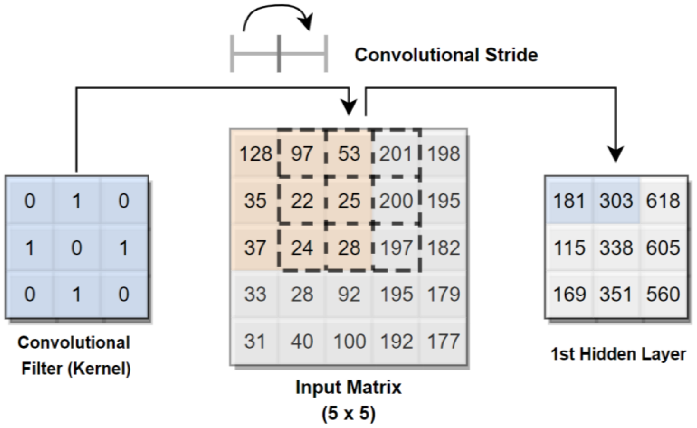
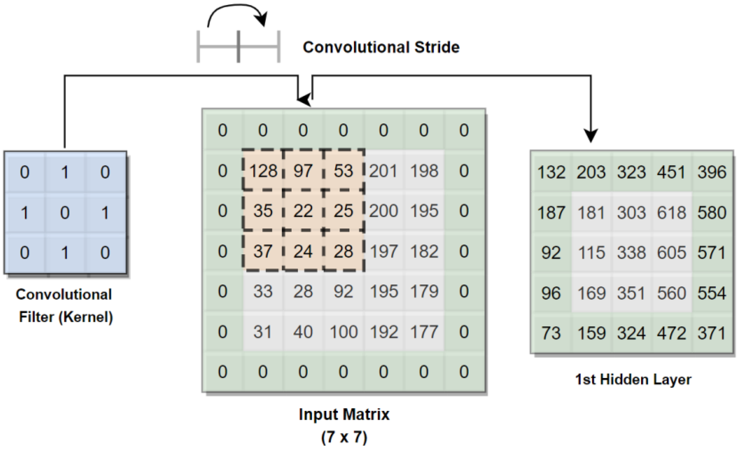
2.3. Convolutional Neural Network

Deep learning technologies are becoming a hot topic in medical imaging due to the vast range of applications, from the detection of diseases and cancer screening to specific treatment suggestions, by replacing time-consuming manual activities [45]. Some examples of the application of medical image processing include the detection of diabetic retinopathy [46,47,48,49], microscopical and histological elements [50,51], gastrointestinal diseases [52], quantification of calcium in cardiac images [53], tumour detection [54,55] and detection of Alzheimer’s and Parkinson’s disease [56,57,58].

In geoscience, deep learning technologies have started to be used in recent decades in weather forecasting, detection of effects of natural disasters, predicting soil moisture, classification of lithology, and resource estimation [59]. However, there is a lack of research on deep learning applications in resource estimation. Several studies were performed by combining deep learning techniques with multiple-point-statistics (MLS) simulation methods for modelling of spatial variables, as demonstrated by Avalos and Ortiz [60,61], where they used recursive Convolutional Neural Networks (CNN) in a MPS framework. Another similar study was completed by Tao and Pejman with a hybrid algorithm of CNN and MPS [62]. These pattern-based algorithms show improvements by using a CNN to fill the gap in missing regions. In addition, Generative Adversarial Neural Network (GAN) was used to mimic the global distribution in the case of categorical variables [63].

Among other deep learning techniques, Convolutional Neural Networks (CNN) are used increasingly in the geoscience field due to their outstanding performance in image processing; analyses such as segmentation, classification, and labelling; and most importantly, image reconstruction [64,65,66,67].

In this research, CNN is used for image reconstruction tasks, and it is important to investigate the structure of CNN. The structure of CNN consists of four parts: an input layer, a feature extraction zone, an inference zone, and an output layer, as shown in Figure 11. The input layer receives the image as a tensor, which is multi-dimensional data with different structures such as vectors, scalars, and matrices. In this case, the input image dimensions are nx, ny, nz, and nd, where x, y, and z are the spatial coordinates and d refers to the depth or number of channels in the image. For example, a colour image would have a depth of 3, due to its three channels: red, green, and blue.

The feature extraction zone is a combination of convolutional and pooling layers. In a convolutional layer, a set of convolutional filters or (learnable) kernels passes along an input matrix, as shown in Figure 12. In this example, the 3 × 3 convolutional filter has 9 convolutional operations that are involved in a 5 × 5 input matrix. It should be noted that the convolutional operation works separately on a different set of the 3 × 3 input matrix and the results include 9 different values in a 3 × 3 matrix on the 1st hidden layer, as shown in Figure 12 (right). The convolutional operation is a process of a kernel (filter) passing over an input matrix while executing the summation of an element-wise product of the corresponding convolutional filter (matrix 1) and input matrix (matrix 2). This kind of process can be applied again to the 1st hidden layer and again to the last hidden layer.

It should be noted that the CNN architecture processes an input image with a fixed size and the practitioner defines the size of the output volume by tuning the hyperparameters such as the filter size, convolutional stride, and spatial padding. The convolutional stride controls the number of nodes moved in each dimension of the next input slices. For instance, if the convolutional stride is (1,1), then the next convolutional operations starts one position or pixel to the right, as shown in Figure 12. After moving until the right edge of the matrix, convolutional operations start from left again but from second row. As noted in Figure 12, the convolved feature map is reduced in size on the 1st layer. Depending on the decision to keep the same size or to avoid a fast reduction in size, spatial padding is used. In the case of maintaining the same size between the hidden layers, spatial padding is used, where it pads the input with zeros around the border of the input to extend its size to 7 × 7, so that when the convolutional kernel is performed, the output matrix has the same size as shown in Figure 13.

Another important function of CNN is the pooling function, which is also called downsampling. A pooling operation partitions the input image into sub-regions and takes either the average or maximum values from sub-regions. There are several pooling functions, but the most widely used functions are average and max pooling [68].

Similar to the convolutional operation, the pooling operation divides the matrix in the same way and passes along an input matrix via convolutional strides. A max pooling example is given in Figure 14, where the pooling operation is performed using 2 × 2 slices and with 1 × 1 convolutional stride. As illustrated above, the pooling operation takes the maximum value out of four given values in a 2 × 2 slice. It is very common to insert pooling layers between convolutional layers in the CNN architecture to reduce the number of computations and thus memory footprint. Moreover, pooling layers helps to control overfitting of the model [69].

After extracting the features from an input image in the extraction zone, vector representation of the last hidden layer is used by the fully connected layers in the inference zone. So, the output of the last hidden layer is converted to a suitable format and fed to a multilayer feedforward network and backpropagation is applied repeatedly on each iteration by performing gradient descent. Gradient descent is a technique used for minimization of loss, where it adjusts the parameters for each iteration to find the best or optimal combination of weights and biases.

The idea of applying a CNN in resource estimation is based on the ability of the CNN to reconstruct the missing data. It should be noted that the problem of missing data can be divided into two classes: irregularly and regularly missing data. The former problem means that data are missing irregularly or randomly and the later means that data are missing periodically with the same missing gap between given samples. In this case, the regularly missing problem is considered to imitate the drillhole samples.

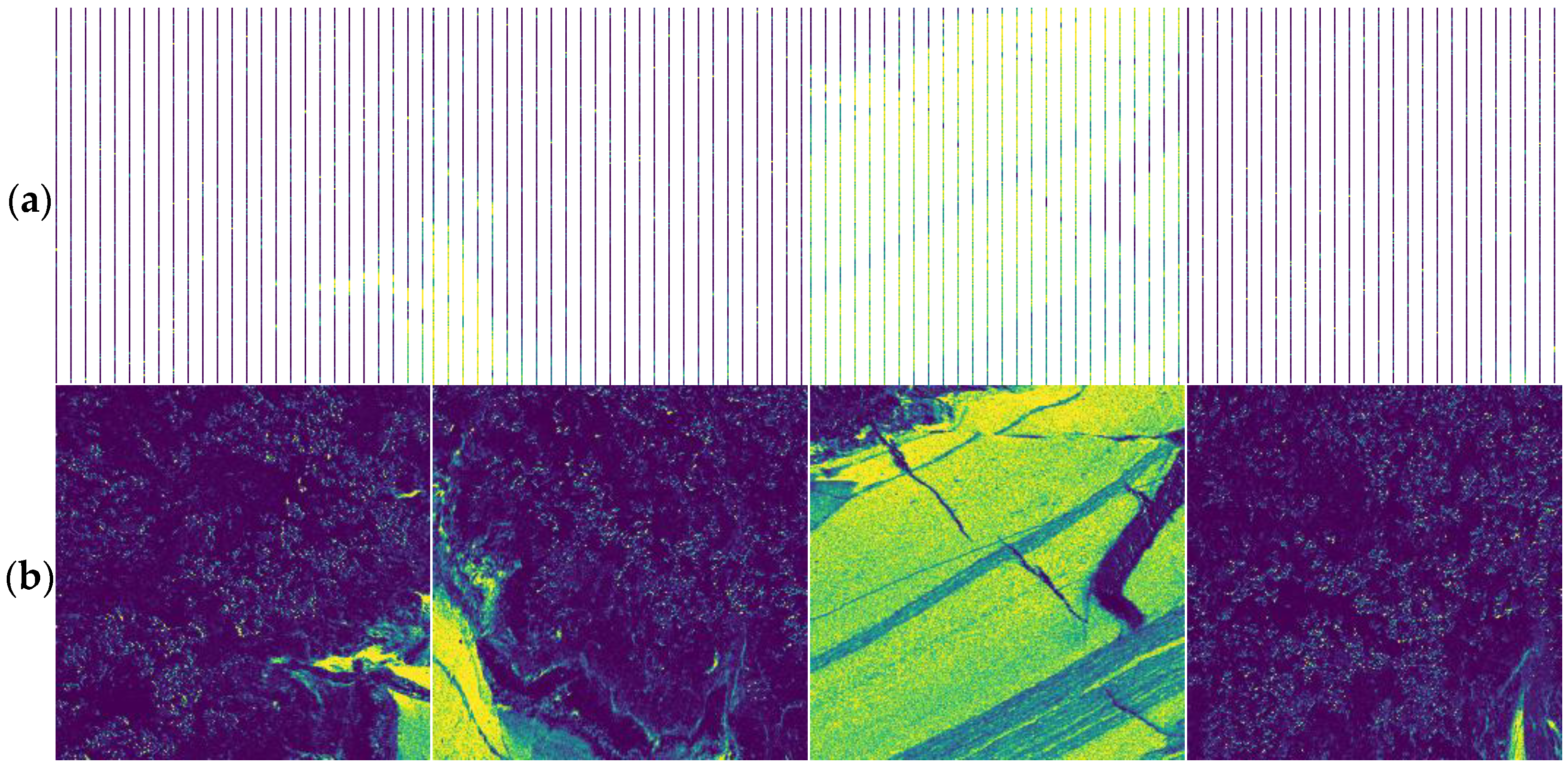
2.3.1. Training Images

Before starting to work with the Convolutional Neural Network, training images need to be prepared. There is widespread agreement that the successful application of a deep neural network requires a large number of training images [70]. In this research, a whole µXRF image of Zn-Pb-Ag ore from the George Fisher deposit showing the potassium concentration was used and split into hundreds of images, with a size of 256 × 256 pixels. To teach the CNN acceptable robustness and invariance, data augmentation was needed due to the small number of training images. The images were rotated 90, 180, and 270 degrees and the total number of training images after augmentation reached 1276. The input and output of the training images are shown in Figure 15, where 90% of the pixels were masked by removing each of the 9 columns of pixels iteratively. It should be mentioned that the training images were used to feed the CNN model, so the target images (target maps) to be predicted were removed from the training dataset. In other words, the CNN model did not receive target maps as input in advance.

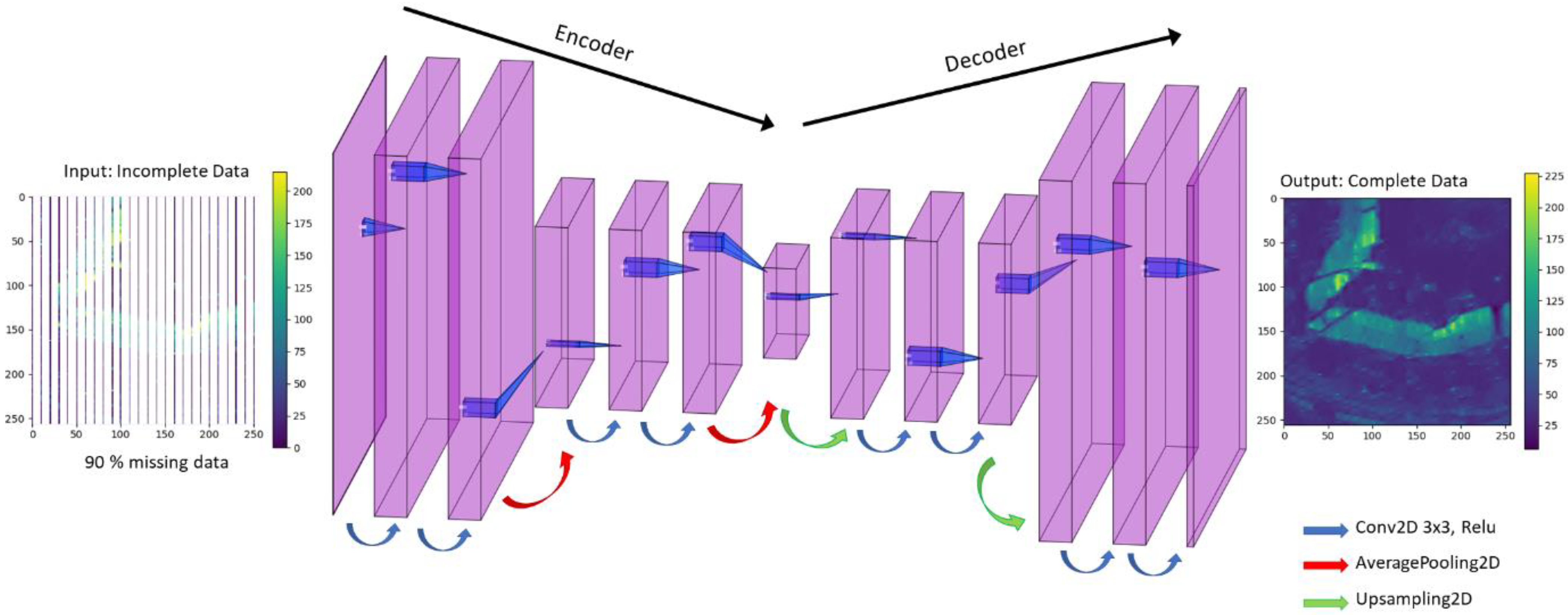
2.3.2. U-Net Architecture

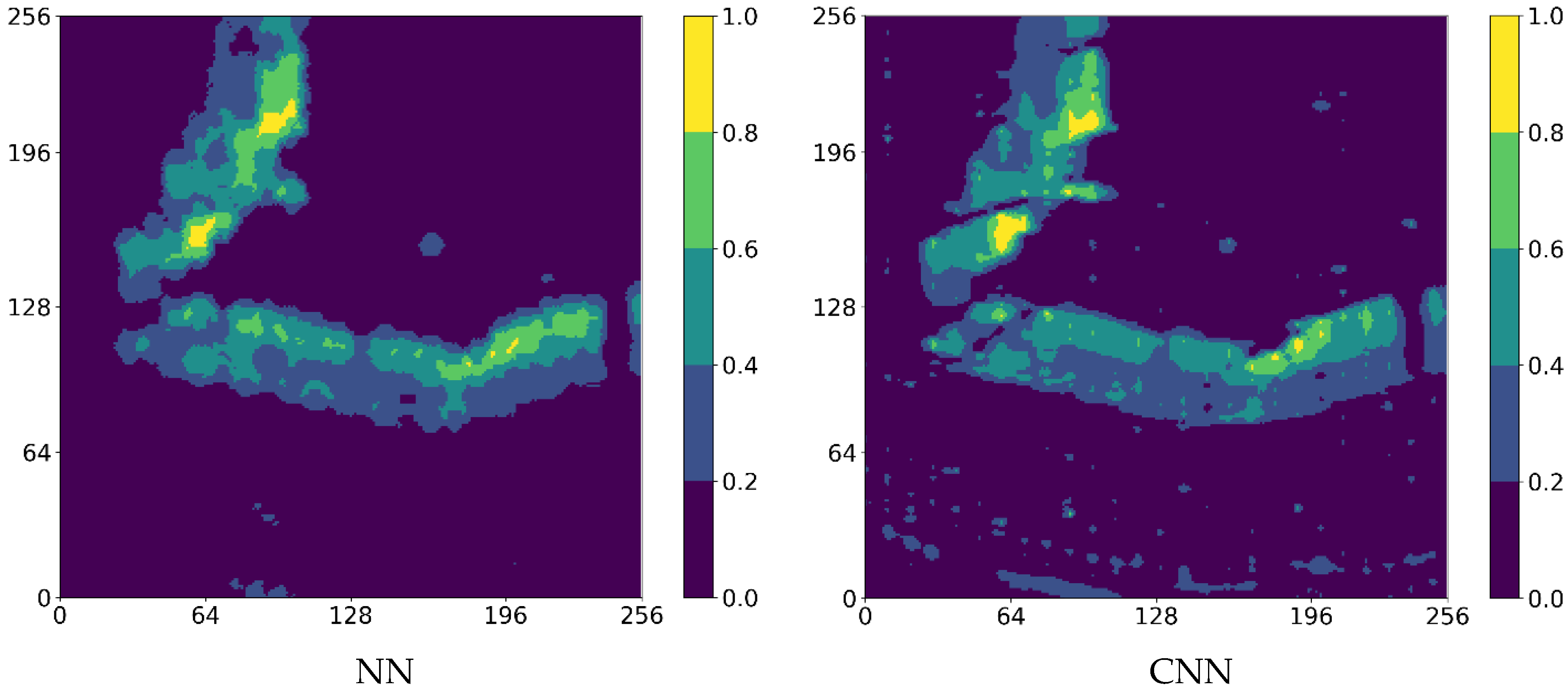
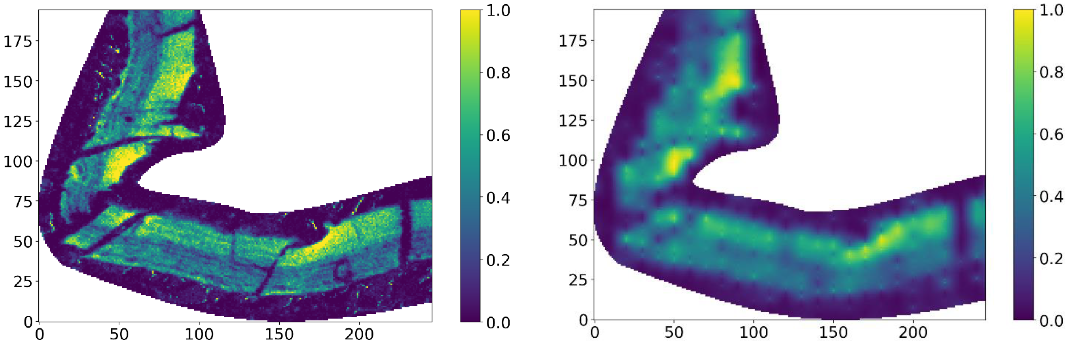
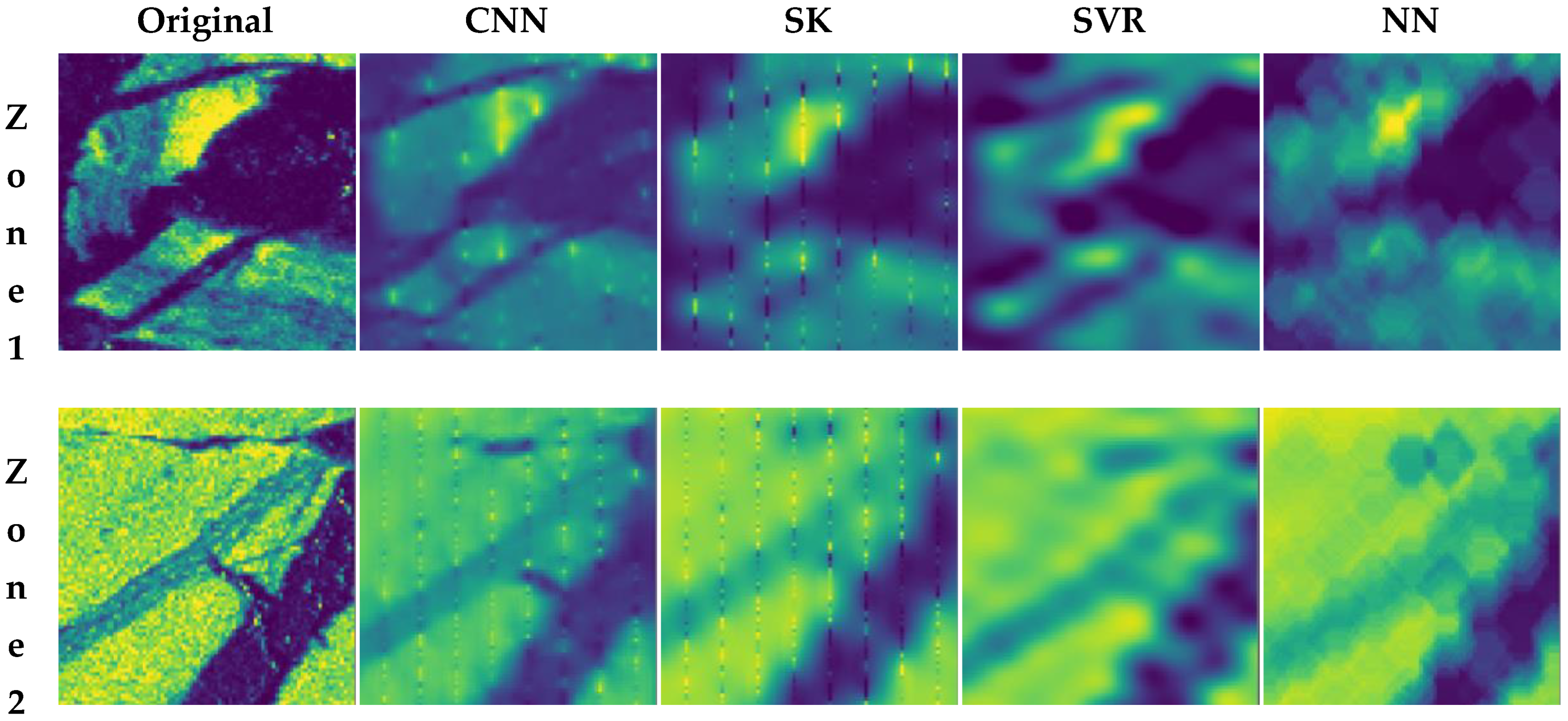
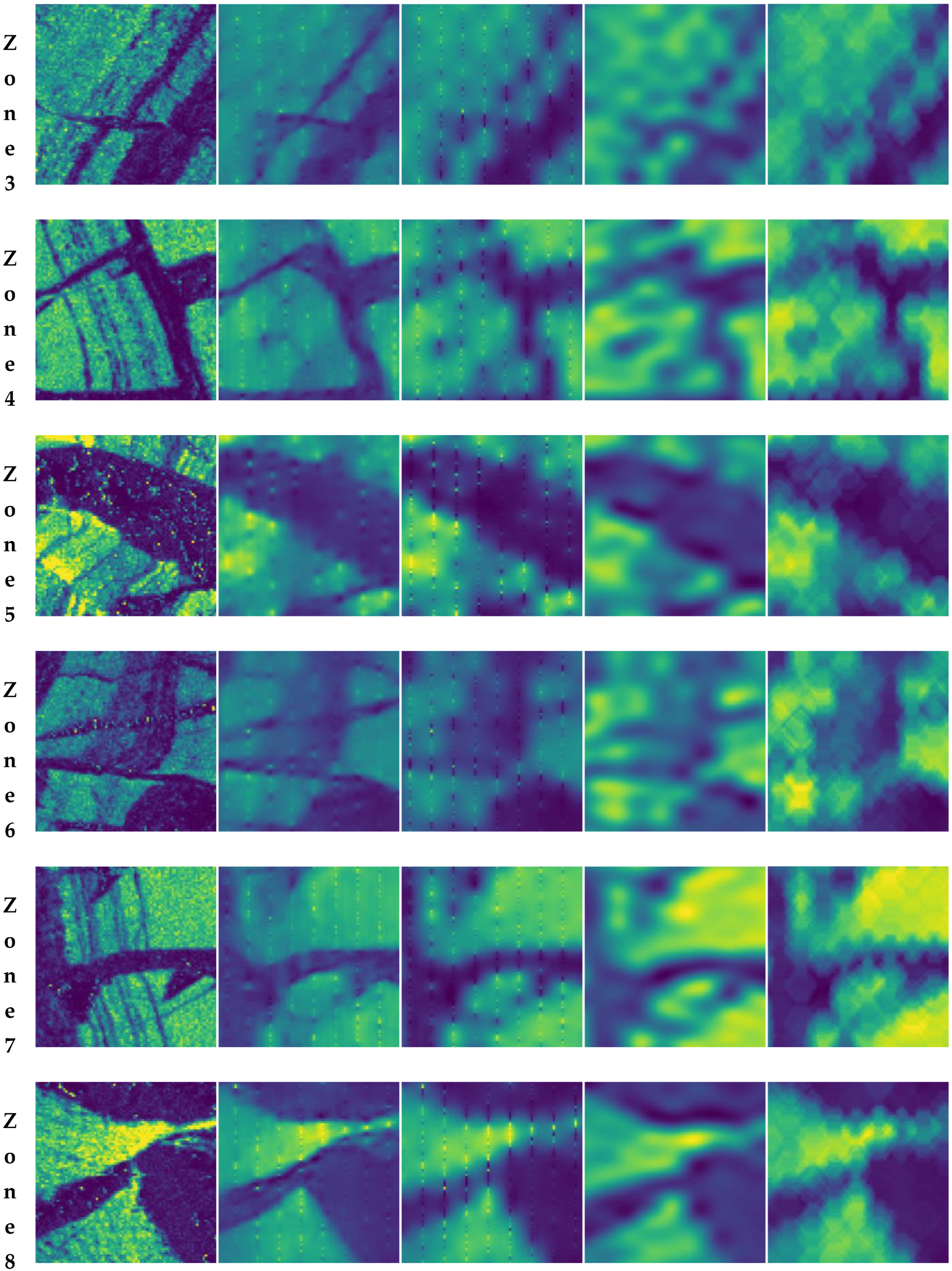
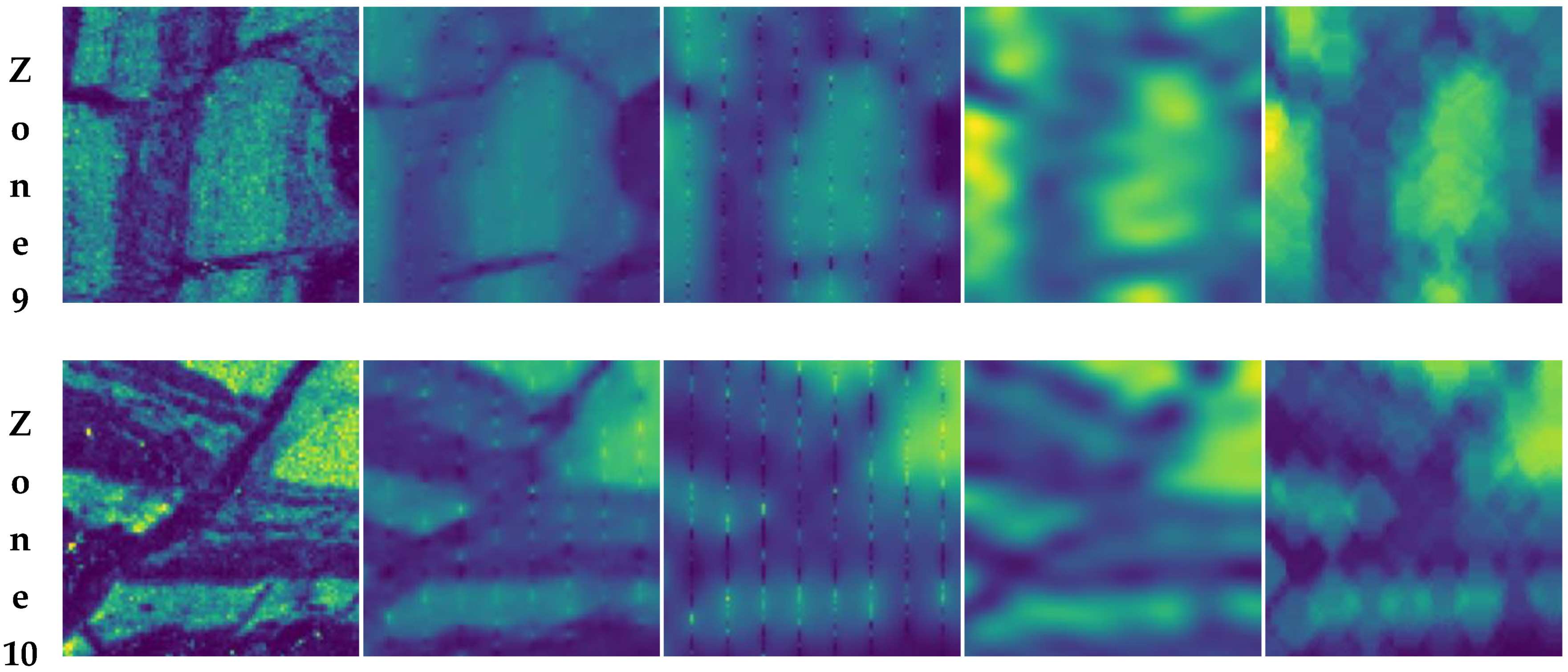
There is no rule about how many layers or what combination of convolutional and pooling layers are/is required to constitute the neural network; however, the generally accepted rule by many researchers is no less than 3 layers [71]. Specific to a given reconstruction task, a well-established group of neural networks, the U-net architecture, is used [67]. The scheme of U-net architecture is composed of contracting and expanding paths interpreted as encoders and decoders, as illustrated in Figure 16. As it can be seen from the illustration, in the encoding part, an image with missing data is taken as the input and convolutional layers continuously compute feature maps at different decreasing scales, resulting in multi-channel feature representation. In the decoder part, the layers synthesize or project discriminative features learned at a low resolution by the encoder onto a higher resolution (Figure 16). The loss function is based on the mean squared error (MSE), and a summary of the model can be seen in

Table 3. Model summary of the U-net structure.

Layer (Type)	Output Shape	Parameters
input_1 (InputLayer)	[(None, 256, 256, 1)]	0
conv2d (Conv2D)	(None, 256, 256, 32)	320
conv2d_1 (Conv2D)	(None, 256, 256, 32)	9248
average_pooling2d (AveragePooling)	(None, 128, 128, 32)	0
conv2d_2 (Conv2D)	(None, 128, 128, 32)	9248
conv2d_3 (Conv2D)	(None, 128, 128, 32)	9248
average_pooling2d_1 (AveragePooling)	(None, 64, 64, 32)	0
up_sampling2d (UpSampling2D)	(None, 128, 128, 32)	0
conv2d_4 (Conv2D)	(None, 128, 128, 32)	9248
conv2d_5 (Conv2D)	(None, 128, 128, 32)	9248
up_sampling2d_1 (UpSampling2)	(None, 256, 256, 32)	0
conv2d_6 (Conv2D)	(None, 256, 256, 32)	9248
conv2d_7 (Conv2D)	(None, 256, 256, 32)	9248
conv2d_8 (Conv2D)	(None, 256, 256, 1)	289
Total number of parameters		65,345
Number of trainable parameters		63,345

.

In a 2D CNN, the shape of the input image is typically represented as a 2-dimensional array, commonly referred to as a matrix or tensor. The dimensions of this matrix correspond to the height and width of the image, while the depth dimension represents the number of channels. The batch size is the number of training images fed to the model in one iteration. As the network does not know the batch size in advance, it is represented as None in the model summary (Table 3). The other three numbers represent the image dimensions with height, width, and depth. Depth of the image is the amount of colour information in each pixel, as mentioned before. In this case, the depth of the image is one, meaning only one channel (black and white). For instance, RGB images have 3 channels and greyscale images have 1 channel.

The total number of parameters learnt is 63,345. The input layer has a shape of [(None, 256, 256, 1)] and the parameter is 0, as the input layer has no learnable parameters. In the first convolutional layer, there are 32 filters, the kernel size through the whole network is 3 × 3, and the stride is 1. The number of parameters in the first convolutional layer is 320 from the equation below:

Number of parameters of 1st Conv layer = ((kernel size) × stride + 1) × (number of filters)

(2)

where 1 is added due to the bias term for each learned filter from the previous layer, so that

Number of parameters of 1st Conv Layer = ((3 × 3) × 1 + 1) × 32 = 320

(3)

The next convolutional layer has 9248 parameters as follows:

Number of parameters of 2nd Conv layer = ((kernel size) × stride × (number of filters from previous layer) + 1) × (number of filters)

(4)

Number of parameters of 2nd Conv Layer = ((3 × 3) × 1 × 32 + 1) × 32 = 9248

(5)

and so on. In the second part of the U-net structure, the decoder, upsampling takes place, which expands upon the feature dimensions to meet the size of the corresponding layers in the first part of the U-net structure, in the encoder. So, during upsampling, simple scaling of the image using Nearest Neighbourhood is performed with 2 × 2 scaling. In the last convolutional layer (conv2d_8), the number of parameters is equal to 289, as follows:

Number of parameters in the last Conv layer = ((kernel size) × stride × (number of filters from previous layer) + 1) × (number of filters)

(6)

Number of parameters in the last Conv Layer = ((3 × 3) × 1 × 32 + 1) × 1 = 289

(7)

where the number of filters is equal to 1, so the shape of the output is [(None, 256, 256, 1)] and the total number of all parameters is 63,345.

3. Results

The results shown are estimated or predicted maps of K (potassium) using Support Vector Regression (SVR) (Radial Basis Function), Multi-Layer Perceptron (MLP), Nearest Neighbourhood (NN), Convolutional Neural Network (CNN), and Simple Kriging (SK). It should be noted that the data were normalized (0,1) and fed into the ML techniques (SVR and MLP) as it is an important step in machine learning [68]. In the cases of Simple Kriging, Nearest Neighbourhood, and CNN, the estimated variables and images were normalized after the results were obtained in order to compare the techniques under the same conditions. The sizes of all predicted maps are 256 × 256 pixels.

Simple Kriging was computed using Stanford Geostatistical Modelling Software (SGeMS), which is an open-source computer package [72]. Nearest Neighbourhood was computed using the Python package for Nearest Neighbourhood by Scikit Learn [38].

In Simple Kriging, the grid size is the same as the number of pixels (X: 256, Y: 256, Z: 1) and the cell dimensions are 1 × 1 × 1. Spatial data are determined as isotropic since the nugget effect and the range are the same for all directions. Therefore, the omni-directional variogram was considered, as shown in Figure 17. The range of the search ellipsoid was taken as 50 × 50 × 50, which is a little bit less than the maximum range of variogram model [73].

In the case of the Nearest Neighbourhood, the unsampled location was estimated via local interpolation of the nearest neighbours in the training set. The optimal number of neighbours is between 12 and 15, as accuracies between the training and test results are higher in this range.

Figure 18 illustrates the predicted map obtained using all techniques mentioned above. As it can be inspected visually, the MLP technique produced the worst result in terms of following the geological features (shape and structure). In the cases of SVR, NN, and SK, the results show a smoothing effect that took place because of estimates based on the average weighted formula of Kriging [74]. The main reasons why MLP results in a poor reinstitution of the 2D maps can be due to a lack of consideration for the spatial structure [75] and reliance on manual feature engineering [76]. Moreover, fully connected architectures, like MLPs, have a greater risk of overfitting than the CNN architecture [77].

The produced images were displaced with intervals of 0.2 (0–0.2, 0.2–0.4, 0.6–0.8, and 0.8–1.0). This classification was performed to highlight the differences and to identify areas of high differences that are difficult to visualize in the case of regression results. Other intervals were also considered; however, more than five classes showed less difference with the regression map. Figure 19 illustrates the classified map constructed using all techniques, where CNN shows some fault structures represented in the original map of K.

In order to better identify the difference between the actual and predicted maps, an image differencing technique was computed by calculating the pairwise difference between pixels of predicted and actual classified maps. The least difference was shown in the results of Simple Kriging and Convolutional Neural Network, as shown in Figure 20. The results shown using MLP have about 20% difference in the region of waste, as expected. The rest of the results are relatively satisfactory and represent the orebody region with some noise (differences) on the map. CNN and SK show fewer relative differences that are noticeable in other methods.

The statistical comparison of results shown in

Table 4. Comparison table of different methods.

Methods	MSE	R2 Score
SVR	0.01600	0.63990
MLP	0.01518	0.65835
NN	0.01396	0.68570
CNN	0.01240	0.72084
SK	0.01118	0.74837

is based on the mean squared errors (MSE) and the regression score function (R² score). The regression score function is the proportion of variance in the dependent variable that is predictable from the independent variable. The best possible regression score is 1.0, and Table 4 provides the results of MSE and the regression score between the predicted and actual results for SVR, MLP, and NN. The lowest mean squared errors were obtained via CNN and SK with 0.01240 and 0.01118 values, respectively, as well as with higher regression scores, with 72.08% and 74.84%, respectively. The accuracies of the other results are lower. Despite the importance of statistical findings, they do not accurately reflect the authentic comparison due to the potential influence of a substantial portion of the map classified as waste, which has the potential to yield pseudo-positive or negative results. In this case, it is important to compare the results in ore zones, as in Figure 21, which is discussed in the next paragraph.

The results obtained in the zone of the orebody shows a slight change in the regression score and MSE results, as shown in

Table 5. Comparison table of different methods in ore region.

Methods	MSE	R2 Score
SVR	0.02531	0.66323
MLP	0.02735	0.63620
NN	0.02564	0.65886
CNN	0.01944	0.74141
SK	0.01901	0.74705

. As the waste zone was removed, MLP showed the lowest accuracy, as expected, followed by NN and SVR. SK and CNN showed similar accuracies, with 74.705% and 74.141%, respectively. In order to measure the detailed difference between the ground truth and predicted maps, the class of each cell (or pixel cell, 1 × 1 × 1) was subtracted from the corresponding class in the original map. The subtraction results were then summed in

Table 6. Comparison of difference between predicted and actual class maps.

SVM	MLP	NN	CNN	KRIG
2218.6	2253.0	2272.4	1884.4	1906

, where CNN showed the least difference, followed by Simple Kriging.

In order to properly validate all these techniques, 10 different maps were predicted in the same way in different regions of the whole image, as shown in Figure 22. For the rest of the results, the MLP technique was removed considering its inability to produce proper estimations, as discussed above.

By investigating all results using four different techniques, we observed that, statistically, Simple Kriging and Convolutional Neural Network performed better by showing higher accuracy and lower mean squared errors. The Nearest Neighbourhood and Support Vector Regression techniques returned lower accuracies and higher errors, as shown in Figure 23, which is a summary of all the results in the different regions. Regions 4 and 9 have additional results where the waste zone was removed (named as 4 cut and 9 cut, respectively). This was carried out to see how the performance change when a big portion of waste zone is removed.

Further investigation of the estimated images shows that one of the main limitations of CNN that is noticed within almost all regions is that the frequency distribution of predicted values shown in the histogram results are not well reproduced. In this case, the CNN results show frequency distributions with less range, indicating that distribution is not reproduced well as the maximum and minimum values are squeezed. Figure 24 shows the histograms with 10 intervals of original data, training data, and produced results from SVM, NN, CNN, and SK in zone 1. The original data have a count of about 45,000 and 5000 samples within the first (0–0.1) and second (0.1–0.2) bins, respectively; however, CNN has about 30,000 and 16,000 samples within the respective bins. This kind of behaviour can be noticed in almost all examples. Consequently, this issue might lead to less accuracy than expected.

4. Discussion

A comparison of geologic features such as discontinuities, faults, and domain boundaries produced via Convolutional Neural Network (CNN), Simple Kriging (SK), Support Vector Regression (SVR), and Nearest Neighbourhood (NN) in different zones is shown in Figure 25, which displays magnified sections of the predicted maps for all ten regions. In every zone, the CNN technique leads by constructing a better representation of geology by effectively defining domain borders and constructing discontinuities, specifically faults within veins. Fed by the training images, the CNN is capable of capturing important features of each training image based on thousands of calculations and analyses and has a good ability to define borders of domains and to construct discontinuities. From all the results from Figure 25, it can be seen that the CNN demonstrates the capability to effectively reproduce the intrinsic characteristics of given data and shows potential superiority over other techniques.

The main advantage of a CNN is its capability to learn local features from the input data. A CNN is a powerful tool in image processing tasks and can capture relevant features such as edges, corners, or textures of the image. In this case, during the training of the model, the convolutional filters (learnable kernels) successfully captured patterns of the data such as geological shapes including veins and faults, as it can be seen in Figure 25. Based on the quantitative comparison of the performance from Table 6, the CNN shows the least difference compared with the ground truth, followed by SK.

It is important to note that CNNs benefit from utilizing available training data, which may introduce bias when comparing them with interpolation techniques and ML approaches that solely rely on sample data. However, the focus of this research is to emphasize the potential of CNN application, particularly in ongoing projects where the training data are accessible. Consequently, the dependence on high-quality training data is the main challenge in the effective implementation of CNNs. Moreover, it is necessary to further investigate the impact of different CNN architectures on their prediction ability.

Another significant challenge is the application of CNN in 3D datasets since the ultimate objective of the research is to enable prediction in the 3D spatial data. For this purpose, the research project is currently working on designing a 3D CNN architecture that will allow 3D datasets to be used. However, the construction of an optimal 3D CNN architecture that will result in the best performance is a very tedious and challenging task due to thousands of different parameters that can be changed in the design of the architecture. Consequently, another aim of the research is to provide a guideline to implement the CNN approach in 3D spatial predictions.

It should be noted that the required computational time of each technique varies based on their implementation steps. While the prediction of the trained DL technique is instant, the training phase of the DL technique is the most computationally intensive and the time required depends on user-defined parameters such as early stopping criteria. Moreover, the initial weights of the model can impact training time, as they can be either close to or far from optimal parameters. On the other hand, ML and interpolation techniques using sample data have shorter computational time.

Once the issue with the frequency distribution highlighted above is solved, it is likely that the CNN will show better results than other techniques, not only by following the intrinsic characteristics of the geology but also statistically.

Considering all the results and observations, future work should focus on solving the distribution problem of the CNN results. The main steps that could possibly solve this limitation are as follows:

-

Investigation of the CNN layers and their combination to change the output results to follow the statistics of the input;

-

Optimization of the CNN structure and hyperparameters;

-

Use of more training images to be fed into the CNN model. As suggested by the literature review, more training images lead to better results. The training images can be expanded more by editing, flipping, and adjusting the level of saturation and brightness;

-

Post-processing steps of the result to make the distribution of predicted data follow the distribution of input data;

-

Application of other validation techniques such as statistical significance tests.

Further future work includes other project steps that aim to integrate 3D CNN into resource estimation by creating guidelines or instructions that will aid in the construction of 3D CNN structure based on dataset characteristics. Moreover, using additional information such as structural data, lithology, and mineralization is considered in the project scope.

5. Conclusions

This study utilizes a deep learning framework based on an encoder–decoder U-net CNN to predict unknown sample values of potassium on 2D maps. The evaluation of results from different methods supports the effectiveness of CNN in prediction tasks by leveraging intrinsic data characteristics such as faults and shapes. Convolutional Neural Networks (CNNs) offer benefits such as the ability to define borders and to capture features such as discontinuities, specifically faults within veins. However, they also have weaknesses including dependence on training data, complexity in architecture design and parameter tuning, and limited interpretability. Further research is required to explore the impact of different CNN architectures on prediction ability and to address the distribution problem in CNN results. It should be emphasized that results may differ when working with 3D data. Future research should address these considerations to enhance the understanding and applicability of DL techniques.

References

1. Dimitrakopoulos, R. Stochastic mine planning—Methods, examples and value in an uncertain world. In Advances in Applied Strategic Mine Planning; Springer: Cham, Switzerland, 2018; pp. 101–115. [Google Scholar]
2. Sterk, R.; de Jong, K.; Partington, G.; Kerkvliet, S.; van de Ven, M. Domaining in Mineral Resource Estimation: A Stock-Take of 2019 Common Practice. In Proceedings of the 11th International Mining Geology Conference, Perth, Australia, 5–26 November 2019. [Google Scholar]
3. McManus, S.; Rahman, A.; Coombes, J.; Horta, A. Uncertainty assessment of spatial domain models in early stage mining projects—A review. Ore Geol. Rev. 2021, 133, 104098. [Google Scholar] [CrossRef]
4. Rossi, M.E.; Deutsch, C.V. Mineral Resource Estimation; Springer Science & Business Media: Berlin, Germany, 2013. [Google Scholar]
5. Goovaerts, P. Geostatistics for Natural Resources Evaluation; Oxford University Press on Demand: Oxford, UK, 1997. [Google Scholar]
6. Madani, N.; Maleki, M.; Soltani-Mohammadi, S. Geostatistical modeling of heterogeneous geo-clusters in a copper deposit integrated with multinomial logistic regression: An exercise on resource estimation. Ore Geol. Rev. 2022, 150, 105132. [Google Scholar] [CrossRef]
7. Madenova, Y.; Madani, N. Application of Gaussian mixture model and geostatistical co-simulation for resource modeling of geometallurgical variables. Nat. Resour. Res. 2021, 30, 1199–1228. [Google Scholar] [CrossRef]
8. Battalgazy, N.; Madani, N. Stochastic modeling of chemical compounds in a limestone deposit by unlocking the complexity in bivariate relationships. Minerals 2019, 9, 683. [Google Scholar] [CrossRef] [Green Version]
9. Abildin, Y.; Madani, N.; Topal, E. A hybrid approach for joint simulation of geometallurgical variables with inequality constraint. Minerals 2019, 9, 24. [Google Scholar] [CrossRef] [Green Version]
10. Emery, X.; Lantuéjoul, C. Tbsim: A computer program for conditional simulation of three-dimensional gaussian random fields via the turning bands method. Comput. Geosci. 2006, 32, 1615–1628. [Google Scholar] [CrossRef]
11. Battalgazy, N.; Madani, N. Categorization of mineral resources based on different geostatistical simulation algorithms: A case study from an iron ore deposit. Nat. Resour. Res. 2019, 28, 1329–1351. [Google Scholar] [CrossRef]
12. Armstrong, M.; Galli, A.; Beucher, H.; Loc’h, G.; Renard, D.; Doligez, B.; Eschard, R.; Geffroy, F. Plurigaussian Simulations in Geosciences; Springer Science & Business Media: Berlin, Germany, 2011. [Google Scholar]
13. Prior, T.; Giurco, D.; Mudd, G.; Mason, L.; Behrisch, J. Resource depletion, peak minerals and the implications for sustainable resource management. Glob. Environ. Chang. 2012, 22, 577–587. [Google Scholar] [CrossRef]
14. Valenta, R.; Kemp, D.; Owen, J.; Corder, G.; Lèbre, É. Re-thinking complex orebodies: Consequences for the future world supply of copper. J. Clean. Prod. 2019, 220, 816–826. [Google Scholar] [CrossRef]
15. Delgado, A.V. Mineral resource depletion assessment. In Eco-Efficient Construction and Building Materials; Elsevier: Amsterdam, The Netherlands, 2014; pp. 13–37. [Google Scholar]
16. West, J. Decreasing Metal Ore Grades: Are They Really Being Driven by the Depletion of High-Grade Deposits? J. Ind. Ecol. 2011, 15, 165–168. [Google Scholar] [CrossRef]
17. Caté, A.; Perozzi, L.; Gloaguen, E.; Blouin, M. Machine learning as a tool for geologists. Lead. Edge 2017, 36, 215–219. [Google Scholar] [CrossRef]
18. Hill, E.J.; Oliver, N.H.; Fisher, L.; Cleverley, J.S.; Nugus, M.J. Using geochemical proxies to model nuggety gold deposits: An example from Sunrise Dam, Western Australia. J. Geochem. Explor. 2014, 145, 12–24. [Google Scholar] [CrossRef]
19. Jalloh, A.B.; Kyuro, S.; Jalloh, Y.; Barrie, A.K. Integrating artificial neural networks and geostatistics for optimum 3D geological block modeling in mineral reserve estimation: A case study. Int. J. Min. Sci. Technol. 2016, 26, 581–585. [Google Scholar] [CrossRef]
20. Dutta, S.; Bandopadhyay, S.; Ganguli, R.; Misra, D. Machine learning algorithms and their application to ore reserve estimation of sparse and imprecise data. J. Intell. Learn. Syst. Appl. 2010, 2, 86. [Google Scholar] [CrossRef] [Green Version]
21. Tahmasebi, P.; Hezarkhani, A. A hybrid neural networks-fuzzy logic-genetic algorithm for grade estimation. Comput. Geosci. 2012, 42, 18–27. [Google Scholar] [CrossRef] [PubMed] [Green Version]
22. Chatterjee, S.; Bandopadhyay, S.; Machuca, D. Ore grade prediction using a genetic algorithm and clustering based ensemble neural network model. Math. Geosci. 2010, 42, 309–326. [Google Scholar] [CrossRef]
23. Wu, X.; Zhou, Y. Reserve estimation using neural network techniques. Comput. Geosci. 1993, 19, 567–575. [Google Scholar] [CrossRef]
24. Guo, W.W. A novel application of neural networks for instant iron-ore grade estimation. Expert Syst. 2010, 37, 8729–8735. [Google Scholar] [CrossRef]
25. Nezamolhosseini, S.A.; Mojtahedzadeh, S.H.; Gholamnejad, J. The application of artificial neural networks to ore reserve estimation at choghart iron ore deposit. J. Anal. Numer. Methods Min. Eng. 2017, 6, 73–83. [Google Scholar]
26. Afeni, T.B.; Lawal, A.I.; Adeyemi, R.A. Re-examination of Itakpe iron ore deposit for reserve estimation using geostatistics and artificial neural network techniques. Arab. J. Geosci. 2020, 13, 657. [Google Scholar] [CrossRef]
27. Li, X.-L.; Li, L.-H.; Zhang, B.-L.; Guo, Q.-J. Hybrid self-adaptive learning based particle swarm optimization and support vector regression model for grade estimation. Neurocomputing 2013, 118, 179–190. [Google Scholar] [CrossRef]
28. Mostafaei, K.; Jodeiri, B. A new gold grade estimation approach by using support vector machine (SVM) and back propagation neural network (BPNN)-A Case study: Dalli deposit, Iran. arXiv 2022, arXiv:2008568. [Google Scholar]
29. Abbaszadeh, M. Grade Estimation in Esfordi Phosphate Deposit Using Support Vector Regression Method. J. Miner. Resour. Eng. 2019, 4, 1–16. [Google Scholar]
30. Chatterjee, S.; Bandopadhyay, S. Goodnews Bay Platinum resource estimation using least squares support vector regression with selection of input space dimension and hyperparameters. Nat. Resour. Res. 2011, 20, 117–129. [Google Scholar] [CrossRef]
31. Zaki, M.; Chen, S.; Zhang, J.; Feng, F.; Khoreshok, A.A.; Mahdy, M.A.; Salim, K.M. A Novel Approach for Resource Estimation of Highly Skewed Gold Using Machine Learning Algorithms. Minerals 2022, 12, 900. [Google Scholar] [CrossRef]
32. Barker, R.D.; Barker, S.L.; Wilson, S.A.; Stock, E.D. Quantitative Mineral Mapping of Drill Core Surfaces I: A Method for µ XRF Mineral Calculation and Mapping of Hydrothermally Altered, Fine-Grained Sedimentary Rocks from a Carlin-Type Gold Deposit. Econ. Geol. 2021, 116, 803–819. [Google Scholar] [CrossRef]
33. Gholami, R.; Fakhari, N. Support vector machine: Principles, parameters, and applications. In Handbook of Neural Computation; Elsevier: Amsterdam, The Netherlands, 2017; pp. 515–535. [Google Scholar]
34. Noble, W.S. What is a support vector machine? Nat. Biotechnol. 2006, 24, 1565–1567. [Google Scholar] [CrossRef]
35. Huang, S.; Cai, N.; Pacheco, P.P.; Narrandes, S.; Wang, Y.; Xu, W. Applications of support vector machine (SVM) learning in cancer genomics. Cancer Genom. Proteom. 2018, 15, 41–51. [Google Scholar]
36. Mercer, J. Xvi. functions of positive and negative type, and their connection the theory of integral equations. Philos. Trans. R. Soc. Lond. Ser. A Contain. Pap. A Math. Phys. Character 1909, 209, 415–446. [Google Scholar]
37. Fisher, R.A. The use of multiple measurements in taxonomic problems. Ann. Eugen. 1936, 7, 179–188. [Google Scholar] [CrossRef]
38. Pedregosa, F.; Varoquaux, G.; Gramfort, A.; Michel, V.; Thirion, B.; Grisel, O.; Blondel, M.; Prettenhofer, P.; Weiss, R.; Dubourg, V. Scikit-learn: Machine learning in Python. J. Mach. Learn. Res. 2011, 12, 2825–2830. [Google Scholar]
39. Hasan, T.T.; Jasim, M.H.; Hashim, I.A. Heart disease diagnosis system based on multi-layer perceptron neural network and support vector machine. Int. J. Curr. Eng. Technol. 2017, 77, 2277–4106. [Google Scholar]
40. Wan, S.; Liang, Y.; Zhang, Y.; Guizani, M. Deep multi-layer perceptron classifier for behavior analysis to estimate Parkinson’s disease severity using smartphones. IEEE Access 2018, 6, 36825–36833. [Google Scholar] [CrossRef]
41. Yan, C.; Yi, W.; Xiong, J.; Ma, J. Preparation and visible light photocatalytic activity of Bi2O3/Bi2WO6 heterojunction photocatalysts. In Proceedings of the IOP Conference Series: Earth and Environmental Science, Beijing, China, 28–31 December 2017; p. 012086. [Google Scholar]
42. Sharma, P.; Singh, D.; Bandil, M.K.; Mishra, N. Decision support system for malaria and dengue disease diagnosis (DSSMD). Int. J. Inf. Comput. Technol. 2013, 3, 633–640. [Google Scholar]
43. Weissbart, L. Performance analysis of multilayer perceptron in profiling side-channel analysis. In Proceedings of the International Conference on Applied Cryptography and Network Security, Rome, Italy, 19–22 October 2020; pp. 198–216. [Google Scholar]
44. Heaton, J. Artificial Intelligence for Humans, Volume 3: Deep Learning and Neural Networks; Heaton Research, Inc.: St. Louis, MO, USA, 2015. [Google Scholar]
45. Suzuki, K. Overview of deep learning in medical imaging. Radiol. Phys. Technol. 2017, 10, 257–273. [Google Scholar] [CrossRef]
46. Alban, M.; Gilligan, T. Automated Detection of Diabetic Retinopathy Using Fluorescein Angiography Photographs, in Report of Standford Education. 2016. Available online: http://cs231n.stanford.edu/reports/2016/pdfs/309_Report.pdf (accessed on 22 June 2023).
47. Gulshan, V.; Peng, L.; Coram, M.; Stumpe, M.C.; Wu, D.; Narayanaswamy, A.; Venugopalan, S.; Widner, K.; Madams, T.; Cuadros, J. Development and validation of a deep learning algorithm for detection of diabetic retinopathy in retinal fundus photographs. JAMA 2016, 316, 2402–2410. [Google Scholar] [CrossRef]
48. Pratt, H.; Coenen, F.; Broadbent, D.M.; Harding, S.P.; Zheng, Y. Convolutional neural networks for diabetic retinopathy. Procedia Comput. Sci. 2016, 90, 200–205. [Google Scholar] [CrossRef] [Green Version]
49. San, G.L.Y.; Lee, M.L.; Hsu, W. Constrained-MSER detection of retinal pathology. In Proceedings of the 21st International Conference on Pattern Recognition (ICPR2012), Tsukuba, Japan, 11–15 November 2012; pp. 2059–2062. [Google Scholar]
50. Bayramoglu, N.; Heikkilä, J. Transfer learning for cell nuclei classification in histopathology images. In Proceedings of the European Conference on Computer Vision, Amsterdam, The Netherlands, 8–10 and 15–16 October 2016; pp. 532–539. [Google Scholar]
51. Razzak, M.I.; Alhaqbani, B. Automatic detection of malarial parasite using microscopic blood images. J. Med. Imaging Health Inform. 2015, 5, 591–598. [Google Scholar] [CrossRef]
52. Jia, X.; Meng, M.Q.-H. A deep convolutional neural network for bleeding detection in wireless capsule endoscopy images. In Proceedings of the 2016 38th Annual International Conference of the IEEE Engineering in Medicine and Biology Society (EMBC), Orlando, FL, USA, 16–20 August 2016; pp. 639–642. [Google Scholar]
53. Wolterink, J.M.; Leiner, T.; Viergever, M.A.; Išgum, I. Automatic coronary calcium scoring in cardiac CT angiography using convolutional neural networks. In Proceedings of the International Conference on Medical Image Computing and Computer-Assisted Intervention, Munich, Germany, 5–9 October 2015; pp. 589–596. [Google Scholar]
54. Kooi, T.; van Ginneken, B.; Karssemeijer, N.; den Heeten, A. Discriminating solitary cysts from soft tissue lesions in mammography using a pretrained deep convolutional neural network. Med. Phys. 2017, 44, 1017–1027. [Google Scholar] [CrossRef] [Green Version]
55. Wang, Z.; Yu, G.; Kang, Y.; Zhao, Y.; Qu, Q. Breast tumor detection in digital mammography based on extreme learning machine. Neurocomputing 2014, 128, 175–184. [Google Scholar] [CrossRef]
56. Huynh, B.; Drukker, K.; Giger, M. MO-DE-207B-06: Computer-aided diagnosis of breast ultrasound images using transfer learning from deep convolutional neural networks. Med. Phys. 2016, 43, 3705. [Google Scholar] [CrossRef]
57. Sarraf, S.; Tofighi, G.; Anderson, J. Deepad: Alzheimer’s disease classification via deep convolutional neural networks using mri and fmri. bioRxiv 2016. bioRxiv: 070441. [Google Scholar]
58. Shin, H.-C.; Roth, H.R.; Gao, M.; Lu, L.; Xu, Z.; Nogues, I.; Yao, J.; Mollura, D.; Summers, R.M. Deep convolutional neural networks for computer-aided detection: CNN architectures, dataset characteristics and transfer learning. IEEE Trans. Med. Imaging 2016, 35, 1285–1298. [Google Scholar] [CrossRef] [Green Version]
59. Zuo, R.; Xiong, Y.; Wang, J.; Carranza, E.J.M. Deep learning and its application in geochemical mapping. Earth Sci. Rev. 2019, 192, 1–14. [Google Scholar] [CrossRef]
60. Avalos, S.; Ortiz, J.M. Geological modeling using a recursive convolutional neural networks approach. arXiv 2019, arXiv:1904.12190. [Google Scholar]
61. Avalos, S.; Ortiz, J.M. Recursive convolutional neural networks in a multiple-point statistics framework. Comput. Geosci. 2020, 141, 104522. [Google Scholar] [CrossRef]
62. Bai, T.; Tahmasebi, P. Hybrid geological modeling: Combining machine learning and multiple-point statistics. Comput. Geosci. 2020, 142, 104519. [Google Scholar] [CrossRef]
63. Chan, S.; Elsheikh, A.H. Parametrization of stochastic inputs using generative adversarial networks with application in geology. Front. Water 2020, 2, 5. [Google Scholar] [CrossRef]
64. Eilertsen, G.; Kronander, J.; Denes, G.; Mantiuk, R.K.; Unger, J. HDR image reconstruction from a single exposure using deep CNNs. ACM Trans. Graph. (TOG) 2017, 36, 1–15. [Google Scholar] [CrossRef] [Green Version]
65. Farabet, C.; Couprie, C.; Najman, L.; LeCun, Y. Learning hierarchical features for scene labeling. IEEE Trans. Pattern Anal. Mach. Intell. 2012, 35, 1915–1929. [Google Scholar] [CrossRef] [PubMed] [Green Version]
66. He, K.; Zhang, X.; Ren, S.; Sun, J. Deep residual learning for image recognition. In Proceedings of the IEEE Conference on Computer Vision and Pattern Recognition, Las Vegas, NV, USA, 27–30 June 2016; pp. 770–778. [Google Scholar]
67. Shelhamer, E.; Long, J.; Darrell, T. Fully convolutional networks for semantic segmentation. IEEE Trans. Pattern Anal. Mach. Intell. 2016, 39, 640–651. [Google Scholar] [CrossRef] [PubMed]
68. Géron, A. Hands-On Machine Learning with Scikit-Learn, Keras, and TensorFlow: Concepts, Tools, and Techniques to Build Intelligent Systems; O’Reilly Media, Inc.: Sebastopol, CA, USA, 2019. [Google Scholar]
69. Goodfellow, I.; Bengio, Y.; Courville, A. Deep Learning; MIT Press: Cambridge, MA, USA, 2016. [Google Scholar]
70. Ronneberger, O.; Fischer, P.; Brox, T. U-net: Convolutional networks for biomedical image segmentation. In Proceedings of the International Conference on Medical Image Computing and Computer-Assisted Intervention, Munich, Germany, 5–9 October 2015; pp. 234–241. [Google Scholar]
71. Chai, X.; Gu, H.; Li, F.; Duan, H.; Hu, X.; Lin, K. Deep learning for irregularly and regularly missing data reconstruction. Sci. Rep. 2020, 10, 3302. [Google Scholar] [CrossRef] [PubMed] [Green Version]
72. Remy, N.; Boucher, A.; Wu, J. Applied Geostatistics with SGeMS: A User’s Guide; Cambridge University Press: Cambridge, UK, 2009. [Google Scholar]
73. Asghari, O.; Safikhani, M.; Talesh Hosseini, S. Determining the optimum search range for 2D and 3D mapping based on kriging through quantitative analysis. Boll. Geofis. Teor. Appl. 2020, 61, 177–198. [Google Scholar]
74. Yamamoto, J.K. Correcting the smoothing effect of ordinary kriging estimates. Math. Geol. 2005, 37, 69–94. [Google Scholar] [CrossRef]
75. LeCun, Y.; Bottou, L.; Bengio, Y.; Haffner, P. Gradient-based learning applied to document recognition. Proc. IEEE 1998, 86, 2278–2324. [Google Scholar] [CrossRef]
76. Zhang, J.; Li, C.; Yin, Y.; Zhang, J.; Grzegorzek, M. Applications of artificial neural networks in microorganism image analysis: A comprehensive review from conventional multilayer perceptron to popular convolutional neural network and potential visual transformer. Artif. Intell. Rev. 2023, 56, 1013–1070. [Google Scholar] [CrossRef]
77. Liu, R.; Li, Y.; Tao, L.; Liang, D.; Zheng, H.-T. Are we ready for a new paradigm shift? a survey on visual deep mlp. Patterns 2022, 3, 100520. [Google Scholar] [CrossRef]
Figure 1. µXRF image of an ore slab from the George Fisher mine showing potassium composition (4096 × 1517 pixels).
Minerals 13 00982 g001
Figure 2. Ground truth image (left) and input image (right).
Minerals 13 00982 g002
Figure 3. Training (blue) and test (red) split of the sample data.
Minerals 13 00982 g003
Figure 4. Linear Support Vector Model classifier (red & green points are two different classes).
Minerals 13 00982 g004
Figure 5. Mapping the input data into a higher-dimension feature space (red squares & green circles are two different classes).
Minerals 13 00982 g005
Figure 6. Visualization of the influence of the C and Gamma parameters on a classification problem [38] (red & blue points are two classes of Iris dataset).
Minerals 13 00982 g006
Figure 7. Heatmap of MSE values for different C and Gamma parameters (Yellow zones show lowest MSE values, red zone is selected parameter).
Minerals 13 00982 g007
Figure 8. Four-layer MLP architecture (circles are input or output nodes, green squares are nodes of hidden layer, lines represent connections).
Minerals 13 00982 g008
Figure 9. Artificial neuron of MLP (node).
Minerals 13 00982 g009
Figure 10. Three-dimensional heatmap of MSE values for a different number of neurons in each layer (red circle shows the least MSE value).
Minerals 13 00982 g010
Figure 11. Convolutional Neural Network structure.
Minerals 13 00982 g011
Figure 12. Convolutional layer. Example of 3 × 3 filter with (1,1) convolutional stride and without spatial padding.
Minerals 13 00982 g012
Figure 13. Convolutional layer. Example of 3 × 3 filter with (1,1) convolutional stride and with spatial padding.
Minerals 13 00982 g013
Figure 14. Max pooling example.
Minerals 13 00982 g014
Figure 15. Training input: (a) images with removed pixels and (b) corresponding output ground truth images.
Minerals 13 00982 g015
Figure 16. U-net neural network architecture (encoder–decoder-style NN) solving missing data reconstruction task.
Minerals 13 00982 g016
Figure 17. Omnidirectional variogram for potassium (P) (red crosses are experimental variogram data).
Minerals 13 00982 g017
Figure 18. Predicted maps of K via Simple Kriging (top right), Support Vector Regression (Radial Basis Function) (middle left), MLP (middle right), Nearest Neighbourhood (bottom left), and CNN (bottom right). Original map of K is given on top left.
Minerals 13 00982 g018
Figure 19. Classification of predicted map of K via Simple Kriging (top right), SVR (middle left), MLP (middle right), Nearest Neighbourhood (bottom left), and CNN (bottom right). Classification of original map of K is given on top left.
Minerals 13 00982 g019aMinerals 13 00982 g019b
Figure 20. Class difference map between predicted and original classes via Simple Kriging (top), SVR (middle left), MLP (middle right), Nearest Neighbourhood (bottom left), and CNN (bottom right).
Minerals 13 00982 g020aMinerals 13 00982 g020b
Figure 21. Predicted map of K in the cut region via Simple Kriging (top right), Support Vector Regression (Radial Basis Function) (middle left), MLP (middle right), Nearest Neighbourhood (bottom left), and CNN (bottom right). Original cut map of K is given on top left.
Minerals 13 00982 g021aMinerals 13 00982 g021b
Figure 22. µXRF image of an ore sample from the George Fisher mine showing potassium composition (ppm) and location of 10 different regions selected for estimation.
Minerals 13 00982 g022
Figure 23. Summary of results for different regions.
Minerals 13 00982 g023
Figure 24. Histogram of original data (top left), train data (top right), SVM (middle left), NN (middle right), CNN (bottom left), and SK (bottom right) from zone 1.
Minerals 13 00982 g024aMinerals 13 00982 g024b
Figure 25. Comparison of some random geologic features (discontinuities, faults, and domain boundaries) in different zones produced via Convolutional Neural Network (CNN), Simple Kriging (SK), Support Vector Regression (SVR), and Nearest Neighbourhood (NN).
Minerals 13 00982 g025aMinerals 13 00982 g025bMinerals 13 00982 g025c