Article

Geometallurgical Responses on Lithological Domains Modelled by a Hybrid Domaining Framework

1
PRIF Mining Consortium, Institute for Sustainability, Energy and Resources, University of Adelaide, Adelaide 5005, Australia
2
School of Chemical Engineering, University of Adelaide, Adelaide 5005, Australia
*
Author to whom correspondence should be addressed.
Minerals 2023, 13(7), 918; https://doi.org/10.3390/min13070918
Submission received: 20 April 2023 / Revised: 14 June 2023 / Accepted: 15 June 2023 / Published: 7 July 2023
(This article belongs to the Special Issue Geostatistics in the Life Cycle of Mines)

Abstract

:
Identifying mineralization zones is a critical component of quantifying the distribution of target minerals using well-established mineral resource estimation techniques. Domains are used to define these zones and can be modelled using techniques such as manual interpretation, implicit modelling, and advanced geostatistical methods. In practise, domaining is commonly a manual exercise that is labour-intensive and prone to subjective judgement errors, resulting in a largely deterministic output that ignores the significant uncertainty associated with manual domain interpretation and boundary definitions. Addressing these issues requires an objective framework that can automatically define mineral domains and quantify the associated uncertainty. This paper presents a comparative study of PluriGaussian Simulation (PGS) and a Hybrid Domaining Framework (HDF) based on simulated assay grades and XGBoost, a machine-learning classification technique trained on lithological properties. The two domaining approaches are assessed on the basis of the domain boundaries produced using data from an Iron Oxide Copper Gold deposit. The results show that the proposed HDF domaining framework can quantify the uncertainty of domain boundaries and accommodate complex multiclass problems with imbalanced features. Geometallurgical models of the Net Smelter Return and grinding time are used to demonstrate the effectiveness of HDF. In addition, a preprocessing step involving a noise filtering method is used to improve the performance of the ML classification, especially in cases where domain boundaries are difficult to predict due to the similarity in geological characteristics and the inherent noise in the data.

1. Introduction

Geometallurgical modelling integrates metallurgical responses into a block model for mine planning. Geometallurigical parameters, such as grinding time and recovery, enable a more exhaustive approach to resource modelling and complement conventional grade and geology-based attributes [1,2,3]. Introducing metallurgical responses into the modelling process generally provides a more realistic optimisation of the mine’s economic objectives with better processing performance assessment and overall project evaluation [4]. Geometallurgical variables provide a basis for improving the net present value, comminution performance, and processing recovery. Thus, early-stage prediction of the variables is critical for effective mine planning and risk assessment.
Each deposit requires a specific approach to geometallurgical modelling based on identifying the geological, geomechanical, mineralogical, and geochemical properties of the ore and connecting them as “input” to the processing “output” [5]. Geostatistical approaches are commonly used to model geometallurgical variables and produce high-resolution maps [6]. However, these variables may have characteristics that make the modelling process tedious. For example, some geometallurgical variables are non-additive, whereas others have complex multivariate relationships [7,8,9]. In addition, geometallurgical modelling is often hindered by inappropriate data collection, testing, and analysis and, in some cases, the absence of relevant data. Consequently, there are various challenges in predicting metallurgical responses that can be included in a 3D block model, starting from sample collection to modelling multiple variables with multivariate complexities.
In the geoscience sense, domain modelling (domaining) plays an important role in reliable resource estimation and in establishing a geometallurgical model. In mining applications, domaining methods can be categorised into explicit, implicit, and geostatistical approaches. Briefly, explicit modelling is manual designing, or drawing, in 2D or 3D space, which is usually done by the mine geologist. Implicit modelling was introduced by Cowan et al. [10] and uses radial basis functions to predict domain boundaries. There are various forms of implicit modelling, all of which use prediction techniques such as the potential field method, machine learning algorithms, and combining implicit functions with explicit data [11,12,13]. There are various geostatistical methods used in the mining industry for building geological, mineralization, and lithological models. The most common approaches are indicator kriging, sequential indicator simulation, and PluriGaussian simulation [14,15,16,17,18]. In addition, geostatistical methods with specific modifications have been developed for domaining purposes. As an example, Emery et al. [19] used a PluriGaussian simulation with spatially varying proportions and tested it on a porphyry copper deposit. For modelling a larger number of geological domains, the hierarchical truncated pluriGaussian simulation is a robust alternative to the original pluriGaussian simulation, which allows the user to control the contact relationships of domains [20,21]. In another example, Séguret [22] developed a “partial grade” estimation method to identify the border effect between domains. There are also hybrid approaches that use geostatistical and machine learning algorithms (e.g., classification and clustering) to predict the boundaries of geological and geometallurgical domains [23,24,25,26,27]. However, most of these domaining methods use one deterministic inter-operation, and thus the uncertainty of the domain boundaries may not be fully quantified [23,28]. Examples of methods and frameworks that provide quantified uncertainty of domain boundaries are hierarchical simulation with signed distance [29] and hybrid frameworks of simulation and machine learning [30,31]. Commonly, only a single deterministic domain model is used for resource estimation during domaining; nevertheless, the quantification of the uncertainty of domain boundaries is essential for mid-term, long-term, and life-of-mine planning [32].
In the work reported here, the aim is to analyse geometallurgical models on the basis of the domains that are produced by PGS and the modified HDF proposed in Abildin et al. [30]. This framework consists of geostatistical simulation and machine learning classification with prior preprocessing. In the first part of the framework, the assay grades are conditionally simulated in a selected region of the deposit. In the second part, the pre-trained classification algorithm predicts the lithological classes of the simulated values in the block model. Preprocessing, or noise filtering, improves the performance of the classifier and, in the case studies with complex data, has been shown to produce reliable results. The Net Smelter Return (NSR) and the particular lithologies are important for comminution and will be used as geometallurgical variables to assess the domaining methods listed above.
The structure of the paper is as follows: Section 2 outlines the methodology proposed for the domaining framework and PGS. In Section 3, we compare and analyse case study material and the domaining procedures for the reference PGS and HDF with different configurations. In Section 4, we discuss the geometallurgical domaining results. Finally, in Section 5, we summarise the conclusions drawn from this study.

2. Methodology

This section presents a comprehensive description of the methods employed in this study. Geostatistical techniques, including PluriGaussian Simulation (PGS) and Turning Bands Simulation (TBSim), were used to model geological categorical and continuous variables. The factorization technique was used to correlate the continuous variables. Classification and noise filtering were achieved through the implementation of machine learning algorithms. Finally, Section 2.6 outlines the workflow employed for domain modelling and its effects on geometallurgical responses.

2.1. PluriGaussian Simulation

PluriGaussian simulation (PGS) is an extension of Truncated Gaussian Simulation (TGS) and is designed to address a broader range of subsurface models with complex geological contacts between categorical variables such as lithofacies, lithology, and rock types [33]. In particular, it is suited for scenarios with no inherent ordering between categories or in conditions with impermissible contacts. PGS is widely used in oil and gas applications for determining geological domains such as lithofacies [14,34]. PGS has also been applied to modelling lithological units in mining applications [18,19,35,36] and in interface modelling in petroleum applications [14].
The TGS method involves truncating a Gaussian random field using a fixed set of thresholds, with categories of a variable defined as a collection of points whose corresponding Gaussian values fall within the interval defined by the thresholds. In contrast, PGS uses a multivariate truncation rule to truncate multiple Gaussian random fields. This rule partitions a two-dimensional (or higher-dimensional) space into sub-classes that relate the Gaussian values of the random fields to the lithofacies domains. The determination of category locations within a model depends on their contact relationships, which in turn reflect their chronological or topological configurations [25]. A three-domain model with mutually connected categories can be simulated using two Gaussian random fields (a two-dimensional flag) with two threshold values. In the typical practise of lithology or lithofacies modelling, two or three independent Gaussian random fields are used to facilitate the inference of the modelling parameters. The threshold values play a critical role in determining the proportions of each category, where a threshold of zero results in an equal proportion of the two domains, and the Gaussian random field takes on values equally above and below the threshold value. Category proportions based on sample data are used to calculate the threshold values [14,37].
In the context of Gaussian random fields, the covariance functions (or variograms) are associated with the variograms of categorical indicators and describe the spatial correlation properties of the random fields. The categorical data are transformed into indicator values (zero, one, or unknown) based on the Gaussian random fields and their threshold values. The indicator variogram (Equation (1)) of the domain [D] and cross-variograms (Equation (2)) between pairs of categorical domains [D1 & D2] are then calculated using a non-centred covariance function [38], and the Gaussian variograms are obtained by fitting the indicator variograms through a trial-and-error approach [14,39]:
γ D x , h = p D C D h
γ D 1 D 2 x , h = 1 2 C D 1 D 2 h + C D 2 D 1 h
where h—lag distance, γ—indicator (cross)-variograms, C—indicator (cross)-covariance function. Note that the equations are for domains with constant proportions.
In summary, the remaining steps after inferring the variograms are: first, the categorical indicators in the drillholes are simulated through the Gibbs sampler, where the existing indicator values are converted to Gaussian values. Second, the Gaussian random fields are simulated at the target locations using methods such as TBSim, sequential Gaussian simulation, and the spectral method [40]. Finally, the Gaussian values are truncated on the basis of the pre-defined contact rules to obtain the simulated categories at the target locations (Figure 1).

2.2. Turning Bands Simulation

Turning Bands Simulation (TBSim) is a technique for simulating a Gaussian random field Y(x) in Rd (where d ≥ 1) as a weighted sum of one-dimensional (1D) simulation values. The data are first transformed to Gaussian values using the normal score method and projected onto random lines distributed over a unit sphere or circle, depending on the dimensionality of the problem. Next, 1D Gaussian random fields are obtained by multiplying the existing random field with unit vectors [37]. The covariance functions of the 1D Gaussian fields are mapped one by one from the isotopic continuous covariance function in Rd to the continuous covariances in R. The simulations along the 1D vectors are generated using the continuous spectral method, which involves simulating Gaussian random fields using sinusoid functions with random frequency and phases [41]. The frequency of the sinusoid functions is chosen randomly from a distribution derived from the inverse Fourier transform of the covariance function of Y(x) [40]. Once the frequency and phases are determined, a non-conditional simulation of 1D Gaussian random fields can be generated, after which 1D simulations are combined to generate a non-conditional simulation in Rd. The conditioning step is executed by computing the simple kriging of the differences between the data values and the simulated values at the data locations and adding the results to the non-conditionally simulated values. Finally, the conditional simulation results are back-transformed from the normal score scale to the original scale. For more information on TBSim, refer to Emery and Lantuéjoul [37,42].

2.3. Projection Pursuit Multivariate Transform

Projection Pursuit Density Estimation was first introduced by Friedman and Tukey [43] as a method for finding “interesting” projections of high-dimensional data by seeking projections that maximise certain statistical criteria. Barnett et al. [44] developed the Projection Pursuit Multivariate Transform (PPMT) algorithm for multivariate geostatistical modelling, particularly for geostatistical applications in which high-dimensional spatial data can be challenging to visualise, analyse, and simulate. PPMT has several advantages over other multivariate techniques, such as Principal Component Analysis and Factor Analysis. It can handle multivariate complexities: non-linear and heteroscedastic relationships and specific geological constraints. The PPMT methodology is effective for decorrelating assay grades and can be applied in various geological and mining contexts [30].
The general methodology of PPMT involves three steps: normal score transformation, sphering, and projection pursuit [44]. First, the data matrix is transformed into normal scores using the Gaussian cumulative distribution function. Second, the normal score data is centred, and an orthogonal covariance matrix is computed. Finally, the projection pursuit algorithm is applied to the sphered data to find the optimal projection that maximises the projection index. The iteration process continues until the transformed data are more Gaussian than 95% of the random Gaussian samples, as determined by the convergence threshold.

2.4. Extreme Gradient Boosting

Chen and Guestrin [45] developed a robust machine-learning algorithm entitled Extreme Gradient Boosting (XGBoost) that has gained widespread attention in various fields, including geology. The XGBoost algorithm uses a gradient boosting technique to iteratively add weak decision trees to the model, with each new tree focused on correcting the errors of the previous ones. The algorithm also includes regularisation terms to prevent overfitting and improve the general performance of the model. The XGBoost algorithm has several advantages over other machine learning algorithms, including its scalability, flexibility, and speed.
XGboost has been shown to perform well in various geological classification tasks, such as lithology and mineral identification, by accurately identifying complex patterns in geological data. One of the key applications of XGBoost in geology is lithology identification from drillholes and well logs. Several studies have shown the effectiveness of XGBoost in accurately identifying different lithological formations. For example, Gu et al. [46] used XGBoost to classify lithological facies. In addition to lithology identification, XGBoost has been used in various other geological applications, such as mineral identification and geochemical anomaly detection.
In summary, XGBoost is a robust machine-learning algorithm that has gained popularity in various geological applications. The ability of the algorithm to identify complex patterns in geological data accurately makes it, inter alia, a promising tool for lithology and mineral identification.

2.5. Preprocessing: HybridRepairFilter

The HybridRepairFilter (HRF) algorithm, named by Morales et al. [47] and proposed by Miranda et al. [48], aims to improve the performance of classifiers in the presence of noisy data. The algorithm employs an ensemble of four classifiers, including Support Vector Machines (SVMs), Artificial Neural Networks (ANNs), CART, and k-Nearest Neighbour (KNN) with k values of 1, 3, and 5. The predictions of the classifiers are combined using consensus voting schemes to identify a subset of instances that can be labelled as noise. Depending on the data characteristics, the noisy instances are either removed and/or repaired (i.e., re-labelled) by changing their class to the most voted class in the ensemble. The KNN vote decides whether to remove or repair the instance.
The HybridRepairFilter algorithm iteratively processes the dataset until the accuracy of the ensemble trained with the processed dataset increases. The aim of the algorithm is to find the optimal balance between noise removal and noise repair, resulting in improved classification performance on the original dataset [48].

2.6. Workflow of the Study

This study provides a comparative analysis of a Hybrid Domaining Framework (HDF) previously developed by the authors [30] with specific modifications, together with PGS as a benchmark for domain modelling. The initial HDF incorporates simulations and classification algorithms with a preprocessing step. It has been used for spatial prediction of multiclass problems, but the preprocessing was performed for a binary problem. In other words, only two classes out of all classes in the predicted domain were preprocessed because those were the problematic classes with high misclassification rates in the case study [30]. In this study, the preprocessing step is extended to the multiclass problem. The same HybridRepairFilter is used for noise filtering but is applied only to a balanced binary problem. Thus, the one-to-one approach is introduced by splitting multiple classes into pairs, and then HybridRepairFilter is used on each pair by considering it as a binary problem and balancing it using the Synthetic Minority Over-Sampling Technique (SMOTE) [49].
In the previous study, only the isotopic dataset was considered in the decorrelation process before grade simulation. As a result, the total number of samples for each variable was decreased for the simulation input. In the work reported here, an imputation technique was used to include all available information, so missing values in a dataset are imputed prior to the decorrelation. Note that the imputed values are removed from the dataset before it is used for subsequent independent grade simulations. In addition, it should also be noted that HDF exclusively uses simulated grade values for each block to predict (i.e., classify) categorical variables, disregarding the categorical values of adjacent blocks. Consequently, the spatial continuity of the predicted block categories is implicitly maintained during the simulation process through the use of soft boundaries for simulating continuous grade variables.
The impact of the above-mentioned changes in the HDF will be compared with the original HDF proposed by the authors and PGS. The results will be assessed in terms of domain boundary changes and their influence on geometallurgical models. Note that an imbalanced input means unequal distributions of class proportions in the training data, and a balanced input means these proportions are equal, or are made equal, by oversampling or undersampling techniques. Overall results are compared using the following methods and settings for both isotopic and heterotopic datasets:
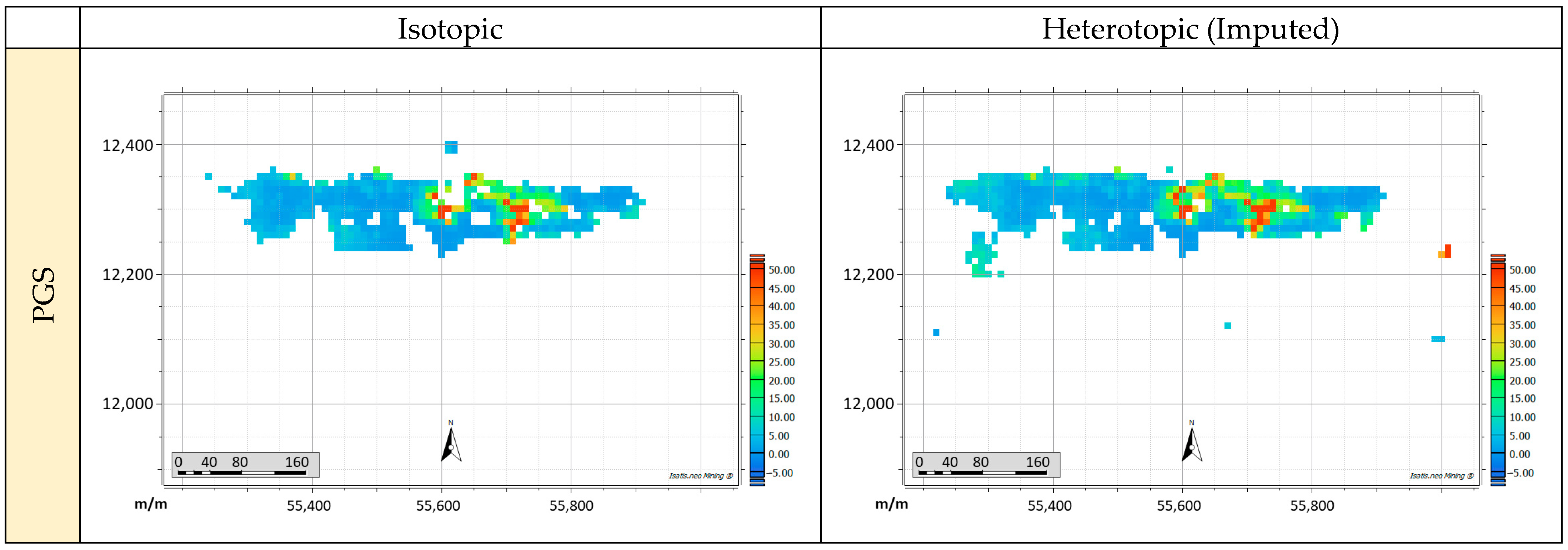
  • PluriGaussian simulation—PGS;
  • Hybrid domaining framework with imbalanced input for the classifier—HDF imbalanced;
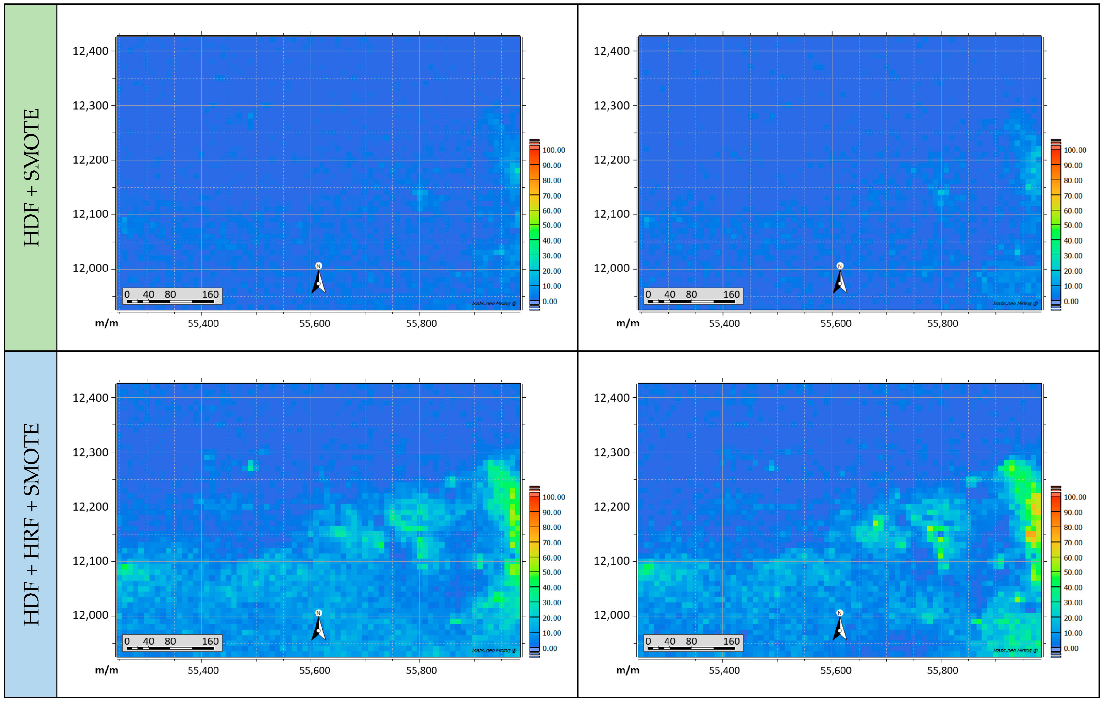
  • Hybrid domaining framework with balanced input for the classifier—HDF + SMOTE;
  • Hybrid domaining framework with noise filtered and balanced input for the classifier—HDF + HRF + SMOTE.

3. Application to a Case Study

3.1. Case Study Overview

The proposed domaining approach is demonstrated in a case study of an Iron Oxide Copper Gold (IOCG) deposit located in Australia. IOCG deposits are mineral deposits that have become increasingly important due to their high economic value and complexity. South Australia is known to have several world-class IOCG deposits, such as the Olympic Dam, Prominent Hill, Carrapateena, and Hillside deposits [50]. IOCG deposits are characterised by their high concentrations of copper, gold, and other valuable metals, such as silver, uranium, and molybdenum [51].
IOCG deposits are typically formed by hydrothermal fluids sourced from deep within the Earth’s crust and deposited in Proterozoic-aged iron oxide-rich sedimentary and volcanic rocks [50]. These fluids deposit metal-rich minerals, such as chalcopyrite, bornite, magnetite, and hematite, in the host rocks, resulting in high-grade ore bodies that can be structurally complex and challenging to mine [51]. Although the complex nature of these deposits presents challenges for exploration and mining, they have been addressed through the development of new techniques and methodologies, such as geometallurgy.
In this case, the geological data contains assay data for numerous elements obtained from drillholes and their corresponding geological features, which have been analysed and interpreted by geologists working at the mine site. For each sample, there are 28 continuous grade variables and one categorical lithology variable. The lithology variable is used to identify domains for the proposed domaining framework. Despite having over 120 unique lithology categories, most of them can be disregarded because they have an insignificant number of samples or can be merged into more significant categories based on their geological features and statistical characteristics. In this study, four major lithology categories obtained by combining 12 major classes (Table 1) and 20 grade assays (Table 2) were used per the mine geologist’s recommendation. The grade variables in Table 2 are considered heterotopic, as assay values for some variables are not available for all samples. The lithology data are imbalanced by major classes such as HMBX, DOLM, and OTHR and minor classes such as HQBX (Table 1). The grade values are based on a composite length of two metres, and the lithology for each sample is selected from the prevailing category within the composite interval. As class OTHR contains several lithological categories, it has broader statistical characteristics, which may overlap with the other three categories. In order to show essential statistical differences between the classes with respect to assay grades, Figure 2 illustrates examples of variables with distinct statistical characteristics. Consequently, continuous and categorical variables are suitable for the classification algorithm of the proposed domaining method, which relies on inter-relationships among the variables.

3.2. PluriGaussian Simulation

The initial stage of PGS requires the definition of the truncation rule and the specification of the threshold values. In this approach, the domains are characterised by truncating a set of Gaussian random fields. The determination of the number of Gaussian random fields, as well as the method of truncation, depends on the contact relationship. In our case, the mine geologist recommended the truncation rule shown in Figure 3.
After determining the threshold values for isotopic and heterotopic data, the indicator data were generated. To determine the variogram models for the Gaussian random fields, experimental variograms were computed for the indicator data in both horizontal and vertical directions. Based on the experimental indicator variograms, the variogram models for the Gaussian random fields were inferred and fitted. It is important to note that the cross-variograms of the Gaussian random fields were assumed to be zero. The fitted Gaussian variograms are shown in Figure 4. The modelled variograms comprised two nested structures (Table 3). Once the variogram models were inferred, the next step involved converting the indicators into Gaussian data using the Gibbs sampler. It involves iteratively assigning categories to locations on a simulation grid based on conditional distributions defined by input data. By considering the spatial characteristics of each category and their interrelationships, the Gibbs sampler produces realistic realisations that capture the complexity and uncertainty of geological systems. Subsequently, 100 realisations were produced and truncated in accordance with the defined truncation rules mentioned above.

3.3. Hybrid Domaining Framework

3.3.1. Modelling and Simulation of Continuous Grade Variables

The PPMT transformation used for the decorrelation process reduces the initial heterotopic dataset of 131 k samples to an isotopic dataset of 93 k samples. This transformation leads to the elimination of the heterotopic portion of the whole dataset, which means disregarding some useful information. However, data imputation can mitigate the issue of unequal sampling, so the complete set of original data can be used for the simulation [44]. In this study, we used the MissForest machine learning-based imputation technique to infer missing values [52]. As a result, by retaining the original number of samples, the heterotopic dataset becomes isotopic. Both isotopic datasets with 131 k and 93 k samples, respectively, are evaluated in terms of domain boundary changes and HDF performance. However, before TBSim is applied, the imputed values are removed because they might be a source of potential bias, thus introducing artificial variability and impacting model performance. In other words, the imputation impacts only the PPMT forward and back transformations and indirectly impacts the simulation results because previously unused information is retained in the domaining process. Therefore, the excluded samples from the isotopic dataset are fully employed in the independent simulation of the heterotopic dataset. Consequently, the uncertainty of the locations with the retained samples is reduced for the corresponding variables.
The cross-correlated variables are transformed into independent Gaussian variables using PPMT. The histograms of six out of the twenty grade variables are presented to provide a better visual understanding of their original distribution (Figure 5). The variables are not segregated by specific criteria such as mineralogy or rock types. Consequently, some grade variables exhibit multi-modal distributions due to the presence of different minerals for the same element. The histograms in Figure 5 show the results of the PPMT transformation examples, which are similar for the remaining transformed variables. Figure 6 displays the bi-variate scatter plots of the original and transformed variables for pairs of grade variables with the most interesting inter-relationships. As can be seen, the example pairs are decorrelated and free from multivariate correlations. This is also the case for the other variables. Consequently, the subsequent steps, including variogram modelling and independent simulations, can be taken.
As previously stated, the simulation step regards the entire region as a stationary zone for variography and assumes the presence of gradual boundaries between lithological domains. It should be noted that the proposed domaining method partitions the region into these domains during the classification step. Following the forward transformation, variogram analyses were conducted on the transformed data, and Table 4 and Table 5 display the resulting fitted variogram models for the isotopic and heterotopic data, respectively. In addition, Figure 7 provides a graphical representation of the variogram models for the transformed Fe variable.
The simulations were generated on a regular grid consisting of 80 × 50 × 65 nodes with a 10-metre grid spacing in all directions. Hereafter, the simulated values of the “blocks” in this case are actually values at the corresponding simulation grid nodes. TBSim was used together with the variogram models in Table 4 and Table 5 to generate 100 realisations for each variable and subset. Once completed, the simulated values were converted back to the original data space. Figure 8 displays the E-type maps, which indicate the average values of 100 realisations for two example variables, Al and Fe, for both the isotopic and heterotopic cases.

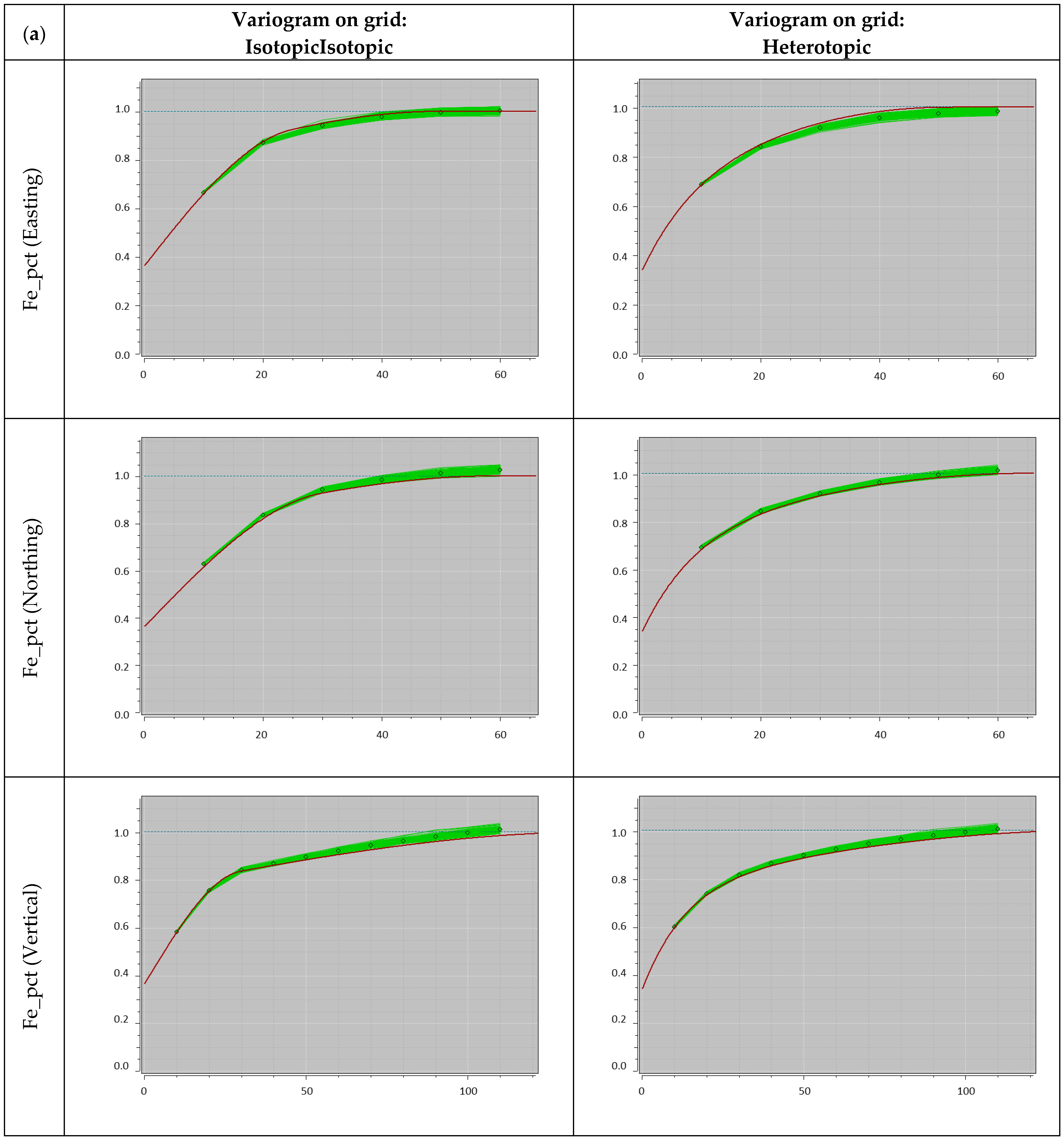
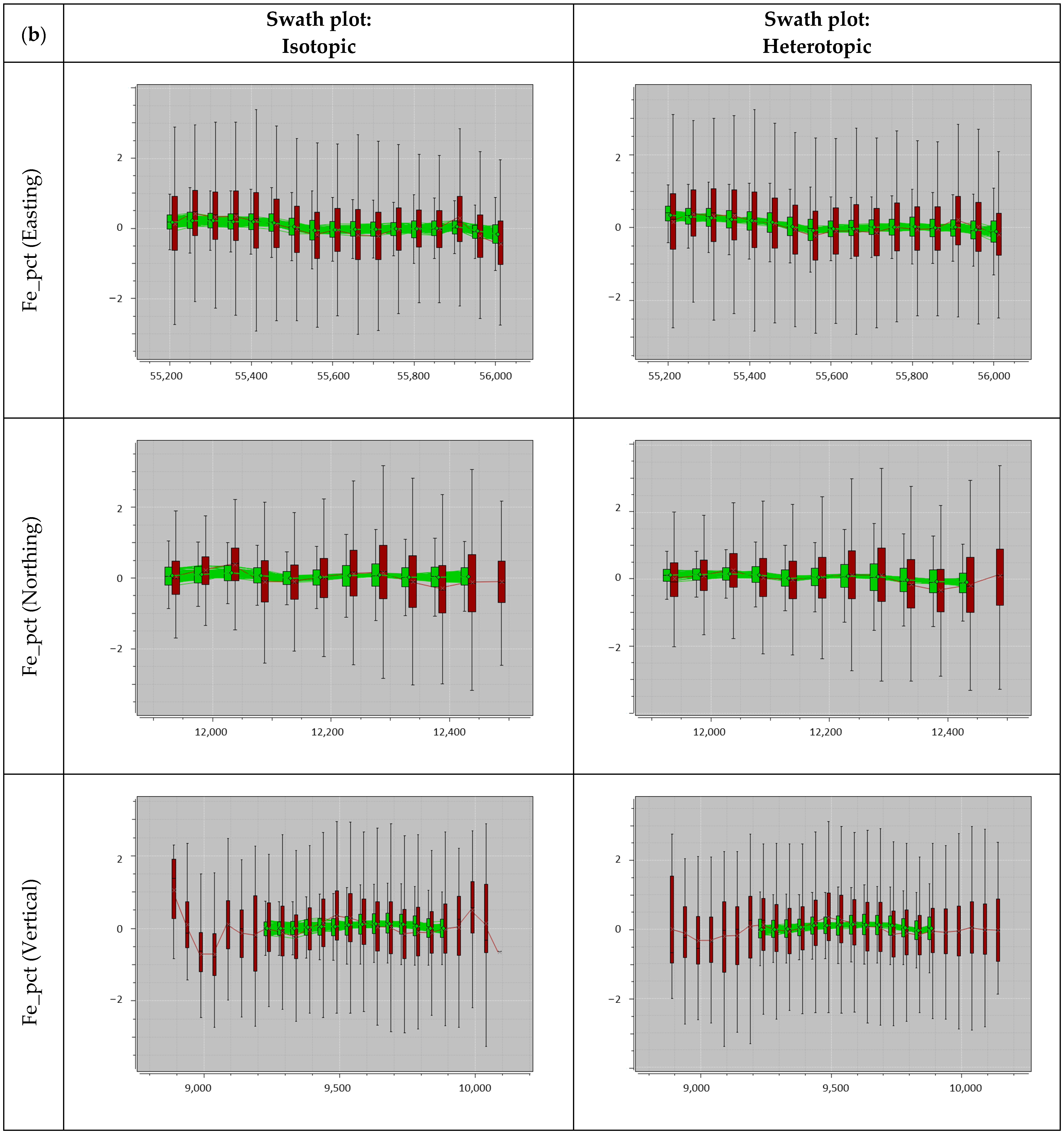
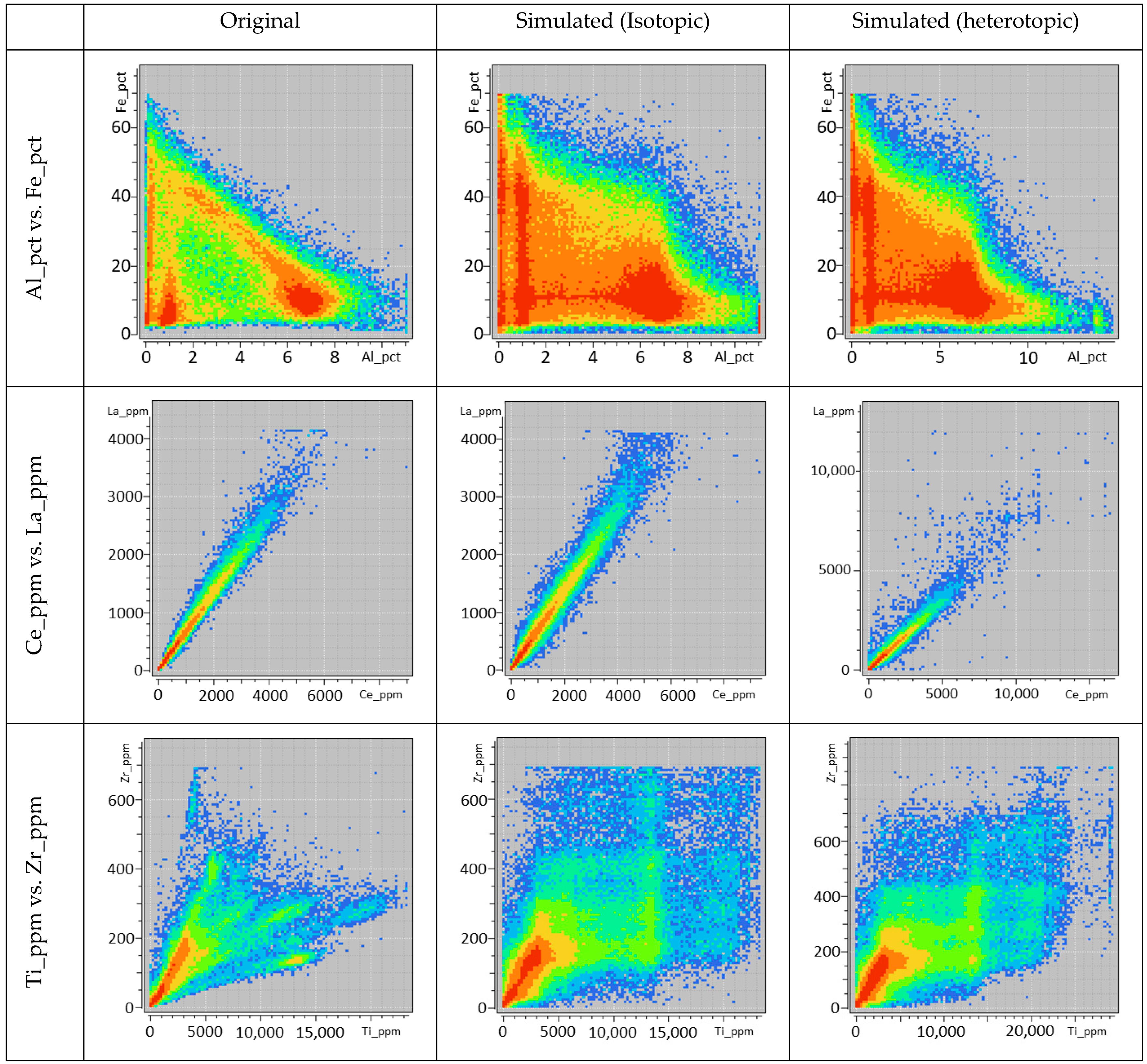
3.3.2. Validation of Simulation Results

The statistical characteristics of the variables, such as global mean and variance, were analysed to assess the accuracy of the simulated grade values. Mean and variance values for each realisation were obtained, and their average values over 100 realisations were compared with the original values, as presented in Table 6. Validation of the local statistical parameters is another way of checking the quality of the simulation results and assessing the reproduction of spatial continuity. The direct variograms of the 100 simulated realisations should be compared with the fitted variogram model [53]. As an illustration, the direct variograms of the Fe variable obtained from TBSim together with the associated models used are shown in Figure 9a, indicating that the spatial continuity is reasonably well reproduced [54]. In addition, Figure 9b depicts swath plots of the grade distributions derived from several directions through the deposit, including East, North, and Vertical directions for the block model and composites. It should be noted that the average values at both ends of the curves are based on a small number of data points (e.g., Figure 9b: swath plot—vertical). A comparison of the simulated values and the original data shows mostly similar results, with some slight deviation observed in the swath plots, which could be due to the strongly skewed distributions of the example variable.
Bivariate scatterplots and correlation coefficients were used to validate the reproduction of the correlations between grade variables. Figure 10 illustrates the bivariate distributions between three example pairs of variables based on their original and simulated values. The overall correlation structures and bivariate distributions were reasonably well reproduced, with the heat maps of the bivariate scatterplots of simulated values being similar to those of the original data. However, certain simulated values (e.g., Ti vs. Zr) did not demonstrate perfect agreement, which may be attributed to the simulation and back-transformation encountering difficulties in managing some multivariate complexities such as heteroscedasticity and other geological constraints in multivariate geostatistical modelling, including unequal sampling, data quality, and scale. It is worth noting that Figure 10 only represents the bivariate scatterplots for one realisation, and all other variables were subjected to the same process of examination to ensure the accuracy of the simulation within the proposed domaining framework.

3.3.3. Preprocessing of Noisy and Misinterpreted Lithology Classes in Samples

The uncertainty associated with the domain boundaries is assessed by the simulation part of the proposed framework, which generates 100 realisations for the assay grades. However, the classification algorithms used in the case study struggle to accurately predict certain lithological classes, such as HQBX and OTHR. Based on discussions with on-site geologists, this difficulty is attributed to the complex geological characteristics and potential errors in the geological core logging process. The extensive and diverse geochemical properties of the OTHR class may correspond to several different combined categories, resulting in incorrect classification of some observations in the dataset. Consequently, the overall rate of misclassification increases. Moreover, distinguishing between HMBX and HQBX poses a challenge, as one can easily be misinterpreted as the other. In fact, a considerable number of HQBX samples are misclassified as HMBX, and this misclassification was identified when examining the overlapping statistical characteristics between the two lithologies [30]. Most of these misclassifications occur in a specific zone in which the block domain model shows HQBX as the second-most likely category after HMBX. However, the expert knowledge of site geologists suggests that the indicated area should contain a significant number of HQBX samples.
Standard machine learning techniques were used to address the problem of incorrect data input by applying noise filtering techniques based on the similarity and dissimilarity of the selected features. In this case study, HRF was employed as an additional step prior to domain classification. As this noise filtering method works only for binary problems, a pairwise approach was used for the multiclass problem. In other words, all possible combinations of pairs among HMBX, HQBX, DOLM, and OTHR classes were processed for the noise filtering. In addition, SMOTE was used to balance each pair to minimise the influence of major classes during the training process. If the balancing is not implemented for highly imbalanced cases, the noise filtering step will be biased towards classes with the highest number of samples [30]. Table 7 provides the statistics of the re-labelled and removed samples in accordance with the corresponding pairs, and Table 8 demonstrates the overall changes of the classes within the isotopic data fed to the XGBoost classifier.

3.3.4. Domain (Lithology) Classification and Uncertainty Quantification

Mine geologists defined the grade domains at the case study mine site based on copper and gold grade values, and the geometries of domain boundaries were manually created. However, due to the subjectivity and uncertainty involved in this approach, a semi-automatic lithological domaining method is of significant interest to the mining operation. Despite the challenges associated with the manual creation of important domains (i.e., HQBX, HMBX, and DOLM), they provide crucial geological information for more precise resource estimation. As a data-driven and semi-automatic approach, the proposed HDF, especially the classification part of the framework, is examined for domain modelling purposes. Thus, XGBoost is trained with several configurations for a better understanding of the classifier’s performance and its impact on the final domain model.
The model training and validation process involves several steps, including splitting the dataset into 70/30 training and testing subsets through stratified resampling followed by stratified 3-fold cross-validation, iterative training of the classifiers with different hyper-parameters, and testing the classifiers for misclassification rates [30]. The isotopic subset of the original dataset is examined here in terms of classifier performances with the noise filtering method, HRF, and balancing algorithm, SMOTE. Table 9 shows the balanced accuracy obtained during the XGBoost training process. The original imbalanced case is the isotopic data without any changes, whereas the original balanced case involves the application of SMOTE prior to the training process in order to reduce bias towards the minor class, HQBX. The noise-filtered balanced case is based on the result obtained in the previous sub-section and balanced by SMOTE before the training process.
In the proposed domaining framework, the outputs of the simulations and the classification model are merged in the final stage. The XGBoost classifier, which has been trained for different cases, is used to forecast the lithology domain at the point level using the simulated values of 20 grade variables, resulting in 100 domain realisations. The most probable outputs for each case are depicted in Figure 11 as examples. It is important to note that XGBoost uses 20 simulated grade values exclusively to predict block lithology without explicitly considering the lithology of neighbouring blocks. In other words, XGBoost does not explicitly use the spatial characteristics of the domain variables and predicts lithology solely based on geochemical characteristics. However, the continuity of the block lithology is implicitly enforced during the grade simulation stage by using soft boundaries for continuous grade variables. This results in the spatial connectivity being indirectly accounted for in the final lithology prediction.
A total of 100 realisations were used to assess the uncertainty in the estimated block domains. The most probable model for block lithology is determined by identifying the domain category with the highest probability for each block. The probability of a block belonging to a domain can be calculated as the proportion of predicted lithology out of the 100 realisations. Figure 12 illustrates the corresponding highest probability of the most likely domain for the cross-section shown in Figure 11. These maps quantify the uncertainty associated with the prediction of the most probable block lithology model.

3.4. Post-Processing the Realisations: Geometallurgical Domains

The use of realisation outcomes from HDF can assist in making informed decisions in a mining project. A significant benefit of this process is the ability to provide reliable domain boundaries with the corresponding probabilities, which will assist in correctly identifying mineral processing destinations for mined blocks. Simulation methods are used to estimate the uncertainty associated with domain boundaries and to identify areas with higher probability in relation to processing responses, such as NSR and grinding time. These areas can be regarded as geometallurgical domains that exhibit a certain level of confidence in decision-making processes related to mined blocks. Hence, this sub-section compares PGS and HDF in terms of two geometallurigcal models: NSR and grinding time.

3.4.1. Net Smelter Return

The NSR cut-off, which is used to determine the economic viability of a mining project, considers the revenue generated from copper and gold metals as well as the costs associated with mining operations, mineral processing, capital, and any penalty elements (in this case, fluorine and uranium). The NSR calculation also takes into account the estimated metallurgical recoveries of the minerals. In order to determine the NSR value for each block, metal recovery rates were estimated based on the expected sulphide mineralogy (for copper) or grade (for gold and silver) of each block. These recovery rates were derived using empirical models based on the processing plant performance. The block-by-block approach ensures that the NSR calculation accurately reflects the expected revenue generated from each individual block and helps to identify economically viable sections of the orebody. NSR values are calculated within the DOLM domain as it is most likely to contain gold and copper for the detailed analysis. The following simplified NSR formula was used to calculate the final results:
N S R s i m p l i f i e d = A × A u p p m + B × C u p c t C × F p c t D × U p p m
where, A, B, C, and D are factors that depend on revenue, refining charges, metallurgical recovery assumptions, transport costs, and taxes. The most probable output for the DOLM domain was obtained from the PGS and HDF approaches chosen for the simulation of Au and Cu components and the deleterious F and U elements. Subsequently, the NSR is calculated using the following equation:
N S R s i m p l i f i e d = 1.15 × A u p p m + 29.4 × C u p c t 0.51 × F p c t 0.0064 × U p p m
The E-type maps in Figure 13, Figure 14 and Figure 15 represent the geometallurgical model for NSR values within the DOLM lithological domain over 100 conditional realisations, indicating areas with varying levels of certainty in finding particular geometallurgical domain boundaries. The blue sectors on the map represent areas with little profit, while the red sectors denote areas with a high level of potential profit. However, it is important to note that these descriptions are for average-case scenarios. The worst- and best-case scenarios can be found by taking into account the particular domain boundaries and grade realisations from the simulation results.

3.4.2. Grinding Time

One critical aspect of mining is the process of reducing the size of the extracted materials by grinding. Grinding is an energy-intensive process that accounts for a significant portion of the total energy consumption in mining operations. The amount of grinding required has a direct impact on energy efficiency, throughput, and the overall profitability of a mining operation. Thus, understanding the factors that contribute to grinding time is essential for optimising the process and improving the economic viability of mining operations.
The factors that influence grinding time include the ore type, the size distribution of the crushed ore, the hardness of the ore, the grinding process, and the operating conditions. These factors can impact the grinding efficiency, which is typically measured by the amount of material that can be ground per unit of energy consumed. In this case study, HMBX and HQBX domains have significant differences in grinding time, although it is easy to misclassify these two lithologies during the core logging process. The HQBX composited ore requires 1.5–1.8 times more time to grind than ore with HMBX content. Thus, the prediction of the boundaries of these two domains is critical, as the lithological model, especially the HQBX domain, is directly related to geometallurigcal responses such as grinding time.
In the most probable maps shown above, differences in the presence of HQBX and HMBX may vary depending on each domaining method. As a result, the grinding time for particular blocks may differ. Assuming that the general conditions are similar for HQBX and HMBX, a comparison in terms of the number of blocks per domain shows the extent to which the grinding time can change from one method to another (Table 10). As a result, noise filtering significantly affects the final outcome for the HQBX class, and thus grinding time is likely to be longer for some of the mining blocks. Consequently, decisions related to processing require revision.

4. Results and Discussion

The proposed domaining framework includes the HybridRepairFilter noise filtering method, which has resulted in a significant change in the domain layout. The filtering involves the removal of 2029 samples and the re-labelling of 1953 samples from the original HMBX class to the HQBX class. When the preprocessing is implemented, there is a significant increase in the number of blocks classified as HQBX, as shown in Table 11. Without preprocessing, none of the blocks were classified as HQBX lithology. Moreover, the singular balancing by SMOTE, excluding noise filtering, resulted in 2 or 3 HQBX blocks for the isotopic or heterotopic data. The number of HQBX blocks increased to 4945 for the isotopic subset and to 6286 for the heterotopic subset when noise filtering preprocessing was used. The use of the multiclass HRF noise filtering method resulted in significant changes in the HMBX and HQBX domains. Other domains have slight changes, which can be seen in the most probable results in Table 11.
The proposed domaining framework may be impacted by three main sources of uncertainty related to the domain boundary definition. The first source is the inherent uncertainty associated with the data, which can result in significant errors due to mis-logging. While data uncertainty cannot be completely eliminated, it can be reduced through noise filtering for important domains such as HMBX and HQBX. The second source of uncertainty comes from the simulation results, which can be used to generate multiple realisations for uncertainty quantification. Finally, there is model’s uncertainty associated with the classification algorithm and the SMOTE balancing method, which relies heavily on input data to produce reliable outputs. This classification model uncertainty is directly influenced by the previous two sources of uncertainty. As a consequence, the proposed domaining framework can be impacted by multiple sources of uncertainty, and reducing these impacts requires each of these sources to be assessed. In this case, the probability maps can be used to mitigate the risk associated with the overall uncertainty in the generated domain boundaries. Using thresholds, blocks with high certainty can be selected for further resource classification.

4.1. Geometallurgical Model: Net Smelter Return

A NSR cut-off and specific mining dimensions may be used to optimise stope layouts. The optimisation process is informed by the local orientation of the interpreted mineralization zone, with high grades commonly represented using wireframes (i.e., triangulations). Consequently, some material below the specified cut-off grade may be included, and some material above the cut-off value may be excluded during future extraction. In this study, the calculated NSR is relative to the original NSR used on the mine site, which is based on the revenue generated from the extracted metals and the expenses incurred in site operations. The NSR was computed for the DOLM domain produced by PGS and HDF with different configurations.
In the maps shown in Section 3.4.1, the general DOLM domain boundaries are similar for all the methods. However, the probabilities of PGS and HDF are significantly different because the DOLM boundaries shrink rapidly as the threshold for the domain probability approaches its maximum. For example, when the DOLM domain for predicting NSR is set to a probability of 70% (P-70), the number of HDF blocks decreases to more than twice that with a probability of 50% (P-50), whereas the number of blocks for PGS decreases by about 1.5 times (Table 12). The overall mean values for NSR stay relatively stable for all the corresponding thresholds (cut-offs), which is expected for the DOLM class because of its distinct geochemical characteristics. Consequently, HDF and PGS produce similar results for the geometallurgical model of NSR values.

4.2. Geometallurgical Model: Grinding Time—HQBX

The grinding times for HMBX and HQBX may differ due to the differences in their physical and chemical properties. HQBX contains quartz in addition to hematite, while HMBX contains only hematite. Quartz is a harder mineral than hematite, which means that Hematite Quartz Breccia requires a longer grinding time to achieve the desired particle size compared with Hematite Breccia.
According to the mine geologists and actual processing (i.e., grinding) results, it takes around 5–6 min for a unit of HMBX and 9–11 min for a unit of HQBX to be ground to the desired particle size and quality. The number of blocks for HQBX varies significantly for the PGS and HDF domaining methods. In Table 13, the results for PGS reproduce the original HQBX proportions for isotopic and heterotopic data. As a result, there is a good HQBX presence. However, classifiers in the case of HDF with imbalanced and balanced (i.e., SMOTE) completely disregard the HQBX in their prediction. The reasons behind this are the low number of HQBX samples, the inherent noise in the data, and the similarity of the HQBX and HMBX classes. On the other hand, HRF solves the problem of noisy data and provides distinct statistical boundaries for the classifier [30]. Consequently, the balanced HDF with HRF predicts many more blocks than PGS because it depends on the simulated grade values (Figure 16) and not directly on the domain proportions of samples. This is advantageous for irregularly spaced data, such as in this case study.

4.3. General Performance

The outcomes derived from the proposed HDF domaining framework demonstrate considerable potential, particularly in situations that involve unbalanced datasets. The framework can accommodate a higher number of domains and can differentiate domains that appear to be almost identical classes/domains, such as HMBX and HQBX, by using noise-filtering approaches. Abildin et al. [30] demonstrated the application of the HDF for a multiclass problem, but with the HRF applied for the binary class. In this paper, HRF is used for the multiclass problem using the pairwise approach, in which noise for each class is filtered out against all other classes. A comparison of the most probable PGS and HDF maps for the DOLM domain shows that the domain boundaries are similar, although the probabilities are different. In the case of the HQBX domain, the reproduction of the class is different, but the most probable maps show similar features in the same locations. Thus, the geometallurgical model for NSR is similar to that of PGS and the modified HDF. However, the reproduction of the geometallurgical model for HQBX is better for the HDF, as demonstrated in the validation in Abildin et al. [30]. Overall, for stable domains, such as DOLM, the geometallurgical models produced by the modified HDF are similar to the models obtained by benchmarking PGS. HDF can handle complex geometallurgical domains such as HQBX by including quantitated covariates.
The use of HDF provides the added advantage of quantifying the level of uncertainty associated with the domain model, as can be seen in the analyses provided in this paper. Moreover, it incorporates more abundant grade values into the domaining process, and thus, the reliability of the domain boundaries increases. HRF and SMOTE mitigate data problems such as noise and imbalance. The benefit of using all important information significantly impacts the evaluation of confidence in the resource model as it enables more accurate classification of resource categories based on the JORC code [55].

5. Conclusions

The accurate definition of domains is critical for the estimation of mineral resources. The current practises for domaining include labour-intensive explicit modelling, complex implicit modelling, and tedious geostatistical methods such as PluriGaussian simulation. To address these challenges, the authors previously proposed a hybrid data-driven machine learning-based domaining framework (HDF) that combines geostatistical simulations and classification algorithms with noise filtering preprocessing (HRF). HDF is data-driven, using only grade data and lithology logs to define domain boundaries. In this work, the method has been compared with PGS, which simulates categorical variables by using the truncation rule on Gaussian random fields.
HDF and PGS have been tested using a dataset from an IOCG deposit that has complex geological features. The proposed domaining method uses the turning bands method for simulations, an extreme gradient boosting classification algorithm for classification, and an ensemble of machine learning methods for noise removal for the multiclass problem and detection of potentially miss-logged domain categories. The preprocessing of data has been demonstrated to enhance the performance of the classification algorithm, leading to better results produced by the domaining framework. The proposed method generates a block-domain model with multiple realisations, from which the most likely block-domain model and the corresponding probability can be obtained to quantify uncertainty. The impacts of the produced domain boundaries on the geometallurgical models, such as NSR and grinding time, are further examined in this work.
HDF is a versatile approach that can be applied to other datasets originating from diverse deposits and is not restricted to the modelling of lithological variables. This framework can be extended to model any categorical variable that depends on continuous variables, such as the geometallurgical domains investigated in this study. By using this method, it is anticipated that the accuracy of mineral resource estimation will be enhanced, resulting in increased confidence in the location and quantity of valuable minerals.

Author Contributions

Y.A.: Conceptualisation, Methodology, Software, Validation, Investigation, Writing—Original Draft, Writing—Review & Editing, Visualisation. C.X., P.D. and A.A.: Conceptualisation, Methodology, Resources, Writing—Review & Editing, Supervision. All authors have read and agreed to the published version of the manuscript.

Funding

This research has been supported by the South Australian Government through the PRIF RCP Mining Consortium “Unlocking Complex Resources through Lean Processing”.

Data Availability Statement

Data is not allowed to share since it has sensitive information.

Acknowledgments

The authors thank the Geovariances Company for providing their software for academic use.

Conflicts of Interest

The authors declare that they have no known competing financial interests or personal relationships that could have appeared to influence the work reported in this paper.

References

  1. Coward, S.; Dowd, P. Geometallurgical models for the quantification of uncertainty in mining project value chains. In Proceedings of the International Symposium on the Application of Computers and Operations Research in the Mineral Industry (APCOM), Fairbanks, AK, USA, 23–27 May 2015; pp. 360–369. [Google Scholar]
  2. Macfarlane, A.; Williams, T. Optimizing value on a copper mine by adopting a geometallurgical solution. J. South. Afr. Inst. Min. Metall. 2014, 114, 929–935. [Google Scholar]
  3. Tercan, A.; Sohrabian, B. Multivariate geostatistical simulation of coal quality data by independent components. Int. J. Coal Geol. 2013, 112, 53–66. [Google Scholar] [CrossRef]
  4. Dowd, P.; Xu, C.; Coward, S. Strategic mine planning and design: Some challenges and strategies for addressing them. Min. Technol. 2016, 125, 22–34. [Google Scholar] [CrossRef]
  5. Lishchuk, V.; Koch, P.-H.; Ghorbani, Y.; Butcher, A.R. Towards integrated geometallurgical approach: Critical review of current practices and future trends. Miner. Eng. 2020, 145, 106072. [Google Scholar] [CrossRef]
  6. Deutsch, J.; Szymanski, J.; Etsell, T. Metallurgical variable re-expression for geostatistics. In Geostatistical and Geospatial Approaches for the Characterization of Natural Resources in the Environment: Challenges, Processes and Strategies; Springer International Publishing: Berlin/Heidelberg, Germany, 2016; pp. 83–88. [Google Scholar]
  7. Abildin, Y.; Madani, N.; Topal, E. A hybrid approach for joint simulation of geometallurgical variables with inequality constraint. Minerals 2019, 9, 24. [Google Scholar] [CrossRef] [Green Version]
  8. Adeli, A.; Dowd, P.; Emery, X.; Xu, C. Using cokriging to predict metal recovery accounting for non-additivity and preferential sampling designs. Miner. Eng. 2021, 170, 106923. [Google Scholar] [CrossRef]
  9. Sepulveda, E.; Dowd, P.; Xu, C.; Addo, E. Multivariate modelling of geometallurgical variables by projection pursuit. Math. Geosci. 2017, 49, 121–143. [Google Scholar] [CrossRef]
  10. Cowan, E.; Beatson, R.; Ross, H.; Fright, W.; McLennan, T.; Evans, T.; Carr, J.; Lane, R.; Bright, D.; Gillman, A. Practical implicit geological modelling. In Proceedings of the 5th International Mining Geology Conference, Bendigo, VIC, Australia, 17–19 November 2003; pp. 89–99. [Google Scholar]
  11. Gonçalves, Í.G.; Kumaira, S.; Guadagnin, F. A machine learning approach to the potential-field method for implicit modeling of geological structures. Comput. Geosci. 2017, 103, 173–182. [Google Scholar] [CrossRef]
  12. Lajaunie, C.; Courrioux, G.; Manuel, L. Foliation fields and 3D cartography in geology: Principles of a method based on potential interpolation. Math. Geol. 1997, 29, 571–584. [Google Scholar] [CrossRef]
  13. Manchuk, J.G.; Deutsch, C.V. Boundary modeling with moving least squares. Comput. Geosci. 2019, 126, 96–106. [Google Scholar] [CrossRef]
  14. Armstrong, M.; Galli, A.; Beucher, H.; Loc’h, G.; Renard, D.; Doligez, B.; Eschard, R.; Geffroy, F. Plurigaussian Simulations in Geosciences; Springer Science & Business Media: Berlin/Heidelberg, Germany, 2011. [Google Scholar]
  15. Emery, X.; Séguret, S.A. Geostatistics for the Mining Industry: Applications to Porphyry Copper Deposits; CRC Press: Boca Raton, FL, USA, 2020. [Google Scholar]
  16. Journel, A.; Isaaks, E. Conditional indicator simulation: Application to a Saskatchewan uranium deposit. J. Int. Assoc. Math. Geol. 1984, 16, 685–718. [Google Scholar] [CrossRef]
  17. Journel, A.G. Nonparametric estimation of spatial distributions. J. Int. Assoc. Math. Geol. 1983, 15, 445–468. [Google Scholar] [CrossRef]
  18. Xu, C.; Dowd, P.A.; Mardia, K.V.; Fowell, R.J. A flexible true plurigaussian code for spatial facies simulations. Comput. Geosci. 2006, 32, 1629–1645. [Google Scholar] [CrossRef]
  19. Emery, X.; Ortiz, J.; Cáceres, A. Geostatistical modelling of rock type domains with spatially varying proportions: Application to a porphyry copper deposit. J. South. Afr. Inst. Min. Metall. 2008, 108, 284–292. [Google Scholar]
  20. Maleki, M.; Emery, X.; Cáceres, A.; Ribeiro, D.; Cunha, E. Quantifying the uncertainty in the spatial layout of rock type domains in an iron ore deposit. Comput. Geosci. 2016, 20, 1013–1028. [Google Scholar] [CrossRef]
  21. Silva, D. Enhanced Geologic Modeling of Multiple Categorical Variables. Ph.D. Thesis, University of Alberta, Edmonton, AB, Canada, 2018. [Google Scholar]
  22. Séguret, S.A. Analysis and estimation of multi-unit deposits: Application to a porphyry copper deposit. Math. Geosci. 2013, 45, 927–947. [Google Scholar] [CrossRef] [Green Version]
  23. Adeli, A.; Emery, X.; Dowd, P. Geological modelling and validation of geological interpretations via simulation and classification of quantitative covariates. Minerals 2017, 8, 7. [Google Scholar] [CrossRef] [Green Version]
  24. Fouedjio, F.; Hill, E.J.; Laukamp, C. Geostatistical clustering as an aid for ore body domaining: Case study at the Rocklea Dome channel iron ore deposit, Western Australia. Appl. Earth Sci. 2018, 127, 15–29. [Google Scholar] [CrossRef]
  25. Madani, N.; Maleki, M.; Emery, X. Nonparametric geostatistical simulation of subsurface facies: Tools for validating the reproduction of, and uncertainty in, facies geometry. Nat. Resour. Res. 2019, 28, 1163–1182. [Google Scholar] [CrossRef]
  26. Moreira, G.d.C.; Coimbra Leite Costa, J.F.; Marques, D.M. Defining geologic domains using cluster analysis and indicator correlograms: A phosphate-titanium case study. Appl. Earth Sci. 2020, 129, 176–190. [Google Scholar] [CrossRef]
  27. Sepúlveda, E.; Dowd, P.; Xu, C. Fuzzy clustering with spatial correction and its application to geometallurgical domaining. Math. Geosci. 2018, 50, 895–928. [Google Scholar] [CrossRef] [Green Version]
  28. Kasmaee, S.; Raspa, G.; de Fouquet, C.; Tinti, F.; Bonduà, S.; Bruno, R. Geostatistical estimation of multi-domain deposits with transitional boundaries: A sensitivity study for the Sechahun iron mine. Minerals 2019, 9, 115. [Google Scholar] [CrossRef] [Green Version]
  29. Amarante, F.A.N.; Rolo, R.M.; Coimbra Leite Costa, J.F. Boundary simulation–a hierarchical approach for multiple categories. Appl. Earth Sci. 2021, 130, 114–130. [Google Scholar] [CrossRef]
  30. Abildin, Y.; Xu, C.; Dowd, P.; Adeli, A. A hybrid framework for modelling domains using quantitative covariates. Appl. Comput. Geosci. 2022, 16, 100107. [Google Scholar] [CrossRef]
  31. Adeli, A.; Emery, X. Geostatistical simulation of rock physical and geochemical properties with spatial filtering and its application to predictive geological mapping. J. Geochem. Explor. 2021, 220, 106661. [Google Scholar] [CrossRef]
  32. Rossi, M.E.; Deutsch, C.V. Mineral Resource Estimation; Springer Science & Business Media: Berlin/Heidelberg, Germany, 2013. [Google Scholar]
  33. Matheron, G.; Beucher, H.; de Fouquet, C.; Galli, A.; Guérillot, D.; Ravenne, C. Conditional simulation of the geometry of fluvio-deltaic reservoirs. In Proceedings of the SPE Annual Technical Conference and Exhibition, Dallas, TX, USA, 27–30 September 1987. [Google Scholar]
  34. Sadeghi, M.; Madani, N.; Falahat, R.; Sabeti, H.; Amini, N. Hierarchical reservoir lithofacies and acoustic impedance simulation: Application to an oil field in SW of Iran. J. Pet. Sci. Eng. 2022, 208, 109552. [Google Scholar] [CrossRef]
  35. Dowd, P.; Pardo-Igúzquiza, E.; Xu, C. Plurigau: A computer program for simulating spatial facies using the truncated plurigaussian method. Comput. Geosci. 2003, 29, 123–141. [Google Scholar] [CrossRef]
  36. Madani, N.; Emery, X. Plurigaussian modeling of geological domains based on the truncation of non-stationary Gaussian random fields. Stoch. Environ. Res. Risk Assess. 2017, 31, 893–913. [Google Scholar] [CrossRef]
  37. Emery, X.; Lantuéjoul, C. Tbsim: A computer program for conditional simulation of three-dimensional gaussian random fields via the turning bands method. Comput. Geosci. 2006, 32, 1615–1628. [Google Scholar] [CrossRef]
  38. Le Loc’h, G.; Galli, A. Truncated plurigaussian method: Theoretical and practical points of view. Geostat. Wollongong 1997, 96, 211–222. [Google Scholar]
  39. Emery, X. Simulation of geological domains using the plurigaussian model: New developments and computer programs. Comput. Geosci. 2007, 33, 1189–1201. [Google Scholar] [CrossRef]
  40. Lantuéjoul, C. Geostatistical Simulation: Models and Algorithms; Springer Science & Business Media: Berlin/Heidelberg, Germany, 2001. [Google Scholar]
  41. Arroyo, D.; Emery, X. Spectral simulation of vector random fields with stationary Gaussian increments in d-dimensional Euclidean spaces. Stoch. Environ. Res. Risk Assess. 2017, 31, 1583–1592. [Google Scholar] [CrossRef]
  42. Emery, X. A turning bands program for conditional co-simulation of cross-correlated Gaussian random fields. Comput. Geosci. 2008, 34, 1850–1862. [Google Scholar] [CrossRef]
  43. Friedman, J.H.; Tukey, J.W. A projection pursuit algorithm for exploratory data analysis. IEEE Trans. Comput. 1974, 100, 881–890. [Google Scholar] [CrossRef]
  44. Barnett, R.M.; Manchuk, J.G.; Deutsch, C.V. Projection pursuit multivariate transform. Math. Geosci. 2014, 46, 337–359. [Google Scholar] [CrossRef]
  45. Chen, T.; Guestrin, C. XGBoost: A scalable tree boosting system. In Proceedings of the 22nd ACM SIGKDD International Conference on Knowledge Discovery and Data Mining, San Francisco, CA, USA, 13–17 August 2016; pp. 785–794. [Google Scholar]
  46. Gu, Y.; Zhang, D.; Bao, Z. Lithological classification via an improved extreme gradient boosting: A demonstration of the Chang 4+ 5 member, Ordos Basin, Northern China. J. Asian Earth Sci. 2021, 215, 104798. [Google Scholar] [CrossRef]
  47. Morales, P.; Luengo, J.; Garcia, L.P.F.; Lorena, A.C.; de Carvalho, A.C.; Herrera, F. The NoiseFiltersR Package: Label Noise Preprocessing in R. R J. 2017, 9, 219. [Google Scholar] [CrossRef] [Green Version]
  48. Miranda, A.L.; Garcia, L.P.F.; Carvalho, A.C.; Lorena, A.C. Use of classification algorithms in noise detection and elimination. In Proceedings of the Hybrid Artificial Intelligence Systems: 4th International Conference, HAIS 2009, Salamanca, Spain, 10–12 June 2009; pp. 417–424. [Google Scholar]
  49. Fernández, A.; Garcia, S.; Herrera, F.; Chawla, N.V. SMOTE for learning from imbalanced data: Progress and challenges, marking the 15-year anniversary. J. Artif. Intell. Res. 2018, 61, 863–905. [Google Scholar] [CrossRef]
  50. Williams, P.J.; Barton, M.D.; Johnson, D.A.; Fontboté, L.; De Haller, A.; Mark, G.; Oliver, N.H.; Marschik, R. Iron oxide copper-gold deposits: Geology, space-time distribution, and possible modes of origin. Econ. Geol. 2005, 100, 371–405. [Google Scholar] [CrossRef]
  51. Belperio, A.; Flint, R.; Freeman, H. Prominent Hill: A hematite-dominated, iron oxide copper-gold system. Econ. Geol. 2007, 102, 1499–1510. [Google Scholar] [CrossRef]
  52. Stekhoven, D.J.; Bühlmann, P. MissForest—Non-parametric missing value imputation for mixed-type data. Bioinformatics 2012, 28, 112–118. [Google Scholar] [CrossRef] [PubMed] [Green Version]
  53. Emery, X. Testing the correctness of the sequential algorithm for simulating Gaussian random fields. Stoch. Environ. Res. Risk Assess. 2004, 18, 401–413. [Google Scholar] [CrossRef]
  54. Leuangthong, O.; McLennan, J.A.; Deutsch, C.V. Minimum acceptance criteria for geostatistical realizations. Nat. Resour. Res. 2004, 13, 131–141. [Google Scholar] [CrossRef]
  55. Code, J. Australasian code for reporting of exploration results, mineral resources and ore reserves. AusIMM Melb. 2012, 44, 320. [Google Scholar]
Figure 1. Brief workflow for PGS steps.
Minerals 13 00918 g001
Figure 2. Standardised boxplots for the variables grouped by lithological categories.
Minerals 13 00918 g002aMinerals 13 00918 g002bMinerals 13 00918 g002c
Figure 3. Truncation rule for the lithologies while maintaining the relative proportions.
Minerals 13 00918 g003
Figure 4. Gaussian variogram models: the experimental variograms are indicated by points and the fitted models ((a,c)—Isotopic; (b,d)—Heterotopic) are the solid lines in the East (red), the North (green) and the vertical (blue) directions. (a) Y(Isotopic—1). (b) Y(Heterotopic—1). (c) Y(Isotopic—2). (d) Y(Heterotopic—2).
Minerals 13 00918 g004aMinerals 13 00918 g004b
Figure 5. Histograms examples of six grade assay variables: original heterotopic, isotopic, standard Gaussian and PPMT transformed factors based on the isotopic subset (pct—percentage, ppm—parts per million).
Minerals 13 00918 g005aMinerals 13 00918 g005b
Figure 6. Bivariate scatterplots of Al vs. Fe, Ce vs. La, and Ti vs. Zr of original (left), Gaussian (centre) and PPMT transformation (right) (G[]—Gaussian, P[]—PPMT factor, pct—percentage, ppm—parts per million).
Minerals 13 00918 g006aMinerals 13 00918 g006b
Figure 7. Variogram models of an example variable, Fe_pct(PPMT), for both the isotopic (left) and heterotopic (right) cases. The experimental variograms are indicated by points and the fitted models by a solid line along the East (red), the North (green) and Vertical (blue) directions (pct—percentage, ppm—parts per million).
Minerals 13 00918 g007
Figure 8. Top view of the cross-section of the average value of 100 realisations for isotopic and heterotopic cases of Al and Fe at the elevation Z = 9715 m.
Minerals 13 00918 g008
Figure 9. Cross-validation of the original values of Al and Fe: (a) variogram of simulated values on the grid (red line—fitted variogram model; green lines and dots—variograms and their mean on the grid) and (b) swath plots for (left) isotopic and (right) heterotopic data in the East, North and Vertical directions (red—original values; green—simulated realisations).
Minerals 13 00918 g009aMinerals 13 00918 g009b
Figure 10. Bivariate scatterplots of Al vs. Fe, Ce vs. La, and Ti vs. Zr for the original (left) values, and back-transformed simulated values on the isotopic subset (centre) and heterotopic subset (right) of Realisation 1 (pct—percentage, ppm—parts per million).
Minerals 13 00918 g010
Figure 11. Top view of the horizontal cross-section for the most probable lithological model at an Elevation of Z = 9715 m.
Minerals 13 00918 g011aMinerals 13 00918 g011b
Figure 12. Top view of the horizontal cross-sections for the probability of the most probable domain at an elevation of Z = 9715 m.
Minerals 13 00918 g012aMinerals 13 00918 g012b
Figure 13. Top view of the horizontal cross-sections for the NSR with the most probable DOLM domain at an elevation of Z = 9715 m.
Minerals 13 00918 g013aMinerals 13 00918 g013b
Figure 14. Top view of the horizontal cross-sections for the NSR with 50% probability of the DOLM domain at an elevation of Z = 9715 m.
Minerals 13 00918 g014
Figure 15. Top view of the horizontal cross-sections for the NSR with 70% probability of the DOLM domain at an elevation of Z = 9715 m.
Minerals 13 00918 g015aMinerals 13 00918 g015b
Figure 16. Top view of the horizontal cross-sections for HQBX probability at an elevation of Z = 9715 m.
Minerals 13 00918 g016aMinerals 13 00918 g016b
Table 1. Brief description and statistical characteristics of the lithologies.
No.CategoryNameHeterotopic DataIsotopic Data
Number of SamplesProportion (%)Number of SamplesProportion (%)
1HMBXHematite Breccia37,75528.7425,96628.01
2HQBXHematite Quartz Breccia35102.6711821.27
3DOLMDolomite31,50623.9925,80927.84
4OTHRAll other classes58,57444.6039,74942.88
Table 2. Brief description and statistical characteristics of the grade assays (pct—percentage, ppm—parts per million).
No.AbbreviationDescription Number of SamplesMin.Max.MeanVariance
1Al_pctAluminium 125,7790.014.83.747.34
2Au_ppmGold131,3430.0137.60.341.58
3Ba_pctBarium131,2610.013.10.310.38
4Ca_pctCalcium128,0360.027.24.1230.6
5Ce_ppmCerium131,3102.01.7 × 104817.808.2 × 105
6Cr_ppmChromium131,2611.01.6 × 10362.796.4 × 103
7Cu_pctCopper131,3450.020.60.40.89
8F_pctFluorine102,7860.013.20.270.15
9Fe_pctIron131,3110.469.519.87165.4
10K_ppmPotassium131,064258.6 × 1041.8 × 1042.0 × 108
11La_ppmLanthanum131,2582.01.2 × 1045.5 × 1023.9 × 105
12Mg_ppmMagnesium131,261251.7 × 1052.8 × 1049.5 × 108
13Mn_ppmManganese128,245103.3 × 1042.3 × 1038.8 × 106
14Na_ppmSodium131,261206.0 × 1041.5 × 1031.8 × 107
15P_ppmPhosphorus131,2612.55.5 × 1041.3 × 1031.2 × 106
16S_pctSulphur127,7990.015.30.370.30
17Si_pctSilicon125,6530.144.918.5664.4
18Ti_ppmTitanium131,2615.02.9 × 1043.7 × 1031.4 × 107
19Zn_ppmZinc131,3451.01.0 × 10435.44.7 × 103
20Zr_ppmZirconium93,1002.5862.5125.31.0 × 104
Table 3. Parameters of the fitted Gaussian variograms models.
No. Gaussian Random FieldNuggetStructure 1Structure 2
ca (EW), ma (NS), ma (vert), mca (EW), ma (NS), ma (vert), m
a γ Isotopic 1 00.30 Sph3090300.70 Sph25090300
c γ Isotopic 2 00.40 Sph3090600.60 Sph330150300
b γ Heterotopic 1 00.30 Gauss5050700.70 Cub400130450
d γ Heterotopic 2 00.40 Exp5050500.60 Exp330170300
Table 4. Fitted variogram models for the grade assay variables for the isotopic subset (pct—percentage, ppm—parts per million).
No. Grade VariableNuggetStructure 1Structure 2
ca (EW), ma (NS), ma (vert), mca (EW), ma (NS), ma (vert), m
1 γ A l P P M T _ G a u s s 0.400.452517240.15500324500
2 γ A u P P M T _ G a u s s 0.450.483433410.07274500176
3 γ B a P P M T _ G a u s s 0.410.322137390.2713067130
4 γ C a P P M T _ G a u s s 0.320.382231430.30500207222
5 γ C e P P M T _ G a u s s 0.340.402017260.2620392188
6 γ C r P P M T _ G a u s s 0.400.442018260.16289120380
7 γ C u P P M T _ G a u s s 0.280.493242510.231405090
8 γ F P P M T _ G a u s s 0.240.421919230.34180112184
9 γ F e P P M T _ G a u s s 0.360.402530300.245059140
10 γ K P P M T _ G a u s s 0.250.511814180.2410756184
11 γ L a P P M T _ G a u s s 0.430.392021280.18351303500
12 γ M g P P M T _ G a u s s 0.350.362328330.29426284226
13 γ M n P P M T _ G a u s s 0.210.411820280.3816599153
14 γ N a P P M T _ G a u s s 0.280.371020190.3511781111
15 γ P P P M T _ G a u s s 0.350.412719240.2422287500
16 γ S P P M T _ G a u s s 0.270.231936290.50234126249
17 γ S i P P M T _ G a u s s 0.300.391511180.3110073120
18 γ T i P P M T _ G a u s s 0.250.471815190.28534894
19 γ Z n P P M T _ G a u s s 0.260.431712170.3110561128
20 γ Z r P P M T _ G a u s s 0.300.431814170.278766102
Table 5. Fitted variogram models for the grade assay variables for the heterotopic data (pct—percentage, ppm—parts per million).
No. Grade VariableNuggetStructure 1Structure 2
ca (EW), ma (NS), ma (vert), mca (EW), ma (NS), ma (vert), m
1 γ A l P P M T _ G a u s s 0.350.462016230.19344196500
2 γ A u P P M T _ G a u s s 0.410.453236430.14500500303
3 γ B a P P M T _ G a u s s 0.380.322235350.3016387151
4 γ C a P P M T _ G a u s s 0.330.342126320.33500199310
5 γ C e P P M T _ G a u s s 0.330.412416270.26224101217
6 γ C r P P M T _ G a u s s 0.340.461918260.20358167417
7 γ C u P P M T _ G a u s s 0.280.584443720.14500324167
8 γ F P P M T _ G a u s s 0.240.431815190.33180111210
9 γ F e P P M T _ G a u s s 0.340.453028400.215065141
10 γ K P P M T _ G a u s s 0.250.501914190.25163130283
11 γ L a P P M T _ G a u s s 0.390.411919270.20333245500
12 γ M g P P M T _ G a u s s 0.310.352228310.34480285311
13 γ M n P P M T _ G a u s s 0.210.401920290.39188120203
14 γ N a P P M T _ G a u s s 0.260.431018220.3111787116
15 γ P P P M T _ G a u s s 0.330.432617240.24375238500
16 γ S P P M T _ G a u s s 0.270.232030270.5220120241
17 γ S i P P M T _ G a u s s 0.280.401510180.3214173146
18 γ T i P P M T _ G a u s s 0.290.471919250.2411267150
19 γ Z n P P M T _ G a u s s 0.270.401816180.3317080213
20 γ Z r P P M T _ G a u s s 0.330.67311831
Table 6. Global statistical characteristics of the original data and simulation results (pct—percentage, ppm—parts per million).
MeanVariance
Grade AssaysIsotopicMean of 100 Realisations Heterotopic Mean of 100 Realisations IsotopicMean of 100 Realisations Heterotopic Mean of 100 Realisations
Al_pct3.553.723.743.767.055.417.345.50
Au_ppm0.330.390.340.400.981.616.3011.90
Ba_pct0.270.540.310.480.311.010.380.72
Ca_pct4.823.264.122.8634.3916.8830.6313.74
Ce_ppm788.10798.69817.76741.807.8 × 1056.9 × 1058.2 × 1057.0 × 105
Cr_ppm59.0381.7262.7966.595.3 × 1031.1 × 1046.4 × 1036.9 × 103
Cu_pct0.390.330.400.290.840.590.890.51
F_pct0.260.300.270.270.130.240.150.16
Fe_pct19.3921.3019.8721.09167.60149.00165.40131.30
K_ppm1.7 × 1041.7 × 1041.8 × 1041.7 × 1041.9 × 1081.4 × 1082.0 × 1081.4 × 108
La_ppm5.3 × 1025.3 × 1025.5 × 1025.1 × 1023.5 × 1052.9 × 1053.9 × 1053.8 × 105
Mg_ppm3.2 × 1042.1 × 1042.8 × 1041.9 × 1041.0 × 1094.8 × 1089.5 × 1084.4 × 108
Mn_ppm2.7 × 1031.9 × 1032.3 × 1031.7 × 1039.8 × 1065.3 × 1068.8 × 1064.8 × 106
Na_ppm1.5 × 1031.9 × 1031.5 × 1032.2 × 1031.5 × 1072.4 × 1071.8 × 1073.2 × 107
P_ppm1.2 × 1031.5 × 1031.3 × 1031.6 × 1039.9 × 1052.4 × 1061.2 × 1063.5 × 106
S_pct0.360.420.370.380.270.350.300.40
Si_pct17.7920.0118.5620.4166.4047.1964.2842.17
Ti_ppm3.5 × 1034.3 × 1033.7 × 1034.5 × 1031.4 × 1071.6 × 1071.4 × 1071.6 × 107
Zn_ppm35.3038.9435.4240.912.6 × 1035.0 × 1034.7 × 1034.6 × 103
Zr_ppm125.07151.61125.34155.231.0 × 1041.2 × 1041.0 × 1041.0 × 104
Table 7. The results after applying the noise filtering step for the HMBX, HQBX, DOLM and OTHR classes.
HQBXHMBXDOLMOTHR
RemovedRe-LabelledRemovedRe-LabelledRemovedRe-LabelledRemovedRe-Labelled
HQBX--202919537013001585865
HMBX1280--83944723082035
DOLM300903328--30111833
OTHR563163770513431775--
Total2143456929862883252269044733
Table 8. Quantitative difference of the lithological classes before and after noise filtering.
OriginalHybridRepairFilter
Number of SamplesProportion (%)Number of SamplesProportion (%)
HQBX11821.2740835.19
HMBX25,96628.0120,89326.56
DOLM25,80927.8422,56528.68
OTHR39,74942.8831,13739.58
Table 9. The balanced accuracy for the multiclass problem for the original imbalanced, balanced and preprocessed subsets.
Original ImbalancedOriginal BalancedNoise Filtered Balanced
ClassBalanced AccuracyBalanced AccuracyBalanced Accuracy
HQBX0.7070.7520.866
HMBX0.8630.8810.901
DOLM0.9310.9370.946
OTHR0.8950.8960.913
Average0.8490.8670.907
Table 10. Number of blocks for HQBX and HMBX classified by probability and domaining methods (total number of blocks is 260,000).
HMBXHQBX
MethodsMost ProbableProb.
>50
Prob.
>60
Prob.
>70
Most ProbableProb.
>50
Prob.
>60
Prob.
>70
IsotopicPGS58,56948,09037,57529,4201337966673441
HDF imbalanced48,79832,74317,51178710000
HDF + SMOTE68,88143,58623,96111,6673000
HDF + HRF + SMOTE39,97417,98281762753494573716820
HeterotopicPGS44,27241,81935,32428,943226121111421929
HDF imbalanced51,18740,48423,31711,3620000
HDF + SMOTE66,17350,21130,47715,7022000
HDF + HRF + SMOTE43,26324,32012,306511862861615550145
Table 11. Statistics for the most probable results for OTHR, HQBX, HMBX and DOLM domains for the various methods.
IsotopicHeterotopic (Imputed)
OTHRHQBXHMBXDOLMOTHRHQBXHMBXDOLM
PGS Number of blocks183,092133758,56917,002194,283226144,27219,184
Proportion (%)70.420.5122.536.5474.720.8717.037.38
HDF
imbalanced
Number of blocks196,240048,79814,962195,644051,18713,169
Proportion (%)75.480.0018.775.7575.250.0019.695.07
HDF +
SMOTE
Number of blocks172,416368,88118,700177,596266,17316,229
Proportion (%)66.310.0026.497.1968.310.0025.456.24
HDF +
HRF +
SMOTE
Number of blocks199,768494539,97415,313197,144628643,26313,307
Proportion (%)76.831.9115.375.8975.822.4216.645.12
Table 12. Global characteristics of NSR within the DOLM domain for different domaining methods and corresponding probabilities (MP—most probable, P-50—probability over 50%, P-70—probability over 70%).
MethodsThresholdNumber of BlocksMeanStd Dev.Q5Q25Q50Q75Q95
IsotopicPGSMP17,0027.1711.400.401.483.928.5323.47
P-5016,8137.0311.220.401.443.888.3422.79
P-7010,6916.3611.780.361.112.696.5324.05
HDF
imbalanced
MP14,9627.0012.800.351.162.927.1326.91
P-5012,2956.5412.520.321.012.496.0926.65
P-7046106.6612.610.300.831.976.2530.32
HDF +
SMOTE
MP18,7007.0212.260.381.323.427.6624.14
P-5014,5316.5512.150.341.072.686.5825.12
P-7059666.4212.380.290.852.005.6829.75
HDF +
HRF +
SMOTE
MP15,3137.2113.060.341.183.037.3527.42
P-5012,3746.5112.450.321.012.486.1526.31
P-7045946.5612.340.290.831.985.8730.13
HeterotopicPGSMP19,1847.7612.790.401.453.818.7827.54
P-5018,0457.6312.910.391.403.628.3227.69
P-7014,0397.2113.160.371.223.047.2228.05
HDF
imbalanced
MP13,1696.9413.230.341.082.736.5627.77
P-5011,0426.4512.420.310.952.365.9427.19
P-7040276.6412.150.280.812.066.6429.91
HDF +
SMOTE
MP16,2296.9412.700.361.193.077.1225.96
P-5013,0896.4312.270.331.022.556.0426.46
P-7053156.4912.250.290.842.035.9328.75
HDF +
HRF +
SMOTE
MP13,3076.9713.190.341.102.736.5927.75
P-5011,1606.4412.500.310.972.385.9827.59
P-7040226.7612.420.290.822.096.4628.85
Table 13. Number of blocks for the HQBX domain classified by probability and domaining methods (total number of blocks: 260,000).
IsotopicHeterotopic
MethodsMost ProbableProb.
>50
Prob.
>60
Prob.
>70
Most ProbableProb.
>50
Prob.
>60
Prob.
>70
PGS 1337966673441226121111421929
HDF imbalanced 00000000
HDF + SMOTE 30002000
HDF +
HRF + SMOTE
49457371682062861615550145
Disclaimer/Publisher’s Note: The statements, opinions and data contained in all publications are solely those of the individual author(s) and contributor(s) and not of MDPI and/or the editor(s). MDPI and/or the editor(s) disclaim responsibility for any injury to people or property resulting from any ideas, methods, instructions or products referred to in the content.

