The Place of Geostatistical Simulation through the Life Cycle of a Mineral Deposit

Abstract

Geostatistical techniques are applied to examine the life cycle of a mineral deposit. There are two main classes of geostatistical techniques: (1) deterministic techniques that include kriging and cokriging for a single best estimate, and (2) probabilistic techniques that include simulation, which infer probability distributions and simulate realizations to transfer multivariable and multilocation uncertainty through to larger-scale resource and reserve uncertainty. Probabilistic techniques are newer and more powerful in that they provide access to quantitative measures of uncertainty and models with correct spatial variability; however, they have not seen widespread application in all aspects of the life cycle of mines. Workflows and methodologies for the appropriate use of deterministic and probabilistic techniques have been discussed. Software, engineering practices and management expectations limit some applications. Applications have been reviewed, and enhancements are required to realize the full potential of geostatistical techniques, which have been discussed with examples.

1. Introduction

The five stages in the life cycle of a mineral deposit are summarized by the editors of this special volume:

• Prospecting: prior to confirmed rights to explore, looking over large areas for specific targets to consider and possibly mine.
• Exploration: taking a potentially long time with established land rights, delineating resources and reserves that would form the basis of mining activities.
• Development: over approximately ten years, the methods and sequence of mining operations are established and permits and physical structures are put in place.
• Exploitation: over decades, the mining operation will move waste rock as necessary and extract ore for a variety of processing streams.
• Reclamation: for as long as it takes, active and passive measures are taken to restore the landscape and all disturbances to an agreed-upon state.

A wide variety of technology is brought to bear throughout this life cycle to make the best possible decisions, reduce costs, increase value, operate sustainably and return the mine site and all disturbed land to conditions as good as or better than before mining. This is good business and the right thing to do. The pace of these activities will have to accelerate in the coming years to support society’s efforts in electrification/decarbonization. There is pressure to maximize the use of existing technology and develop new technology to improve all stages in the life cycle. Of significant concern is the spatial distribution of in situ rock properties and the spatial distribution within waste rock and tailing structures. This is where geostatistics, in particular simulation and probabilistic techniques, come in. Among all of the technologies considered in relation to mining, providing predictions of the quality and quantity of the resource that could be extracted and managing the long-term safety of waste structures are perhaps the most important.

Mineral deposits are inherently heterogeneous at all scales. Remote sensing provides extensive information, but at a larger scale and imperfectly related to the rock properties required for detailed mine planning and management. Drilling provides high-quality information but at a relatively wide spacing. Heterogeneity and incomplete information lead to inevitable uncertainty. Probabilistic techniques represent this uncertainty and allow management of the consequences.

Uncertainty is the state of nature and is unavoidable. A minimum amount of data are needed to provide a meaningful quantification of uncertainty, but geostatistical tools have evolved and emerged for this purpose. Risk is related to the consequences of uncertainty. Not all uncertainty has a negative impact on a project. Upside potential due to uncertainty provides an opportunity and perhaps significant additional value. Risk is related to (1) the probability of achieving an outcome that has negative consequences such as failure to meet planned production, contaminants in excess of contractual limits, unforeseen costs and so on, and (2) the magnitude of the consequences. We start by appreciating and quantifying uncertainty and then assess whether this uncertainty translates to risk. Mitigating risk may involve reducing uncertainty, but it may also involve changing decisions so that the consequences of uncertainty are less severe.

Some would distinguish between epistemic and aleatoric uncertainty. Epistemic uncertainty relates to uncertainty in a model. In geostatistics, this is captured in multiple scenarios (plausible conceptual geological models) and uncertainty in parameters. Aleatoric uncertainty relates to multiple realizations given a particular model. Some may limit aleatoric uncertainty to intrinsic randomness; however, in geostatistics, statistical fluctuations given a fixed model are partially random and partially explainable due to spatial correlation. So, contrary to some definitions, we consider aleatoric uncertainty reducible to some extent with additional data. Epistemic and aleatoric uncertainty are combined together into a set of plausible geological realizations. Local accuracy and precision of uncertainty predictions can be checked; however, uncertainty at larger scales is challenging to validate. Selected studies with very large datasets and anecdotal evidence support the practices described in this paper.

There are many papers on specific unit operations and new techniques in geostatistics. This paper presents a review of how we should correctly apply simulation and probabilistic techniques. The aim is to teach and apply these techniques. This paper is not aimed at theoreticians, although there are interesting challenges identified in terms of theory that are yet to be worked out. There is great danger in not following through appropriately with simulation and probabilistic techniques. Engineers and decision makers may feel overly confident in the models they receive. Needed additional drilling may not be collected (or an unreasonably large amount of additional data collected for no good reason). Projects may be rushed to development or unreasonably held back. Mine plans may not accommodate uncertain geological conditions or be too flexible, incurring excessive costs. Grade control decisions may be suboptimal, leading to avoidable dilution or lost opportunities in terms of the costs of sending material in the wrong destination. Tailing and waste rock structures intended to last almost indefinitely may be non-compliant or fail. Uncertainty exists. Failing to quantify and manage that uncertainty is inappropriate and (without exaggeration) unethical and unprofessional.

Calculating a single best estimate was not considered unprofessional or merely good practice ten years ago: computational, methodological and software limitations provided enough reasons to stop at the best estimate. Improvements on all of these fronts have changed things. There are many concerns relating to deterministic best estimates. One answer will always be regressing toward the mean. This regression effect leads to underrepresentation of low and high values—which is critical in a mining operation. This also leads to potentially severe bias when considering variables that do not average linearly. Many geomechanical variables and most geometallurgical variables, such as recovery and energy consumption, average non-linearly.

Variability matters, uncertainty matters and optimizing decisions in the presence of non-linearity matters. These are the situations where simulation and probabilistic techniques add value. There is a requirement to have engineering designs that are robust with respect to variability. There is a requirement to mitigate the consequences of downside risk and maximize the opportunity of upside potential. There is a need to optimize decisions based on expected value and not the average grade.

The history of geostatistics is classical and similar to other scientific disciplines. Everything was performed by hand until we had access to computers (sectional modeling and hand drawing geological boundaries). Then, we used computers to mimic what we did by hand (kriging and machine contouring). Then, we started to get creative and perform calculations we could not do by hand (simulation and probabilistic analysis). Now, we are applying machine learning and artificial intelligence to take advantage of data-driven applications where possible.

The pioneers of geostatistics included Krige, Sichel and Matheron [1,2,3]. They showed how machines could be harnessed to create the best estimates. The theory of regionalized variables presented significant advances in terms of understanding spatial variability, estimation variances, dispersion variances and best estimates. Michel David and André Journel were among Matheron’s first students and also the two who summarized not only the theory but the practical application of this emerging field [4,5]. Their work was accessible but perhaps not widely disseminated to resource modelers. The next generation further refined the theory, presented compelling examples, and provided public-domain software [6,7,8,9]. A more recent generation tackled special challenges in mining, petroleum, environmental, geochemical and other applications [10,11,12,13,14,15]. There were no major conceptual disagreements. The essential elements of the challenges and the rationale of the geostatistical approach are nearly universally accepted. Some minor stress points may include (1) the relative importance of data-driven versus model-driven methodologies, (2) the relative value of theory versus algorithms and software, and (3) the importance of model, parameter and statistical fluctuation uncertainty. Recognition of the key challenges articulated above remains almost universally held.

To some extent, in mining at least, geostatistics has been a victim of its own success. The use of variograms and carefully designed ordinary kriging led to resource and reserve estimates that are very good and suitable for mine planning. However, they do not reflect the intrinsic variability, they do not account for non-linear responses, and they do not capture uncertainty. They do, however, provide estimates of tonnage and grade that are approximately unbiased and can be tuned to the selectivity of different mining methods.

This is an unusual paper, it is not a new research paper on a focused subject, it is not a case study, and it is not a conventional review paper. The main aim of this paper is to advocate for modern techniques and encourage the correct and responsible application of the right techniques under the right circumstances. The data, theory, software and practical know-how are available for the correct management of geologic variability and the subsequent uncertainty.

2. Conventional Geostatistics

The history of geostatistics has been dominated by geostatistical techniques that lead to a single best prediction. The process starts with defining domains within which to perform the estimation. The domains are typically based on geological criteria such as mineralization, alteration, lithology and structure. The grade itself could be used to assist in domaining. The goal is to have the grades as uniform as possible within the domains and as variable as possible between the domains. The domains should be spatially coherent, and they should have sufficient data for reasonably robust statistics.

The data within each domain are composited to a constant length support—subject-to-edge effects at domain boundaries. Extremely high grades are managed so they do not have an unreasonable local influence. They may be capped to an upper threshold or the search radius associated with them may be restricted. A representative histogram of every grade variable is assembled by associating the declustering weights to each data. These weights account for the spatial representivity and are based on cell declustering, volume of influence or accumulated estimation weights. The declustered distribution is used for model checking, global resources and change of support and as input for probabilistic prediction techniques.

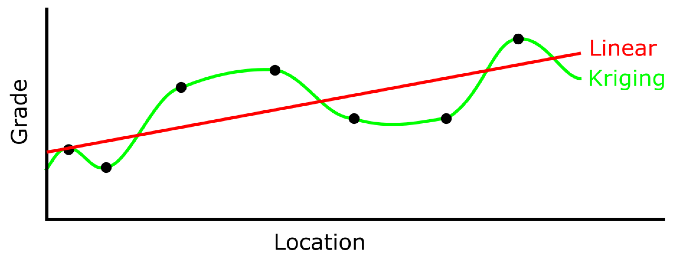
At this point, Matheron’s concept of a regionalized variable is invoked to calculate the best estimate that minimizes mean squared error. This estimate is sometimes called a linear estimate, but that is misleading in the current era of machine learning. Kriging is a locally linear estimator that leads to a highly non-linear response surface. The following sketch illustrates this in Figure 1; note how kriging leads to a complex, non-parametric, non-linear response surface. In machine learning, the red line would be considered a linear estimate. This does not imply that machine learning estimates are not valuable or that kriging is the ultimate local estimator. This author believes that a hybrid data-driven (ML) and model-driven (to some extent kriging) system would provide the best estimates. The author also believes that using focused AI models would greatly assist the modern geomodeler. ML/AI techniques will not replace geostatistical techniques, given the tailored focus on extrapolating a very small data sample and the emphasis on geological data integration, but ML/AI methods are clearly going to revolutionize geostatistics along with every other discipline.

Ordinary Kriging (OK) is the variant that has proven itself in hundreds of deposits (based on publicly disclosed resources). OK constrains the local estimates to be based only on the local data with no influence from the prior mean. The optimization of the kriging weights requires knowledge of the covariance between all pairs of data and all data and the unsampled location. These covariances come from a variogram model that is inferred from the data and from the judgement of the practitioner; therefore, it is a function that is both data-driven and model-driven.

There are alternative methodologies like multiple-indicator kriging and uniform conditioning that aim to get some probabilistic insight from inherently deterministic estimates. They have not seen wide application, yet they deserve mention.

These conventional deterministic techniques, specifically OK, are widely used. With careful parameter tuning, such as search restrictions, they can lead to resource estimates that are suitable for resource assessment and mine planning. There are, however, important limitations. The models do not show the same variability as the underlying true deposit; the histogram of estimates can easily be constrained to have the right variance, but the variogram of the estimates will always show that they have greater continuity than the true grades. The variability matters for decisions related to blending and other short-term grade-control decisions. The non-linearity of geometallurgical properties also entails that kriged estimates are potentially biased. Another limitation is that no reasonable assessment of uncertainty is provided.

3. Simulation and Probabilistic Techniques

Uncertainty in rock properties at unsampled locations is accepted. There is variability at all scales and relatively widely spaced drilling leads to inevitable uncertainty. Conventional geostatistical techniques have been extended to create numerical models that represent natural variability and quantify uncertainty.

Regarding multivariate and multilocation uncertainty, multivariate Gaussian (MG) distribution has unparalleled mathematical tractability and has seen widespread application. The MG distribution is fully parameterized by a mean vector and covariance values. Data are transformed into a Gaussian form, and then the required parameters are inferred from the data and from assumptions of stationarity. Local uncertainty is easily calculated and back-transformed into original units. There is no need for simulation to assess uncertainty in variables at the data scale; however, large-scale uncertainty for selective mining unit (SMU) blocks, stopes, pushbacks, dumps and tailing structures is required. Simulation is invoked to transfer uncertainty to a larger scale.

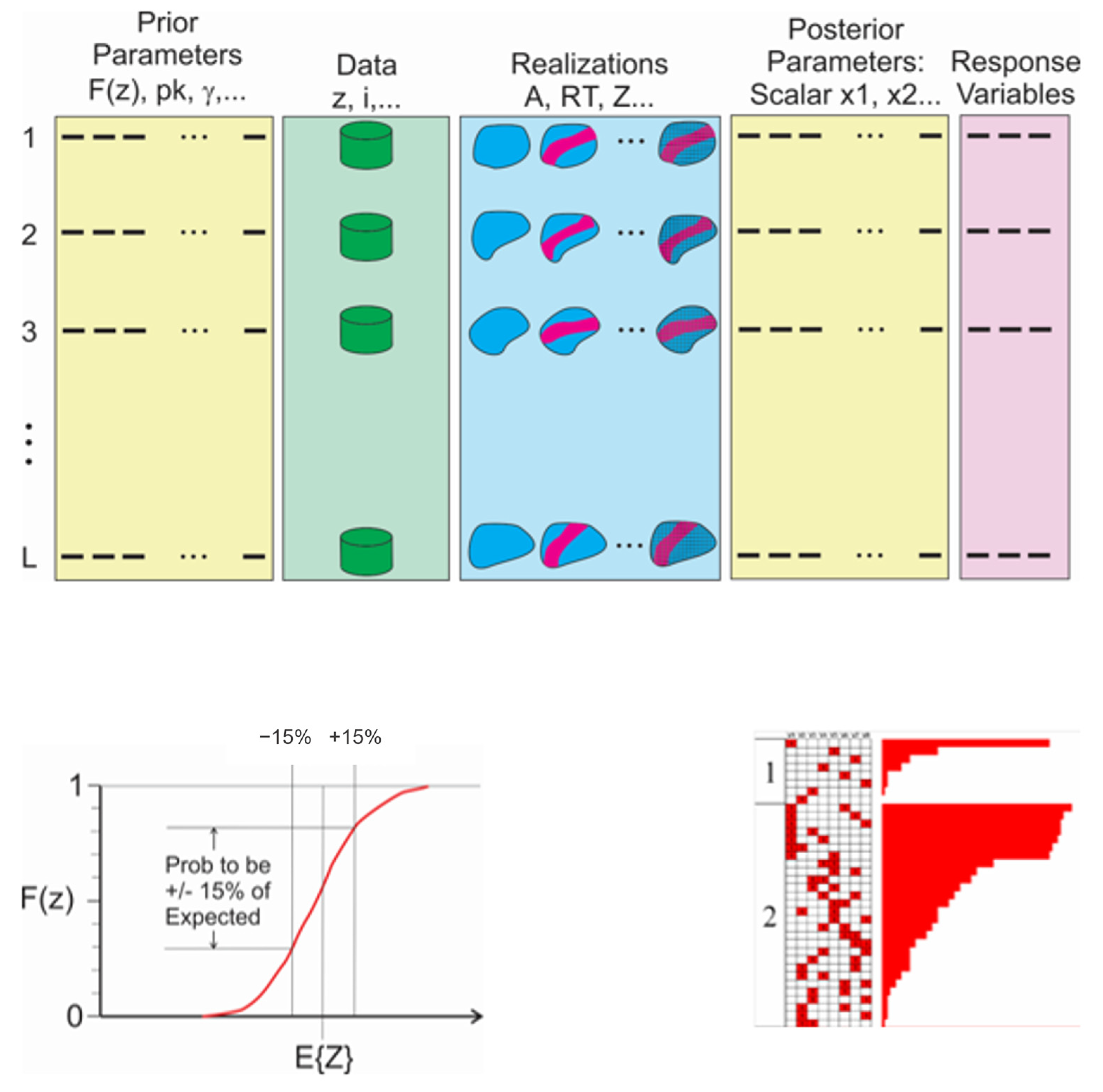
Simulation from a multilocation, multivariate (and perhaps multidata-type) MG distribution is not sufficient for practical large-scale uncertainty. Practice has shown that accurate and precise large-scale uncertainty requires capturing uncertainty in modeling parameters, the data used in modeling, large-scale domain boundaries, categorical variables and multiple continuous rock properties. A number of realizations would be yielded from each of the multiple scenarios. Figure 2 illustrates this in a schematic way.

Regarding Figure 2, there are many points being illustrated. Simulated realizations are illustrated in the top row, while post-processing is illustrated in the bottom row. Each of the L simulated realizations is one outcome of all required model characteristics: prior parameters that are needed to simulate the spatial models, the data that are used to locally condition the models, the hierarchical models of boundaries (A), the domains or rock types (RT) and the continuous rock properties (Z). The central blue panel represents The Geologic Model in a simulation context. It could be summarized through the use of posterior parameters such as volumes, proportions, mean values and correlation coefficients. Response variables of interest, such as tonnage, grade and metal estimates, are computed from each realization. The bottom row in Figure 2 illustrates the distribution of uncertainty in one particular response variable with an expected value (we get one number if we want one), and a representation of the sensitivity of the model characteristics to the posterior parameters is assessed. Managers would want to know the expected value, uncertainty and sensitivity; that is, the dependency of the uncertainty on different aspects of the geological model.

The approach illustrated schematically in Figure 2 is needed for large-scale resource/reserve uncertainty. In grade control, the required distributions and uncertainty are local and small-scale. In the design of blending facilities, variability is of primary importance, and the full hierarchical uncertainty may not need to be quantified. It is interesting to note that a simple, theoretically clean model of uncertainty from a Bayesian perspective is not practical. The prior model is a hybrid of many different variables and parameters. Updating by data is achieved in the process of simulation, but not with a clear equation. A review is now made on the application at different times in the life cycle of mineral deposits.

4. Application of Simulation and Probabilistic Techniques in Stages of Mining

The increased computational and professional time cost of simulations and probabilistic techniques are dwarfed relative to the improvements in data spacing, mitigation of risk and improved decision making. The application during the stages of the life cycle of mining are reviewed below. There is overlap. Optimizing drill hole spacing is an ongoing activity for different purposes. Quantifying the uncertainty of in situ resources is ongoing. Despite the overlap, there are some characteristic problems faced at different stages in the life cycle of a mineral deposit.

4.1. Prospecting

This stage is perhaps the least amenable for geostatistical techniques: (1) there may not be enough data to even know how much data are required; data collection would proceed in a staged fashion until some basic understanding is achieved; (2) related to the first point, there may be too few direct measurements to compute maps with any confidence; and (3) further emphasizing the lack of data, the underlying geological controls may be so uncertain that a statistical model cannot be formulated with any confidence. Nevertheless, there are situations when geostatistical tools have a place, specifically those situations with multiple data types.

Figure 3 shows a glimpse of some results that illustrate mapping over a large area. Geostatistical simulation techniques are applied to generate realizations of 39 primary variables conditioned to direct measurements and many (26) secondary variables. This is computed at a high resolution over a very large area. Computing the resources on many realizations provides uncertainty in resources at any scale. Of particular interest is local uncertainty: surely good is indicated by a high probability of good quality; surely bad is indicated by a high probability of low quality; average is indicated by a high probabilityof being within narrow bounds of the center of the distribution, and; highly uncertain is indicated by a simultaneous reasonable probability of being low and high.

Although there may be no drilling, there may be a significant number of geochemical, geophysical and other remote sensing data. An important task is to calibrate all of the available measurements for the prediction of pathfinder minerals or other indicators of potential targets using multivariate exploratory data analysis together with spatial mapping and reasoning.

Prospecting and exploration are associated with a strong opportunity-seeking position on risk. Short-term mine planning is risk-neutral—just take the best decision at the moment. Medium- and-long term mine planning is often risk-averse—avoiding the chance of underperformance and not meeting targets. Processing the multiple realizations generated in this situation would consider summaries aimed at the high quantiles of the distributions of uncertainty. A small probability of something significant is more interesting than a certain probability of some modest resource.

4.2. Exploration

Prospecting may not consider a geostatistical model with a quantified uncertainty and position on risk. There is a place for geostatistics, but the emphasis is on geological understanding and searching for a confluence of positive indicators. When that happens, acquisition of land rights and the appropriate permits to drill are acquired. The cost of this is significant enough to ensure the targets are chosen appropriately. The types of companies performing prospecting versus exploration and mining may be different. Exploration may start by acquiring a project that has passed the hurdle of success dictated by prospecting.

Regarding exploration, as in many life decisions, the goal is acquiring early negative information or early positive information—exit quickly or pursue aggressively. A minimum amount of information is required for this. A minimum amount of drilling is required considering the key question: how much data do we need to know how much data we need? This is subjective but also based on well-considered drill hole spacing studies. Early in the exploration, there will be few measured resources; mostly indicated and inferred resources will be delineated and disclosed. Geostatistical simulation will be considered to quantify the drill hole spacing required for classifying rock volumes as measured, indicated and inferred.

Some discussion on the requirements for classification is warranted. Clearly, the ultimate requirements are based on regulatory requirements that are passed down to professional organizations like CIM and AUSIMM. The judgement of qualified professionals together with procedures accepted by qualified peers are essential. Increasingly, professionals are considering classification based on geometric criteria aimed at (1) relevant production volumes, considering monthly, quarterly or annual production volumes, and (2) a statistical tolerance close to the predictions to those of the production volumes. For example, measured resources would require quarterly production volumes to be within 15% of the predicted with a 90% or greater probability. Indicated resources would require annual production volumes to be within 15% of the predicted with a 90% or greater probability. These conditions are not enshrined within reporting codes, but they are becoming a de facto standard. The only way to be confident in these probabilistic criteria (or similar site-specific criteria) is with the careful application of geostatistical simulation. Deterministic kriging calculations would not provide the required decision-support information.

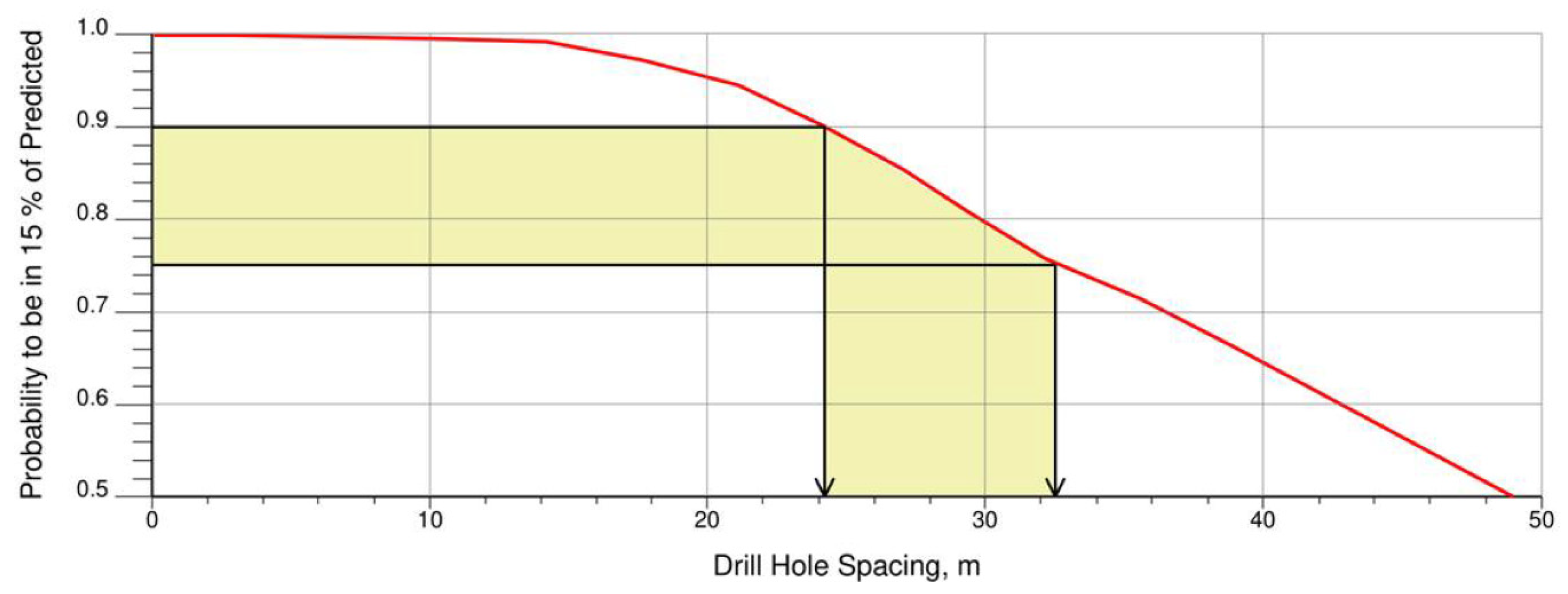
Figure 4 illustrates the results of a drill hole spacing study. The probability being within 15% of the predicted relates to the quantity of metal within a nominal quarterly production volume. The shaded range of uncertainty and drill hole spacing may be appropriate for classification. Note that 90% probability may be optimistic for a highly variable deposit type (precious metals) and pessimistic for a more continuous deposit type (coal, potash and industrial minerals). A range should be considered.

A key decision during exploration modeling is anticipation of the selectivity that would be attained during mining. Creating an over-smoothed model assuming no selectivity would be unrealistic. A highly selective model that is unattainable in future modeling would also be unrealistic. The models estimated during exploration should be generated for specific target mining methods. The information effect is important, that is, it acknowledges that the model constructed during exploration does not have access to the final information that will ultimately be available at the time of mining.

Increasingly, geostatistical models must consider data integration of mm-scale scanning data, different drilling types and large-scale remote sensing data. Simulation techniques are available to accommodate these different data types. More conventional deterministic techniques are limited in their ability to consider multiple data types.

Additionally, of increasing importance is the consideration of geometallurgical models that help forecast processing performance, such as recovery, energy consumption, reagent consumption, throughput rate and others. This is an important multivariate modeling problem that almost always includes a component of machine learning. Related to this is the importance of geomechanical models related to energy consumption, stability, support requirements and engineering design. Modern geostatistics is the modeling of whole-rock properties and not simply economic elements.

4.3. Development

The topics here transition between exploration and exploitation. Development is more strictly focused on construction, prestripping and establishing critical infrastructure before starting production. The details of mining, equipment selection and mining practices are optimized.

Although relatively few new drill holes will become available during development, the resource block model will be refined from the feasibility study block model. The appropriate selectivity and blending criteria will be confirmed, and the estimation plan of conventional block models are fine tuned to represent mine selectivity. In many cases, the additional data that become available are aimed at geometallurgical and geomechanical properties for engineering design. Refined multivariate modeling techniques may be considered for the improved modeling of these properties with many and varied data.

Simulation is also considered for a variety of reasons, including to (1) confirm drill hole spacing ahead of production, (2) mitigate the risk of underperformance, and (3) refine strategies and facilities for blending and homogenization. Figure 5 illustrates the results of a simulation study, establishing how uncertainty changes with scale. As the time period increases, the volume increases, and the uncertainty reduces. Processing facilities must be flexible enough to deal with this uncertainty, or additional data would be acquired.

Strategic mine planning under uncertainty is becoming more widely used. Geological uncertainty is quantified through the use of geostatistical methods, and then engineering design proceeds in a manner to mitigate the probability of undesirable outcomes and maximize the probability of desirable outcomes. An ability to quantify geological uncertainty is essential for this emerging field.

4.4. Exploitation

There are three main tasks for geological modeling during exploitation: (1) updating the life of mine (LOM) model with new drilling and improved geological understanding, (2) short-term or grade control models for choosing the correct destination for material during mining operations, and (3) characterizing waste rock structures, including tailings. There are many other minor tasks, including supporting nearby brown-field exploration, increasingly refined geometallurgical and geomechanical modeling and supporting decisions related to the adoption of new technology and mining methods.

Updating the life of the mine model follows the principles described above; however, short-term or grade control models are constructed differently. Those models are required weekly, if not daily, and are essential to the economic success of the mining project. The short-term model works in the context of a medium- and long-term model. Surface mining has different selectivity decisions and often mines more waste rock than underground mining. Geostatistical simulation supports optimal stope boundaries and stope sequencing in short-term planning of underground mining.

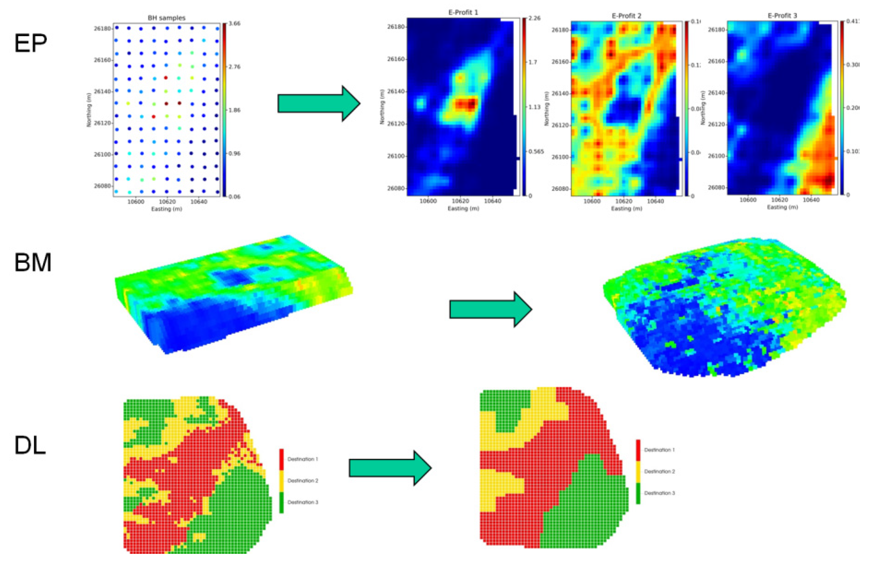
Regarding surface mining, Figure 6 illustrates the simulation applied to grade control. EP refers to calculating the expected profit for each high-resolution parcel of rock for each possible destination. BM refers to numerically modeling blast movement; that is, translating the high-resolution rock properties from the pre-blast geometry to the post-blast muckpile. DL refers to dig limits where practical mining shapes or polygons are determined. In simple cases, ore and waste are determined using a cutoff grade on one metal in the presence of constant recovery. In this case, the decision based on a cutoff grade applied to kriging and the maximum expected profit decision (the optimal one) is the same. Increasingly, however, there are non-linear effects due to variable recovery, multiple elements of value, non-linear influence of contaminants, etc. In the presence of these complexities, multivariate simulation should be considered, and an engineering/economic model should be applied to determine the optimal destination of each parcel of rock. The “parcels” should be high-resolution—about one-quarter of the data spacing—and then practical mining constraints should be considered. Mining contacts are unlikely to be aligned with the coordinate system or the pattern of blast holes; therefore, high-resolution modeling and posterior consideration of mining constraints are recommended (See Figure 7).

There are important references documenting the increased importance of grade control [16,17,18,19,20,21]. These document the importance of non-linearity, multivariate modeling, blast movement, and the use of simulation. Geostatistical simulation adds value to grade control by determining the optimal destination for mined material. Choosing the optimal destination based on the maximum expected profit is correct. The principle of “take the expected value as late as possible” is key in dealing with uncertainty. The expected value calculated from many realizations is not the value calculated on the expected grade. The main application of simulation in grade control is to transfer uncertainty in the presence of non-linear value calculations.

Medium-term models are also constructed during exploitation. These support intermediate-term tactical decisions and longer-term strategic decisions, such as reconsideration of pit stages, developing new areas, and tuning equipment choices.

As mining proceeds, waste rock structures such as dumps and tailings ponds grow and must be characterized for government reporting requirements, ongoing stability and safety, and engineering design and management. Data collected on the properties of waste rock structures are relatively sparse, and simulation provides an assessment of the consequent uncertainty and a means to manage the risk of non-performance.

4.5. Reclamation

The final stage in the lifecycle of a mining operation may be the most important. Restoring the disturbed land to a state as good as or better than originally encountered is central to the belief system of modern mining. This is a point of pride and not a burden or cost that is grudgingly encountered when revenue is no longer being generated. Progressive regulations will reinforce this and set boundaries that are mutually agreed upon by the legislators, miners and other stakeholders. Geostatistical simulation is used for a variety of activities during this last stage in the life cycle of a mineral deposit.

Waste rock structures, including dumps and tailing dam containments, must be monitored for stability and compliance with requirements of safety and the long-term planned outcome. There are questions to be answered through the use of simulations. A critical question is the optimal sample collection to use for acceptable uncertainty and reporting to the government and other stakeholders. At this point in the life cycle, the plan should be clear (certain or determined) with no room for non-compliance; however, sampling and ongoing monitoring are required to ensure that any deviation is acceptable. Geostatistical modeling, in particular, simulation, will establish an uncertainty band that will either lead to the acquisition of additional data or satisfy stakeholders of the efficacy of the planned containment.

Geostatistical simulation also supports many other geotechnical, erosion, subsidence, and fate/transport models. A key component is to ensure that outcomes are within regulated limits with high confidence.

5. Discussion

There are many quotes regarding the benefits of a poor understanding of uncertainty versus unwarranted confidence in a single estimate. Simulation and probabilistic techniques are partially aimed at uncertainty, but they are also aimed at understanding variability and passing input variables through complex non-linear transfer functions in an unbiased manner. The main aim of this paper has been to highlight the value and importance of simulation and probabilistic techniques through the life cycle of a mine.

6. Conclusions

The spatial distribution of rock properties in naturally occurring or engineered rock structures is uncertain due to heterogeneity and limited sampling. Simulation and probabilistic techniques are used to quantify this uncertainty and the risk of underperformance. These techniques are used to identify areas of opportunity, optimize the drill hole spacing during exploration and production, support risk-qualified mine planning, optimally route material to alternative destinations and manage waste structures during reclamation. The techniques for these tasks are available, but development is ongoing to manage a wide variety of data types, perform calculations quicker and in an automated fashion and promote the most precise and accurate uncertainty characterization.

References

- Krige, D.G. A statistical Approach to Some Mine Valuation and Allied Problems on the Witwatersrand. Master’s Thesis, University of the Witwatersrand, Johannesburg, South Africa, 1951. [Google Scholar]
- Matheron, G. Principles of geostatistics. Econ. Geol. 1963, 58, 1246–1266. [Google Scholar] [CrossRef]
- Matheron, G. The theory of regionalized variables and its applications. In Les Cahiers du Centre de Morphogie Mathématiqu de Fontainebleau, 5th ed; Ecole Nationale Superieure des Mines de Paris: Paris, France, 1971. [Google Scholar]
- David, M. Geostatistical Ore Reserve Estimation; Elsevier: Amsterdam, The Netherlands, 1977. [Google Scholar]
- Journel, A.G.; Huijbregts, C. Mining Geostatistics; Academic Press: London, UK, 1978. [Google Scholar]
- Isaaks, E.H.; Srivastava, R.M. An Introduction to Applied Geostatistics; Oxford University Press: New York, NY, USA, 1989. [Google Scholar]
- Deutsch, C.V.; Journel, A.G. GSLIB: Geostatistical Software Library: And User’s Guide, 2nd ed.; Oxford University Press: New York, NY, USA, 1998. [Google Scholar]
- Goovaerts, P. Geostatistics for Natural Resources Evaluation; Oxford University Press: New York, NY, USA, 1997. [Google Scholar]
- Sinclair, A.J.; Blackwell, G.H. Applied Mineral Inventory Estimation; Cambridge University Press: Cambridge, UK, 2002. [Google Scholar]
- Chiles, J.; Delfiner, P. Geostatistics: Modeling Spatial Uncertainty, 2nd ed.; John Wiley & Sons: Hoboken, NJ, USA, 2012. [Google Scholar]
- Pawlowsky-Glahn, V.; Olea, R.A. Geostatistical Analysis of Compositional Data; Oxford University Press: New York, NY, USA, 2004; 304p. [Google Scholar]
- Caers, J. Modeling Uncertainty in the Earth Sciences; John Wiley & Sons: Hoboken, NJ, USA, 2011. [Google Scholar]
- Pyrcz, M.; Deutsch, C.V. Geostatistical Reservoir Modeling, 2nd ed.; Oxford University Press: New York, NY, USA, 2014. [Google Scholar]
- Rossi, M.E.; Deutsch, C.V. Mineral Resource Estimation; Springer Science & Business Media: Dordrecht, The Netherlands, 2013. [Google Scholar]
- Azevedo, L.; Soares, A. Geostatistical Methods for Reservoir Geophysics; Springer International Publishing: New York, NY, USA, 2017. [Google Scholar]
- Verly, G. Grade control classification of ore and waste: A critical review of estimation and simulation based procedures. Math. Geol. 2005, 37, 451–475. [Google Scholar] [CrossRef]
- Barnett, R.M.; Manchuk, J.G.; Deutsch, C.V. The Projection-Pursuit Multivariate Transform for Improved Continuous Variable Modeling. SPE J. 2016, 21, 2010–2026. [Google Scholar] [CrossRef]
- Vasylchuk, Y.V.; Deutsch, C.V. Approximate blast movement modelling for improved grade control. Min. Technol. 2019, 128, 152–161. [Google Scholar] [CrossRef]
- Vasylchuk, Y.V.; Deutsch, C.V. Improved grade control in open pit mines. Min. Technol. 2017, 127, 84–91. [Google Scholar] [CrossRef]
- Boucher, A.; Dimitrakopoulos, R.; Vargas-Guzman, J.A. Joint Simulations, Optimal Drillhole Spacing and the Role of the Stockpile. In Geostatistics Banff; Leuangthong, O., Deutsch, C.V., Eds.; Springer: Berlin/Heidelberg, Germany, 2004; pp. 35–44. [Google Scholar]
- Dimitrakopoulos, R.; Godoy, M. Grade control based on economic ore/waste classification functions and stochastic simulations: Examples, comparisons and applications. Min. Technol. 2014, 123, 90–106. [Google Scholar] [CrossRef]
Figure 1.
The sketch illustrates that Kriging is a locally linear estimator, leading to a highly non-linear response surface.
Figure 2.
This figure illustrates the process for practical simulation and post-processing. The top row illustrates realizations in quantifying and transferring uncertainty. The bottom row summarizes post-processing. See the text below.
Figure 3.
A brief summary of a probabilistic study over a 170 by 300 km area in Northeast Alberta. Clockwise from the upper left: (1) a correlation matrix between 26 secondary variables from seismic surveys and mapping exercises and 39 primary variables related to thickness and quality—note that blue colors represent negative correlation, green is close to zero, and hotter colors represent more significant positive correlations, (2) a map showing data (over 16,000 were available from public records and a heat map of an expected primary variable, and (3) bar chart of bitumen in place for three different sub-areas with reasonable data.
Figure 4.
This figure illustrates how uncertainty increases (certainty decreases) as the drill hole spacing increases. The probability of being within 15% of the predicted relates to the quantity of metal within a nominal quarterly production volume. The shaded range of uncertainty and drill hole spacing may be appropriate for classification.
Figure 5.
An illustration of how uncertainty changes with scale. As the time period increases, the volume also increases. There is more averaging within large volumes, and the uncertainty reduces.
Figure 6.
This figure illustrates the simulation applied to grade control. EP refers to calculating the expected profit for each high-resolution parcel of rock for each possible destination. BM refers to numerically modeling blast movement—translating the high-resolution rock properties from the pre-blast geometry to the post-blast muckpile. DL refers to dig limits where practical mining shapes or polygons are determined.
Figure 7.
This figure illustrates that a resolution of between 20 to 30 percent of the data spacing is reasonable to resolve contacts that are not aligned with the data or the coordinate system. The red line represents the true underlying ore/waste contact (ore to the left and waste to the right). A coarse grid block network would not follow that line very precisely. A resolution of less than 20% of the data spacing is not justified by the available data.
Disclaimer/Publisher’s Note: The statements, opinions and data contained in all publications are solely those of the individual author(s) and contributor(s) and not of MDPI and/or the editor(s). MDPI and/or the editor(s) disclaim responsibility for any injury to people or property resulting from any ideas, methods, instructions or products referred to in the content. |
© 2023 by the author. Licensee MDPI, Basel, Switzerland. This article is an open access article distributed under the terms and conditions of the Creative Commons Attribution (CC BY) license (https://creativecommons.org/licenses/by/4.0/).
Share and Cite
MDPI and ACS Style
Deutsch, C.V. The Place of Geostatistical Simulation through the Life Cycle of a Mineral Deposit. Minerals 2023, 13, 1400. https://doi.org/10.3390/min13111400
AMA Style
Deutsch CV. The Place of Geostatistical Simulation through the Life Cycle of a Mineral Deposit. Minerals. 2023; 13(11):1400. https://doi.org/10.3390/min13111400
Chicago/Turabian StyleDeutsch, Clayton V. 2023. "The Place of Geostatistical Simulation through the Life Cycle of a Mineral Deposit" Minerals 13, no. 11: 1400. https://doi.org/10.3390/min13111400
Note that from the first issue of 2016, this journal uses article numbers instead of page numbers. See further details here.