Integrated Stochastic Underground Mine Planning with Long-Term Stockpiling: Method and Impacts of Using High-Order Sequential Simulations

Abstract

The integrated optimization of stope design and underground mine production scheduling is an approach that has been shown to effectively leverage the synergies among these two underground mine planning components to generate truly optimal stope layouts and extraction sequences. The existing stochastic integrated methods, however, do not include several elements of a mining complex, such as stockpiles, due to the computational complexity and non-linearity that they might add to the optimization of the long-term mine plan. Additionally, sequential simulation methods that rely on two-point statistics and Gaussian distribution assumptions are commonly used to generate the input realizations of the mineral deposit. These methods, however, are not able to properly characterize complex spatial geometries or the high-grade connectivity of non-Gaussian and non-linear natural phenomena. The present work proposes an extension of previous developments on the integrated stope design and underground mine scheduling optimization through an expanded stochastic integer programming formulation that incorporates long-term stockpiling decisions. An application of the proposed method at an operating underground copper mine compares the cases in which the geological simulated orebody models are based on high-order and Gaussian sequential simulation methods. The extraction sequence and related final stope design are shown to be physically different. It is seen that the optimization process takes advantage of the better representation of high-grade connectivity when high-order sequential simulations are used, by targeting the areas with grades that follow the mill’s blending requirements and by making less use of the stockpiles. Overall, a 4% higher copper metal production and a resultant 6% higher net present value are observed when high-order sequential simulations are used.

1. Introduction

Sublevel longhole open stoping (SLOS) is an underground mining method in which the orebody is divided into vertically oriented open stopes that are self-supported by rock pillars and are posteriorly backfilled. Horizontal extraction levels define the vertical boundaries of the stopes, and sublevel drifts and crosscuts are developed to enable longhole drilling [1,2,3]. The long-term mine planning process for this mining method relies on three main components. The stope layout defines the spatial design of mineable volumes according to geomechanical and geological properties [4,5,6,7,8,9]. A network design of ramps, shafts, raises, wises, and other developments is completed in order to define accesses and ventilation systems [10,11,12]. The last component defines the production schedule of stopes by maximizing the net present value (NPV) of the related life-of-mine (LOM) [13,14,15,16,17,18,19,20,21,22,23]. Little et al. [17] show that these three components should be optimized simultaneously so that the interdependencies among stope grades, development costs, and the time value of money are captured in the mine planning optimization. In addition, geological uncertainty in grades and material types is known as a critical source of risk for mining projects and its management is essential for meeting production targets and generating realistic forecasts [24,25,26].

A mixed integer programming (MIP) model that integrates underground mine design and production scheduling was first proposed by Little et al. [17] and Little et al. [27]. The MIP maximizes the discounted cash flow of the mined stopes and considers the stope size and location, while under the constraints of the ore production and backfilling capacities. Therefore, the stope boundaries are an outcome of the production schedule. However, the costs associated with the development of access are not covered in this approach. Copland and Nehring [28] incorporate level access development decisions in an integer program (IP) that maximizes the discounted revenue from mined stopes while minimizing the level’s development costs. Foroughi et al. [29] optimize the underground mine production scheduling and stope layout through an IP that aims to jointly maximize two weighted objectives, the NPV and the overall metal recovery. Hou et al. [30] integrate the mathematical formulation into the development of longitudinal drives and shaft-level segments as unitary decisions linked to the stope’s extraction decisions. Although an analysis of the forecasts given different simulations of the orebody is conducted, the risk associated with the geological uncertainty is not managed or assessed through this approach. Furtado e Faria et al. [31] propose an integrated stochastic framework for the stope design and long-term mine production scheduling, tailored for the sublevel open stopping (SLOS) mining method. The authors develop a two-stage stochastic integer programming (SIP) [32] formulation that jointly optimizes the stope design and production scheduling while considering the cumulative development costs and managing the geological risk. Carelos Andrade et al. [33] also explore the integrated stochastic approach to the SLOS mining method variant that uses backfilling practices and adjacency patterns of primary, secondary, and tertiary stopes [34,35]. This optimization framework aims to maximize the NPV while managing the geological risk, by minimizing deviations from production targets, which are related to mining and processing capacities, as well as the grade blending requirements. An application at an operating copper mine with secondary elements shows significant improvement in terms of the NPV when compared to a stochastic sequential framework [33]. Nonetheless, an important aspect that has not been addressed in these models is the presence of stockpiles, which are typically used in mining operations. It has been shown that, for long-term open-pit mine planning and production scheduling, the consideration of all components of a mining complex in the optimization process leads to more realistic assumptions and forecasts [36,37,38].

In order to assess and manage the spatial uncertainty and variability of grades and material types, a set of geostatistical simulations of the orebody is used as the main input to the optimization of the stope design and production scheduling [26,30,31,39,40,41,42,43]. Geological attributes, such as metal grades and material types, can be modeled through geostatistical simulation methods that build upon the concept of spatial random fields [44,45,46,47,48,49]. The sequential simulation paradigm allows for the assessment of an attribute at an unsampled location, by its conditioning value to sample data and previously simulated values, via Monte Carlo sampling of a probability distribution function [44]. As an example, the sequential Gaussian simulation (SGS) [44,50] can be mentioned as a simulation method that is conventionally employed. The SGS method, however, does not reproduce the connectivity of high grades given that the Gaussian random function model has the character of maximum entropy [51]. In addition, this traditional method relies on two-point spatial statistics. Although second-order statistics can fully characterize Gaussian random functions, they do not describe complex geological patterns in the presence of non-Gaussianity and non-linearity [52,53,54,55].

Methods based on multiple-point statistics (MPS) are introduced to overcome the limitations of the aforementioned traditional simulation methods [49,53,54,55,56,57,58,59]. These methods infer the conditional probability distribution function (cpdf) by extracting multiple point patterns from a training image (TI) or geological analog, without making any assumptions about it. These MPS-based simulation approaches tend to reproduce the spatial statistics of the TI, while a consistent mathematical modeling approach should be driven by the sample data [60]. Dimitrakopoulos et al. [52] introduce the use of high-order cumulants to explicitly infer high-order statistics from the spatial data. Thus, the high-order simulation (HOSIM) algorithm follows the sequential simulation framework and uses spatial cumulants to derive the cpdf from available data, generating realizations that show the natural connectivity of high grades and reproduce complex geometries [61,62,63,64].

The impact of using different simulation algorithms to generate the mineral deposit models used as inputs for stochastic mine planning in open-pit mines has been studied by de Carvalho and Dimitrakopoulos [65]. The related work compares the long-term open-pit mine production schedules and forecasts when SGS and HOSIM [63] are used to generate the simulated orebody models serving as inputs to a simultaneous stochastic optimization framework [38,66,67,68]. The application shows that the long-term sequence of extraction of mining blocks favors the high-grade continuity areas when simulations generated using the HOSIM method are used. The comparison also shows different final pit limits. In addition, more gold is produced at the end of the life-of-mine (LOM), leading to a higher expected NPV, when the optimization uses simulations generated with the HOSIM method. Thus, it is of interest to investigate how a HOSIM approach impacts the stochastic stope design and mine production schedule, particularly given that underground mining methods make assumptions in terms of the ore selectivity and spatial configuration of mineable volumes.

The current work presents the extension of the integrated stochastic optimization of stope design and mine production scheduling proposed by Carelos Andrade et al. [33] by adding long-term stockpiling and related material destination decisions to the previously proposed SIP formulation. In addition, the sensitivity of the proposed scheduling model to different methods used for the geostatistical simulations of the mineral deposit involved is investigated in a case study at an operating underground copper mine. The case study presents the practical aspects of the proposed mathematical programming model based on simulated realizations of the copper deposit generated using a high-order sequential simulation approach [61]. In addition, the extraction sequence and forecasts are compared to those obtained when the deposit realizations are generated using sequential Gaussian simulation. The following section presents a description of the underground mine planning approach with the integration of a linear stockpile. A brief review of the sequential simulation methods, as relevant to the present study, is presented. Subsequently, a case study at an operating copper mine is presented, followed by conclusions and suggested future work.

2. Methodology

The following subsection presents an extended stochastic integer programming (SIP) formulation, which incorporates long-term stockpiling decisions into the integrated stochastic optimization of stope design and mine production scheduling, is presented. The method builds upon the work [33], on the optimization framework considering the sublevel longhole open stoping (SLOS) mining method with backfilling. The two stochastic simulation approaches [44,61] used in the case study to generate orebody models quantifying geological uncertainty, which are inputs to the optimization process are also summarized.

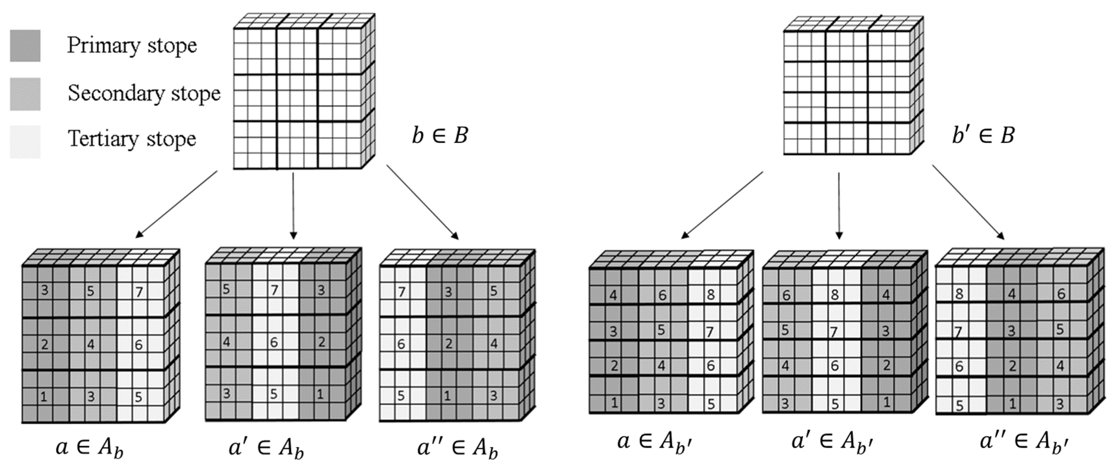
2.1. Mathematical Formulation of the Stochastic Long-Term Underground Mine Production Scheduling with Stockpiling

An extended stochastic integer program (SIP) [32] that incorporates long-term stockpiling decisions into the integrated stochastic optimization of stope design and mine production scheduling is proposed herein. The proposed method follows the optimization framework presented by Carelos Andrade et al. [33] for the sublevel longhole open stoping (SLOS) mining method with backfilling, as per an operating copper mine. Therefore, only the new aspects of this methodology are detailed herein. The method aims to optimize jointly the extraction sequence of stopes $j\in J$ and horizontal development costs of drifts $d\in D_l$ and crosscuts $c\in C_l$ that will lead to stope boundaries that respect the stopes’ geometric parameters. The approach assumes the optimization of a mining zone of a large orebody that defines a volume with unique geotechnical requirements. A set of geostatistical simulations $s\in S$ of the orebody describes the geological uncertainty. Initially, the orebody is represented in terms of blocks $i\in I$ that are, subsequently, grouped into stopes $j\in J$.

Three data processing steps are needed to generate the inputs necessary to the proposed two-stage SIP as shown in Figure 1, and summarized as follows. The first preprocessing step generates different mining zone configurations $b\in B$ by dividing the mining zone into different mining fronts and sublevels $l\in L$ according to allowable stope and sublevel dimensions; that is, shapes that reflect operational and geotechnical parameters. Crosscuts c are developed within each mining front, parallel to a defined mining direction. Drifts d are developed perpendicularly to the cross-cuts. The approximated dimensions of crosscuts ${\delta }_{j,c,l,b}^C$ and drifts ${\delta }_{j,d,l,b}^D$, as well as the length ${\delta }_{h,l,b}^V$ from the surface to the access point of a haulage system h and its respective mining zone configurations ${b\in B}_h$, for each sublevel $l\in L_b$. In the second preprocessing step, shown in Figure 1, for each configuration b, stope type options $a\in A_b$ are generated. Each stope type option $a$ defines a possible ordering of primary, secondary, and tertiary stope types $k\in K$, as exemplified in Figure 2. Each stope is identified by an indicator parameter ${\pi }_{k,j,b,a}$, according to its type. Therefore, the set of predecessors $\phi \in {\Phi }_{j,a}$ of a stope $j\in J_{j,a}$ can be defined following geotechnical constraints. Along these steps, the stopes are assumed to fully occupy the space between the sublevels. To manage dilution, in the third step, the profitability of having stopes with heights ${\mathsf{\gamma }}^{\mathrm{z}}$ that are smaller than the distance between sublevels and greater than the minimum stope height is evaluated. Thus, for a given mining zone configuration b, a stope type option a, a stope j, and elements $\epsilon \in E,$ the economic value of each stope $v_{j,b,a,s}\left({\mathsf{\gamma }}^{\mathrm{z}}\right)$ is calculated, as shown in Equation (1), for all its possible vertical dimensions ${\mathsf{\gamma }}^{\mathrm{z}}$ and for each simulated orebody scenario s. A probability of non-exceedance threshold (e.g., P50) is predefined, and only the economic value that corresponds to that threshold ($\mathrm{e}.\mathrm{g}.,v_{j,b,a}^{\mathcal{P}50}\left({\mathsf{\gamma }}^{\mathrm{z}}\right))$ is analyzed. The final stope heights are those that maximize the probabilistic economic value of a stope ($v_{j,b,a}^{\mathcal{P}}\left({\mathsf{\gamma }}^{\mathrm{z}}\right))$, as in Equation (2), as follows:

$$\begin{array}{c}{v}_{j,b,a,s}\left({\mathsf{\gamma }}^{\mathrm{z}}\right)=w_{j,b,s}\left({\mathsf{\gamma }}^{\mathrm{z}}\right)\left({\displaystyle \sum _{\epsilon \in E}}{g}_{j,b,\epsilon ,s}\left({\mathsf{\gamma }}^{\mathrm{z}}\right)R_{\epsilon }{P}_{\epsilon }-\left(C^P+{\displaystyle \sum _{k\in K}}{\pi }_{k,j,b,a}{C_k^{}}^M\right)\right), \\ \forall j\in J_b, b\in B, a\in A, s\in S\end{array}$$

(1)

$$\underset{{\mathsf{\gamma }}^{\mathrm{z}}}{\mathrm{argmax}}\begin{array}{c}{v}_{j,ba,}^{\mathcal{P}}\left({\mathsf{\gamma }}^{\mathrm{z}}\right)\\ \end{array},\forall j\in J_b,b\in B,a\in A$$

(2)

where $w_{j,b,s}\left({\mathsf{\gamma }}^{\mathrm{z}}\right)$ and $g_{j,b,\epsilon ,s}\left({\mathsf{\gamma }}^{\mathrm{z}}\right)$ are, respectively, the tonnage and grade of element ε within stope j in mining zone b, in scenario s, as a function of the stope height ${\mathsf{\gamma }}^{\mathrm{z}}$, $R_{\epsilon }$ is the metal recovery of element ε and $P_{\epsilon }$ is the related metal price, $C^P$ is the unitary processing cost and ${C_k^{}}^M$ is the unitary mining cost for each stope type. The function argmax, in Equation (2), returns the value of a stope height (${\mathsf{\gamma }}^{\mathrm{z}}$) that maximizes the probabilistic economic value of a stope ($v_{j,b,a}^{\mathcal{P}}\left({\mathsf{\gamma }}^{\mathrm{z}}\right))$.

Finally, the information generated in the three steps described above is used as input to the proposed extended two-stage SIP, that defines the fourth step of the presented method. The new SIP addresses the stope design and long-term production scheduling with the complement of stockpiling decisions. The related decision variables, objective function, and main constraints are described next. The mining zone configuration decision variables $z_{b,a}\in \left\{\mathrm{0,1}\right\}$ control which mining zone configuration $b\in B$ and respective stope type option is selected $a\in A_b$. These decision variables directly impact the selections of stope shapes and types. A mining zone is associated with one or more haulage systems $h\in H$. Therefore, identical mining zone configuration options ($b$ and b′), in terms of stope shapes and sublevels, can exist but they will be associated with different available haulage systems ($b\in B_h,$ and $b^{\prime }\in B_{h^{\prime }})$. It is assumed that vertical accesses compatible with the haulage systems are already developed, which enables the variable $z_{b,a}$ to be time-independent. The stope selection decision variables $y_{j,b,a,t}\in \left\{\mathrm{0,1}\right\}$ determine if a stope $j\in J_b$ in a mining zone configuration $b\in B$, using stope type option $a\in A_b$ is mined in period $t\in T$ and sent directly to the processor. A variable $x_{j,b,a,t,t^{\prime }}\in \left\{\mathrm{0,1}\right\}$ controls the extraction sequence and posterior reclamation of stockpiled stopes by defining if a stope $j\in J_b$ in a mining zone configuration $b\in B$, using stope type option $a\in A_b$ is mined and sent to a stockpile in period t and rehandled at period $t^{\prime }>t$. Thus, it is assumed that a stockpile for each time period $t^{\prime }$ can exist, or that the selection of the material of stopes within a stockpile is possible, in order to have a linear formulation [69].

Two continuous decision variables ${\psi }_{d,l,b,t }$ and ${\psi }_{c,l,b,t}$ correspond to the developed distance of a drift d or a cross-cut c, for a sublevel l, in a mining zone configuration b, in period t. To account for the available structures developed in previous years, effective development distances ${\psi }_{d,l,b,t}^{*}$ and ${\psi }_{c,l,b,t}^{*}$ are used in practice and they correspond to the cumulative horizontal development distances. The remaining decision variables refer to surplus deviations from haulage capacities for different haulage systems h$\left(d_{h,t,s}^H\right)$, processing capacity ($d_{p,t,s}^P$) and stockpiling capacities ($d_{t,s}^S$), and deviations from lower and upper bounds for different elements $\epsilon \in E$ requirements, ${d_{\epsilon ts}}^{-}$ and ${d_{\epsilon ts}}^{+}$, respectively. Additional technical and economical parameters are presented in

Table 1. List of technical and economic parameters.

Index	Definition
$w_{j,b,s}$	Tonnage of stope j, in mining zone configuration b, stope sequencing option a, and in geological scenario s
$g_{j,b,\epsilon ,s}$	Grade of element ε within stope j in mining zone b, in scenario s
$f_t^{EDR}$	Economic discount factor for period t given an economic discount rate
$C_{l,t}^H$	Discounted horizontal development discounted cost in sublevel l, at period t in $/km
${C_{k,t}^{}}^M$	Discounted mining cost for type k stopes at period t in $/t
$C^P$	Unitary processing cost $/t
$C_t^R$	Discounted rehandling cost at period t in $/t
$C_{h,b,t}^H$	Discounted haulage cost at period t if $h\in H_{ramp}$ in $/(tons×km) and if $\in H_{shaft}$ in $/t
$F_{bt}$	Fixed discounted cost for keeping the mining zone configuration b
$U_t^S$	Stockpiling capacity at period t (tons/year).

.

Once stockpiling decisions are considered, mining, rehandling, and processing costs can be incurred in different periods for a given stope. Therefore, Equation (3) describes the general profit of a stope at the period during which this stope is processed.

$$p_{j,b,a,s,t}={f_t^{EDR}w}_{j,b,s}\left(\sum _{\epsilon \in E}{g}_{j,b,\epsilon ,s}{R}_{\epsilon }{P}_{\epsilon }-C^P\right),\forall j\in J_b,b\in B,a\in A,s\in S$$

(3)

Equation (4) presents the objective function in five parts. Part I aims to maximize the discounted revenue from the stopes that are mined and processed at the same period. Part II maximizes the revenue from the scheduled stopes that are stockpiled by applying the discounted mining and rehandling costs according to the year in which they are incurred in the production schedule. Haulage costs are managed in different ways depending on the transportation systems available and chosen by the optimizer. If material is hauled through a ramp, the distance from the sublevel to the surface (${\delta }_{h,b,l})$ must be considered; otherwise, if the material is hauled through a skip, the parameter ${\delta }_{h,b,l}$ is set as one. Part III of the objective function minimizes the effective development costs and part IV minimizes a fixed cost for keeping the mining zone in operation. Finally, part V manages the geological risk by minimizing the deviations from the production targets related to mining, stockpiling, and processing capacities as well as grade blending requirements. For that purpose, penalty costs $c_h^H,c^P,c^S{c}_{\epsilon }^{+} \mathrm{a}\mathrm{n}\mathrm{d} c_{\epsilon }^{-}$ are applied to correspond to the production requirements and targets, as they are discounted by a geological risk discounting factor $f_t^{GRD}$ [70].

$$\begin{gathered} \mathit{max}\frac{1}{\left|S\right|}\underset{PartI}{\underbrace{\sum _{s\in S}\sum _{t\in T}\sum _{b\in B}\sum _{a\in A_b}\sum _{j\in J_b}\left(p_{j,b,a,s,t}-w_{j,b,s}\left(\sum _{k\in K}{\pi }_{k,j,b,a}{C}_{kt}^M-\sum _{h\in H}{\displaystyle \sum _{l\in L_b}}{\delta }_{h,b,l} C_{h,b,t}^H\right)\right)y_{jbat}}} \\ +\underset{PartII}{\underbrace{\frac{1}{\left|S\right|}\sum _{s\in S}\sum _t^{\left|T-1\right|}\sum _{t^{\prime }=t+1}^{\left|T\right|}\sum _{b\in B}\sum _{a\in A_b}\sum _{j\in J_b}\left(p_{j,b,a,s,t^{\prime }}-w_{j,b,s}\left(\sum _{k\in K}{\pi }_{k,j,b,a} C_{k,t}^M-\sum _{h\in H}{\displaystyle \sum _{l\in L_b}}{\delta }_{h,b,l} C_{h,b,t}^H-C_{t^{\prime }}^R\right)\right)x_{j,b,a,t{,t}^{\prime }}}} \\ -\underset{PartIII}{\underbrace{\sum _{t\in T}\sum _{b\in B}\sum _{l\in L_b}{C}_{l,t}^H\left(\sum _{d\in D_l}{\psi }_{d,l,b,t}^{*}+\sum _{c\in C_l}{\psi }_{c,l,b,t}^{*}\right)}} \\ -\underset{PartIV}{\underbrace{\sum _{t\in T}\sum _{b\in B}\sum _{a\in A_b}{F}_{bt}{z}_{b,a}}} \\ \underset{PartV}{\underbrace{\frac{1}{\left|S\right|}\sum _{s\in S}\sum _{t\in T}{f}_t^{GRD}\left(c_h^H{d}_{h,t,s}^H+c^P{d}_{t,s}^P+c^S{d}_{t,s}^S\sum _{\epsilon \in E}{c_{\epsilon }^{+}{d}_{\epsilon ,t,s}}^{+}+c_{\epsilon }^{-}{d_{\epsilon ,t,s}}^{-}\right)}} \end{gathered}$$

(4)

The objective function is subjected to reserve, adjacency, non-overlapping, and capacity constraints. The addition of decision variables that control both the extraction sequence and the stockpiling decisions requires a simple adaptation of the reserve, adjacency, and capacity constraints proposed by Carelos Andrade et al. [33]. New constraints are included to control the stockpiling capacity.

$${\sigma }_{t,s}=\sum _{b\in B}\sum _{a\in A_b}\sum _{j\in J_b}\left(w_{j,b,s}\sum _{t^{\prime }=2}^{\left|T\right|}{x}_{j,b,a,t,t^{\prime }}\right) \forall t=1,s\in S$$

(5)

$${\sigma }_{t,s}=\sum _{b\in B}\sum _{a\in A_b}\sum _{j\in J_b}\left(w_{jbs}\left(\sum _{t^{\prime }>t}^{\left|T\right|}{x}_{j,b,a,t,t^{\prime }}-\sum _{t^{\prime }=1}^{\left|T\right|}{x}_{j,b,a,t^{\prime },t}\right)\right)+{\sigma }_{t-1,s},\hspace{1em}\forall t>1,s\in S$$

(6)

$${\sigma }_{t,s}-d_{t,s}^S\le U_t^S,\hspace{1em}\forall t\in T,s\in S$$

(7)

Equations (5) and (6) calculate the value of an auxiliary variable ${\sigma }_{t,s}$ that defines the tonnage left at the stockpiles at the end of period t for scenario s. This tonnage is constrained by a maximum yearly capacity $U_t^{sp}$ that can be left stockpiled at the end of each period t, as shown in Equation (7).

2.2. Mineral Deposit Modeling Using Sequential Simulations

Consider $Z\left(u_i\right)$ a stationary ergodic random field indexed in $R^n$, where $u_i$, represents the location of the points $i=1\dots N$ of the grid to be simulated in a domain $D\subseteq R^n$. The set $d_n=\left\{z\left(u_{\mathsf{\alpha }}\right),\alpha =1\dots n\right\}$ denotes the original sample data conventionally obtained by the exploration data. A set ${\Lambda }_i$ represents the conditioning data for each node index by i. Therefore, ${\Lambda }_0=\left\{d_n\right\}$ is the conditioning data when the first point is simulated and only sample data is available and ${\Lambda }_i=\left\{{\Lambda }_{i-1}\cup Z\left(u_i\right)\right\}$ is the conditioning data for the subsequent points being simulated that includes the original sample data and previously simulated points. Accordingly, the sequential simulation paradigm defines that the joint probability density function (pdf) of the random field $Z\left(u_i\right)$ can be decomposed into the product of conditional univariate distributions [44,50].

$$f\left(u_1,\dots ,u_N;z_1,\dots ,z_N|d_n\right)=f\left(u_1,z_1|d_n\right)\prod _{i=2}^{N}f\left(u_i,z_i|{\Lambda }_{i-1}\right).$$

(8)

The conditional probability distribution function (cpdf) for any node $u_i$ can be written according to the Bayes’ rule as

$$f\left(u_i;z_i|{\Lambda }_0,{\Lambda }_{i-1}\right)=\frac{f\left({u_i;{\lambda }_0,{\lambda }_{i-1};z_0,\Lambda }_0,{\Lambda }_{i-1}\right)}{\int f\left({u_i;{\lambda }_0,{\lambda }_{i-1};z_0,\Lambda }_0,{\Lambda }_{i-1}\right)d{u}_i},$$

(9)

where ${\lambda }_0$ and ${\lambda }_{i-1}$ are the locations of the points in the conditioning data sets ${\Lambda }_0$ and ${\Lambda }_{i-1}$, respectively, and $f\left({u_{\mathit{i}};{\lambda }_0,{\lambda }_{i-1};z_0,\Lambda }_0,{\Lambda }_{i-1}\right)$ is the joint pdf.

2.2.1. High-Order Simulation Using Legendre-like Orthogonal Splines

To generate geostatistical simulations accounting for high-order spatial statistics [52,61,64], the method proposed by Minniakhmetov et al. [61], where the joint cpdf is approximated using high-dimensional polynomials combined with high-order spatial cumulants is used herein and summarized below.

$$\begin{array}{c}f\left({u_i;{\lambda }_0,{\lambda }_{i-1};z_0,\Lambda }_0,{\Lambda }_{i-1}\right)=\\ {\displaystyle \sum _{m_0=0}^{{\omega }_0}}{\displaystyle \sum _{m_1=0}^{{\omega }_1}}\dots {\displaystyle \sum _{m_n=0}^{{\omega }_n}}{L}_{m_0,m_1\dots m_n}{\phi }_{m_0}\left(z_0\right){\phi }_{m_1}\left(z_1\right)\dots {\phi }_{m_n}\left(z_n\right) ,\end{array}$$

(10)

where $L_{k_0,k_1,\dots k_n}$ are coefficients of approximation and ${\phi }_{m_0}\left(z_0\right){\phi }_{m_1}\left(z_1\right)\dots {\phi }_{m_n}\left(z_n\right)$ follows the orthogonality property as

$${\int }_a^b{\phi }_m{\phi }_k\left(z\right)dz={\delta }_{mk},$$

(11)

where ${\delta }_{m_n{k}_n}=\left\{\begin{array}{c}1,m=k\\ 0,m\ne k\end{array}\right.,\forall k=0\dots \omega$ is the Kronecker delta.

The orthogonal functions considered herein are Legendre-like orthogonal splines [61] and the Legendre coefficients $L_{k_0,k_1,\dots k_n}$ can be approximated experimentally by calculating

$$\begin{array}{c}{L}_{k_0,k_1,\dots k_n}\approx E\left[{\phi }_{k_0}\left(z_0\right){\phi }_{k_1}\left(z_1\right)\dots {\phi }_{k_n}\left(z_n\right)\right]\approx \\ \frac{1}{N_{h_1,h_2\dots h_n}}{\displaystyle \sum _{k=1}^{N_{h_1,h_2\dots h_n}}}{\phi }_{k_0}\left(z_0^k\right){\phi }_{k_1}\left(z_1^k\right)\dots {\phi }_{k_n}\left(z_n^k\right),\end{array}$$

(12)

where $z_i^k,i=0\dots n$ are values taken from a training image (TI), or geologic analog, that contains densely sampled geological information and represents complex geological structures.

The method relies on the definition of a spatial template formed by the central node being simulated and neighboring values separated by lag vectors $h_i=u_i-u_0,i=1\dots n$, which are used to scan the TI, to calculate the Legendre coefficients. The high-order sequential simulation algorithm follows:

• Define a random path for visiting all unsampled nodes on the simulation grid.
• For each node $u_0$ in the path:
  • Find the closest neighbor nodes $u_{1,}{u}_2,\dots u_n$.
  • Obtain the spatial template configuration by calculating the lag vectors $h_i$.
  • Scan the TI and find values $z_i^k,i=0\dots n$ given the spatial template configuration.
  • Calculate the spatial Legendre coefficients $L_{k_0,k_1,\dots k_n}$ using Equation (5).
  • Build the cpdf $f\left(u_i;z_i|{\Lambda }_0,{\Lambda }_{i-1}\right)$ by calculating the joint probability density function as in Equation (3) and normalizing it as shown in Equation (2).
  • Draw a uniform random value in [0, 1] to sample $z_0$ from the cumulative cpdf derived on the previous step.
  • Add $z_0$ to the set of conditioning data ${\Lambda }_i$ and move to the next node.
• Repeat steps 1 and 2 to generate different realizations.

2.2.2. Sequential Gaussian Simulation

The case study presented in Section 3 also uses sequential Gaussian simulation (SGS) [44,50,71] as an input, so that the related schedules and the forecast are compared to the ones obtained when the HOSIM is used. The method follows the sequential simulation paradigm while assuming a Gaussian conditional probability distribution function (cpdf) $f\left(u_I;z_i|{\Lambda }_0,{\Lambda }_{i-1}\right)$ that can be parametrized by its mean and variance. Initially, the original sample data is transformed to the Gaussian space, the experimental variogram is calculated from the transformed data, and the variogram model is inferred. Then, at each node, the Kriging system is used to obtain the conditional mean and variance, allowing the definition of a normal cpdf from which the simulated values will be sampled.

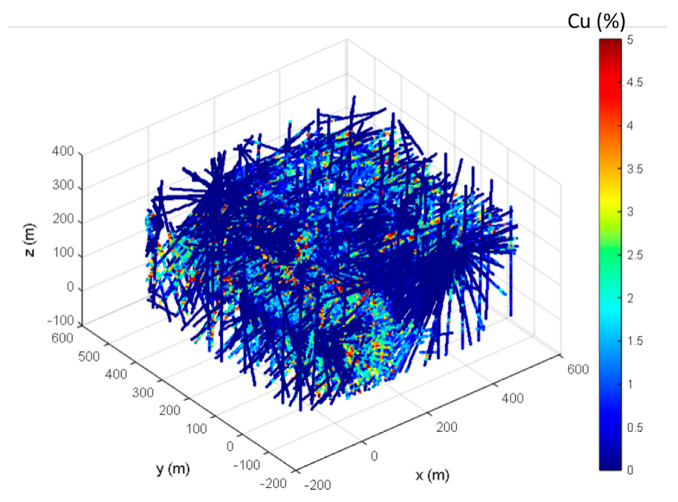
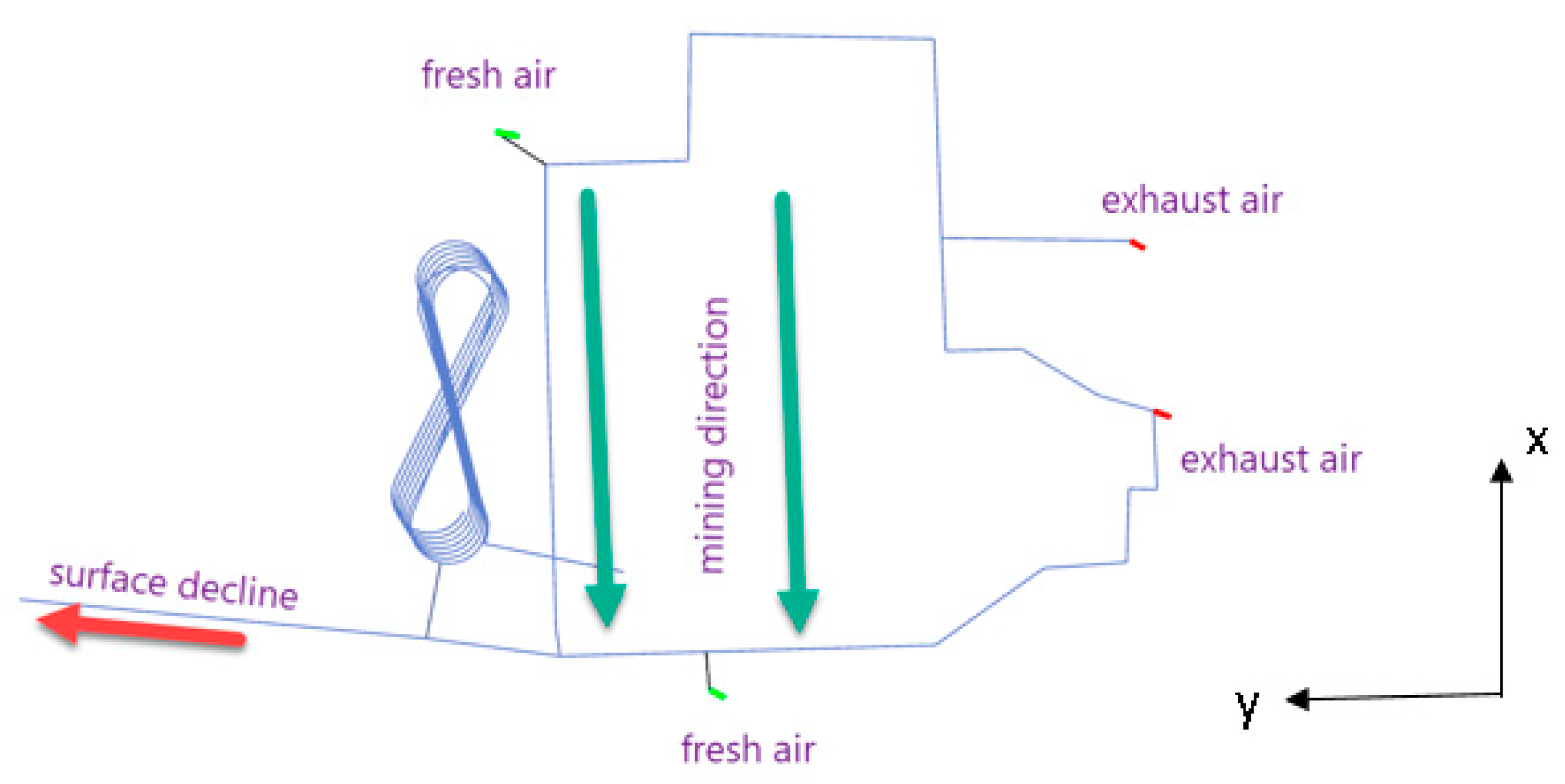
3. Case Study at an Operating Copper Mine

The case study presented herein shows first an analysis of the simulations produced by the high-order sequential simulation (HOSIM) method described in Section 2.2.1 and a comparison to sequential Gaussian simulations (SGS) of a copper deposit related to an operating underground copper mine. These simulations obtained through the HOSIM method are used as an input to the proposed extended integrated stochastic optimization of the underground mine design and production schedule with stockpiling, the extraction sequence, and the forecasts presented. A comparison between these outputs to the ones obtained with the same optimization framework and technical parameters, but with simulations generated with the SGS method, is subsequently shown.

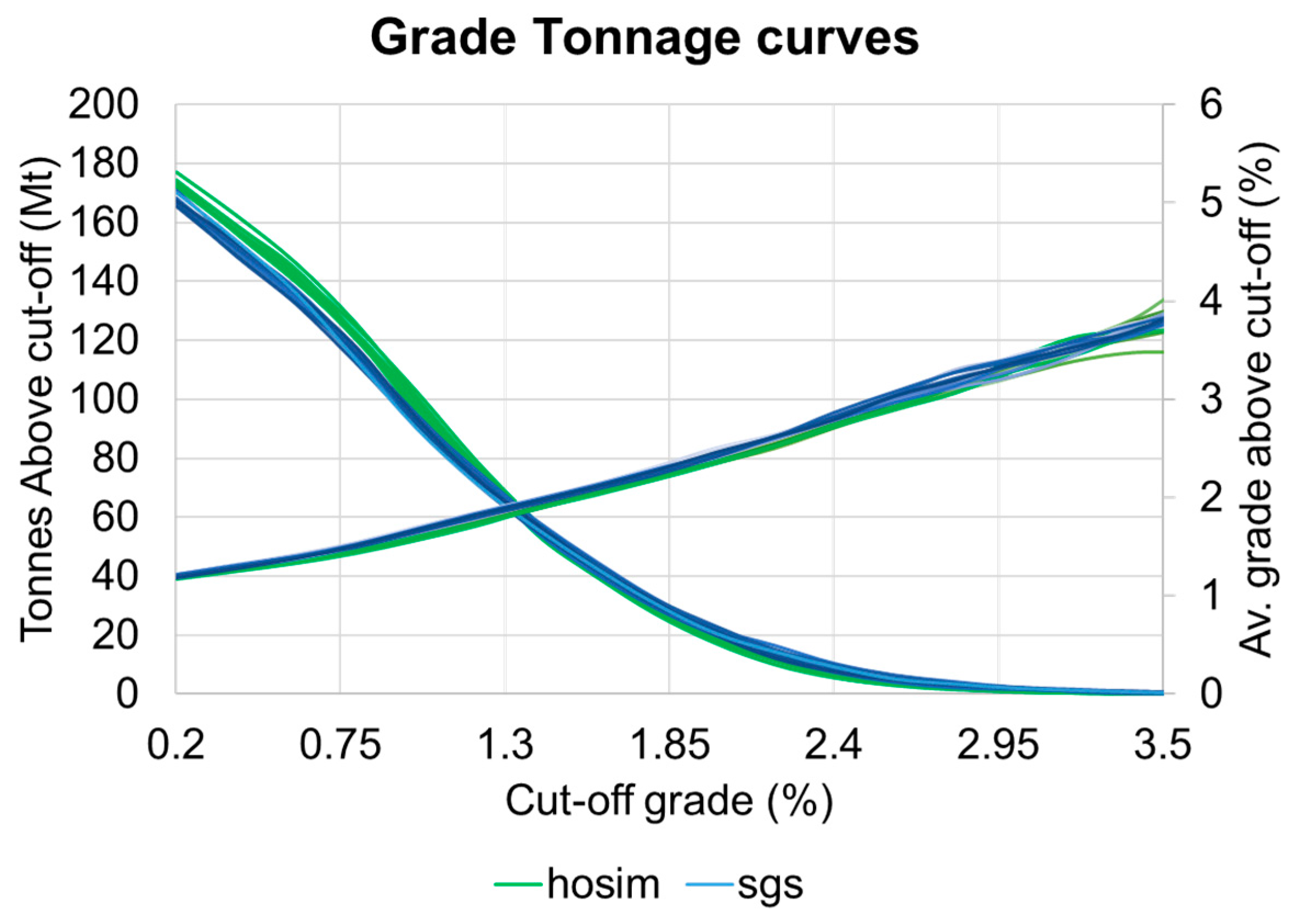
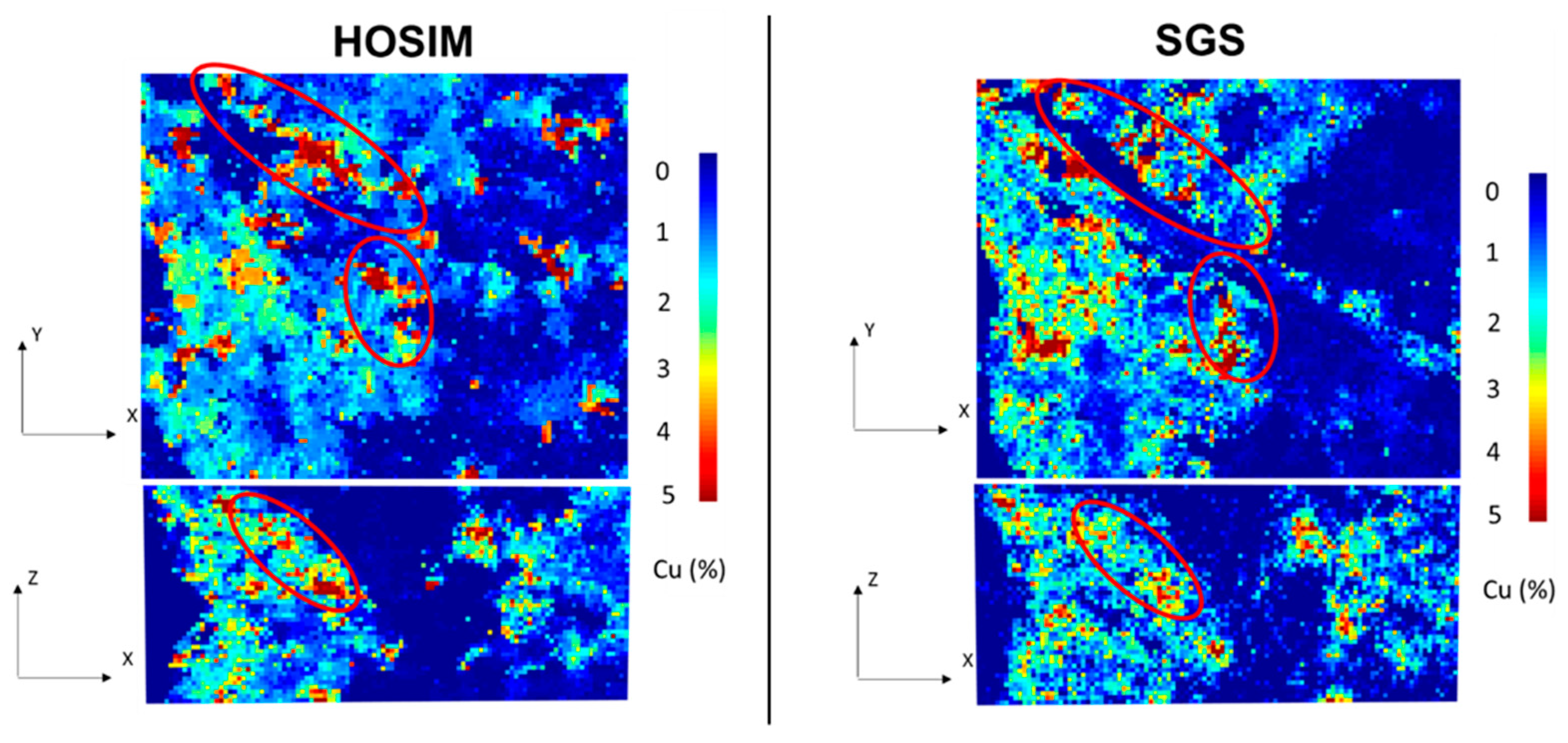
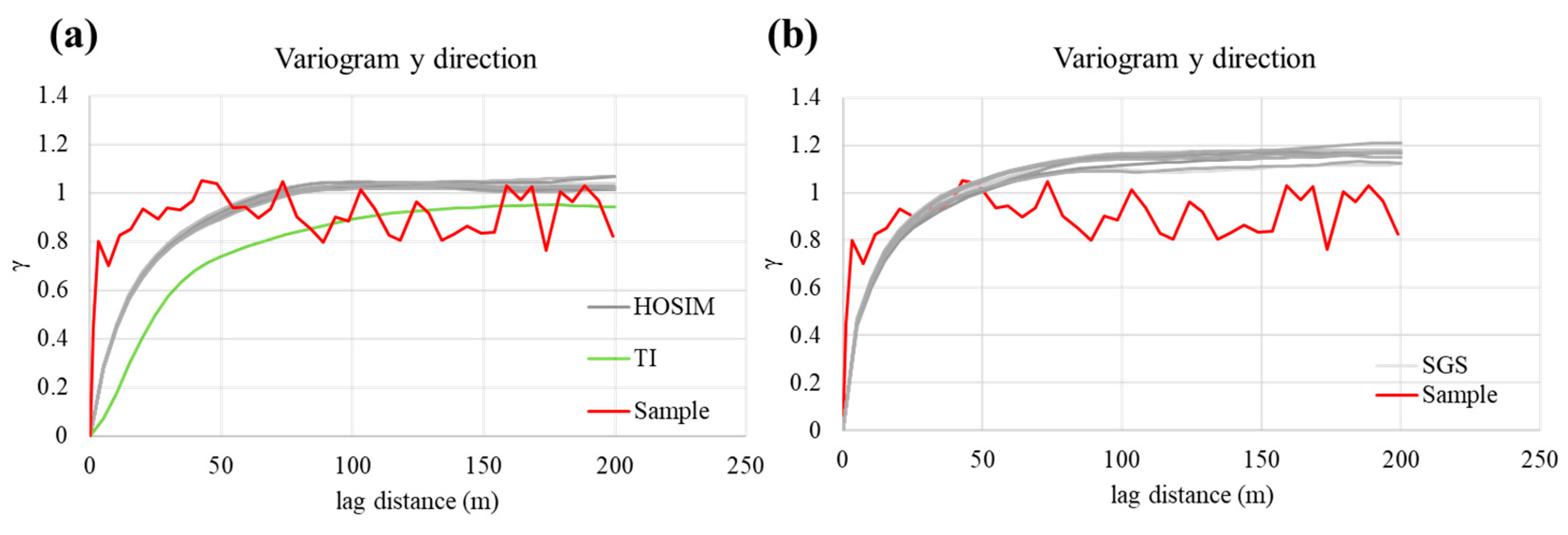
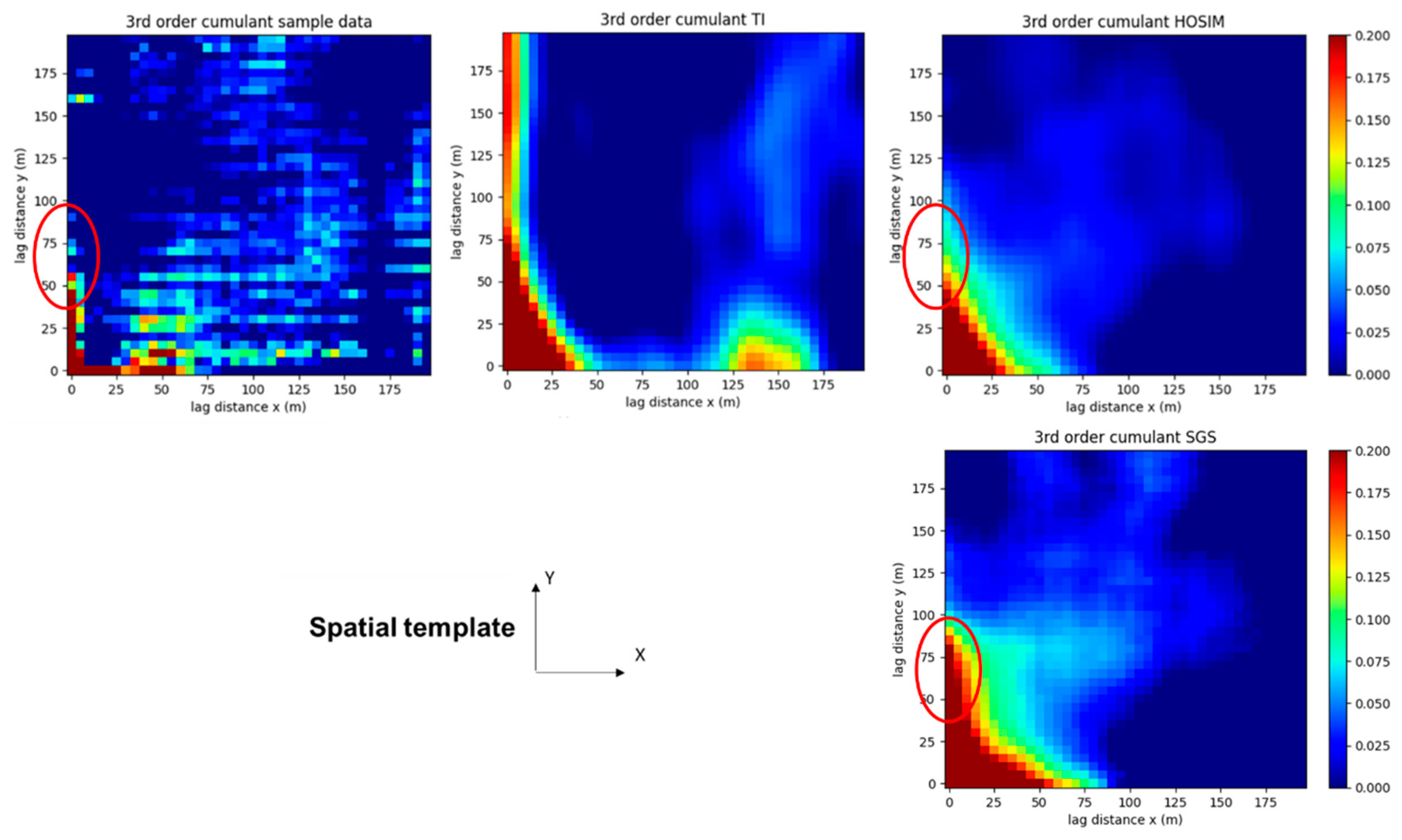
3.1. High-Order Sequential Simulations of the Mineral Deposit, Results and Comparisons to Sequential Gaussian Simulations

The realizations of the copper deposit using the high-order sequential simulation (HOSIM) method are conducted in a grid size of 5 m × 5 m × 5 m with 466,560 nodes. In order to generate the simulations, 1510 exploration drill holes with 5 m composites are spatially distributed as fans, with centers at approximately every 30 m, which are used as the sample data, as shown in Figure 3. In addition, a training image (TI) generated from densely sampled blast hole data was used. A set of 20 high-order sequential simulations is generated in point support and then goes through the previously described preprocessing steps to generate the inputs to the proposed optimization method. From this set, 10 simulations are used directly as an input to the optimization and the remaining 10 simulations are further used for the risk analysis of the related forecasts. The number of simulations follows previous studies that show that 10–12 simulations are sufficient to produce stable results for mine planning optimization [37,67,72].

Ten simulations of the copper deposit, using the same exploration data, are generated based on the sequential Gaussian simulation (SGS) method, to be used as a means of comparison to the ones obtained using HOSIM. Figure 4 shows the grade-tonnage curves for the two sequential simulation frameworks being compared, considering the minimum stope dimensions (i.e., 15 m × 30 m × 40 m). The blue and green curves in the graph overlap each other for some of the simulated scenarios indicating that, for both methods, the grade and tonnage proportions are similar. Thus, the simulation method does not directly impact the metal quantities. Figure 5 shows cross-sections of simulations using high-order and Gaussian sequential simulations. A visual inspection indicates that both realizations reproduce the spatial distribution of copper grades of the exploration data. However, the realization generated with the SGS shows a more dispersed behavior, representing the effect of maximum entropy when the data is transformed into Gaussian space. The highlighted high-grade areas show better connectivity for the realization generated with HOSIM, as expected.

The reproduction of spatial statistics of the simulations in terms of the exploration data is evaluated. Figure 6 shows the histograms of the sample data, TI, and high-order sequential simulation realizations. Similarly, Figure 7, Figure 8, Figure 9 and Figure 10 show the variograms in x and y directions, third- and fourth-order cumulant maps form the sample data, TI, and a realization produced by HOSIM and SGS methods. The areas with red circles highlight the main differences among the cumulant maps. It is seen that both methods can reasonably reproduce the histograms and variograms of the exploration data. For third- and fourth-order cumulants, however, the realization obtained with the HOSIM method shows a closer reproduction to the sample data, compared to what is shown for the realization obtained with the SGS method. In addition, although the described HOSIM method uses a TI to infer the conditional probability distribution function (cpdf), the simulated values reproduce the low and high-order statistics of the exploration (i.e., sample) data. In fact, the TI assumes an auxiliary part in the simulation procedure, while the initial sample data serves as conditioning data and is also used to calculate the cpdf.

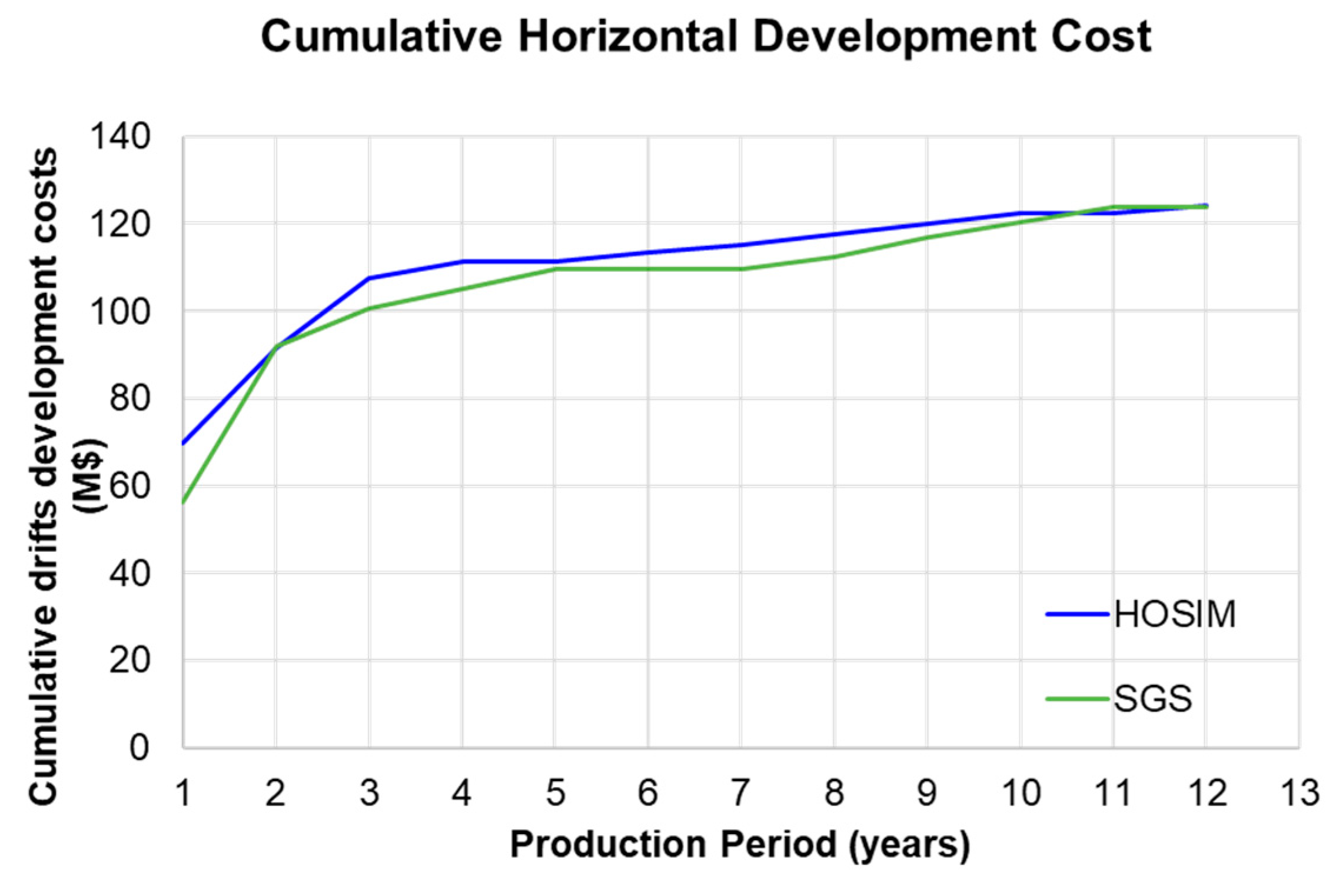
3.2. Integrated Stope Design and Scheduling Optimization and Forecasting

The application of the proposed integrated stochastic stope design and production scheduling with long-term stockpiling at a copper deposit is presented in this section. The comparison of the stope design, extraction sequence, and related forecasts using high-order and Gaussian sequential simulations presented in the previous section, are used as inputs to the optimization approach, the result of which is then analyzed.

The present case study is developed for an operating underground copper mine. Therefore, mine accesses (i.e., ramp and decline) and ventilation systems are given as inputs. Figure 11 shows the available infrastructure in the mine and the defined mining direction. In addition, geometrical parameters for the shapes of the stopes were provided by the mining company operating the mine. The maximum and minimum dimensions of the stopes are considered, given geotechnical and drilling equipment requirements, as shown in

Table 2. Stope geometrical parameters.

Parameter	Value/Description
Minimum dimensions	15 m × 30 m × 30 m
Maximum dimensions	30 m × 30 m × 150 m

. These possible configurations account for the position of the access point at each sublevel according to the available ramp design. Three option types are used as input, meaning that all stopes will have the possibility of being primary, secondary, or tertiary. In addition, the stopes are blasted and extracted bottom-up and are subsequently backfilled with cemented aggregate fill (CAF), which is not considered a limiting feature in mine production. Thus, a single mining cost is used for all stope types. A horizontal development capacity is considered in terms of the maximum length that can be developed. A single haulage system is available with its maximum capacity constraining the mining capacity, and a processor with a smaller capacity controls the copper concentrate product production. An annual stockpile capacity is considered in order to manage the grade blending, while uncertainty in terms of copper grades is taken into consideration. Thus, penalty costs for deviations from the minimum and maximum grades for this element’s requirements are applied and are discounted throughout the years to manage the geologic risk [70].

Table 3. Technical and economic parameters are used as input in the optimization.

Parameter	Value
Cu price	8500 $/t
Economic discount rate	10%
Geologic discount rate	10%
Processing recovery Cu	94%
Mining cost	50 $/t
Processing cost	13.5 $/t
Haulage cost	5 $/t×m
Rehandling cost	0.5 $/t
Drifts development cost	12,000 $/m
Density	3.2 t/m3
Haulage capacity	3 Mt/year
Processing capacity	2.5 Mt/year
Stockpiling capacity	400 kt/year
Drift development capacity	5000 m/year
Minimum copper mill head grade	1.8%
Penalty cost for deviations below minimum Cu mill head grade	100 $/unit

displays the technical and economic parameters used in the optimization of the copper mine. The proposed SIP model is programmed in the C++ language and solved using the CPLEX v.12.8.0 software’s solver engine [73].

Figure 12 displays the extraction sequence and the optimum stope types when the simulations generated with the HOSIM method are used. An operational extraction sequence that follows the mining direction and the bottom-up extraction approach, while respecting the adjacencies given by the optimized stope types is produced. The output results obtained with the high-order sequential simulations are compared to those obtained when the simulations generated using the SGS method are the inputs. Similar to Figure 12, Figure 13 displays the extraction sequence and the optimum stope types when the simulations generated with the SGS method are used. It is observed that, although for both cases the same parameters are considered, the extraction sequence displayed in Figure 12 and Figure 13 are different, and relevant differences can be noticed on the final stope layout. Once the simulated grades are averaged into possible stope volumes, the more connected the high grades are, the higher the stope grades will be. When the simulations generated by the HOSIM method are used as inputs, areas further to the access point can be mined, once the profit generated from the metal content of this stope prevails over the cumulative horizontal development costs. On the other hand, when sequential Gaussian simulations are used, it is observed that the stopes closer to the access points are preferred once they incur lower development costs, as highlighted with the red circles Additionally, when the realizations generated by HOSIM are used, smaller stope sizes are chosen, allowing more selectivity in terms of high-grade stopes and less dilution.

Figure 14 shows the risk profiles considering the decisions optimized using the different inputs with 10 additional high-order sequential simulations. The results are presented in terms of P10, P50, and P90, representing the 10th, 50th, and 90th percentiles of the related performance indicators, respectively. Figure 14a shows that the produced copper content is 4% higher when the realization generated with the HOSIM method is the related input. This can be explained by the maximum entropy that the Gaussian-based approaches generate with respect to the high grades. Thus, after the optimization process, it is observed that the high-grade areas are a better target when a better representation of extreme grade continuity is given as input. The copper production impacts directly on the NPV, which is 6% higher for the HOSIM case compared to the SGS case, as shown in Figure 14b. Although the mined tonnage is similar for both cases (Figure 14c), the cumulative stockpiled tonnage is approximately 5% higher for the SGS case (Figure 14e), which means that the use of the stockpile is necessary to achieve the grade blending requirements, incurring higher rehandling costs. Figure 14d shows that grade blending requirements are overall achieved for both cases, with probable deviations from the lower bound for the SGS case. As previously inferred from the extraction sequences (Figure 12 and Figure 13), in the SGS case, the areas closer to the access points are privileged. In the graph displayed in Figure 15, the horizontal development costs for the SGS case are, in fact, lower for early periods. However, the total horizontal development cost is similar for both cases. Considering the ability of the optimization process to decide whether to stockpile mined material or not and when over the life of this mine, the analysis demonstrates that, in both scenarios, it is profitable to direct material to stockpiles, given the associated rehandling costs. This strategic choice results in an optimal NPV and minimum deviations from the required lower bound of copper grade. Figure 16 shows the number of active stockpiles and tonnage left at the stockpiles for each period and for each case, assuming that multiple stockpiles can be used to assist in the selection of the stockpiled material to be processed. The maximum yearly stockpiling capacity of 400,000 tons is respected and a maximum of three active stockpiles are needed for both cases. This finding underscores the significant role of stockpiling decisions in long-term mine planning, as they can conform to operational considerations and requirements.

4. Conclusions

The paper proposes an extension of previous work on the integrated stochastic optimization of stope design and mine production scheduling, through a two-stage stochastic integer programming (SIP) linear formulation that accounts for long-term stockpiling decisions for the sublevel open stoping (SLOS) mining method. The operational aspects and impacts on the mine production scheduling with this additional component are evaluated. The objective function of the proposed SIP aims to maximize the net present value (NPV) of the project while managing the geological uncertainty, by minimizing deviations from production targets, subjected to operational constraints are presented. Additionally, the effects of using the high-order sequential simulation (HOSIM) method to generate the realizations of a copper deposit to be used as inputs for the proposed stochastic optimization formulation are also presented. This simulation method infers high-order spatial statistics from available data, enabling the reproduction of complex geological patterns of natural phenomena. The optimized stope design and production schedule along with the related forecasts are compared against a case where the conventional sequential Gaussian simulations are the main inputs for the optimization formulation. It is observed that these simulation methods can be fairly compared against each other once they produce similar grade-tonnage proportions and reproduce related statistics, that is, histograms and variograms of the available sample data. It is seen, however, that, due to the maximum entropy property of the Gaussian-based methods, the extremely high grades are more spatially dispersed, showing a misrepresentation of the spatial connectivity of the high grades. It is also verified that the realizations obtained with the HOSIM method reproduce the sample data high-order spatial statistics despite the utilization of a training image (TI).

The application of the proposed method shows that long-term stockpiles can be operationally implemented. Under the assumption of having multiple active stockpiles, to facilitate operational mining aspects, it is seen that a maximum of three active stockpiles are needed and the stockpile tonnage after each production year does not reach the maximum capacity of 400,000 tones in both the HOSIM and SGS input cases. In addition, it is observed that the optimization process takes advantage of the more connected high-grade representations of the copper deposit to generate the stope designs production schedules. Notable differences are observed on the final stope boundaries and extraction sequences comparing the two cases. The HOSIM case tends to target the high-grade continuity areas to produce a 6% higher NPV, while the SGS case initially mines areas that incur a smaller horizontal development cost. This outcome is observed once the simulated values are averaged into large stope volumes; thereafter, the realizations with better connected high grades generate higher-grade possible stopes. As a result, the higher the stope grade, the lower the impact of the horizontal development cost on its profit. The HOSIM case produces a 4% higher copper content at the end of 12 years of production, which directly impacts on the cumulative cash flow. In addition, the HOSIM case is able to produce ore material that follows the grade-blending requirement of the mill by sending 5% less material to the stockpile.

A case study that accounts for high-order sequential simulations of multiple elements is a topic for future research, once secondary and deleterious elements also play an important role in decision-making for mine planning activities. In addition, the simultaneous optimization of a mining complex that assumes the existence of multiple mines, stockpiles, and processing streams is an extension for future work. Also, this simultaneous optimization approach should generalize to different types of underground mining methods, while further facilitating the interaction between underground and open-pit mining operations. Furthermore, as more components are included in the mathematical programming formulation, the development of alternative solvers, rather than the ones commercially available, is proposed for future contribution. The proposed method addresses long-term underground stope design, mine planning, and production scheduling. However, it is recognized that intricate operational considerations, such as the scheduling of individual activities, prediction of technical parameters, and updates on geotechnical parameters, are important for short-term planning. Future developments related to short-term planning could consider integrating these aspects as well as enabling the interaction between short and long-term planning.

References

1. Hamrin, H. Underground mining methods and applications. In Underground Mining Methods: Engineering Fundamentals and International Case Studies; Hamrin, H., Hustrulid, W., Bullock, R., Eds.; Society for Mining, Metallurgy and Exploration (SME): Littleton, CO, USA, 2001; pp. 3–14. [Google Scholar]
2. Hartman, H.L.; Mutmansky, J.M. Introductory Mining Engineering, 2nd ed.; John Wiley & Sons, Inc.: Hoboken, NJ, USA, 2002. [Google Scholar]
3. Pakalnis, R.; Hughes, P.B. Sublevel stoping. In SME Mining Engineering Handbook; Darling, P., Ed.; Society for Mining, Metallurgy, and Exploration, Inc.: Englewood, CO, USA, 2011; pp. 1355–1363. [Google Scholar]
4. Alford, C. Optimisation in underground mine design. In Proceedings of APCOM XXV: Application of Computers and Operations Research in the Minerals Industries; AusIMM: Melbourne, Australia, 1995; pp. 213–218. [Google Scholar]
5. Alford, C.; Hall, B. Stope optimisation tools for selection of optimum cut-off grade in underground mine design. In Project Evaluation Conference; AusIMM: Melbourne, Australia, 2009; pp. 137–144. [Google Scholar]
6. Alford Mining Systems. AMS—Stope Shape Optimizer; Carlton: Victoria, Australia, 2022. [Google Scholar]
7. Cawrse, I. Multiple pass floating stope process. In Strategic Mine Planning Conference; AusIMM Publication Series: Perth, Australia, 2001; pp. 87–94. [Google Scholar]
8. Erdogan, G.; Cigla, M.; Topal, E.; Yavuz, M. Implementation and comparison of four stope boundary optimization algorithms in an existing underground mine. Int. J. Min. Reclam. Environ. 2017, 31, 389–403. [Google Scholar] [CrossRef]
9. Nikbin, V.; Mardaneh, E.; Asad, M.W.A.; Topal, E. Pattern search method for accelerating Stope boundary optimization problem in underground mining operations. Eng. Optim. 2021, 54, 881–893. [Google Scholar] [CrossRef]
10. Brazil, M.; Grossman, P.A.; Lee, D.H.; Rubinstein, J.H.; Thomas, D.A.; Wormald, N.C. Decline design in underground mines using constrained path optimisation. Min. Technol. 2008, 117, 93–99. [Google Scholar] [CrossRef]
11. Brazil, M.; Lee, D.H.; Van Leuven, M.; Rubinstein, J.H.; Thomas, D.A.; Wormald, N.C. Optimising declines in underground mines. Min. Technol. 2003, 112, 164–170. [Google Scholar] [CrossRef]
12. Brazil, M.; Thomas, D.A. Network optimization for the design of underground mines. Networks 2007, 49, 40–50. [Google Scholar] [CrossRef]
13. Brickey, A.J. Undergrounf Production Scheduling Optimization with Ventilation Constraints; Colorado School of Mines: Golden, CO, USA, 2015; pp. 1–93. [Google Scholar]
14. Fava, L.; Millar, D.; Maybee, B. Scenario evaluation through mine schedule optimisation. In Proceedings of the 2nd International Seminar on Mine Planning, Antofagasta, Chile, 8–10 June 2011; pp. 1–10. [Google Scholar]
15. Fava, L.; Saavedra-Rosas, J.; Tough, V.; Haarala, P. A heuristic optimization process for achieving strategic mine planning targets. In Proceedings of the 23rd World Mining Congress, Montreal, QC, Canada, 11–15 August 2013. [Google Scholar]
16. Hauta, R.; Whittier, M.; Fava, L. Application of the geosequencing module to ensure optimised underground mine schedules with reduced geotechnical risk. In Underground Mining Technology 2017; Hudyma, M., Potivin, Y., Eds.; Australian Centre for Geomechanics (ACG): Sudbury, ON, Canada, 2017; pp. 547–555. [Google Scholar]
17. Little, J.; Topal, E.; Knights, P. Simultaneous optimisation of stope layouts and long term production schedules. Min. Technol. 2011, 120, 129–136. [Google Scholar] [CrossRef]
18. Newman, A.M.; Rubio, E.; Caro, R.; Weintraub, A.; Eurek, K. A review of operations research in mine planning. Inf. J. Appl. Anal. 2010, 40, 222–245. [Google Scholar] [CrossRef]
19. Topal, E. Advanced Underground Mine Scheduling Using Mixed Integer Programming; Colorado School of Mines: Golden, Colorado, USA, 2003. [Google Scholar]
20. Trout, L. Underground mine production scheduling using mixed integer programming. In Application of Computers and Operations Research in the Mineral Industry (APCOM); Australasian Institute of Mining and Metallurgy: Brisbane, Australia, 1995; pp. 395–400. [Google Scholar]
21. Chimunhu, P.; Topal, E.; Ajak, A.D.; Asad, W. A review of machine learning applications for underground mine planning and scheduling. Resour. Policy 2022, 77, 102693. [Google Scholar] [CrossRef]
22. Campeau, L.-P.; Gamache, M.; Martinelli, R. Integrated optimisation of short- and medium-term planning in underground mines. Int. J. Min. Reclam. Environ. 2022, 36, 235–253. [Google Scholar] [CrossRef]
23. Martinelli, R.; Collard, J.; Gamache, M. Strategic planning of an underground mine with variable cut-off grades. Optim. Eng. 2020, 21, 803–849. [Google Scholar] [CrossRef]
24. Ravenscroft, P.J. Risk analysis for mine scheduling by conditional simulation. Trans. Inst. Min. Metall. 1992, 101, A104–A108. [Google Scholar]
25. Dowd, P. Risk assessment in reserve estimation and open-pit planning. Trans. Inst. Min. Metall. Sect. A Min. Technol. 1994, 103, 148–154. [Google Scholar]
26. Grieco, N.; Dimitrakopoulos, R. Managing grade risk in stope design optimisation: Probabilistic mathematical programming model and application in sublevel stoping. Min. Technol. 2007, 116, 49–57. [Google Scholar] [CrossRef]
27. Little, J.; Knights, P.; Topal, E. Integrated optimization of underground mine design and scheduling. J. South. Afr. Inst. Min. Metall. 2013, 113, 775–785. [Google Scholar]
28. Copland, T.; Nehring, M. Integrated optimization of stope boundary selection and scheduling for sublevel stoping operations. J. S. Afr. Inst. Min. Metall. 2016, 116, 1135–1142. [Google Scholar] [CrossRef]
29. Foroughi, S.; Hamidi, J.K.; Monjezi, M.; Nehring, M. The integrated optimization of underground stope layout designing and production scheduling incorporating a non-dominated sorting genetic algorithm (NSGA-II). Resour. Policy 2019, 63, 101408. [Google Scholar] [CrossRef]
30. Hou, J.; Li, G.; Hu, N.; Wang, H. Simultaneous integrated optimization for underground mine planning: Application and risk analysis of geological uncertainty in a gold deposit. Gospod. Surowcami Miner.-Miner. Resour. Manag. 2019, 35, 153–174. [Google Scholar] [CrossRef]
31. Furtado e Faria, M.; Dimitrakopoulos, R.; Lopes Pinto, C.L. Integrated stochastic optimization of stope design and long-term underground mine production scheduling. Resour. Policy 2022, 78, 102918. [Google Scholar] [CrossRef]
32. Birge, J.R.; Louveaux, F. Introduction to Stochastic Programming; Springer: New York, NY, USA, 2011. [Google Scholar]
33. Carelos Andrade, L.; Dimitrakopoulos, R.; Cownway, P. Integrated stochastic optimization of stope design and long-term production scheduling at an operating underground copper mine. Int. J. Min. Reclam. Environ. 2023, 78, 102918. [Google Scholar]
34. Villaescusa, E. Geotechnical Design for Sublevel Open Stoping; CRC Press, Taylor & Francis Group: New York, NY, USA, 2014. [Google Scholar]
35. Skipochka, S.I.; Palamarchuk, T.A.; Sergienko, V.N. Geomechanical monitoring for underground mining mineral deposits. In Innovative Development of Resource-Saving Technologies for Mining; Multi-authores monograph; Kalinichenko, V.A., Ed.; Publishing House “St.Ivan Rilski”: Sofia, Ukraine, 2018; pp. 147–167. [Google Scholar]
36. Dimitrakopoulos, R. (Ed.) Advances in Applied Strategic Mine Planning, 1st ed.; Springer Nature: Cham, Switzerland, 2018; pp. 1–802. [Google Scholar]
37. Dimitrakopoulos, R.; Lamghari, A. Simultaneous stochastic optimization of mining complexes—Mineral value chains: An overview of concepts, examples and comparisons. Int. J. Min. Reclam. Environ. 2022, 36, 443–460. [Google Scholar] [CrossRef]
38. Goodfellow, R.; Dimitrakopoulos, R. Global optimization of open pit mining complexes with uncertainty. Appl. Soft Comput. 2016, 40, 292–304. [Google Scholar] [CrossRef]
39. Dimitrakopoulos, R.; Grieco, N. Stope design and geological uncertainty: Quantification of risk in conventional designs and a probabilistic alternative. J. Min. Sci. 2009, 45, 152–163. [Google Scholar] [CrossRef]
40. Villalba Matamoros, M.E.; Kumral, M. Underground mine planning: Stope layout optimisation under grade uncertainty using genetic algorithms. Int. J. Min. Reclam. Environ. 2018, 33, 353–370. [Google Scholar] [CrossRef]
41. Furtado e Faria, M.; Dimitrakopoulos, R.; Lopes Pinto, C.L. Stochastic stope design optimisation under grade uncertainty and dynamic development costs. Int. J. Min. Reclam. Environ. 2022, 36, 81–103. [Google Scholar] [CrossRef]
42. Carpentier, S.; Gamache, M.; Dimitrakopoulos, R. Underground long-term mine production scheduling with integrated geological risk management. Min. Technol. 2016, 125, 93–102. [Google Scholar] [CrossRef]
43. Dirkx, R.; Kazakidis, V.; Dimitrakopoulos, R. Stochastic optimisation of long-term block cave scheduling with hang-up and grade uncertainty. Int. J. Min. Reclam. Environ. 2018, 33, 371–388. [Google Scholar] [CrossRef]
44. Goovaerts, P. Geostatistics for Natural Resources Evaluation; Oxford University Press: New York, NY, USA, 1997. [Google Scholar]
45. Chilès, J.-P.; Delfiner, P. Geostatistics; Wiley Series in Probability and Statistics: Hoboken, NJ, USA, 1999. [Google Scholar]
46. Rossi, M.E.; Deutsch, V. Mineral Rosource Estimation, 1st ed.; Springer: Dordrecht, The Netherlands, 2014. [Google Scholar]
47. David, M. Hadbook of Applied Advanced Geostatistical Ore Reserve Estimation; Elsevier: Amsterdam, The Netherlands, 1988. [Google Scholar]
48. Journel, A.G.; Huijbregts, C.J. Mining Geostatistics; Academic Press: London, UK, 1978. [Google Scholar]
49. Mariethoz, G.; Caers, J. Multiple-Point Geostatistics: Stochastic Modeling with Training Images; Wiley-Blackwell: New York, NY, USA, 2015; p. 384. [Google Scholar]
50. Journel, A.G. Modeling uncertainty: Some conceptual thoughts. In Geostatistics for the Next Century; Dimitrakopoulos, R., Ed.; Springer: Dordrecht, The Netherlands; Montreal, QC, Canada, 1994; pp. 30–43. [Google Scholar]
51. Journel, A.G.; Deutsch, C.V. Entropy and spatial disorder. Math. Geol. 1993, 25, 329–355. [Google Scholar] [CrossRef]
52. Dimitrakopoulos, R.; Mustapha, H.; Gloaguen, E. High-order statistics of spatial random fields: Exploring spatial cumulants for modeling complex non-Gaussian and non-linear phenomena. Math. Geosci. 2010, 42, 65–99. [Google Scholar] [CrossRef]
53. Journel, A.G. Beyond covariance: The advent of multiple-point geostatistics. In Geostatistics Banff 2004; Leuangthong, O., Deutsch, C.V., Eds.; Springer: Dordrecht, The Netherlands; Banff, AB, Canada, 2005; pp. 225–233. [Google Scholar]
54. Remy, N.; Alexandre, B.; Wu, J. Applied Geostatistics with SGems: A User’s Guide; Cambridge University Press: Cambrigde, UK, 2009. [Google Scholar]
55. Guardiano, F.; Srivasta, R. Multivariate geostatistics: Beyond bivariate moments. In Geostatistics Troia ‘92; Soares, A., Ed.; Springer: Dordrecht, The Netherlands, 1993; pp. 133–144. [Google Scholar]
56. Strebelle, S. Conditional simulation of complex geological structures using multiple-point statistics. Math. Geol. 2002, 34, 1–21. [Google Scholar] [CrossRef]
57. Arpat, G.B.; Caers, J. Conditional simulation with patterns. Math. Geol. 2007, 39, 177–203. [Google Scholar] [CrossRef]
58. Zhang, T.; Switzer, P.; Journel, A. Filter-based classification of training image patterns for spatial simulation. Math. Geol. 2006, 38, 63–80. [Google Scholar] [CrossRef]
59. Mariethoz, G.; Renard, P.; Straubhaar, J. The direct sampling method to perform multiple-point geostatistical simulations. Water Resour. Res. 2010, 46, W11536. [Google Scholar] [CrossRef]
60. Osterholt, V.; Dimitrakopoulos, R. Simulation of orebody geology with multiple-point geostatistics—Application at Yandi Channel iron ore deposit, WA, and implications for resource uncertainty. In Advances in Applied Strategic Mine Planning; Dimitrakopoulos, R., Ed.; Springer Nature: Cham, Switzerland, 2018; pp. 335–352. [Google Scholar]
61. Minniakhmetov, I.; Dimitrakopoulos, R.; Godoy, M. High-order spatial simulation using legendre-like orthogonal splines. Math. Geosci. 2018, 50, 753–780. [Google Scholar] [CrossRef] [PubMed]
62. Mustapha, H.; Dimitrakopoulos, R. HOSIM: A high-order stochastic simulation algorithm for generating three-dimensional complex geological patterns. Comput. Geosci. 2011, 37, 1242–1253. [Google Scholar] [CrossRef]
63. de Carvalho, J.P.; Dimitrakopoulos, R.; Minniakhmetov, I. High-order block support spatial simulation method and its application at a gold deposit. Math. Geosci. 2019, 51, 793–810. [Google Scholar] [CrossRef]
64. Dimitrakopoulos, R.; Yao, L. High-order spatial stochastic models. In Encyclopedia of Mathematical Geosciences; Daya Sagar, B.S., Cheng, Q., McKinley, J., Agterberg, F., Eds.; Springer: Cham, Switzerland, 2020; pp. 1–10. [Google Scholar]
65. de Carvalho, J.P.; Dimitrakopoulos, R. Effects of high-order simulations on the simultaneous stochastic optimization of mining complexes. Minerals 2019, 9, 210. [Google Scholar] [CrossRef]
66. Goodfellow, R.; Dimitrakopoulos, R. Simultaneous stochastic optimization of mining complexes and mineral value chains. Math. Geosci. 2017, 49, 341–360. [Google Scholar] [CrossRef]
67. Montiel, L.; Dimitrakopoulos, R. A heuristic approach for the stochastic optimization of mine production schedules. J. Heuristics 2017, 23, 397–415. [Google Scholar] [CrossRef]
68. Montiel, L.; Dimitrakopoulos, R. Optimizing mining complexes with multiple processing and transportation alternatives: An uncertainty-based approach. Eur. J. Oper. Res. 2015, 247, 166–178. [Google Scholar] [CrossRef]
69. Brika, Z. Optimisation de la Planification Stratégique d’une Mine à ciel Ouvert en Tenant Compte de L’incertitude Géologique; Department of Mathematics and Industrial Engineering, Polytechnique Montréal: Montreal, QC, Canada, 2019. [Google Scholar]
70. Ramazan, S.; Dimitrakopoulos, R. Production scheduling with uncertain supply: A new solution to the open pit mining problem. Optim. Eng. 2013, 14, 361–380. [Google Scholar] [CrossRef]
71. Isaaks, E. The Application of Monte Carlo Methods to the Analysis of Spatially Correlated Data; Stanford University: Stanford, CA, USA, 1990. [Google Scholar]
72. Albor Consuegra, F.R.; Dimitrakopoulos, R. Stochastic mine design optimisation based on simulated annealing: Pit limits, production schedules, multiple orebody scenarios and sensitivity analysis. Min. Technol. 2009, 118, 79–90. [Google Scholar] [CrossRef]
73. IBM ILOG. CPLEX User’s Manual; IBM: Armonk, NY, USA, 2017; p. 596. [Google Scholar]
Disclaimer/Publisher’s Note: The statements, opinions, and data contained in all publications are solely those of the individual author(s) and contributor(s) and not of MDPI and/or the editor(s). MDPI and/or the editor(s) disclaim responsibility for any injury to people or property resulting from any ideas, methods, instructions, or products referred to in the content.
Figure 1. Steps of the stope design and scheduling optimization.
Minerals 14 00123 g001
Figure 2. Stope type option,  a a , and  a  for different mining zone configurations  b  and  b .
Minerals 14 00123 g002
Figure 3. Exploration data with underground drilling fans.
Minerals 14 00123 g003
Figure 4. Grade-tonnage curves for simulated copper deposit using SGS and HOSIM, for stopes 15 × 30 × 40 m3.
Minerals 14 00123 g004
Figure 5. Cross-sections of the simulations, where high-grade areas are highlighted in red.
Minerals 14 00123 g005
Figure 6. Histograms of samples (red), TI (green), (a) HOSIM realizations (grey), and (b) SGS realizations (blue).
Minerals 14 00123 g006
Figure 7. Variograms in x direction of samples (red), TI (green), (a) HOSIM realizations (grey), and (b) SGS realizations (grey).
Minerals 14 00123 g007
Figure 8. Variograms in y direction of samples (red), TI (green), (a) HOSIM realizations (grey), and (b) SGS realizations (grey).
Minerals 14 00123 g008
Figure 9. Third-order cumulant maps of sample data, the used TI, HOSIM simulated realization, and SGS simulated realization, where areas highlighted in red show differences in cumulative maps.
Minerals 14 00123 g009
Figure 10. Fourth-order cumulant maps of sample data, the used TI, HOSIM simulated realization, and SGS simulated realization, where areas highlighted in red show differences in cumulative maps.
Minerals 14 00123 g010
Figure 11. Plan view of the developed infrastructure, where the green arrow indicates the mining direction and the red arrow indicates the direction to the surface decline.
Minerals 14 00123 g011
Figure 12. (a) Extraction sequence and (b) final stope types using input realization from HOSIM, red circles highlight the correspondent high-grade areas.
Minerals 14 00123 g012
Figure 13. (a) Extraction sequence and (b) final stope types using input realization from SGS, red circles highlight the correspondent high-grade areas.
Minerals 14 00123 g013
Figure 14. Risk profiles for (a) cumulative recovered copper, (b) NPV, (c) total tonnages mined, (d) mill copper head grade, and (e) cumulative stockpiled tonnage.
Minerals 14 00123 g014
Figure 15. Cumulative development costs for drifts and crosscuts.
Minerals 14 00123 g015
Figure 16. Number of active stockpiles (vertical columns) and tonnage left at the stockpiled for each period (dashed lines).
Minerals 14 00123 g016