
Prediction of Au-Polymetallic Deposits Based on Spatial Multi-Layer Information Fusion by Random Forest Model in the Central Kunlun Area of Xinjiang, China
 ,
,
Abstract
:1. Introduction
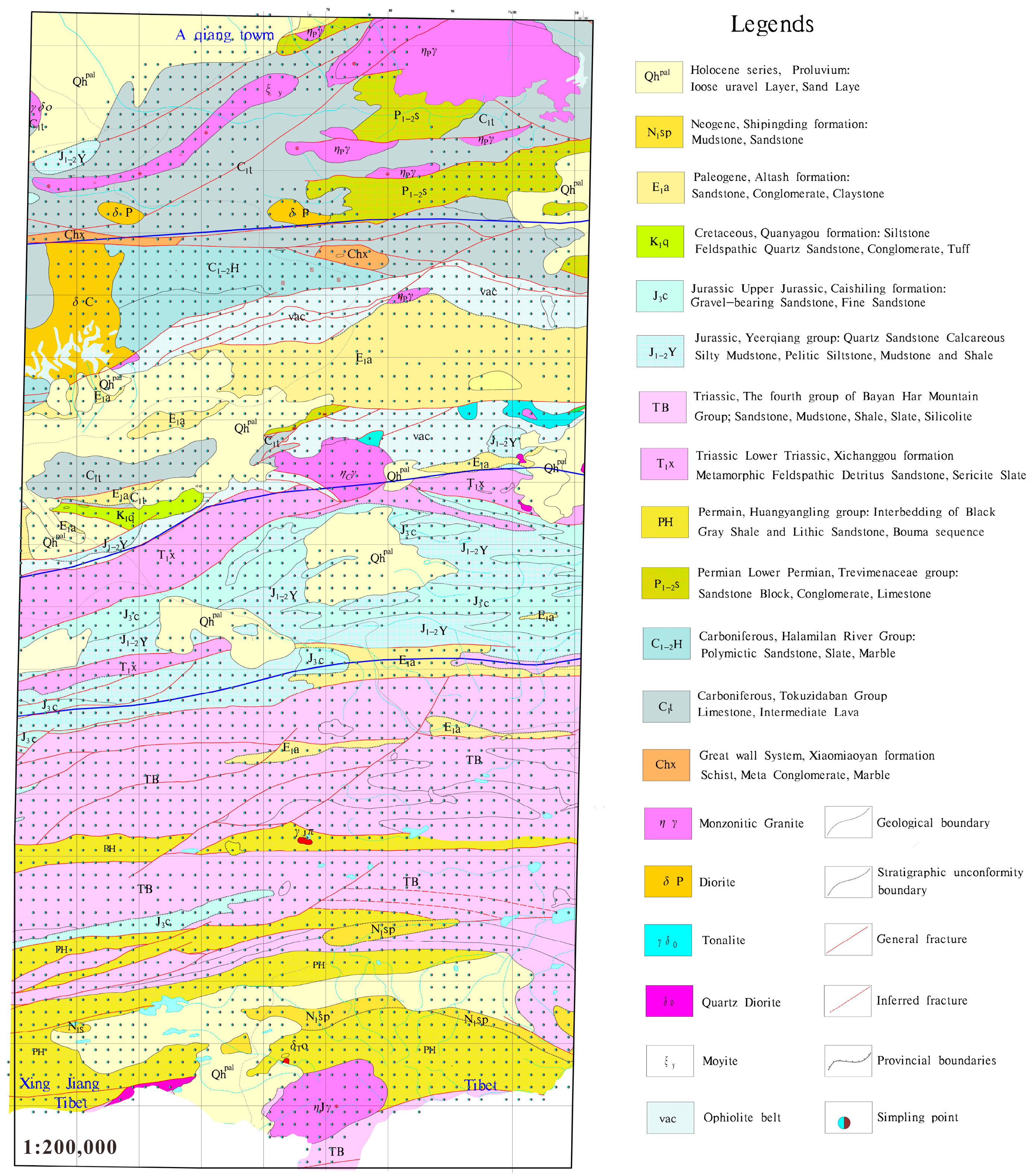
2. Regional Geology
2.1. Basic Geological Background
2.2. Metallogenic Belt
2.2.1. Karamiran (Compound Gully Arc Belt) Au–Cu–Ag Ore Belt
2.2.2. Huangyangling (Fold Belt) Sb–Hg–Au–Cu Ore Belt
2.2.3. Yunwuling (Fold Belt) Cu–Au Ore Belt
2.3. Characteristics of Mineral Resources
2.3.1. Sedimentary Type
2.3.2. Volcanic Type
2.3.3. Skarn Type
3. Data Sources and Main Research Methods
3.1. Data Sources and Introduction
3.2. Random Forest Algorithm (RF)
3.2.1. Undersampling Method
| Algorithm 1: Ensemble undersampling |
| Input: The training sample is the majority class sample, is the minority class sample; Base learner Training rounds T. Output: Integrated model N. Process: 1: for t = 1,2,…,T do 2: The subset is randomly selected from , and the size of the subset is consistent with 3: We use the base learner to train a single model on the dataset : 4: end for 5: Integration of results |
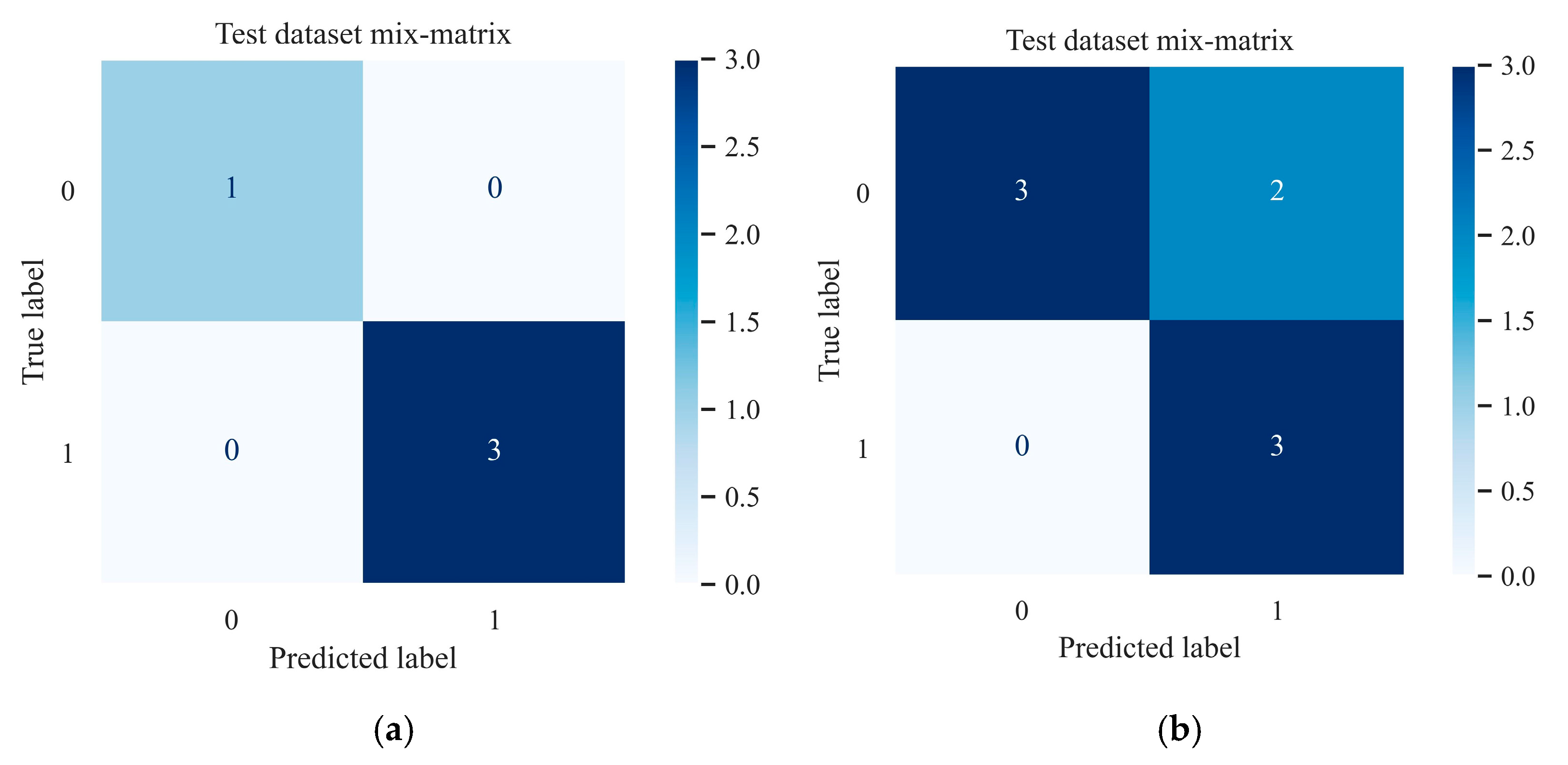
3.2.2. Performance Evaluation Parameters
3.2.3. Hold-Out Test
4. Metallogenic Prediction and Target Area Delineation of Au Polymetallic Deposits
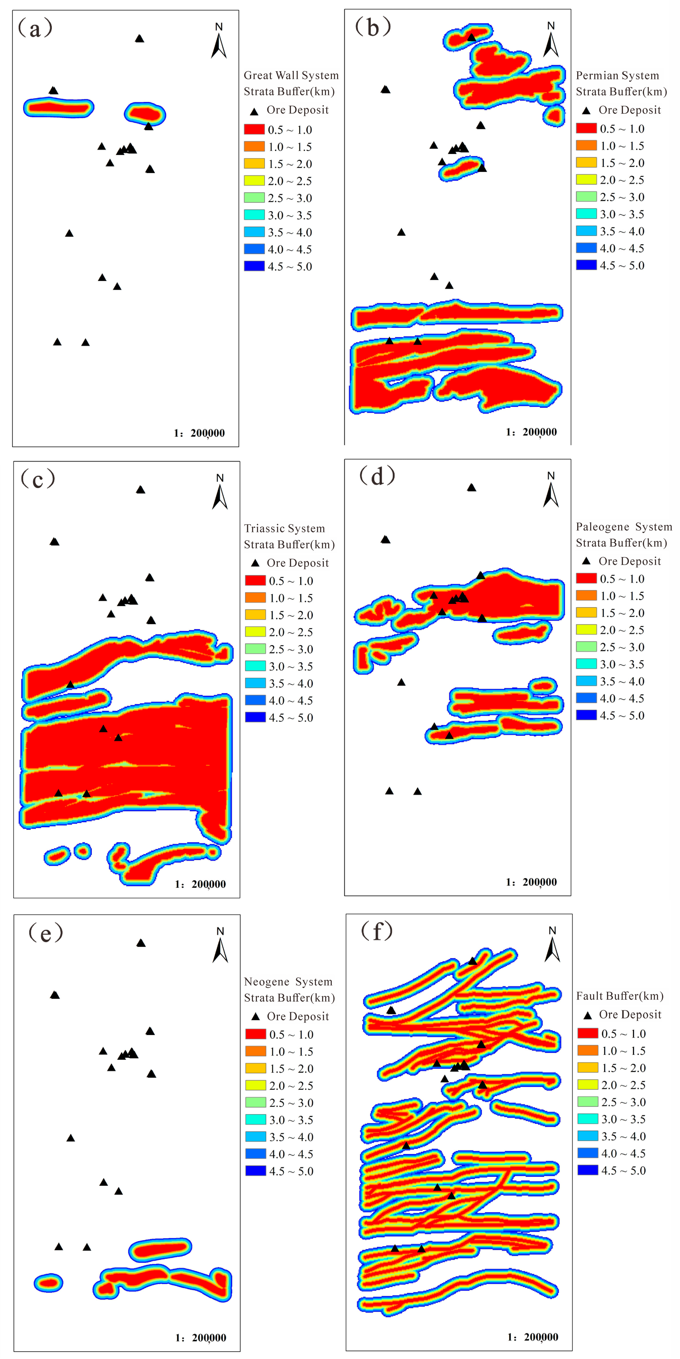
4.1. Geochemical Characteristics of Different Geological Units
4.1.1. Great Wall System (Ch)
4.1.2. Permian System (P)
4.1.3. Triassic System (T)
4.1.4. Paleogene System (E)
4.1.5. Neogene System (N)
4.2. Data Preprocessing and Dataset Establishment
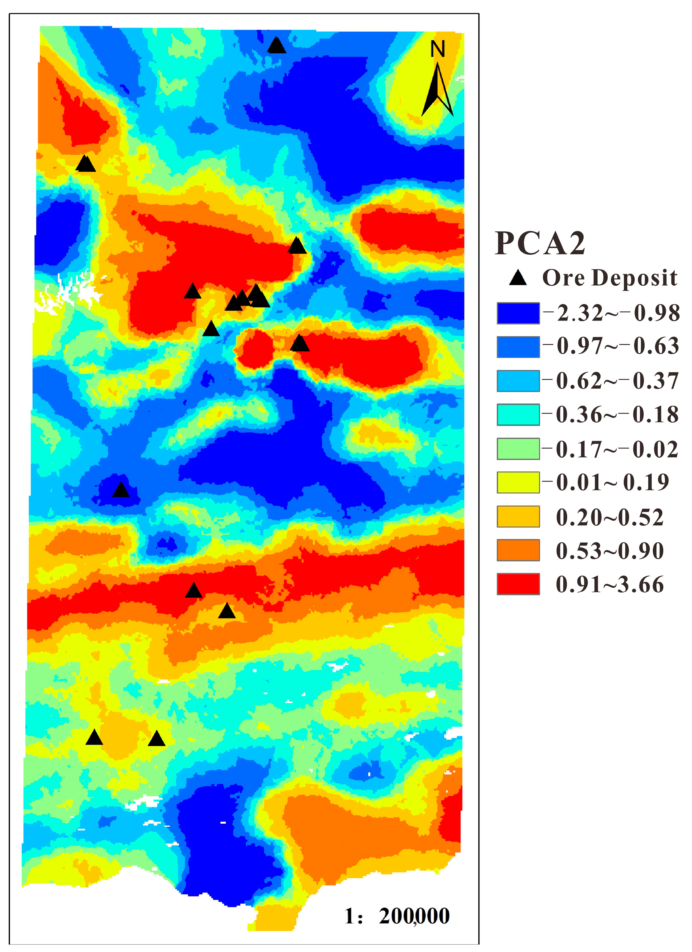
4.2.1. Evidence Layer Information Extraction
- (1)
- Stratum
- (2)
- Regional fracture structure
- (3)
- Regional geochemistry
4.2.2. Establishment of Datasets
4.3. Random Forest Algorithm Implementation
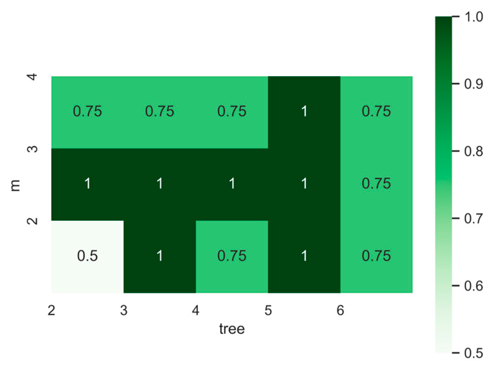
4.3.1. Parameter Optimization
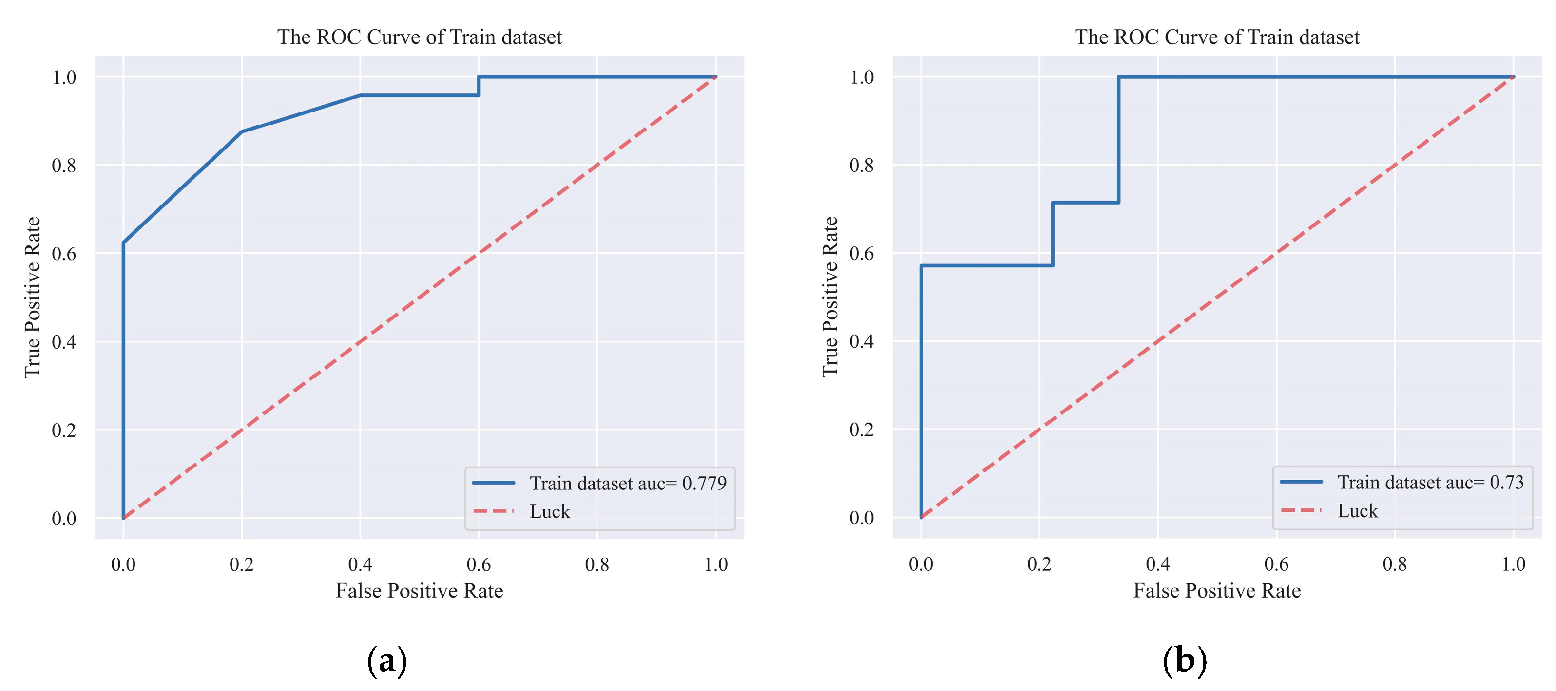
4.3.2. Prediction Performance Assessment
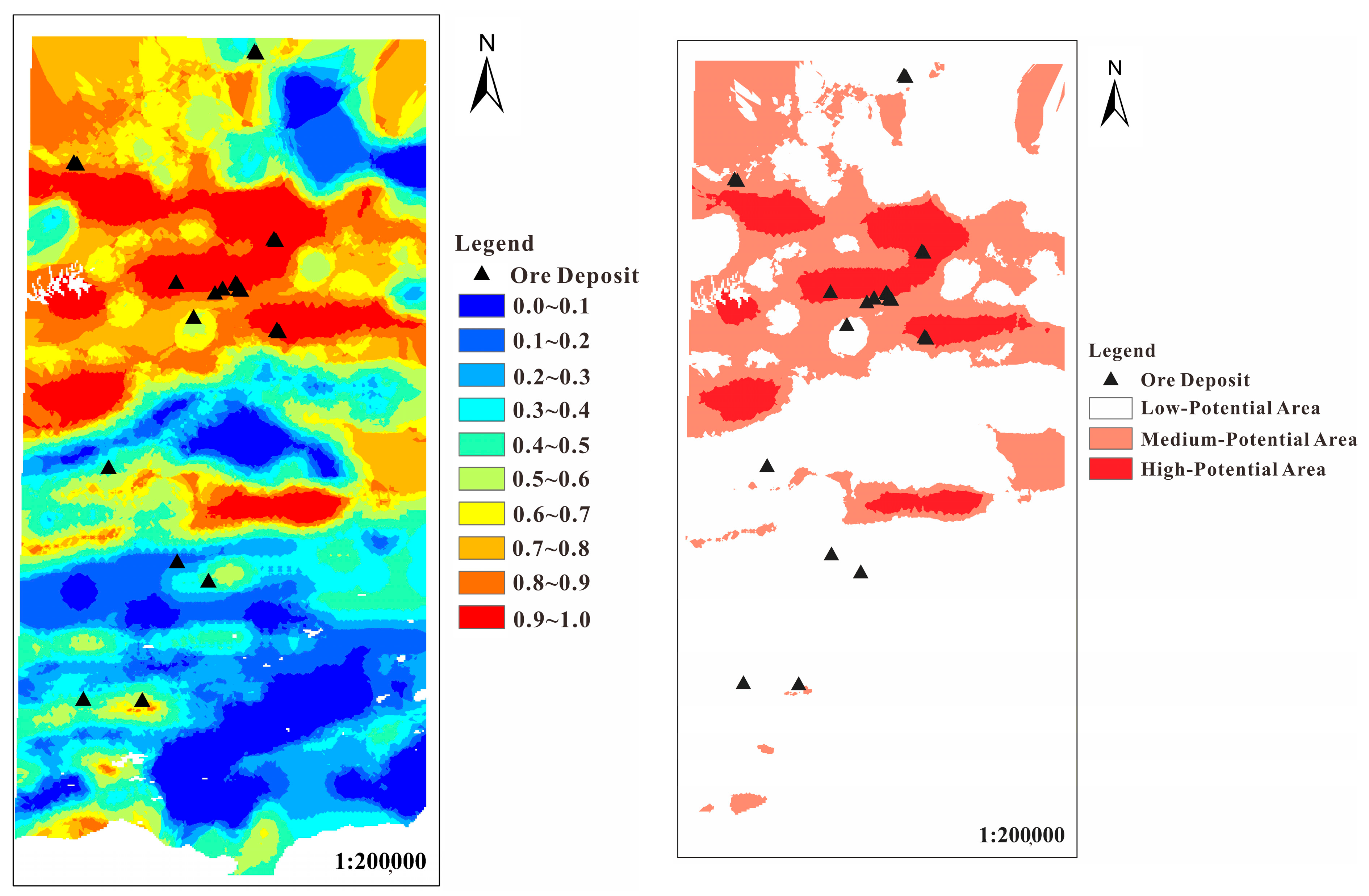
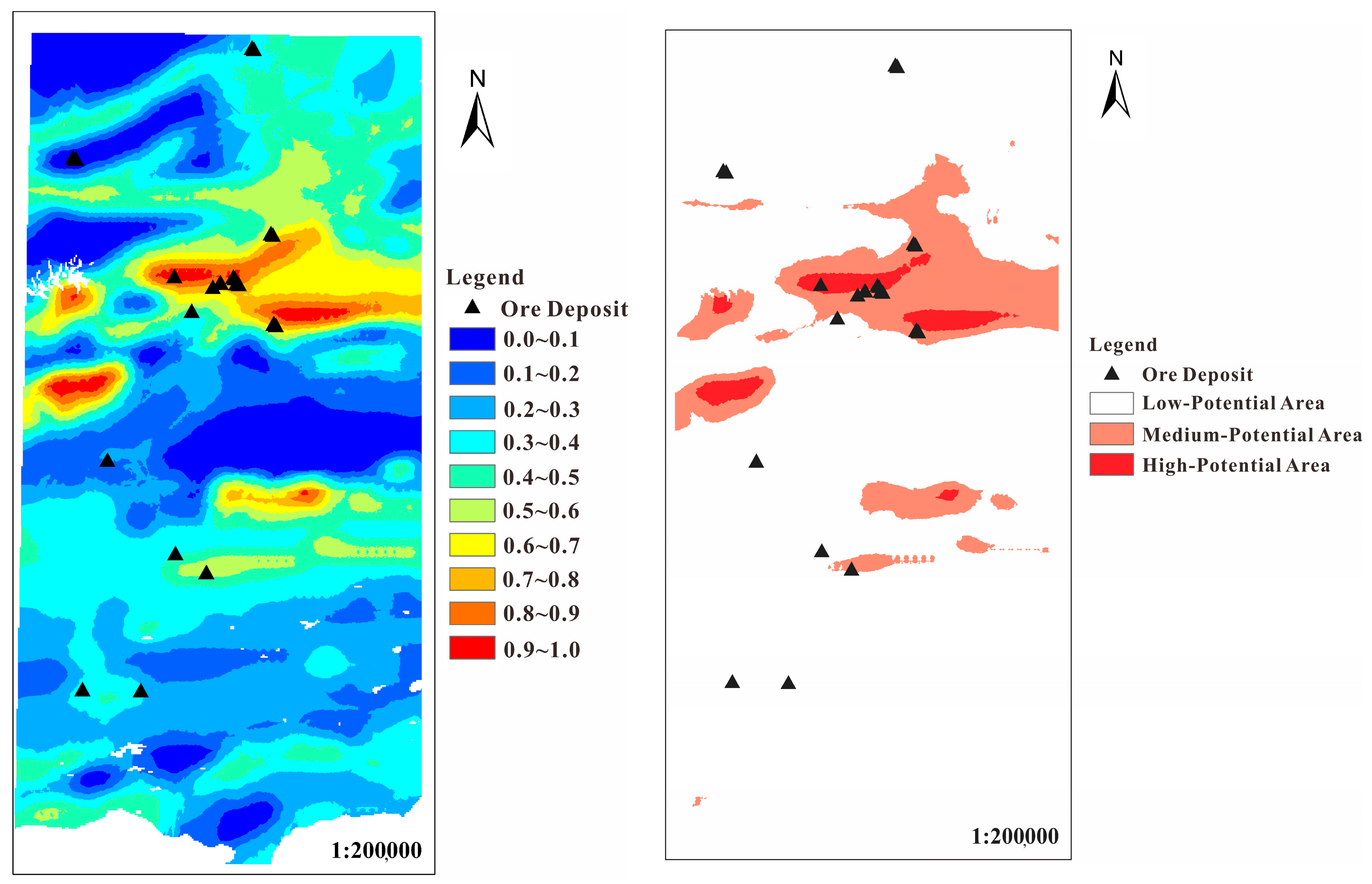
4.3.3. Metallogenic Prediction Results
5. Conclusions
- (1)
- In this study, the strata, fault structure, and geochemical information are extracted, and the known ore spots and geochemical data are used to form a training set and a prediction set to construct a random forest model. The difference between the integrated random undersampling method and the selection of the training sample method is compared, which expands the prospecting idea of machine learning algorithms in mathematical geology in the central Kunlun area of Xinjiang.
- (2)
- For different sampling methods, the performance evaluation parameters of the training process show that the prediction accuracy of the selected training samples is higher, indicating that the fitting effect and generalization ability are stronger. Ensemble random undersampling can weaken the difference between the base learners and achieve consistency in the overall results. The results of metallogenic prospect prediction and potential area division better explain this.
- (3)
- The sampling method of selecting training samples is more reliable because it can fully learn the complex information of the original data, the number of ore spots accurately predicted by the prediction results is greater, and the proportion of ore is higher. For the random forest model of different sampling methods, the random forest algorithm under the selected training samples has more reference value and further exploration significance in the actual exploration problems considering the cost because of its small area of high-potential prediction area and high proportion of ore per unit area.
Author Contributions
Funding
Data Availability Statement
Acknowledgments
Conflicts of Interest
References
- Kong, W.H.; Xiao, K.Y.; Chen, J.P.; Sun, L.; Li, N. A combined prediction method for reducing prediction uncertainty in the quantitative mineral resources prediction. Earth Sci. Front. 2021, 28, 128–138, (In Chinese with English abstract). [Google Scholar] [CrossRef]
- Liu, G.; Wang, Y.Z.; Xue, T.; Wu, C.Y.; Xue, B.; Tang, T.T.; Liu, S.M. Mineral Resource Spatial Association Analysis and Prediction: A Case Study in Western China. Geoscience 2019, 33, 751–758, (In Chinese with English abstract). [Google Scholar] [CrossRef]
- Agterberg, F.; Kelly, A. Geomathematical methods for use in prospecting. Can. Min. J. 1971, 5, 61–72. [Google Scholar]
- Griffiths, J.; Menzie, D.; Labovitz, M. Exploration for and evaluation of natural resources. In Proceedings of the AAPG Research Symposium, Probability Methods in Oil Exploration, Stanford, CA, USA, 20–22 August 1975; pp. 20–22. [Google Scholar]
- Singer, D.A. RESIN, a FORTRAN IV program for determining the area of influence of samples or drill holes in resource target search. Comput. Geosci. 1976, 2, 249–260. [Google Scholar] [CrossRef]
- Singer, D.A. Basic concepts in three-part quantitative assessments of undiscovered mineral resources. Nonrenewable Resour. 1993, 2, 69–81. [Google Scholar] [CrossRef]
- Singer, D.A. Progress in integrated quantitative mineral resource assessments. Ore Geol. Rev. 2010, 3, 242–250. [Google Scholar] [CrossRef]
- Wu, D.C.; Lu, W.Q.; Wang, G.P. 3D geological modeling and metallogenic prediction of Yimaquan M14 magnetic anomaly area in Geermu City of Qinghai. Miner. Resour. Geol. 2023, 37, 55–61, 71, (In Chinese with English abstract). [Google Scholar] [CrossRef]
- Song, W.; Zheng, L.; Liu, J.; Cao, S.; Xie, Z. Genesis, metallogenic model, and prospecting prediction of the Nibao gold deposit in the Guizhou Province, China. Acta Geochim. 2023, 42, 136–152. [Google Scholar] [CrossRef]
- Carranza, E.J.M.; Hale, M. Logistic Regression for Geologically Constrained Mapping of Gold Potential, Baguio District, Philippines. Explor. Min. Geol. 2001, 3, 165–175. [Google Scholar] [CrossRef]
- Li, W.; Neubauer, F.; Liu, Y.J.; Genser, J.; Ren, S.M.; Han, G.Q.; Liang, C.Y. Paleozoic Evolution of the Qimantage Magmatic Arcs, Eastern Kunlun Mountains: Constraints from Zircon Dating of Granitoids and Modern River Sands. J. Asian Earth Sci. 2013, 77, 183–202. [Google Scholar] [CrossRef]
- Seraj, R.R.R. A hybrid GIS-assisted framework to integrate Dempster-Shafer theory of evidence and fuzzy sets in risk analysis: An application in hydrocarbon exploration. Geocarto Int. 2021, 36, 5a8. [Google Scholar] [CrossRef]
- Behera, S.; Panigrahi, M.K. Mineral prospectivity modelling using singularity mapping and multifractal analysis of stream sediment geochemical data from the auriferous Hutti-Maski schist belt, S. India. Ore Geol. Rev. 2021, 131, 104029. [Google Scholar] [CrossRef]
- Koike, K.; Matsuda, S.; Suzuki, T.; Ohmi, M. Neural Network-Based Estimation of Principal Metal Contents in the Hokuroku District, Northern Japan, for Exploring Kuroko-Type Deposits. Nat. Resour. Res. 2002, 2, 135–156. [Google Scholar] [CrossRef]
- Porwal, A.; Carranza, E.J.M.; Hale, M. Artificial Neural Networks for Mineral-Potential Mapping: A Case Study from Aravalli Province, Western India. Nat. Resour. Res. 2003, 3, 155–171. [Google Scholar] [CrossRef]
- Choi, S.; Moon, W.M.; Choi, S.-G. Fuzzy logic fusion of W-Mo exploration data from Seobyeog-ri, Korea. Geosci. J. 2000, 2, 43–52. [Google Scholar] [CrossRef]
- Luo, X.; Dimitrakopoulos, R. Data-driven fuzzy analysis in quantitative mineral resource assessment. Comput. Geosci. 2003, 1, 3–13. [Google Scholar] [CrossRef]
- Liu, Y.; Cheng, Q.M.; Xia, Q.L.; Wang, X.Q. Mineral potential mapping for tungsten polymetallic deposits in the Nanling metallogenic belt, South China. J. Earth Sci. 2014, 4, 689–700. [Google Scholar] [CrossRef]
- Wang, W.L.; Xie, S.Y.; Carranza, E.J.M. Introduction to the thematic collection: Applications of innovations in geochemical data analysis. Geochem. Explor. Environ. Anal. 2022, 23, 1–2. [Google Scholar] [CrossRef]
- Carranza, E.J.M. Weights of Evidence Modeling of Mineral Potential: A Case Study Using Small Number of Prospects, Abra, Philippines. Nat. Resour. Res. 2004, 3, 173–187. [Google Scholar] [CrossRef]
- Yang, F.; Xie, S.Y.; Hao, Z.; Carranza, E.J.M.; Song, Y.; Liu, Q.; Xu, R.; Nie, L.; Han, W.; Wang, C. Geochemical Quantitative Assessment of Mineral Resource Potential in the Da Hinggan Mountains in Inner Mongolia, China. Minerals 2022, 12, 434. [Google Scholar] [CrossRef]
- Brown, W.; Groves, D.; Gedeon, T. Use of Fuzzy Membership Input Layers to Combine Subjective Geological Knowledge and Empirical Data in a Neural Network Method for Mineral-Potential Mapping. Nat. Resour. Res. 2003, 3, 183–200. [Google Scholar] [CrossRef]
- Kim, Y.H.; Choe, K.U.; Ri, R.K. Application of fuzzy logic and geometric average: A Cu sulfide deposits potential mapping case study from Kapsan Basin, DPR Korea. Ore Geol. Rev. 2019, 107, 239–247. [Google Scholar] [CrossRef]
- Xiao, K.Y.; Zhang, X.H.; Song, G.Y.; Chen, Z.H.; Liu, D.L.; Wang, S.L. Development of GIS-Based Mineral Resources Assessment System. Earth Sci. 1999, 5, 525–528, (In Chinese with English abstract). [Google Scholar] [CrossRef]
- Cui, C.Q.; Wang, B.; Zhao, Y.X.; Wang, Q.; Sun, Z.M. China’s regional sustainability assessment on mineral resources: Results from an improved analytic hierarchy process-based normal cloud model. J. Clean. Prod. 2019, 210, 105–120. [Google Scholar] [CrossRef]
- Karapurkar, D.D. RS and GIS based studies on Sediment yield from a tropical watershed: A case study of the Gangolli Catchment, Karnataka. In Proceedings of the Sedimentation, Tectonics, Mineral Resources and Sustainable Development, Hyderabad, India, 7–8 November 2019. [Google Scholar]
- Xie, S.Y.; Wan, X.; Dong, J.B.; Wan, N.; Jiang, X.N.; Carranza, E.J.M.; Wang, X.Q.; Chang, L.H.; Tian, Y. Quantitative Prediction of Potential Areas Likely to Yield Se-rich and Cd-low Rice using Fuzzy Weights-of-Evidence Method. Sci. Total Environ. 2023, 889, 164015. [Google Scholar] [CrossRef] [PubMed]
- Greff, K.; Srivastava, R.K.; Koutnik, J.; Steunebrink, B.R.; Schmidhuber, J. LSTM: A Search Space Odyssey. IEEE Trans. Neural Netw. Learn. Syst. 2017, 10, 2222–2232. [Google Scholar] [CrossRef] [PubMed]
- Agterberg, F. Geomathematics: Theoretical Foundations, Applications and Future Developments; Springer: Cham, Switzerland, 2014; p. 552. [Google Scholar]
- Zhou, Y.Z.; Chen, S.; Zhang, Q.; Xiao, F.; Wang, S.G. Advances and Prospects of Big Data and Mathematical Geoscience. Acta Petrol. Sin. 2018, 2, 255–263. [Google Scholar]
- Rodriguez-Galiano, V.; Sanchez-Castillo, M.; Chica-Olmo, M.; Chica-Rivas, M. Machine Learning Predictive Models for Mineral Prospectivity: An Evaluation of Neural Networks, Random Forest, Regression Trees and Support Vector Machines. Ore Geol. Rev. 2015, 71, 804–818. [Google Scholar] [CrossRef]
- Sun, T.; Chen, F.; Zhong, L.X.; Liu, W.M.; Wang, Y. GIS-based mineral prospectivity mapping using machine learning methods: A case study from Tongling ore district, eastern China. Ore Geol. Rev. 2019, 109, 26–49. [Google Scholar] [CrossRef]
- Nahool, T.A.; Anwar, M.; Yahya, G.A. Utilization of the random forest method for studying some heavy mesons spectra via machine learning technique. Int. J. Mod. Phys. A Part. Fields Gravit. Cosmol. 2022, 37, 2250219. [Google Scholar] [CrossRef]
- Beucher, A.; Siemssen, R.; Fröjdö, S.; Österholm, P.; Martinkauppi, A.; Edén, P. Artificial Neural Network for Mapping and Characterization of Acid Sulfate Soils: Application to Sirppujoki River Catchment, Southwestern Finland. Geoderma 2015, 247–248, 38–50. [Google Scholar] [CrossRef]
- Herrera, M.; Torgo, L.; Izquierdo, J.; Pérez-García, R. Predictive models for forecasting hourly urban water demand. J. Hydrol. 2010, 1–2, 141–150. [Google Scholar] [CrossRef]
- Xie, S.Y.; Huang, N.; Deng, J.; Wu, S.L.; Zhan, M.G.; Carranza, E.J.M.; Zhang, Y.P.; Meng, F.X. Quantitative Prediction of Prospectivity for Pb–Zn Deposits in Guangxi (China) by Back-propagation Neural Network and Fuzzy Weights-of-Evidence Modeling. Geochem. Explor. Environ. Anal. 2022, 22, 1–10. [Google Scholar] [CrossRef]
- Rodriguez-Galiano, V.F.; Ghimire, B.; Rogan, J.; Chica-Olmo, M.; Rigol-Sanchez, J.P. An assessment of the effectiveness of a random forest classifier for land-cover classification. ISPRS J. Photogramm. Remote Sens. 2012, 67, 93–104. [Google Scholar] [CrossRef]
- Dong, L.H.; Zhang, L.C.; Li, W.D. Division and characteristics of geotectonic units in Xinjiang. In Proceedings of the 6th Tianshan Geological and Mineral Resources Symposium, Urumqi, China, 1 January 2008; pp. 25–32. (In Chinese). [Google Scholar]
- Pan, Y.S. Formation and Uplifting of the QingHai-Tibet Plateau. Earth Sci. Front. 1999, 3, 153–163, (In Chinese with English abstract). [Google Scholar] [CrossRef]
- Liu, C.Y.; Liu, T. Discovery and Significance of Porphyritic Copper Mineralization in YunwuNing of XinJiang. Xinjiang Geol. 1998, 2, 185–187, (In Chinese with English abstract). [Google Scholar]
- Zhang, Y.P.; Ye, X.F.; Xie, S.Y.; Zhou, X.Y.; Awadelseid, S.F.; Yaisamut, O.; Meng, F.X. Implication of multifractal analysis for quantitative evaluation of mineral resources in the Central Kunlun area, Xinjiang, China. Geochem. Explor. Environ. Anal. 2022, 22, geochem2021-083. [Google Scholar] [CrossRef]
- Breiman, L. Random forests. Mach. Learn. 2001, 1, 5–32. [Google Scholar] [CrossRef]
- Martins, T.F.; Seoane, J.C.S.; Tavares, F.M. Cu-Au exploration target generation in the eastern Carajás Mineral Province using random forest and multi-class index overlay mapping. J. S. Am. Earth Sci. 2022, 116, 103790. [Google Scholar] [CrossRef]
- Oshiro, T.M.; Perez, P.S.; Baranauskas, J.A. How Many Trees in a Random Forest ? In Machine Learning and Data Mining in Pattern Recognition; Springer: Berlin/Heidelberg, Germany, 2012; pp. 154–168. [Google Scholar]
- Liu, T.Y. EasyEnsemble and Feature Selection for Imbalance Data Sets. In Proceedings of the 2009 International Joint Conference on Bioinformatics, Systems Biology and Intelligent Computing, Shanghai, China, 3–5 August 2009; pp. 517–520. [Google Scholar]
- Xiong, Y.; Zuo, R. Effects of misclassification costs on mapping mineral prospectivity. Ore Geol. Rev. 2017, 82, 1–9. [Google Scholar] [CrossRef]
- Feng, K.; Hong, H.; Tang, K.; Wang, J. Decision making with machine learning and roc curves. arXiv 2019, arXiv:1905.02810v1. [Google Scholar] [CrossRef]
- Kim, E.; Kim, W.; Lee, Y. Combination of multiple classifiers for the customer’s purchase behavior prediction. Decis. Support Syst. 2003, 2, 167–175. [Google Scholar] [CrossRef]
- Cui, X.L.; Liu, T.T.; Wang, W.H.; Jing, M.; Bai, Y. Characteristics of geochemistry and prospecting direction of stream sediments in Buqingshan area, East Kunlun Mountains. Geophys. Geochem. Explor. 2011, 35, 573–578, (In Chinese with English abstract). [Google Scholar]
- Guo, Y.; Gong, F.Z.; Ning, J.S.; Liu, Y.C.; Liu, Z. Comparative study of the content area fractal method and the traditional statistical method for determining the anomaly lower limit: A case study of Au element of stream sediment survey in Awengcuo area of Tibet. Miner. Resour. Geol. 2018, 4, 736–741, (In Chinese with English abstract). [Google Scholar]
- Thanh, T.N.; Tuyen, D.V. Identification of Multivariate Geochemical Anomalies Using Spatial Autocorrelation Analysis and Robust Statistics. Ore Geol. Rev. 2019, 111, 102985. [Google Scholar] [CrossRef]
- Feng, C.Y.; Wang, S.; Li, G.C.; Ma, S.C.; Li, D.S. Middle to Late Triassic granitoids in the Qimantage area, Qinghai Province, China: Chronology, geochemistry and metallogenic significances. Acta Petrol. Sin. 2012, 28, 665–678, (In Chinese with English abstract). [Google Scholar]
- Guo, Z.F.; Deng, J.F.; Xu, Z.Q.; Mo, X.X.; Luo, Z.H. Late Palaeozoic-Mesozoic Intracontinental, Orogenic Process and Inter Medate-Acidic Igneous Rocks from the Eastern KunLun Mountains of NorthWestern China. Geoscience 1998, 3, 51–59, (In Chinese with English abstract). [Google Scholar]
- Zheng, M.T.; Zhang, L.C.; Zhu, M.T.; Li, Z.Q.; He, L.D.; Shi, Y.J.; Dong, L.H.; Feng, J. Geological characteristics, formation age and genesis of the Kalaizi Ba-Fe deposit in West Kunlun. Earth Sci. Front. 2016, 5, 252–265, (In Chinese with English abstract). [Google Scholar] [CrossRef]
- Omar, L.; Ivrissimtzis, I. Using theoretical ROC curves for analysing machine learning binary classifiers. Pattern Recognit. Lett. 2019, 128, 447–451. [Google Scholar] [CrossRef]


| Predicted Positive (PP) | Predicted Negative (PN) | |
|---|---|---|
| Actual Positive (AP) | TP (True Positive) | FN (False Negative) |
| Actual Negative (AN) | FP (False Positive) | TN (True Negative) |
| Geological Unit | N | E | K | J | T | P | C | Ch | Whole Area | |
|---|---|---|---|---|---|---|---|---|---|---|
| Parameter | ||||||||||
| Au | Mean Value | 1.0 | 1.1 | 0.6 | 0.7 | 0.8 | 1.1 | 1.6 | 2.1 | 1.1 |
| Standard Deviation | 0.8 | 1.2 | 0.4 | 0.7 | 0.6 | 2.2 | 1.6 | 2.8 | 1.5 | |
| Coefficient of Variation | 0.8 | 1.1 | 0.7 | 0.9 | 0.8 | 2.0 | 1.0 | 1.2 | 1.4 | |
| Concentration Coefficient | 0.9 | 1.0 | 0.5 | 0.7 | 0.7 | 1.0 | 1.4 | 1.9 | 1.0 | |
| Ba | Mean Value | 639.6 | 756.5 | 677.9 | 1598.3 | 793.9 | 580.1 | 526.3 | 513.9 | 766.7 |
| Standard Deviation | 502.1 | 531.1 | 130.1 | 6135.3 | 1776.1 | 326.5 | 219.6 | 95.3 | 2307.8 | |
| Coefficient of Variation | 0.8 | 0.7 | 0.2 | 3.8 | 2.2 | 0.5 | 0.4 | 0.1 | 3.0 | |
| Concentration Coefficient | 0.8 | 1.0 | 0.9 | 2.0 | 1.0 | 0.7 | 0.6 | 0.6 | 1.0 | |
| Bi | Mean Value | 0.3 | 0.2 | 0.2 | 0.2 | 0.2 | 0.2 | 0.2 | 0.2 | 0.2 |
| Standard Deviation | 0.4 | 0.1 | 0.1 | 0.1 | 0.1 | 0.1 | 0.1 | 0.1 | 0.2 | |
| Coefficient of Variation | 1.1 | 0.5 | 0.2 | 0.5 | 0.3 | 0.7 | 0.5 | 0.4 | 1.0 | |
| Concentration Coefficient | 1.5 | 1.0 | 0.5 | 1.0 | 1.0 | 1.0 | 1.0 | 1.0 | 1.0 | |
| Co | Mean Value | 11.6 | 9.7 | 7.6 | 8.9 | 12.1 | 10.7 | 10.1 | 7.8 | 10.7 |
| Standard Deviation | 3.0 | 4.5 | 2.2 | 3.9 | 3.1 | 3.6 | 3.6 | 3.3 | 4.3 | |
| Coefficient of Variation | 0.3 | 0.5 | 0.3 | 0.4 | 0.2 | 0.3 | 0.3 | 0.4 | 0.4 | |
| Concentration Coefficient | 1.1 | 0.9 | 0.7 | 0.8 | 1.1 | 0.9 | 0.9 | 0.7 | 1.0 | |
| Cu | Mean Value | 21.5 | 21.5 | 18.7 | 25.2 | 26.6 | 20.7 | 27.6 | 28.2 | 24.4 |
| Standard Deviation | 4.9 | 9.8 | 3.8 | 9.9 | 8.9 | 7.4 | 16.6 | 22.7 | 11.1 | |
| Coefficient of Variation | 0.2 | 0.5 | 0.2 | 0.3 | 0.3 | 0.3 | 0.6 | 0.7 | 0.4 | |
| Concentration Coefficient | 0.9 | 0.9 | 0.8 | 1.0 | 1.1 | 0.8 | 1.1 | 1.1 | 1.0 | |
| Fe | Mean Value | 4.7 | 3.7 | 3.1 | 4.3 | 5.2 | 4.4 | 4.0 | 3.1 | 4.4 |
| Standard Deviation | 1.2 | 1.7 | 0.7 | 1.8 | 1.4 | 1.4 | 1.3 | 1.0 | 1.7 | |
| Coefficient of Variation | 0.3 | 0.5 | 0.2 | 0.4 | 0.2 | 0.3 | 0.3 | 0.3 | 0.4 | |
| Concentration Coefficient | 1.1 | 0.8 | 0.7 | 0.9 | 1.1 | 1.0 | 0.9 | 0.7 | 1.0 | |
| Mg | Mean Value | 1.3 | 1.6 | 1.2 | 1.4 | 1.7 | 1.6 | 2.0 | 1.6 | 1.7 |
| Standard Deviation | 0.4 | 0.8 | 0.4 | 0.6 | 0.3 | 0.4 | 0.7 | 1.0 | 0.8 | |
| Coefficient of Variation | 0.3 | 0.5 | 0.3 | 0.4 | 0.2 | 0.3 | 0.3 | 0.6 | 0.5 | |
| Concentration Coefficient | 0.8 | 0.9 | 0.7 | 0.8 | 1.0 | 0.9 | 1.1 | 0.9 | 1.0 | |
| Sn | Mean Value | 2.7 | 1.8 | 1.4 | 1.7 | 2.1 | 2.1 | 2.1 | 2.9 | 2.3 |
| Standard Deviation | 1.3 | 0.8 | 0.2 | 0.5 | 0.8 | 1.0 | 0.7 | 1.0 | 2.0 | |
| Coefficient of Variation | 0.5 | 0.4 | 0.1 | 0.3 | 0.4 | 0.4 | 0.3 | 0.3 | 0.9 | |
| Concentration Coefficient | 1.2 | 0.8 | 0.6 | 0.7 | 0.9 | 0.9 | 0.9 | 1.2 | 1.0 | |
| Ti | Mean Value | 3160.2 | 2395.3 | 1861.3 | 1880.9 | 2805.9 | 2515.4 | 2509.1 | 2244.3 | 2574.3 |
| Standard Deviation | 1840.7 | 979.1 | 676.5 | 875.1 | 939.3 | 967.3 | 795.5 | 631.9 | 1162.0 | |
| Coefficient of Variation | 0.5 | 0.4 | 0.3 | 0.4 | 0.3 | 0.4 | 0.3 | 0.3 | 0.4 | |
| Concentration Coefficient | 1.2 | 0.9 | 0.7 | 0.7 | 1.0 | 1.0 | 1.0 | 0.9 | 1.0 | |
| V | Mean Value | 65.4 | 60.8 | 53.4 | 49.5 | 64.0 | 59.3 | 71.1 | 55.0 | 63.1 |
| Standard Deviation | 19.8 | 25.4 | 22.1 | 18.2 | 17.5 | 22.7 | 26.2 | 32.9 | 25.8 | |
| Coefficient of Variation | 0.3 | 0.4 | 0.4 | 0.3 | 0.2 | 0.4 | 0.3 | 0.6 | 0.4 | |
| Concentration Coefficient | 1.0 | 0.9 | 0.8 | 0.7 | 1.0 | 0.9 | 1.1 | 0.9 | 1.0 | |
| Pb | Mean Value | 20.5 | 15.2 | 14.8 | 17.6 | 21.8 | 19.2 | 15.3 | 15.6 | 18.4 |
| Standard Deviation | 5.6 | 21.3 | 3.4 | 13.5 | 21.9 | 7.6 | 5.4 | 3.2 | 15.1 | |
| Coefficient of Variation | 0.3 | 1.4 | 0.2 | 0.7 | 1.0 | 0.4 | 0.3 | 0.2 | 0.8 | |
| Concentration Coefficient | 1.1 | 0.8 | 0.8 | 0.9 | 1.1 | 1.0 | 0.8 | 0.8 | 1.0 | |
| Zn | Mean Value | 68.9 | 50.1 | 46.1 | 64.6 | 78.3 | 65.5 | 64.8 | 60.0 | 66.0 |
| Standard Deviation | 18.2 | 22.7 | 11.9 | 79.3 | 65.0 | 25.6 | 21.5 | 24.1 | 48.6 | |
| Coefficient of Variation | 0.3 | 0.4 | 0.2 | 1.2 | 0.8 | 0.4 | 0.3 | 0.4 | 0.7 | |
| Concentration Coefficient | 1.0 | 0.7 | 0.7 | 0.9 | 1.1 | 1.0 | 0.9 | 0.9 | 1.0 |
| Component | Initial Eigenvalues | Rotation Sums of Squared Loadings | ||||
|---|---|---|---|---|---|---|
| Total | % of Variance | Cumulative % | Total | % of Variance | Cumulative % | |
| 1 | 4.65 | 38.75 | 38.75 | 4.31 | 35.91 | 35.91 |
| 2 | 1.85 | 15.44 | 54.19 | 1.95 | 16.23 | 52.14 |
| 3 | 1.56 | 13.01 | 67.19 | 1.80 | 15.00 | 67.14 |
| 4 | 1.01 | 8.39 | 75.58 | 1.01 | 8.44 | 75.58 |
| 5 | 0.92 | 7.67 | 83.25 | |||
| 6 | 0.64 | 5.35 | 88.60 | |||
| 7 | 0.43 | 3.61 | 92.21 | |||
| 8 | 0.33 | 2.76 | 94.96 | |||
| 9 | 0.27 | 2.21 | 97.18 | |||
| 10 | 0.19 | 1.58 | 98.75 | |||
| 11 | 0.10 | 0.81 | 99.56 | |||
| 12 | 0.05 | 0.44 | 100.00 | |||
| RF | |
|---|---|
| Min | 0.50 |
| Max | 1.00 |
| Mean | 0.85 |
| Std | 0.16 |
| Select Training Samples | Integrated Random Undersampling | |
|---|---|---|
| RF | RF | |
| Acc | 1.00 | 0.75 |
| Acc+ | 1.00 | 1.00 |
| Acc- | 1.00 | 0.60 |
| G-mean | 1.00 | 0.87 |
| Integrated Random Undersampling | Select Training Samples | ||
|---|---|---|---|
| RF | RF | ||
| Low-potential areas | Known number of occurrence | 7 | 5 |
| Area (km2) | 11,240 | 13,768 | |
| Ore-bearing ratio (%) | 0.062 | 0.036 | |
| Mineralization potential area | Known number of occurrence | 9 | 10 |
| Area (km2) | 3447 | 1702 | |
| Ore-bearing ratio (%) | 0.261 | 0.588 | |
| High-potential areas | Known number of occurrence | 11 | 12 |
| Area (km2) | 1068 | 286 | |
| Ore-bearing ratio (%) | 1.030 | 4.196 | |
Disclaimer/Publisher’s Note: The statements, opinions and data contained in all publications are solely those of the individual author(s) and contributor(s) and not of MDPI and/or the editor(s). MDPI and/or the editor(s) disclaim responsibility for any injury to people or property resulting from any ideas, methods, instructions or products referred to in the content. |
© 2023 by the authors. Licensee MDPI, Basel, Switzerland. This article is an open access article distributed under the terms and conditions of the Creative Commons Attribution (CC BY) license (https://creativecommons.org/licenses/by/4.0/).
Share and Cite
Zhang, Y.; Ye, X.; Xie, S.; Dong, J.; Yaisamut, O.; Zhou, X.; Zhou, X. Prediction of Au-Polymetallic Deposits Based on Spatial Multi-Layer Information Fusion by Random Forest Model in the Central Kunlun Area of Xinjiang, China. Minerals 2023, 13, 1302. https://doi.org/10.3390/min13101302
Zhang Y, Ye X, Xie S, Dong J, Yaisamut O, Zhou X, Zhou X. Prediction of Au-Polymetallic Deposits Based on Spatial Multi-Layer Information Fusion by Random Forest Model in the Central Kunlun Area of Xinjiang, China. Minerals. 2023; 13(10):1302. https://doi.org/10.3390/min13101302
Chicago/Turabian StyleZhang, Yuepeng, Xiaofeng Ye, Shuyun Xie, Jianbiao Dong, Oraphan Yaisamut, Xuwei Zhou, and Xiaoying Zhou. 2023. "Prediction of Au-Polymetallic Deposits Based on Spatial Multi-Layer Information Fusion by Random Forest Model in the Central Kunlun Area of Xinjiang, China" Minerals 13, no. 10: 1302. https://doi.org/10.3390/min13101302