
Orebody Modeling Method Based on the Coons Surface Interpolation

 ,
,
Abstract
:1. Introduction
1.1. Related Research Work
1.1.1. Free-Form Surface Reconstruction
1.1.2. Contour Interpolation Modeling
1.1.3. Orebody Modeling
1.2. Solution Strategy
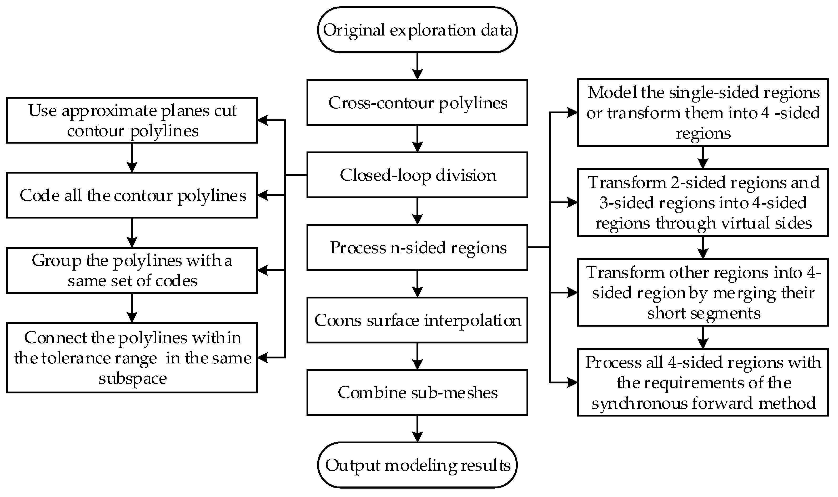
2. Overview of the Method
- Use approximate planes of each contour polyline to cut all polylines for the closed-loop division.
- Preprocess the formed loops and separately model the processed four-sided regions through Coons surface interpolation.
- Combine all the sub-meshes to construct a complete orebody model.
3. Method
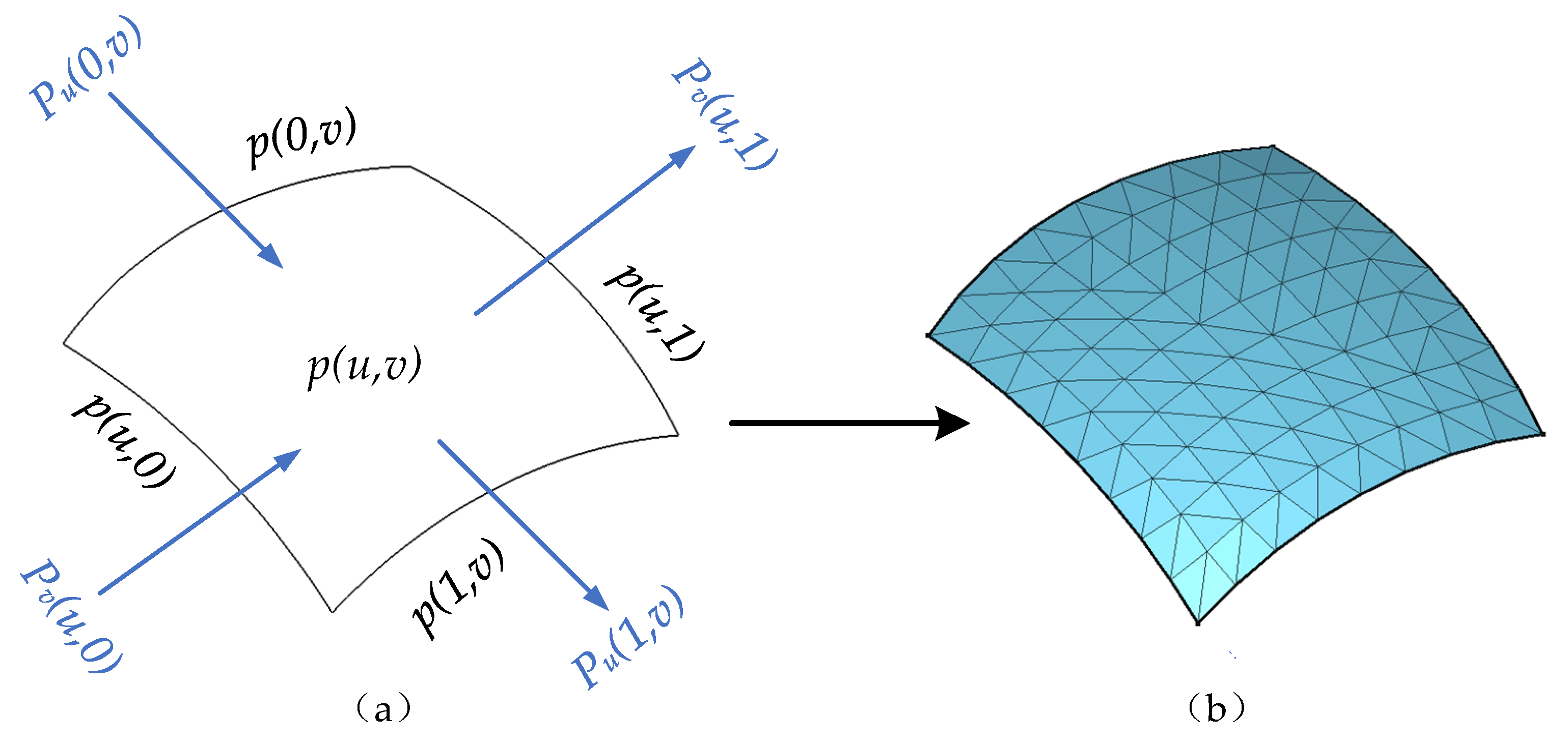
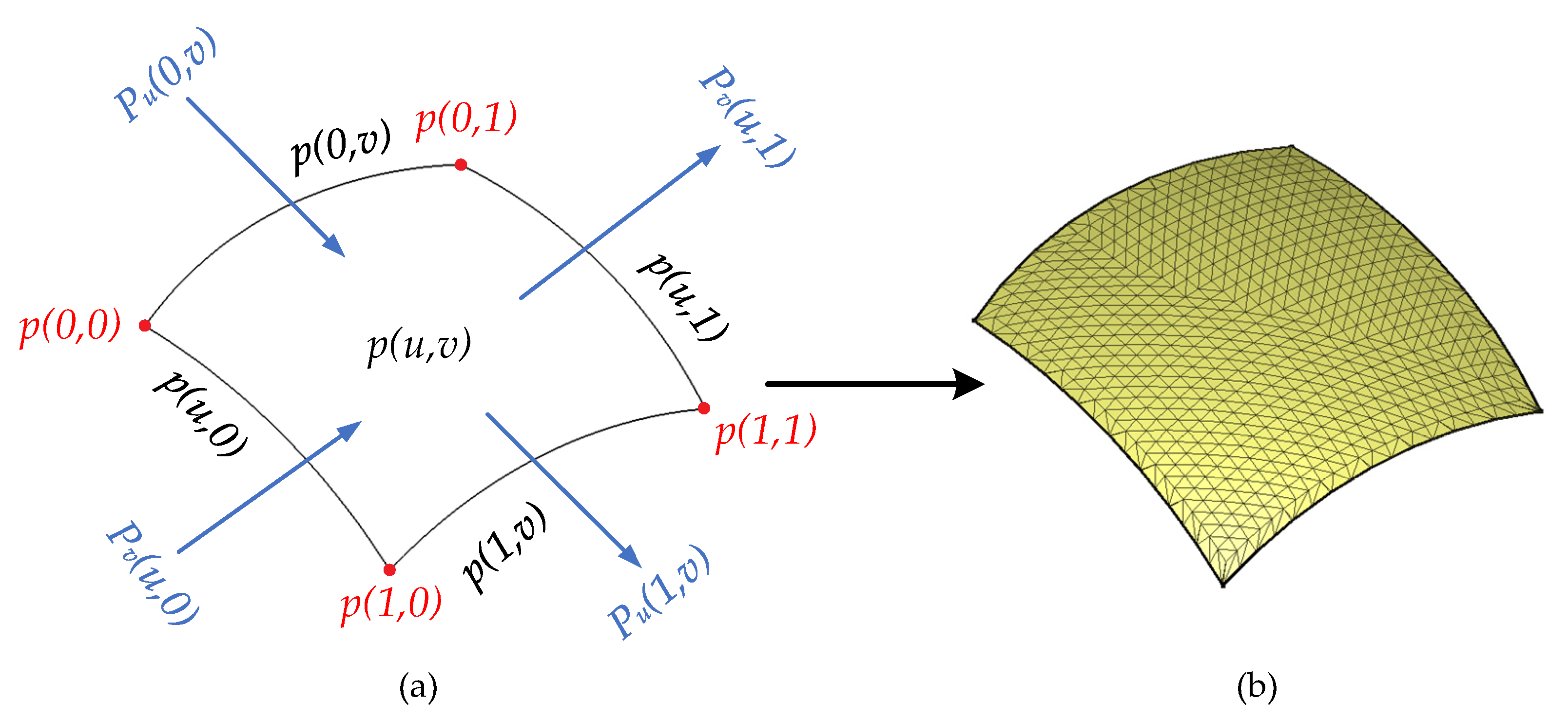
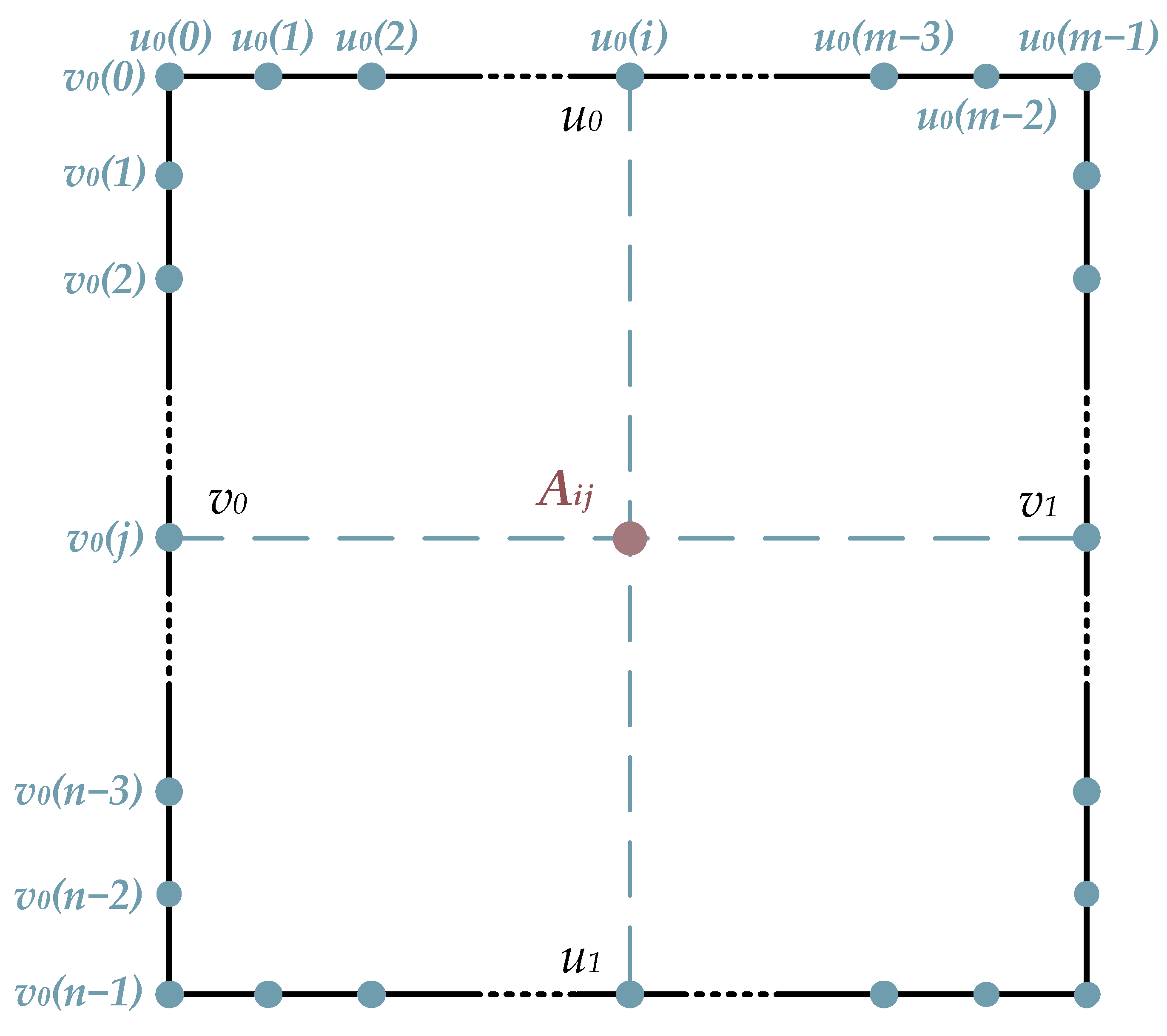
3.1. Coons Surface
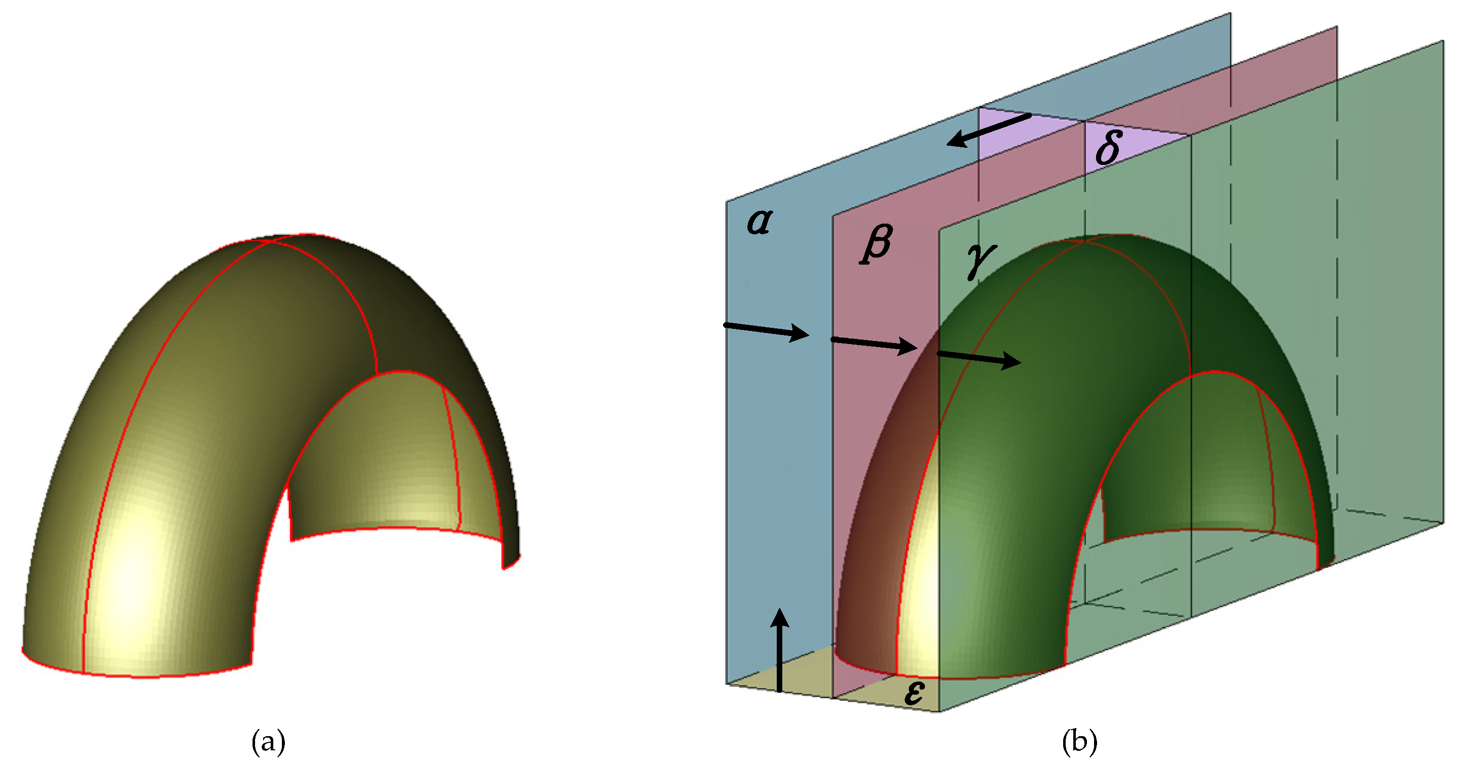
3.2. Closed-Loop Division
3.3. Process n-Sided Regions
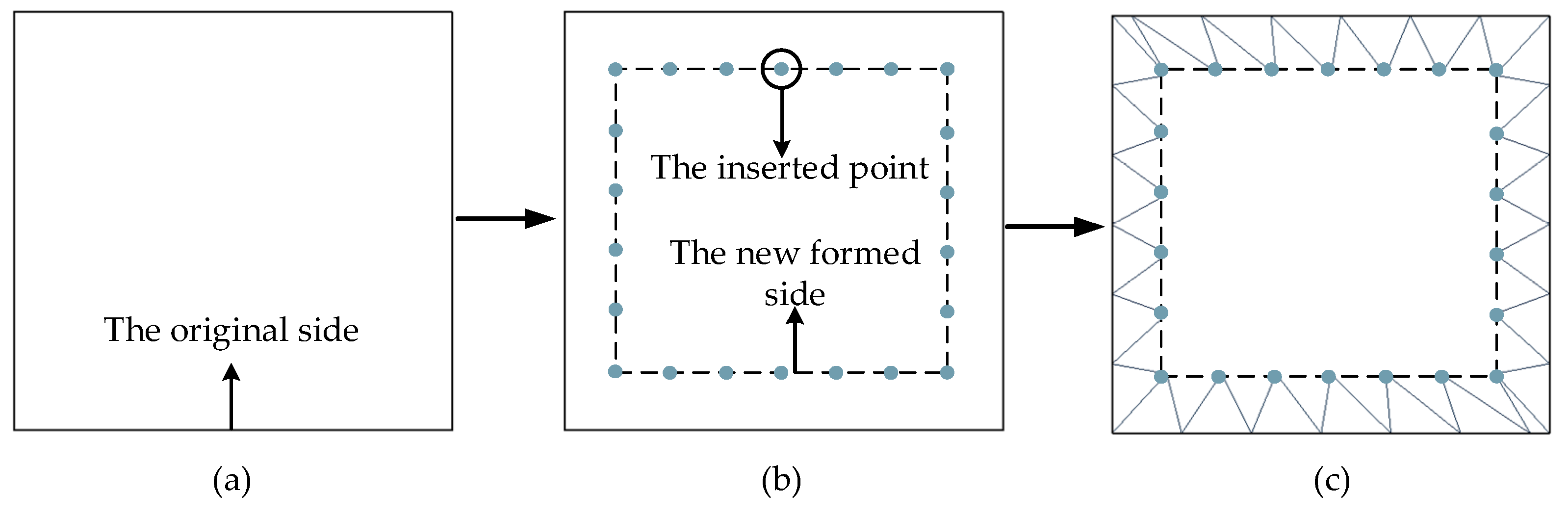
3.3.1. Process the Single-Sided Region
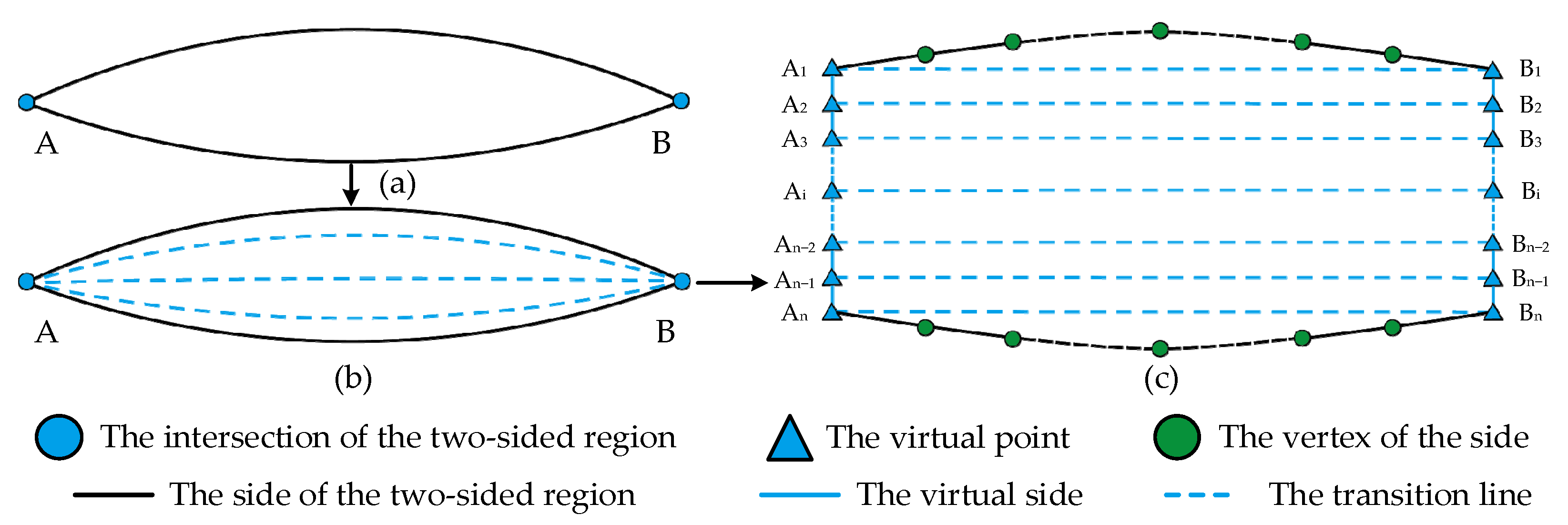
3.3.2. Process the Two-Sided and the Three-Sided Regions
3.3.3. Process Other Regions
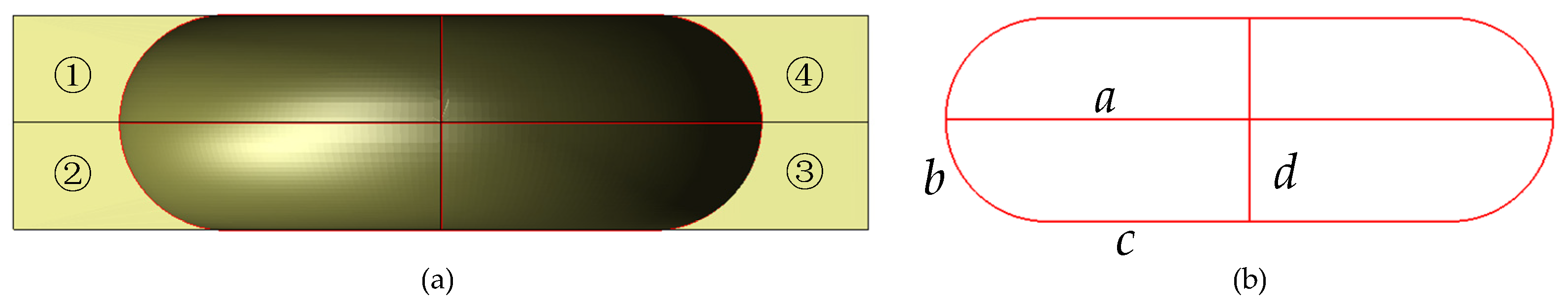
3.3.4. Process All the Four-Sided Regions
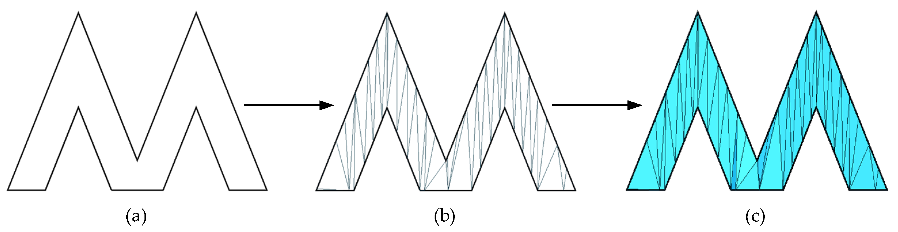
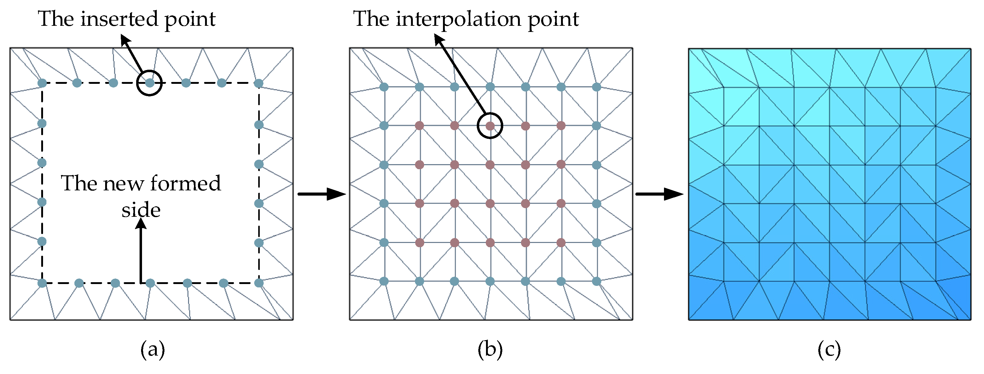
3.4. Sided Region Modeling
3.5. Combine Sub-Meshes
4. Results and Discussion
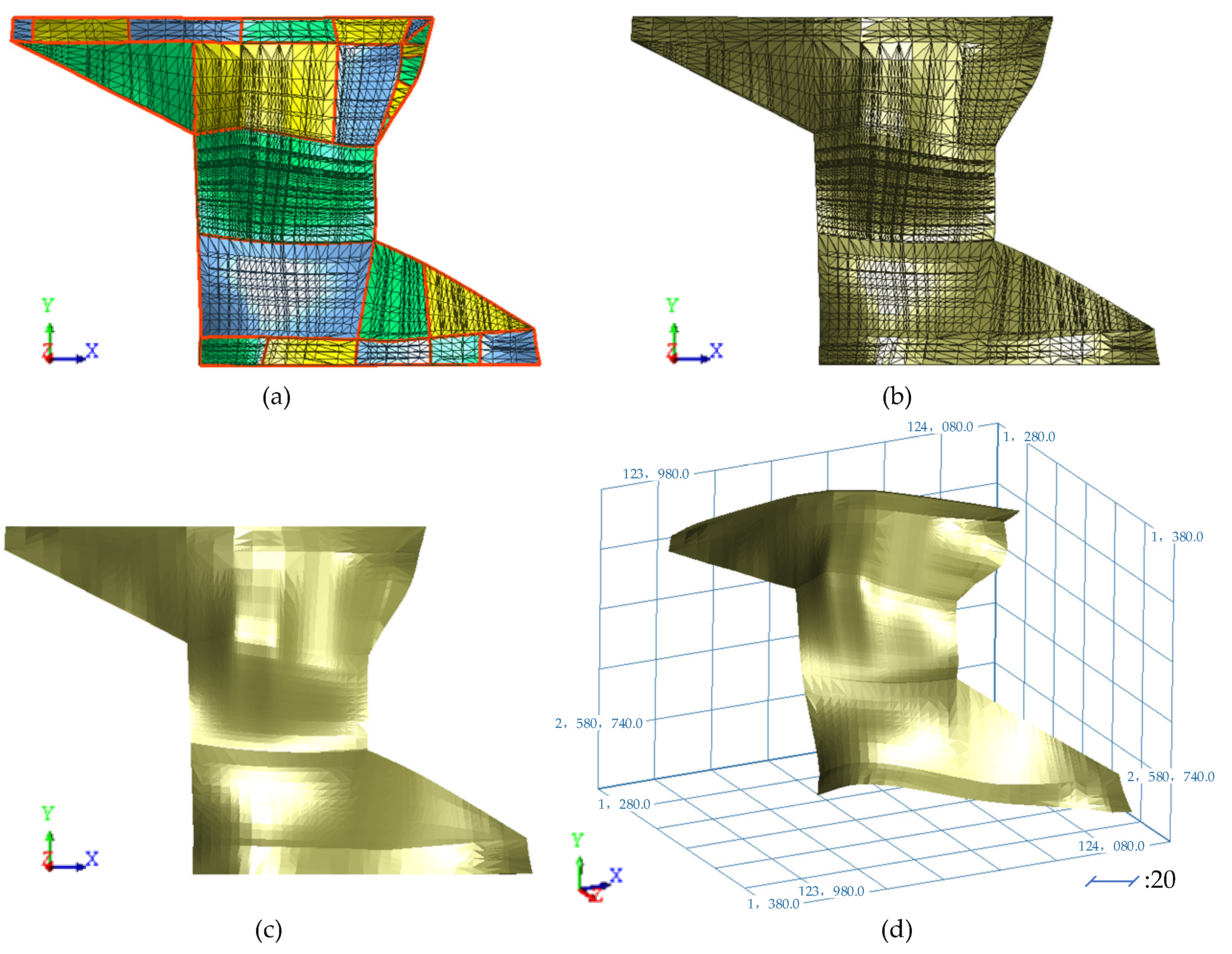
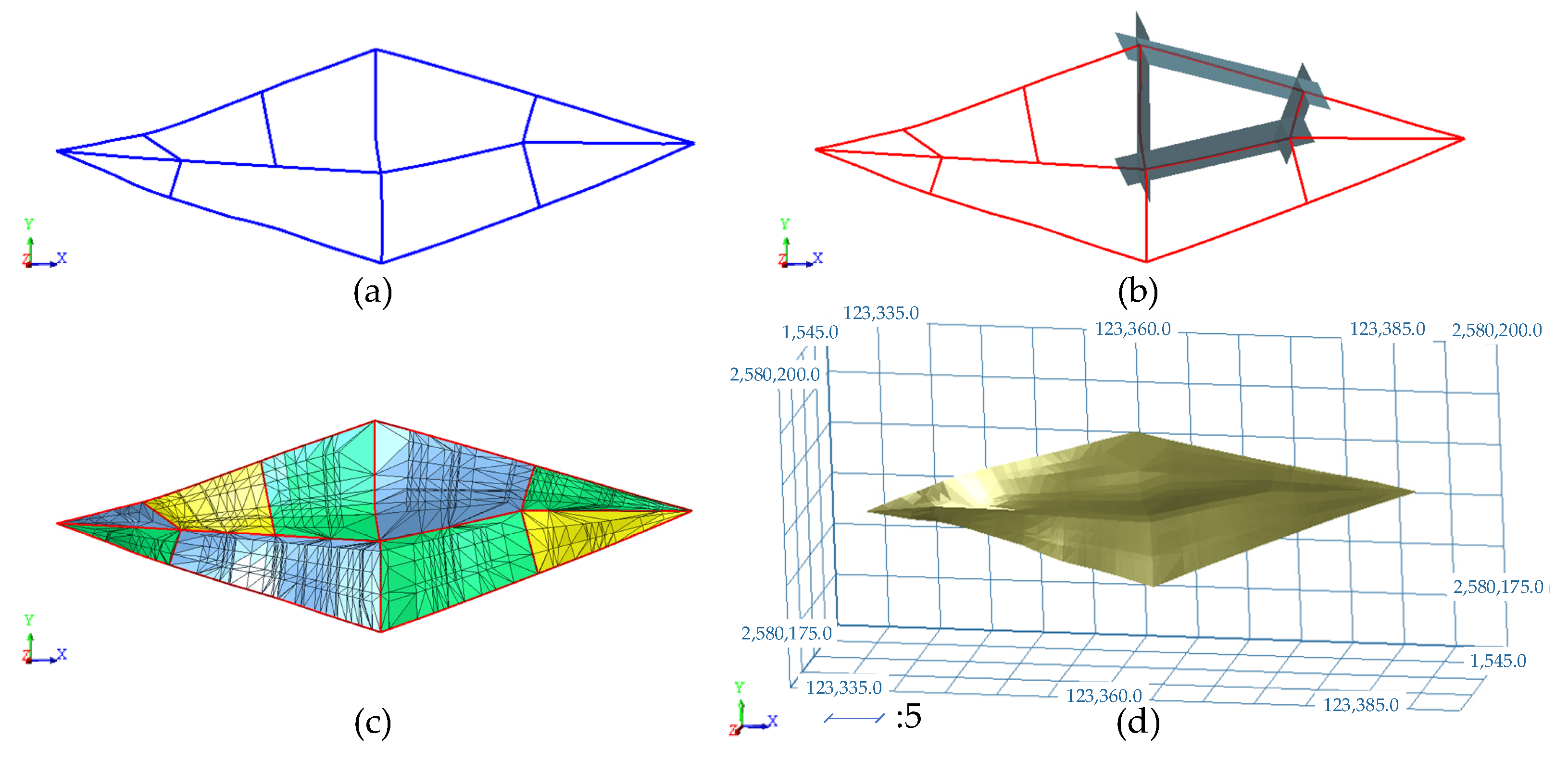
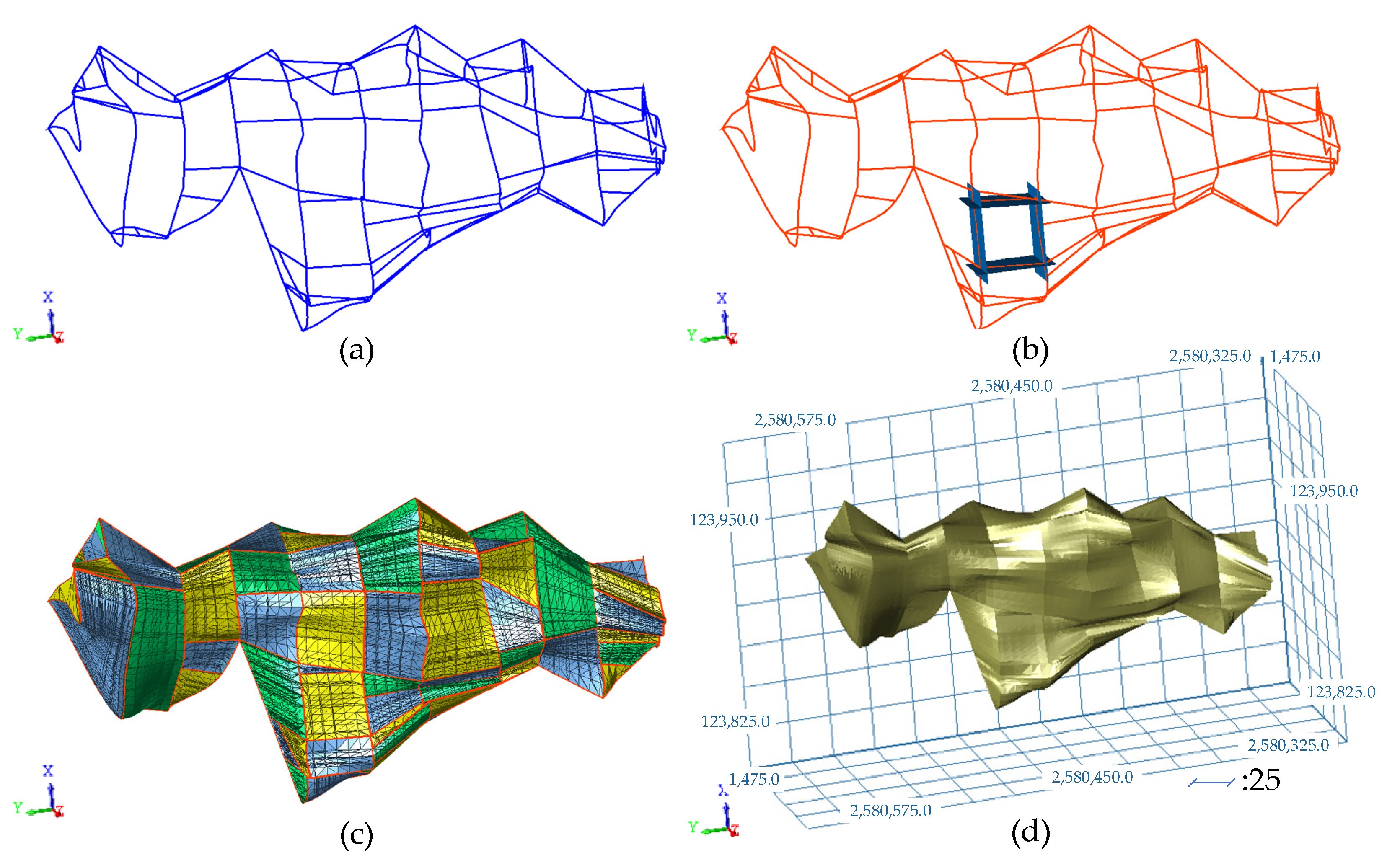
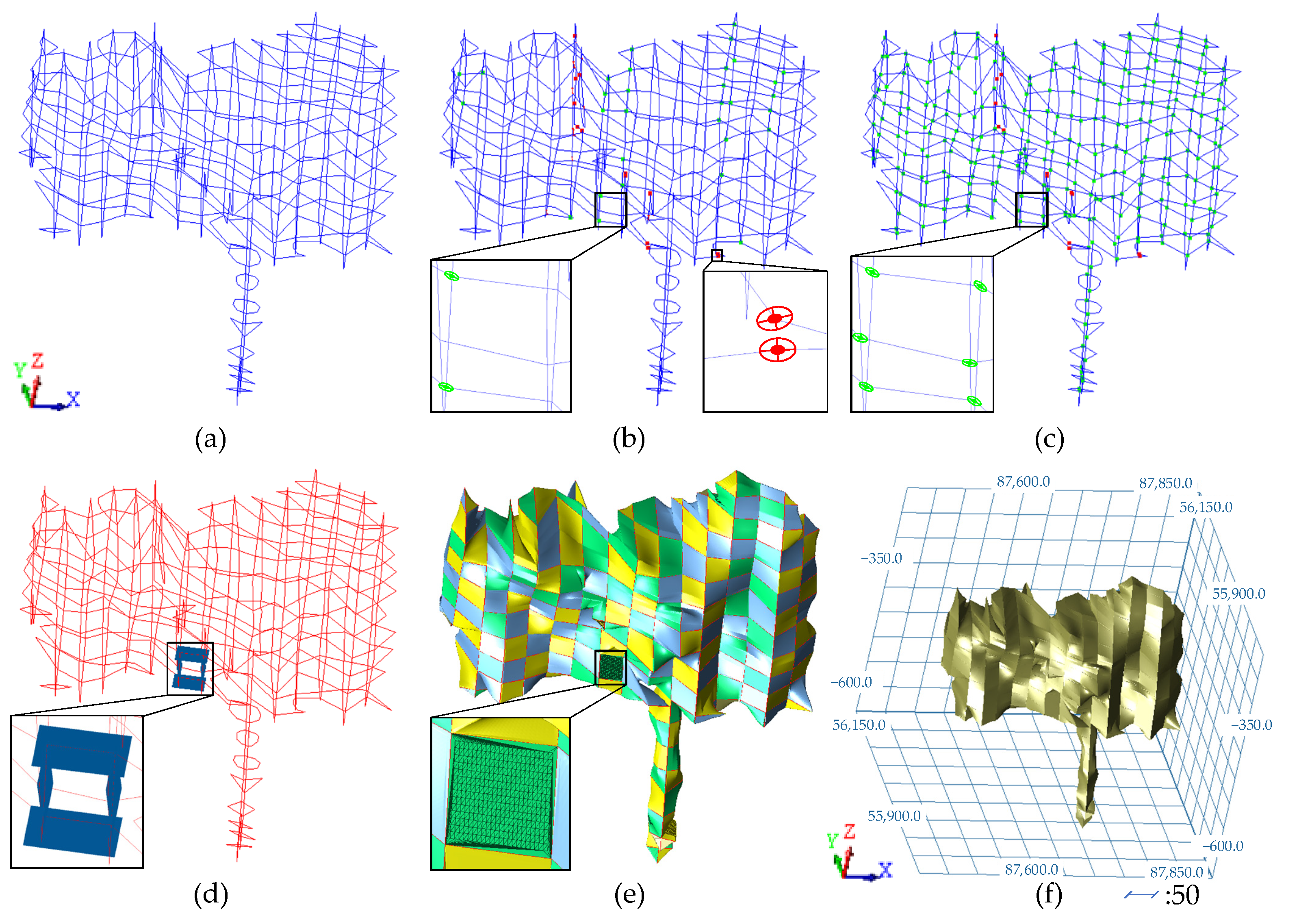
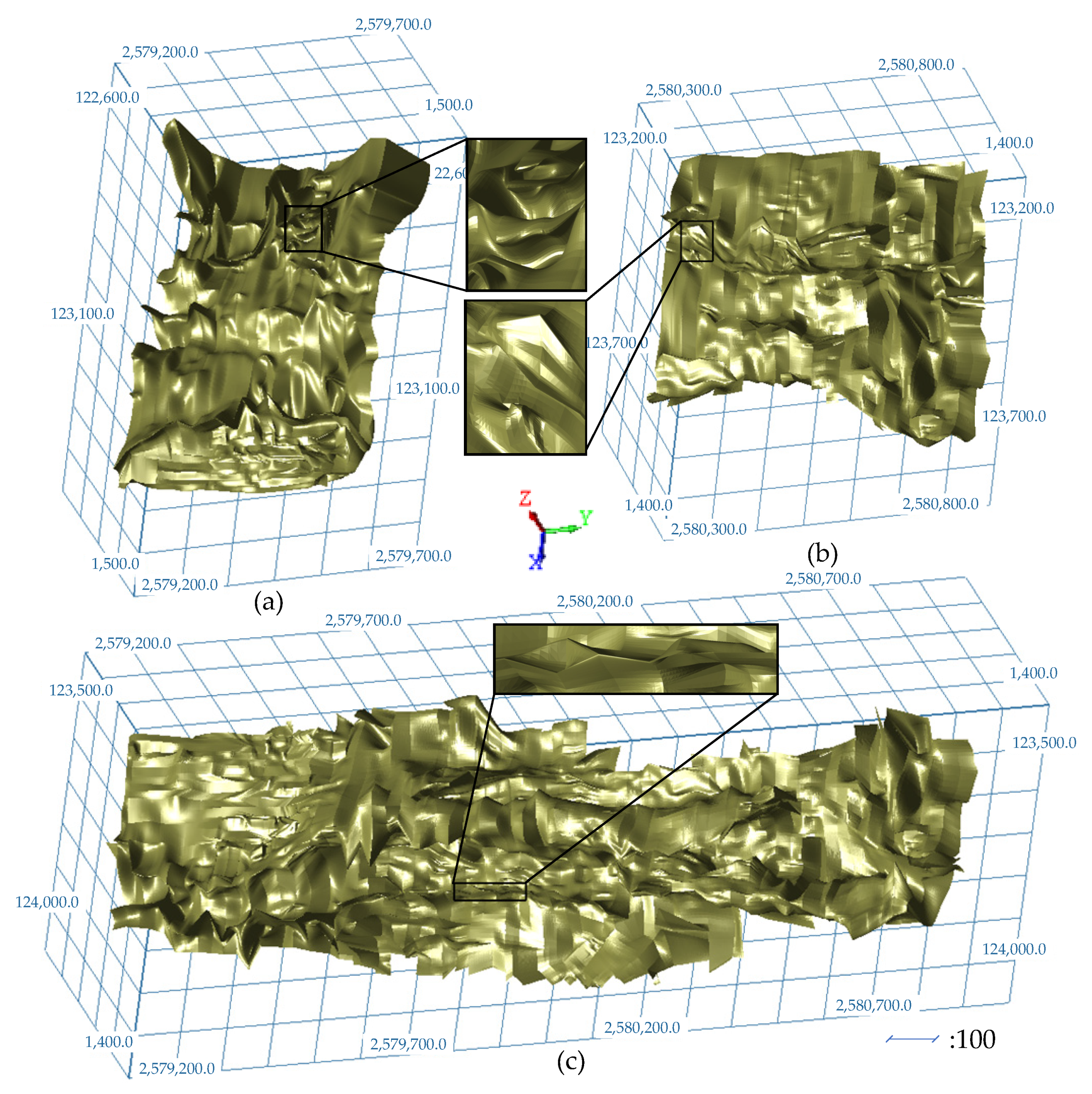
4.1. Examples
4.2. Discussion
5. Conclusions
Author Contributions
Funding
Acknowledgments
Conflicts of Interest
References
- Wang, B.; Shi, B.; Song, Z. A simple approach to 3D geological modelling and visualization. Bull. Eng. Geol. Environ. 2009, 68, 559–565. [Google Scholar]
- Jin, B.-X.; Fang, Y.-M.; Song, W.-W. 3D visualization model and key techniques for digital mine. Trans. Nonferrous Met. Soc. China 2011, 21, s748–s752. [Google Scholar] [CrossRef]
- Mallet, J.-L. Geomodeling; Oxford University Press: New York, NY, USA, 2002; p. 624. [Google Scholar]
- Jessell, M. Three-dimensional geological modelling of potential-field data. Comput. Geosci. 2001, 27, 455–465. [Google Scholar] [CrossRef]
- Feltrin, L.; Mclellan, J.G.; Oliver, N. Modelling the giant, Zn–Pb–Ag Century deposit, Queensland, Australia. Comput. Geosci. 2009, 35, 108–133. [Google Scholar] [CrossRef] [Green Version]
- Vollgger, S.A.; Cruden, A.R.; Ailleres, L.; Cowan, E.J. Regional dome evolution and its control on ore-grade distribution: Insights from 3D implicit modelling of the Navachab gold deposit, Namibia. Ore Geol. Rev. 2015, 69, 268–284. [Google Scholar] [CrossRef]
- Tungyshbayeva, Z.; Royer, J.J.; Zhautikov, T.M. 3D modeling and resources estimation of a gold deposit, Zhungarie province, Kazakhstan. In Proceedings of the 13th SGA Biennial Meeting on Mineral Resources in a Sustainable World, Nancy, France, 24–27 August 2015; pp. 1759–1761. [Google Scholar]
- Leapfrog. 2013. Available online: http://www.leapfrog3d.com (accessed on 1 February 2022).
- Royer, J.J.; Mejia, P.; Caumon, G.; Collon-Drouaillet, P. 3&4D geomodeling applied to mineral resources exploration—A new tool for targeting deposits. In Proceedings of the 12th SGA Biennial Meeting, Uppsala, Sweden, 12–15 August 2013. [Google Scholar]
- Coons, S.A. Surfaces for Computer-Aided Design of Space Forms; Technical Report MAC-TR-41; Massachusetts Institute of Technology: Cambridge, MA, USA, 1967. [Google Scholar]
- Zhong, D.-Y.; Wang, L.-G.; Bi, L.; Jia, M.-T. Implicit modeling of complex orebody with constraints of geological rules. Trans. Nonferrous Met. Soc. China 2019, 29, 2392–2399. [Google Scholar] [CrossRef]
- Hodgkinson, J.H.; Elmouttie, M. Cousins, siblings and twins: A review of the geological model’s place in the digital mine. Resources 2020, 9, 24. [Google Scholar] [CrossRef] [Green Version]
- Kong, T.; Zhang, Y.; Fu, X. The model of feature extraction for free-form surface based on topological transformation. Appl. Math Model 2018, 64, 386–397. [Google Scholar] [CrossRef]
- Yamany, S.; Farag, A. Surface signatures: An orientation independent free-form surface representation scheme for the purpose of objects registration and matching. IEEE Trans. Pattern Anal. Mach. Intell. 2002, 24, 1105–1120. [Google Scholar] [CrossRef]
- Saini, D.; Kumar, S. Free-form surface reconstruction from arbitrary perspective images. In Proceedings of the IEEE International Advance Computing Conference, ITM, Gurgaon, India, 21–22 February 2014; pp. 1054–1059. [Google Scholar] [CrossRef]
- Turk, G.; O’Brien, J.F. Modelling with implicit surfaces that interpolate. ACM Trans. Graph. 2002, 21, 855–873. [Google Scholar] [CrossRef]
- Yuan, Z.; Yu, Y.; Wang, W. Object-space multiphase implicit functions. ACM Trans. Graph. 2012, 31, 1–10. [Google Scholar] [CrossRef]
- Barthe, L.; Dodgson, N.A.; Sabin, M.A.; Wyvill, B.; Gaildrat, V. Two-dimensional Potential Fields for Advanced Implicit Modeling Operators. Comput. Graph. Forum 2003, 22, 23–33. [Google Scholar] [CrossRef] [Green Version]
- Farin, G. Smooth interpolation to scattered 3D data. In Surfaces in Computer Aided Geometric Design (Oberwolfach, 1982); Barnhill, R.E., Boehm, W., Eds.; North-Holland: Amsterdam, The Netherlands, 1983; pp. 43–63. [Google Scholar]
- Cheng, F.H.; Wang, X.F.; Barsky, B.A. Quadratic B-spline curve interpolation. Comput. Math. Appl. 2001, 41, 39–50. [Google Scholar] [CrossRef] [Green Version]
- Hu, S.-M.; Tai, C.-L.; Zhang, S.-H. An extension algorithm for B-splines by curve unclamping. Comput. Des. 2002, 34, 415–419. [Google Scholar] [CrossRef]
- Park, H. B-spline surface fitting based on adaptive knot placement using dominant columns. Comput. Des. 2011, 43, 258–264. [Google Scholar] [CrossRef]
- Krishnamurthy, A.; Khardekar, R.; McMains, S.; Haller, K.; Elber, G. Performing efficient NURBS modeling operations on the GPU. IEEE Trans. Vis. Comput. Graph. 2009, 15, 530–543. [Google Scholar] [CrossRef] [Green Version]
- Selimovic, I. Improved algorithms for the projection of points on NURBS curves and surfaces. Comput. Aided Geom. Des. 2006, 23, 439–445. [Google Scholar] [CrossRef]
- Wang, Q.; Hua, W.; Li, G.Q.; Bao, H.J. Generalized NURBS curves and surfaces. In Proceedings of the International Conference on Geometric Modeling and Processing, Beijing, China, 13–15 April 2004; pp. 365–368. [Google Scholar]
- Randrianarivony, M. On global continuity of Coons mappings in patching CAD surfaces. Comput. Des. 2009, 41, 782–791. [Google Scholar] [CrossRef]
- Farin, G.; Hansford, D. Discrete coons patches. Comput. Aided Geom. Des. 1999, 16, 691–700. [Google Scholar] [CrossRef]
- Hugentobler, M.; Schneider, B. Breaklines in Coons surfaces over triangles for the use in terrain modelling. Comput. Geosci. 2005, 31, 45–54. [Google Scholar] [CrossRef]
- Sapidis, N.S.; Besl, P.J. Direct construction of polynomial surfaces from dense range images through region growing. ACM Trans. Graph. 1995, 14, 171–200. [Google Scholar] [CrossRef]
- Hoppe, H.; Derose, T.; Duchamp, T.; McDonald, J.; Stuetzle, W. Surface reconstruction from unorganized points. ACM SIGGRAPH Comput. Graph. 1992, 26, 71–78. [Google Scholar] [CrossRef]
- Edelsbrunner, H.; Mücke, E. Three-dimensional alpha shapes. ACM Trans. Graph. 1994, 13, 75–82. [Google Scholar] [CrossRef]
- Fuchs, H.; Kedem, Z.M.; Uselton, S.P. Optimal surface reconstruction from planar contours. Commun. ACM 1977, 20, 693–702. [Google Scholar] [CrossRef]
- Keppel, E. Approximating complex surfaces by triangulation of contour lines. IBM J. Res. Dev. 1975, 19, 2–11. [Google Scholar] [CrossRef]
- Floater, M.S.; Reimers, M. Meshless parameterization and surface reconstruction. Comput. Aided Geom. Des. 2001, 18, 77–92. [Google Scholar] [CrossRef]
- Macedonio, G.; Pareschi, M. An algorithm for the triangulation of arbitrarily distributed points: Applications to volume estimate and terrain fitting. Comput. Geosci. 1991, 17, 859–874. [Google Scholar] [CrossRef]
- Meyers, D.; Skinner, S.; Sloan, K. Surfaces from contours. ACM Trans. Graph. (TOG) 1992, 11, 228–258. [Google Scholar] [CrossRef]
- Ekoule, A.B.; Peyrin, F.; Odet, C.L. A triangulation algorithm from arbitrary shaped multiple planar contours. ACM Trans. Graph. 1991, 10, 182–199. [Google Scholar] [CrossRef]
- Jones, M.W.; Min, C. A new approach to the construction of surfaces from contour data. Comput. Graph. Forum 2010, 13, 75–84. [Google Scholar] [CrossRef]
- Zhong, D.-Y.; Wang, L.-G.; Jia, M.-T.; Bi, L.; Zhang, J. Orebody modeling from non-parallel cross sections with geometry constraints. Minerals 2019, 9, 229. [Google Scholar] [CrossRef] [Green Version]
- Wu, Z.; Zhong, D.; Li, Z.; Wang, L.; Bi, L. Orebody modeling method based on the normal estimation of cross-contour polylines. Mathematics 2022, 10, 473. [Google Scholar] [CrossRef]
- Song, R.; Nan, J. The design and implementation of a 3D orebody wire-frame modeling prototype system. In Proceedings of the Second International Conference on Information and Computing Science, Manchester, UK, 21–22 May 2009; Volume 2, pp. 357–360. [Google Scholar] [CrossRef]
- Jessell, M.; Ailleres, L.; De Kemp, E.; Lindsay, M.; Wellmann, F.; Hillier, M.; Laurent, G.; Carmichael, T.; Martin, R. Next generation three-dimensional geologic modeling and inversion. In Building Exploration Capability for the 21st Century; Kelley, K.D., Golden, H.C., Eds.; Soc Economic Geologists, Inc.: Littleton, CO, USA, 2014; pp. 261–272. [Google Scholar]
- Knight, R.H. Orebody solid modelling accuracy—A comparison of explicit and implicit modelling techniques using a practical example from the Hope Bay District, Nunavut, Canada. In Proceedings of the 6th International Mining Geology Conference, Darwin, Australia, 21–23 August 2006; pp. 175–183. [Google Scholar]
- Lipuš, B.; Guid, N. A new implicit blending technique for volumetric modelling. Vis. Comput. 2005, 21, 83–91. [Google Scholar] [CrossRef]


| Plane Bit | α | β | γ | δ | ε | |
|---|---|---|---|---|---|---|
| Segments | ||||||
| a | 1 | 0 | 2 | 1 | 1 | |
| b | 1 | 1 | 2 | 1 | 0 | |
| c | 1 | 1 | 0 | 1 | 1 | |
| d | 1 | 1 | 2 | 0 | 1 | |
| Plane bit | α | β | γ | δ | ε | |
|---|---|---|---|---|---|---|
| Segments | ||||||
| a1 | 1 | 1 | 2 | 1 | 1 | |
| a2 | 1 | 2 | 2 | 1 | 1 | |
| b1 | 1 | 1 | 2 | 1 | 1 | |
| b2 | 1 | 1 | 2 | 1 | 2 | |
| c1 | 1 | 1 | 1 | 1 | 1 | |
| c2 | 1 | 1 | 2 | 1 | 1 | |
| d1 | 1 | 1 | 2 | 1 | 1 | |
| d2 | 1 | 1 | 2 | 2 | 1 | |
Publisher’s Note: MDPI stays neutral with regard to jurisdictional claims in published maps and institutional affiliations. |
© 2022 by the authors. Licensee MDPI, Basel, Switzerland. This article is an open access article distributed under the terms and conditions of the Creative Commons Attribution (CC BY) license (https://creativecommons.org/licenses/by/4.0/).
Share and Cite
Wu, Z.; Bi, L.; Zhong, D.; Zhang, J.; Tang, Q.; Jia, M. Orebody Modeling Method Based on the Coons Surface Interpolation. Minerals 2022, 12, 997. https://doi.org/10.3390/min12080997
Wu Z, Bi L, Zhong D, Zhang J, Tang Q, Jia M. Orebody Modeling Method Based on the Coons Surface Interpolation. Minerals. 2022; 12(8):997. https://doi.org/10.3390/min12080997
Chicago/Turabian StyleWu, Zhaohao, Lin Bi, Deyun Zhong, Ju Zhang, Qiwang Tang, and Mingtao Jia. 2022. "Orebody Modeling Method Based on the Coons Surface Interpolation" Minerals 12, no. 8: 997. https://doi.org/10.3390/min12080997