Article

NHF as an Edge Detector of Potential Field Data and Its Application in the Yili Basin

1
School of Geophysics and Information Technology, China University of Geosciences, Beijing 100083, China
2
Department of Earth and Space Sciences, Southern University of Science and Technology, Shenzhen 518055, China
*
Author to whom correspondence should be addressed.
Minerals 2022, 12(2), 149; https://doi.org/10.3390/min12020149
Submission received: 20 December 2021 / Revised: 24 January 2022 / Accepted: 25 January 2022 / Published: 27 January 2022

Abstract

:
Edge enhancement is a frequently used transformation of potential field data. Its goal is to sharpen the position of the subsurface structures. Here we propose a new method to enhance the edges of the sources causing the potential anomalies called normalized Harris filter (NHF), which is based on the Harris filter and amplitude balance. Three synthetic data sets are used to evaluate the performance of the proposed approach. The presented approach provides a better estimation of the sources’ edges when compared to the other methods. The proposed method is robust to noisy data and can avoid the generation of artificial edges, thereby reducing the ambiguity of interpretation. The testing on real data set from the Yili basin in Northwestern China demonstrates that the new approach highlights several anomalies not shown in the geological map or other methods. The proposed approach also shows the advantages of gradually enhancing the edges of the deep-seated structure. The results demonstrate that the proposed approach may be a better detector in qualitatively determining the edges of sources causing potential field data.

1. Introduction

Potential field data contains all the signals from geological bodies with different locations and geometries and has a volume effect. Many data processing techniques have been developed to facilitate the interpretation. In recent years, edge enhancement has received increasing attention, benefiting from its simplicity and effectiveness. The main purpose of edge enhancement is to delineate the edges and positions of the subsurface structures. The most popular edge detectors are total horizontal derivative [1] (THD, Equation (1)), tilt angle [2] (TA, Equation (2)), THD of tilt angle [3] (THDT, Equation (3)), theta map [4] (theta, Equation (4)), the tilt angle of the THD [5] (TAHG, Equation (5)), the tilt angle of the analytic signal amplitude [6] (TASA, Equation (6)). The approaches mentioned above have been evaluated in many works [7,8,9,10,11]. In addition to THD, other approaches involve calculating the vertical derivative or second-order derivative of the potential field data, which causes the amplified noise in the data. Therefore, it is necessary to perform denoising before or after the derivative process.
THD = ( f x ) 2 + ( f y ) 2
TA = arctan ( f / z THD )
THDT = ( TA x ) 2 + ( TA y ) 2
c o s ( θ ) = THD ASA
TAHG = arctan ( THD / z ( THD d x ) 2 + ( THD d y ) 2 )
TASA = arctan ( ASA / z ( ASA x ) 2 + ( ASA y ) 2 )
with:
ASA = ( f x ) 2 + ( f y ) 2 + ( f z ) 2
where f denotes the potential field data.
Image processing techniques have been widely used in geophysics. For example, Ref. [12] employed sun shading to extract the features from potential field data. Ref. [13] used the Sobel filter to detect the fault and salt boundary. Ref. [14] used the 2D Gabor filter on the magnetic data to interpret the subsurface lineaments. Ref. [15] used the Canny filter [16] to perform the edge-guided full-waveform inversion. Ref. [17] employed phase congruency to detect lineaments embedded in magnetic data. The Harris filter [18,19] provides strong invariance to rotation, scaling, and noise. It has been widely used in many scientific areas based on image processing techniques, such as camera calibration [20], image stitching [21], and unstructured finite-element meshing [22].
In this work, we employ the Harris filter to detect the edges of the subsurface structures from potential field data. Amplitude balance is applied to equalize the response from the sources at different depths. Depth scales can range from kilometers to meters, depending on the resolution of the data. Source edges are characterized by maxima of the normalized Harris filter (NHF) response. The NHF will be evaluated using three synthetic data sets. The capabilities of NHF to handle noisy data and complex sources are described. Finally, we apply the NHF to real gravity data from the Yili basin.

2. Normalized Harris Filter

2.1. The Harris Filter

Following [18], the change E in the potential field data f (with a size of m × n) produced by a small shift (u, v) is given by (details are provided in Appendix A)
E = A u 2 + 2 C u v + B v 2 = ( u , v ) M ( u , v ) T
where the local structure matrix M is defined by:
M = ( A C C B )
The horizontal derivatives A and B, and diagonal derivative C are defined as:
A = i = 1 n ( f x ) 2
B = i = 1 n ( f y ) 2
and:
C = i = 1 n ( f x f y )
where n corresponds to the number of neighbors in the four directions (along the row, column, and diagonals) of f within the small shift.
The response function R of the Harris filter is defined as:
R = D e t ( M ) + μ T r 2 ( M )
where Det represents the determinant of M and Det(M) = AB − C2; Tr represents the trace of M and Tr(M) = A + B; μ is a user-specified parameter, which defines the sharpness or smoothness of the response function R and μ ∈ [0, 1]. The Harris filter response of the f can be stored in a grid R in the same size as f:
R = ( R 1 , 1 R 1 , 2 R 1 , n R 2 , 1 R 2 , 1 R 2 , n R m , 1 R m , 2 R m , n )
A moving window of size 3 × 3 and Equation (13) are employed to compute the elements of the R. The edge/corner areas are determined by the amplitude of the elements in R. If Rij is a local maximum within its neighbors, Rij will be considered as a candidate of edge/corner.

2.2. Amplitude Balance

Although the local maxima of R can delineate edges of the source, their amplitudes vary greatly. We employ a multi-step normalization technique to balance the amplitude of the local maxima of R. Thus; all edges are featured by a fixed value of 1.
(i)
Pick out the local maxima of R
We adopt the method of [23] to pick out the local maxima of R. The method compares each Ri,j (except the marginal rows and columns, i ∈ [1, m] and j ∈ [1, n]) and its eight nearest neighbors in four directions (along rows, columns, and two diagonals). If Ri,j is greater than its neighbors in at least two directions, it is regarded as a candidate of local maximum [24].
(ii)
Threshold of the local maxima
Some local maxima can be named as invalid, while they produce artifacts (false edges) in the solutions. Therefore, threshold processing is necessary to suppress the local maxima related to noise. If a local maximum is less than the threshold
threshold = λ·max(R)
it will be disqualified from the candidate of the local maximum. In theory, λ is limited to between 0 and 1. For different data sets, the optimal value of λ may be different.
(iii)
Calculate the upper envelope surface of the R
We employ the local maxima above the threshold to interpolate the upper envelope surface, and the natural neighborhood method [25] is used. For the upper envelope surface boundary, we increase their values by 0.1 times the maximum of R. This will most likely guarantee that the upper envelope surface is always above R.
(iv)
Normalize R using upper envelope surface
The normalized Harris filter (NHF) response is the ratio of R to the upper envelope surface, and its maxima (with a fixed value of 1) represent the source edges.

3. Synthetic Data

This section applies the proposed approach to three synthetic data sets to evaluate its performance. All derivatives are calculated in the frequency domain. Three scenarios are considered as follows:

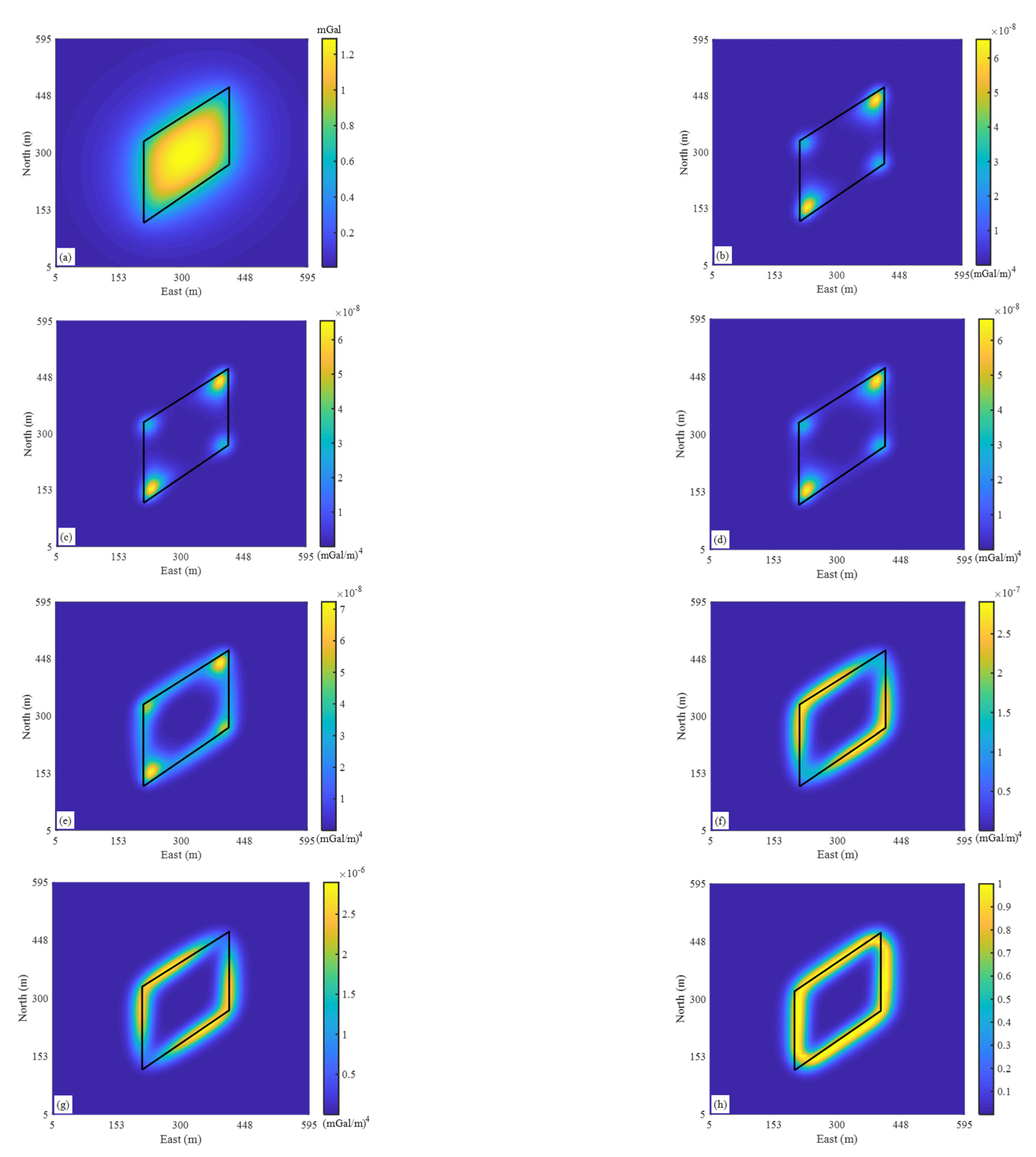
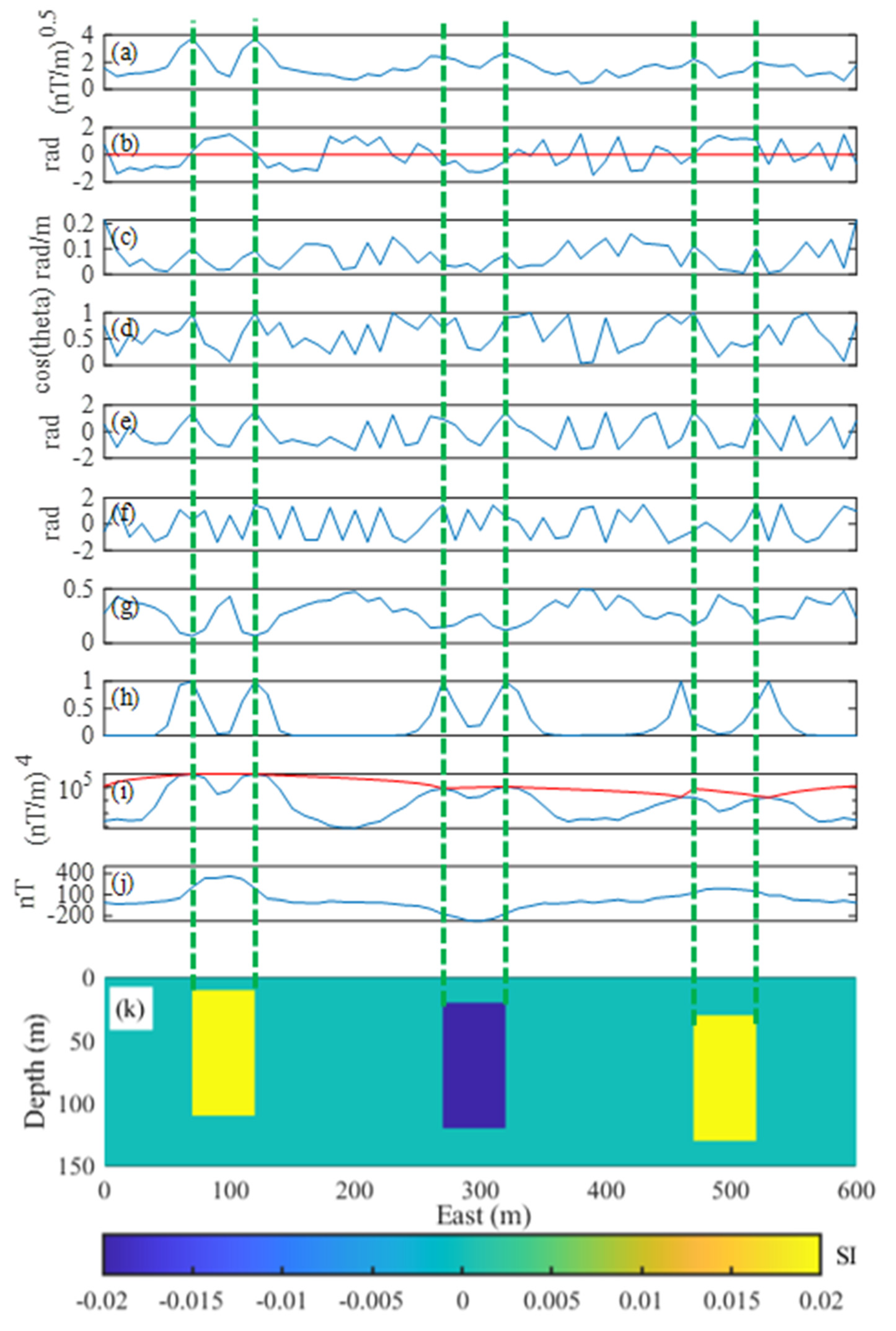
3.1. The Single Parallelepiped
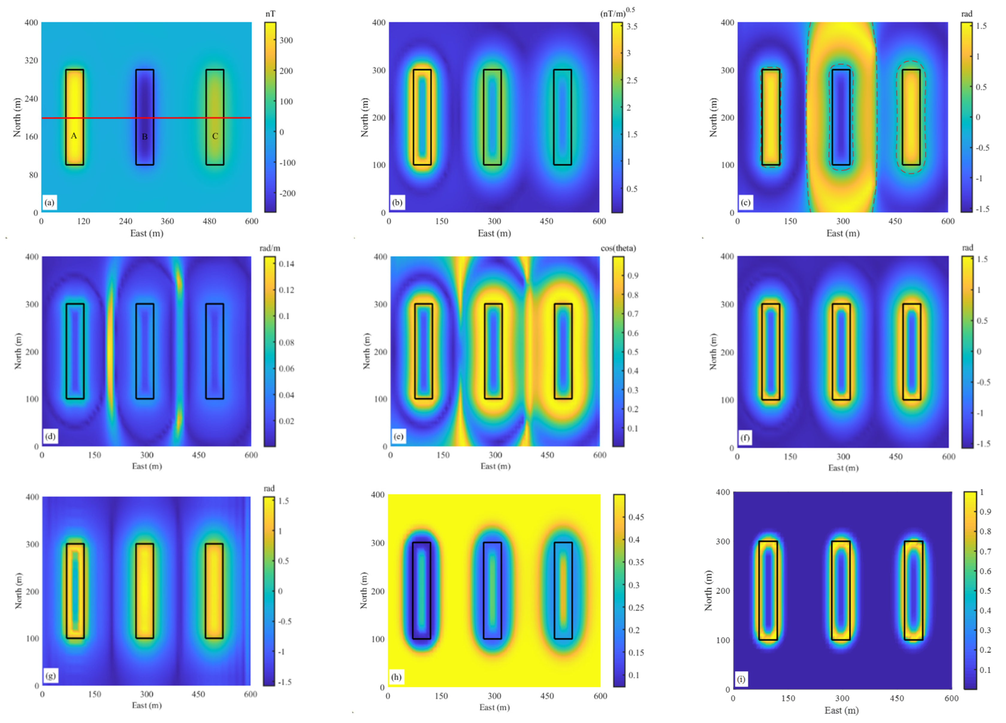
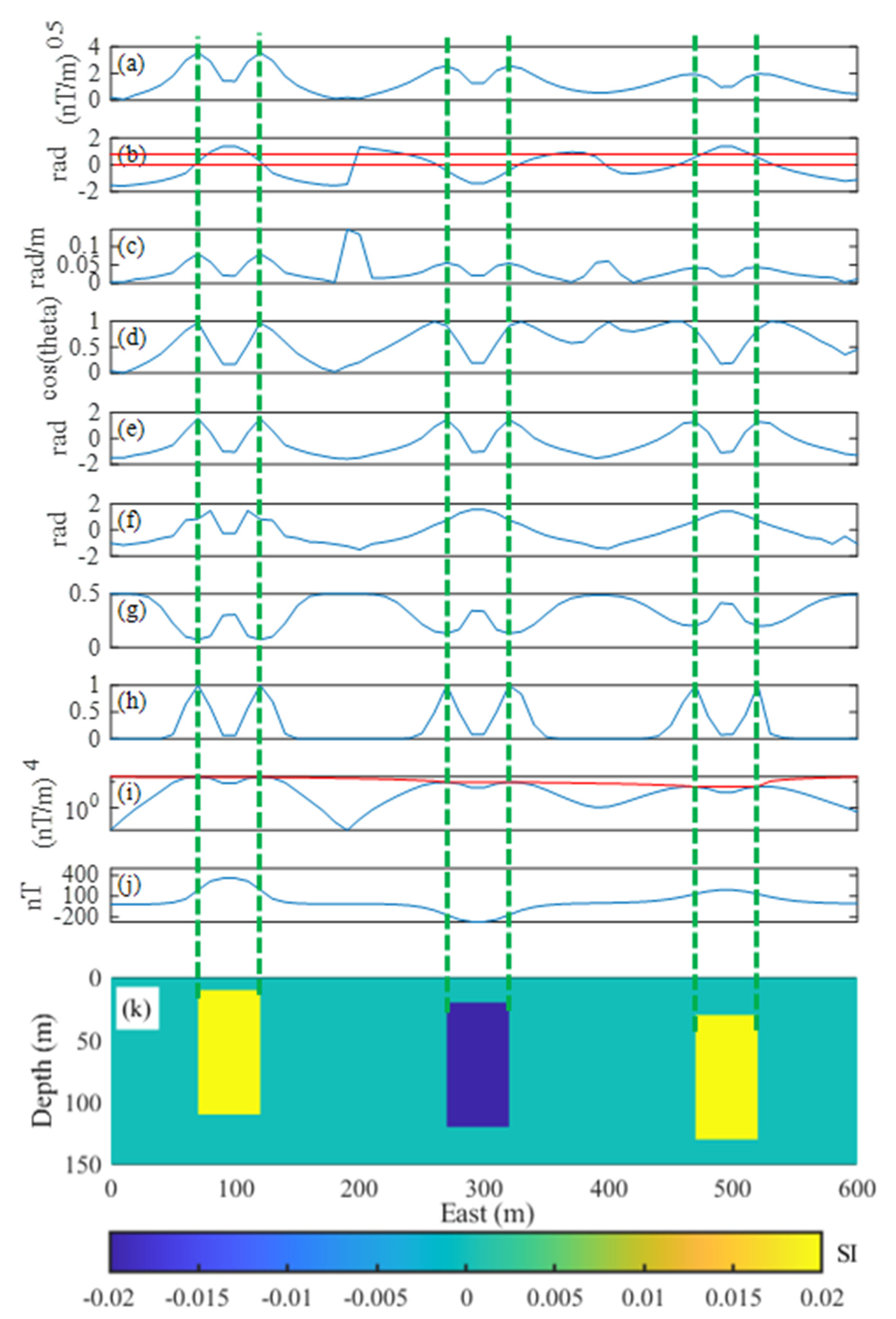
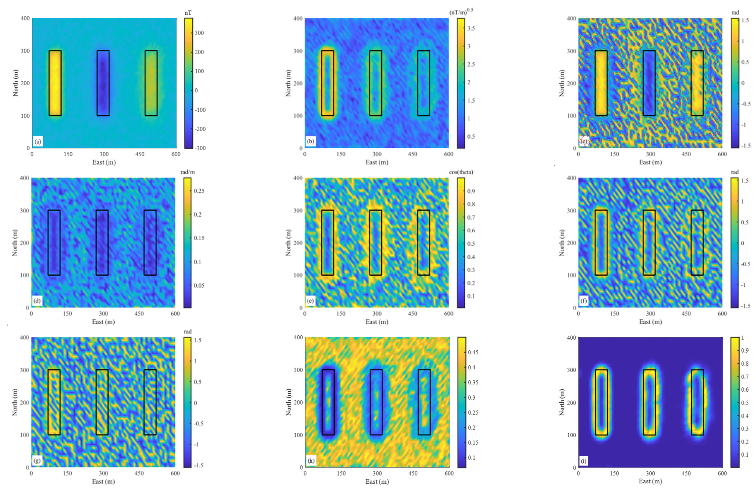
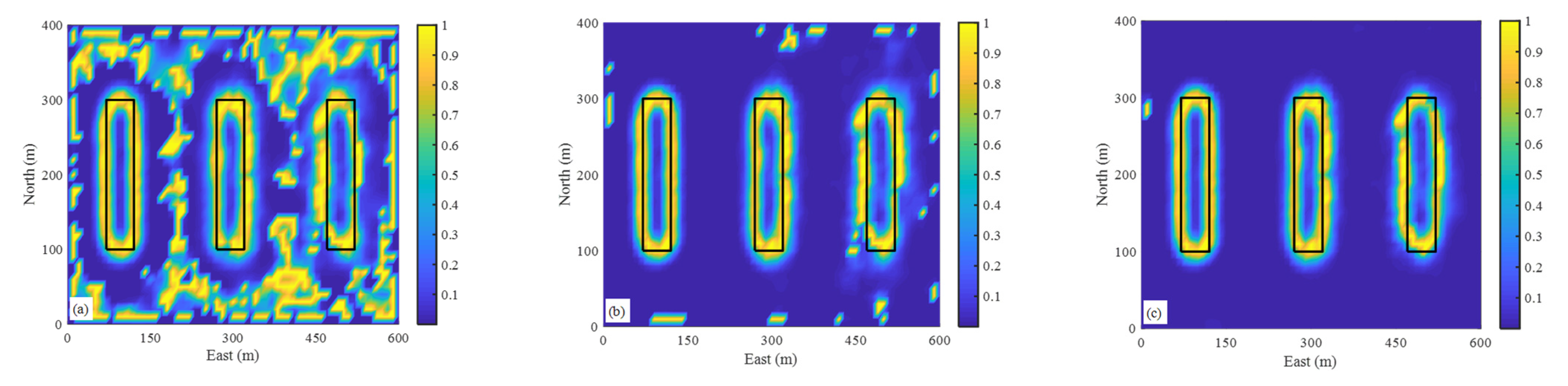
We have generated a single parallelepiped located at a depth of 20 m to assess the feasibility of the proposed approach. Figure 1a shows the noise-free gravity anomaly (with a grid interval of 10 m) produced by the parallelepiped with a density of 1.0 g/cm3, where the black lines indicate the actual edges.
Figure 1b–g show the Harris filter response of the data in Figure 1a with different empirical parameters μ. All corners and edges are characterized by local maxima. Furthermore, a small μ value allows the Harris filter to detect only the sharpest corners of the source (Figure 1b–d), and as the μ value increases, edges of the source are detected. When μ equals 0.1 and 1.0, the edges of the source can be clearly observed (Figure 1f,g). Figure 1h shows the NHF response. It demonstrates that the NHF response is amplitude balanced, and maxima characterize the edges. In general, when the application of interest is edge detection, high μ is preferred. Based on the above results and the knowledge from [18], we set the value of μ in the following examples to 1, unless otherwise noted.

3.2. Three Prisms

To further examine the proposed approach’s capability, we employ a model consisting of three prisms located at different depths [5]. The prisms have the same size (length = 200 m; width = 50 m; thickness = 100 m) with their tops located at depths 10 m (A), 20 m (B), and 30 m (C), and separated by distances of 200 m. The prisms are in the geomagnetic field: inducing field intensity B = 54,491 nT, direction (D, I) = (0°, 90°), and magnetic susceptibility of A, B, and C are 0.02 SI, −0.02 SI, and 0.02 SI, respectively. Figure 2a shows the magnetic anomalies of three prisms. We chose seven frequently used approaches to compare the results. They are THD [1], tilt angle [2], sun shading [12], THDT [3], theta map [4], TAHG [5], and tilt–ASA [6]. To reduce the long-tailed histogram of THD, we plot the square root of THD in this and the following sections.
We assess the proposed approach’s performance to detect edges from anomalies with different amplitudes and compare the results with other approaches. Figure 2b–h show THD, tilt angle, THDT, theta map, TAHG, tilt–ASA, and the sun shading response of the data in Figure 2a. Figure 3 presents profile data (the location is shown in Figure 2a with a red line) to provide insightful details. THD is presented by maxima at the edges of the sources, and the strength of the THD is gradually attenuated with depth. The tilt angle equalizes the response from the anomalies at different depths, and the zero values of the tilt angle can be used to trace the edges [26]. However, there are some erroneous edges between different prisms. THDT delineates the edges by maxima, but the amplitude of THDT decreases as the source’s depth increases. Also, some wrong edges pollute the map. Theta map produces the edges of sources by maxima; however, for deep sources, the maxima are shifted out from the actual edges, making the sources appear bigger than they are. Similar to THDT, erroneous edges appeared in the results of the theta map. The TAHG balances the response of sources from different depths and shows maxima at the edges of the sources, as expected for TAHG that uses second-order derivatives. Like the tilt-angle, the tilt-ASA displays the edges with zero values [6]. The sun shading presents the minima at the edges of the sources, and its strength gradually decreases with depth. In the implementation of NHF, we set λ to 10−3. It is found that the NHF response clearly and focused characterizes edges of sources at different depths.
Noise is an unavoidable factor in interpreting real field data. Figure 4 shows the robustness of different approaches to noisy data. Figure 4a shows the magnetic anomaly in Figure 2a by adding independent Gaussian noise. Noise is added to data with the following equation:
d i n = d i + n o r m r n d ( m u , s t d )
with:
s t d = ( d max d min ) p e r c e n t m u = 0
where d i n is the noisy datum; di is the noise-free datum; normrnd is the Matlab built-in function, which generates a random number from the normal distribution with mean parameter mu and standard deviation parameter std; dmin is the minimum value of noise-free data; dmax is the maximum value of noise-free data. The percent is set to 2% in the noisy data test.
Figure 4 displays the results of the noisy data test. Figure 5 shows a depth section of the synthetic model and responses of different edge detectors. In general, all results are affected by the noise, and as the source depth increases, this effect becomes more serious. Specifically, Figure 4b shows that THD is less sensitive to noise. The tilt angle map equalizes the anomaly amplitudes, and it is less sensitive to noise than THDT, theta map, TAHG, and tilt–ASA. The edges recognized by the THDT are very blurred. The theta map can only roughly identify the edges of the sources. TAHG and tilt–ASA are particularly sensitive to noise and can almost only reflect the edge of a shallow source. Sun shading is less sensitive to the noise, and the recognition effect deteriorates as the source depth increases. Figure 4i shows the NHF response (λ = 1.2 × 10⁻²), and its maxima outline the sources’ edges. It shows that the proposed approach is capable of handling noisy data.
To illustrate the choice of parameters, we change λ for noisy data tests. Figure 6 shows the NHF response of the data in Figure 4a with different parameters. A small λ value can cause erroneous edges related to noise, and a large λ value can suppress the noise effect. In this case, an λ of 1.2 × 10⁻² produces satisfactory results (Figure 4i). This is a benefit of the proposed approach because it can be adapted to handle noise data.

3.3. The Bishop Model

We use the Bishop model’s magnetic anomaly to illustrate the proposed approach’s performance in the case of complex sources. Various authors have used the Bishop model to test approaches of estimating source depths using magnetic data [27,28,29]. Figure 7a displays the magnetic anomalies for a basement susceptibility varying from 1.26 × 10⁻² to 1.0 × 10⁻¹ SI units and an ambient geomagnetic field with strength 50,000 nT, declination 0°, and inclination 90°.
The THD, tilt angle, THDT, theta map, TAHG, tilt–ASA, and sun shading are shown in Figure 7b–h, respectively. It can be seen that all approaches generate the main features of shallow sources. Among them, TAHG provides improved structural details yet contains very little information for deep structures (the southeast part of the figure). We can also find that tilt-ASA shows some striped artifacts in the east and south parts of the figure. Figure 7i–l show the NHF responses with different choices of λ. As λ decreases, we can enhance our understanding of the edges of subsurface structures. Specifically, the NHF response generated by the large λ corresponds to the edges of the main structures, and the small λ can extract the edges associated with the minor structures.

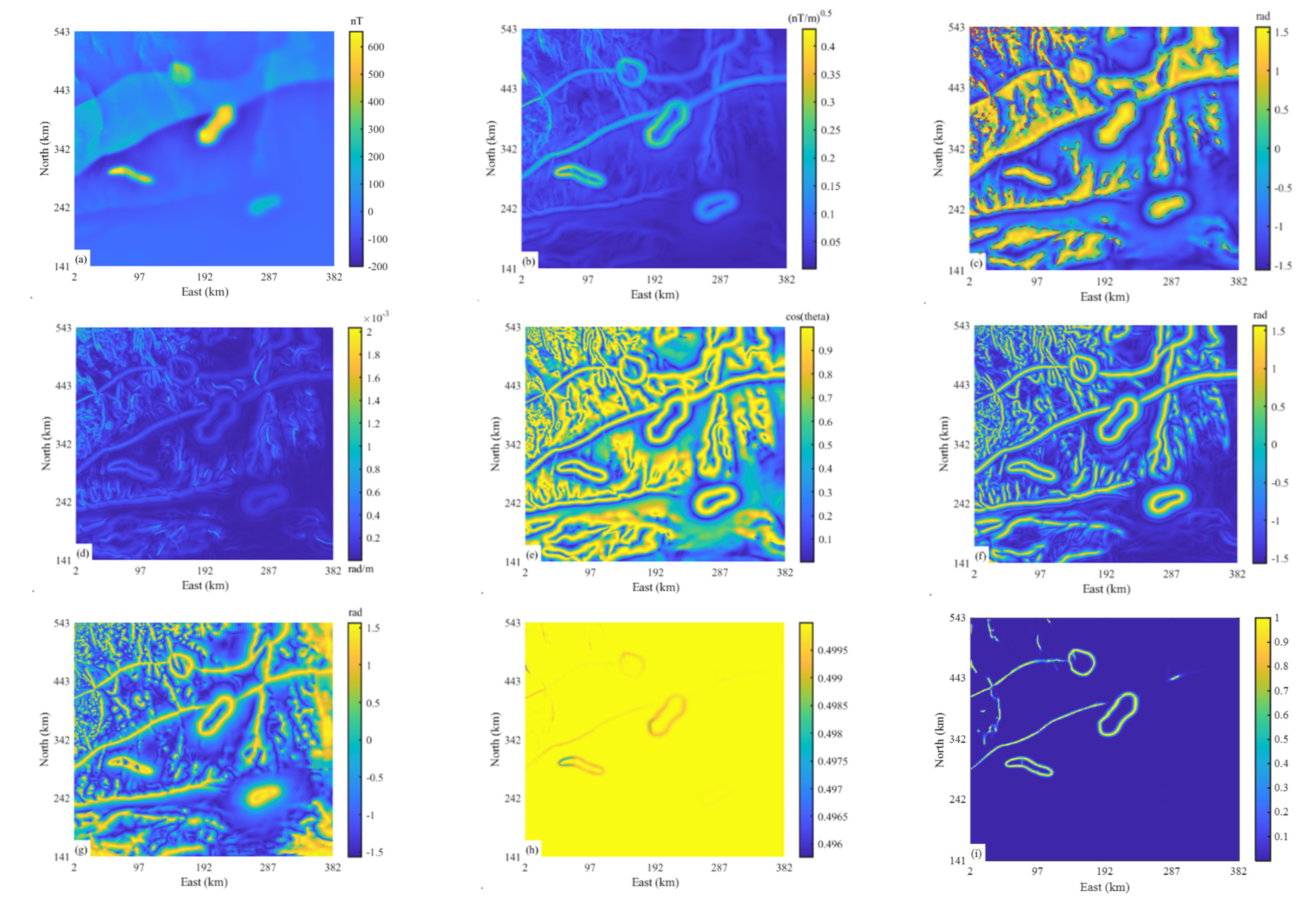
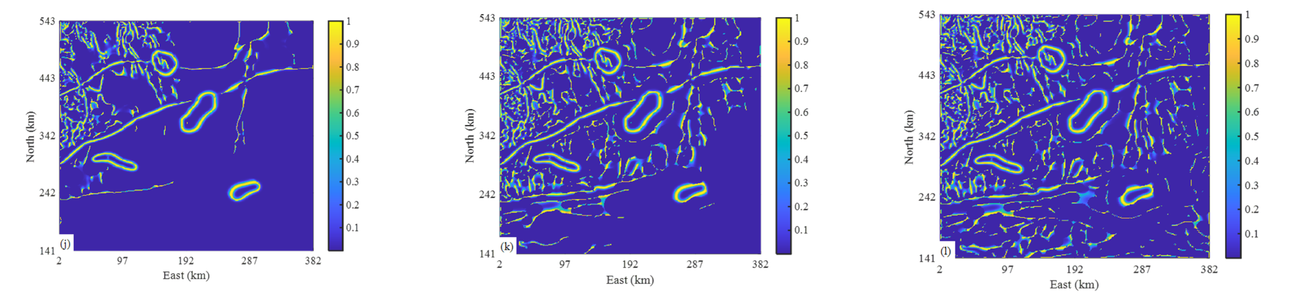
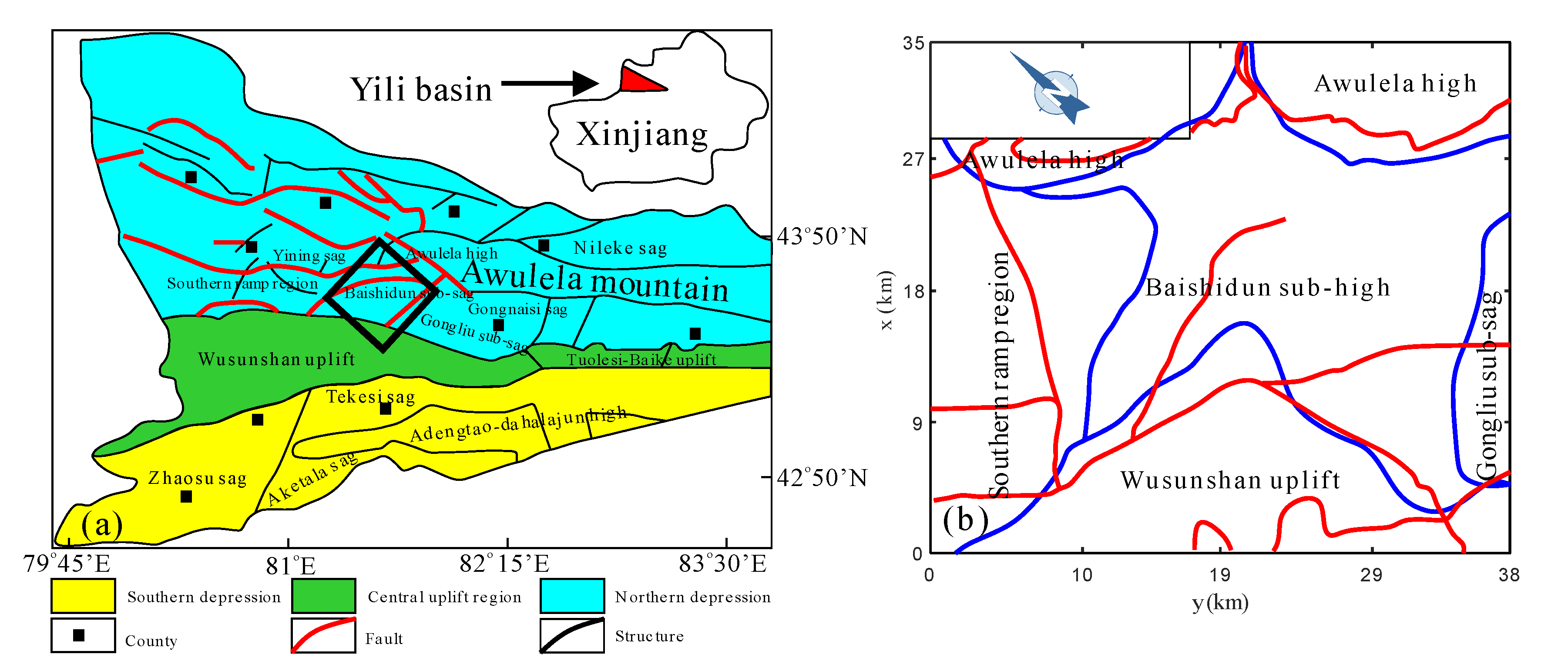
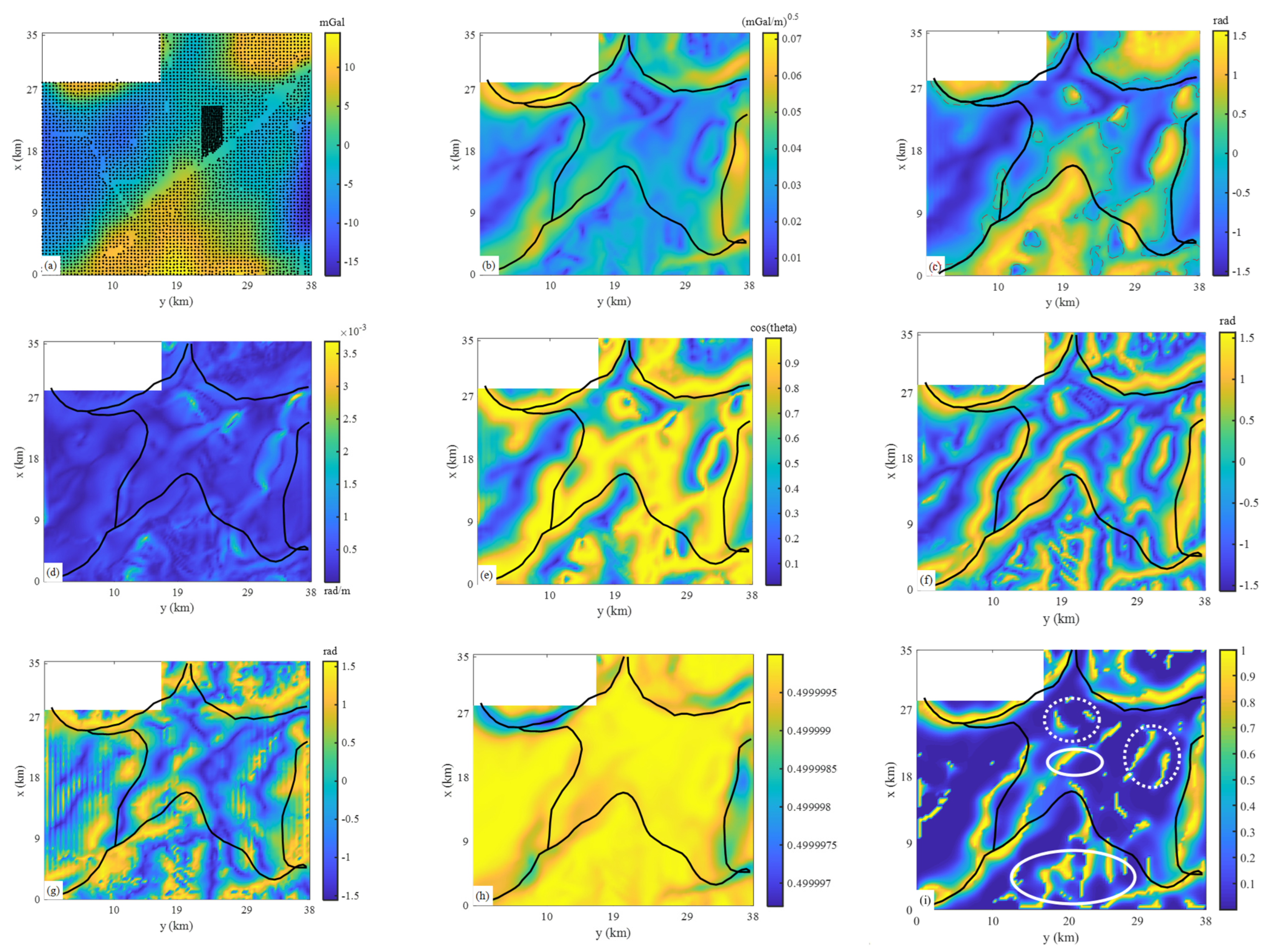
4. Field Gravity Data from Yili Basin

We will now discuss applying the proposed approach to gravity data collected from Xinjiang, northwestern China (Figure 8a). The study area is located in the middle portion of the Yili Basin, centered on the Baishidun sub-high, covering an area of about 1200 km2. Tectonic units in the study area include Awulela high, Baishidun sub-high, Gongliu sub-sag, Southern ramp region, and Wusunshan uplift. The geological structure map of the study area is given in Figure 8b. The red lines indicate the structures inferred from the historical geophysical data, while the blue lines present the structures deduced from newly collected gravity data [30]. There is no clear understanding of the structural edges of the study area.
The gravity data has been gridded in 500 m intervals. Figure 9a shows the Bouguer anomaly of the study area. Similar to the previous sections, we compare the proposed approach with other approaches, and the results are shown in Figure 9b–h. From Figure 9, we can see that these approaches enhance the main structures. However, it shows that the TAHG and tilt-ASA carry severe striped artifacts because they all use high-order derivatives, and the calculation of high-order derivatives is easily affected by the conflicting information contained in the actual data [32]. The proposed approach (with λ = 10−5) produces focused results (Figure 9i) and clarifies the structures.
When comparing the NHF response (Figure 9i) with known geological structures (Figure 8b), edges of the Awulela high, the Wusunshan uplift, the Gongliu sub-sag, and the Southern ramp region are consistent with the blue lines in Figure 8b. Some minor structures (white solid ellipses in Figure 9i) in the Wusunshan uplift and Baishidun sub-high are compatible with red lines in Figure 8b. These results suggest that edge enhancement can bridge the gap between different prior information. Structures in the Baishidun sub-high (white dashed ellipses in Figure 9i) are identified in the NHF response but not marked on the geological map (Figure 8b); this means that edge enhancement can help the interpreter enrich the knowledge of subsurface structures.

5. Conclusions

In this study, the applicability of NHF to potential field data is shown to enhance the edges of the subsurface structures. The edges are identified by fixed value 1 in the NHF response. The NHF involves an adjustable parameter λ. The choice of λ depends on the quality of the potential field data. When data quality is poor, a higher λ is required to obtain an interpretable result (Figure 4 and Figure 6). When the data quality is acceptable, λ can be adjusted to enhance the understanding of edges from different structures (Figure 7). In this case, NHF can be regarded as a gain-controlled edge detector.
The proposed approach has been tested using three synthetic data sets. For the single parallelepiped example, we have demonstrated that setting the empirical parameter μ to 1 can improve the sensitivity of NHF to the source edges. For three prisms example, the effectiveness of the NHF for sources at different depths is illustrated. Furthermore, the results show that a larger λ can aid the NHF against noise. For magnetic data caused by the Bishop model, we present the capability of NHF as a gain control edge detector. In the case of complex sources, NHF can enhance our understanding of the edges of different sources. Finally, the proposed approach was applied to the gravity data collected in the Yili Basin. The results are compared with previous studies, and it can be seen that edge enhancement is a valuable tool for characterizing structural edges.

Author Contributions

Conceptualization, T.C.; methodology, T.C.; writing—original draft preparation, T.C.; writing—review and editing, G.Z.; visualization, T.C.; supervision, G.Z.; project administration, G.Z.; funding acquisition, G.Z. All authors have read and agreed to the published version of the manuscript.

Funding

This work was supported in part by the Terrestrial and Oceanic Geological Map Updating and Sharing Program of China (grant number DD20190370), in part by Stable-Support Scientific Project of China Research Institute of Radiowave Propagation (grant number A132007W06), and in part by the National Natural Science Foundation of China (grant number 41630320).

Institutional Review Board Statement

Not applicable.

Informed Consent Statement

Not applicable.

Data Availability Statement

The data underlying this article will be shared on reasonable request to the corresponding author. The code associated with this paper can be found at https://github.com/GeoGoku/EdgeEnhancement (accessed on 3 June 2021). The users can redistribute it and/or modify it under the terms of the GNU General Public License.

Acknowledgments

We are grateful to Tianlong Yan and Bin Hu for their discussions. We thank Gordon R. J. Cooper and Duncan R. Cowan for providing the gradient calculation scripts (publicly available at https://software.seg.org/2008/0001/, accessed on 19 March 2008).

Conflicts of Interest

The authors declare no conflict of interest.

Appendix A

Derivation of Equation (8).
The change E in the potential field data caused by a small shift ( u , v ) is defined as:
E ( u , v ) = [ f ( x + u , y + v ) f ( x , y ) ] 2
where f is the potential field data, with the Taylor series expansion, we have:
f ( x + u , y + v ) = f ( x , y ) + f x u + f x v + O ( u 2 , v 2 )
where f x and f y are partial derivatives of the f in x and y directions. Bringing Equation (A2) into Equation (A1):
E ( u , v ) = [ f x u + f x v + O ( u 2 , v 2 ) ] 2
Ignoring the high-order terms, the Equation (A3) becomes:
E ( u , v ) [ f x u + f y v ] 2 = ( ( f x ) 2 u 2 + 2 f x f y u v + ( f y ) 2 v 2 ) = [ u v ] [ ( f x ) 2 f x f y f x f y ( f y ) 2 ] [ u v ] = [ u v ] ( [ ( f x ) 2 f x f y f x f y ( f y ) 2 ] ) [ u v ] = [ u v ] M [ u v ]
with:
M = ( ( f x ) 2 f x f y f x f y ( f y ) 2 )

References

  1. Cordell, L.; Grauch, V. Mapping basement magnetization zones from aeromagnetic data in the San Juan Basin, New Mexico. In The Utility of Regional Gravity and Magnetic Anomaly Maps; Society of Exploration Geophysicists: Tusla, OK, USA, 1985; pp. 181–197. [Google Scholar]
  2. Miller, H.G.; Singh, V. Potential field tilt—A new concept for location of potential field sources. J. Appl. Geophys. 1994, 32, 213–217. [Google Scholar] [CrossRef]
  3. Verduzco, B.; Fairhead, J.D.; Green, C.M.; MacKenzie, C. New insights into magnetic derivatives for structural mapping. Lead. Edge 2004, 23, 116–119. [Google Scholar] [CrossRef]
  4. Wijns, C.; Perez, C.; Kowalczyk, P. Theta map: Edge detection in magnetic data. Geophysics 2005, 70, L39–L43. [Google Scholar] [CrossRef]
  5. Ferreira, F.J.; de Souza, J.; de B. e S. Bongiolo, A.; de Castro, L.G. Enhancement of the total horizontal gradient of magnetic anomalies using the tilt angle. Geophysics 2013, 78, J33–J41. [Google Scholar] [CrossRef]
  6. Cooper, G.R. Reducing the dependence of the analytic signal amplitude of aeromagnetic data on the source vector direction. Geophysics 2014, 79, J55–J60. [Google Scholar] [CrossRef]
  7. Fairhead, J.; Williams, S. Evaluating normalized magnetic derivatives for structural mapping. In SEG Technical Program Expanded Abstracts; Society of Exploration Geophysicists: Tusla, OK, USA, 2006; pp. 845–849. [Google Scholar]
  8. Li, X. On “Theta map: Edge detection in magnetic data” (C. Wijns, C. Perez, and P. Kowalczyk, 2005, Geophysics 71, L39–L43). Geophysics 2006, 71, X11. [Google Scholar] [CrossRef]
  9. Li, X. Understanding 3D analytic signal amplitude. Geophysics 2006, 71, L13–L16. [Google Scholar] [CrossRef]
  10. Li, X.; Pilkington, M. Attributes of the magnetic field, analytic signal, and monogenic signal for gravity and magnetic interpretation. Geophysics 2016, 81, J79–J86. [Google Scholar] [CrossRef]
  11. Pilkington, M.; Tschirhart, V. Practical considerations in the use of edge detectors for geologic mapping using magnetic data. Geophysics 2017, 82, J1–J8. [Google Scholar] [CrossRef]
  12. Cooper, G. Feature detection using sun shading. Comput. Geosci. 2003, 29, 941–948. [Google Scholar] [CrossRef]
  13. Aqrawi, A.A.; Boe, T.H. Improved fault segmentation using a dip guided and modified 3D Sobel filter. In SEG Technical Program Expanded Abstracts; Society of Exploration Geophysicists: Tusla, OK, USA, 2011; pp. 999–1003. [Google Scholar]
  14. Sertcelik, I.; Kafadar, O.; Kurtulus, C. Use of the two dimensional gabor filter to interpret magnetic data over the Marmara Sea, Turkey. Pure Appl. Geophys. 2013, 170, 887–894. [Google Scholar] [CrossRef]
  15. Xiang, S.; Zhang, H. Efficient edge–guided full–waveform inversion by Canny edge detection and bilateral filtering algorithms. Geophys. Suppl. Mon. Not. R. Astron. Soc. 2016, 207, 1049–1061. [Google Scholar] [CrossRef]
  16. Canny, J. A Computational Approach to Edge Detection. IEEE Trans. Pattern Anal. Mach. Intell. 1986, 8, 679–698. [Google Scholar] [CrossRef] [PubMed]
  17. Yalamanchili, S.R.; Hassan, H. Lineament Detection over Shale Gas Play of Horn River Basin Using Monogenic Phase Congruency of Magnetic Data. In Proceedings of the 78th EAGE Conference and Exhibition 2016, Vienna, Austria, 30 May–2 June 2016; pp. 1–5. [Google Scholar]
  18. Harris, C.G.; Stephens, M. A combined corner and edge detector. In Proceedings of the Alvey Vision Conference 1988, Manchester, UK, 31 August–2 September 1988; pp. 147–152. [Google Scholar]
  19. Schmid, C.; Mohr, R.; Bauckhage, C. Evaluation of interest point detectors. Int. J. Comput. Vis. 2000, 37, 151–172. [Google Scholar] [CrossRef] [Green Version]
  20. Cheng, O.; Guangzhi, W.; Quan, Z.; Wei, K.; Hui, D. Evaluating harris method in camera calibration. In Proceedings of the 2005 IEEE Engineering in Medicine and Biology 27th Annual Conference, Shanghai, China, 17–18 January 2005; pp. 6383–6386. [Google Scholar]
  21. Yao, G.; Cui, J.; Deng, K.; Zhang, L. Robust Harris corner matching based on the quasi–homography transform and self–adaptive window for wide–baseline stereo images. IEEE Trans. Geosci. Remote Sens. 2017, 56, 559–574. [Google Scholar] [CrossRef]
  22. Chou, T.-K.; Chouteau, M.; Dubé, J.-S. Intelligent meshing technique for 2D resistivity inverse problems. Geophysics 2016, 81, IM45–IM56. [Google Scholar] [CrossRef]
  23. Blakely, R.J.; Simpson, R.W. Approximating edges of source bodies from magnetic or gravity anomalies. Geophysics 1986, 51, 1494–1498. [Google Scholar] [CrossRef]
  24. Pawlowski, R.S. On: “Approximating edges of source bodies from magnetic or gravity anomalies” by RJ Blakely and RW Simpson (Geophysics 51, 1494–1498, July 1986). Geophysics 1989, 54, 1214. [Google Scholar] [CrossRef]
  25. Sibson, R. A brief description of natural neighbour interpolation. In Interpreting Multivariate Data; John, Wiley & Sons: Hoboken, NJ, USA, 1981. [Google Scholar]
  26. Oruç, B. Edge detection and depth estimation using a tilt angle map from gravity gradient data of the Kozaklı–Central Anatolia Region, Turkey. Pure Appl. Geophys. 2011, 168, 1769–1780. [Google Scholar] [CrossRef]
  27. Williams, S.E.; Fairhead, J.D.; Flanagan, G. Comparison of grid Euler deconvolution with and without 2D constraints using a realistic 3D magnetic basement model. Geophysics 2005, 70, L13–L21. [Google Scholar] [CrossRef]
  28. Salem, A.; Williams, S.; Fairhead, D.; Smith, R.; Ravat, D. Interpretation of magnetic data using tilt–angle derivatives. Geophysics 2008, 73, L1–L10. [Google Scholar] [CrossRef]
  29. Zhou, W.; Nan, Z.; Li, J. Self–constrained Euler deconvolution using potential field data of different altitudes. Pure Appl. Geophys. 2016, 173, 2073–2085. [Google Scholar] [CrossRef]
  30. Suo, K. Study on the Tectonic Characteristics of Central Yili Basin Based on Comprehensive Interpretation of Gravity and Magnetic Data. Ph.D. Thesis, China University of Geosciences, Beijing, China, 2016. (In Chinese). [Google Scholar]
  31. Xiong, L. Comprehensive Analysis of Yili Petroliferous Basin. Ph.D. Thesis, Northwest University, Xi’an, China, 2003. (In Chinese). [Google Scholar]
  32. Chen, T.; Yang, D. Joint inversion of time-domain and frequency-domain electromagnetic data contaminated by coherent noises using an agree-to-disagree strategy. In SEG Technical Program Expanded Abstracts; Society of Exploration Geophysicists: Tusla, OK, USA, 2020; pp. 565–569. [Google Scholar]
Figure 1. (a) Gravity anomaly of a single parallelepiped with a depth of 20 m and a density of 1.0 g/cm3. Harris filter response of the synthetic gravity anomaly in Figure 1a with μ value of (b) 1.0 × 10⁻⁵, (c) 1.0 × 10⁻⁴, (d) 1.0 × 10⁻³, (e) 1.0 × 10⁻², (f) 0.1 and (g) 1.0. (h) NHF response with λ = 0. The black lines outline the true edges.
Minerals 12 00149 g001
Figure 2. (a) Magnetic anomalies of three prisms with depths of 10 m (A), 20 m (B), and 30 m (C). TMI: inducing field intensity B = 54491 nT, direction (D, I) = (0°, 90°), and magnetic susceptibility 0.02 SI (A), −0.02 SI (B), and 0.02 SI (C). (b) The square root of THD of the data in (a). (c) Tilt angle of the data in (a). The dotted lines present zero contours. (d) THDT of the data in (a). (e) Theta map of the data in (a). (f) TAHG of the data in (a). (g) Tilt–ASA of the data in (a). (h) Sun shading using an elevation angle of 90°. (i) NHF response of the data in (a) (with λ = 10−3). The black rectangles outline the true edges.
Minerals 12 00149 g002
Figure 3. (a) The square root of THD. (b) Tilt angle, the red line shows the position where the tilt angle is zero. (c) THDT. (d) Theta map. (e) TAHG. (f) Tilt–ASA. (g) Sun shading using an elevation angle of 90°. (h) NHF response (with λ = 10−3). (i) HF response and its upper envelope (red line). (j) Profile data (the location is shown by a red line in Figure 2a). (k) A depth section of three prisms. Green dashed lines indicate the actual edges of the susceptibility bodies.
Minerals 12 00149 g003
Figure 4. (a) Magnetic anomaly in Figure 2a by adding 2% Gaussian noise. (b) The square root of THD of the data in (a). (c) Tilt angle of the data in (a). The dotted lines present zero contours. (d) THDT of the data in (a). (e) Theta map of the data in (a). (f) TAHG of the data in (a). (g) Tilt–ASA of the data in (a). (h) Sun shading using an elevation angle of 90°. (i) NHF response with λ = 1.2 × 10⁻². The black rectangles outline the true edges.
Minerals 12 00149 g004
Figure 5. (a) The square root of THD. (b) Tilt angle. The red line shows the position where the tilt angle is zero. (c) THDT. (d) Theta map. (e) TAHG. (f) Tilt–ASA. (g) Sun shading using an elevation angle of 90°. (h) NHF response (with λ = 1.2 × 10⁻²). (i) HF response and its upper envelope (red line). (j) Profile of noisy data (the location is shown by a red line in Figure 3a). (k) A depth section of three prisms. Green dashed lines indicate the actual edges of the susceptibility bodies.
Minerals 12 00149 g005
Figure 6. NHF response of the data in Figure 5a with (a) λ = 1.0 × 10⁻⁴, (b) λ = 1.0 × 10⁻³, (c) λ = 1.0 × 10⁻². The black boxes outline the true edges.
Minerals 12 00149 g006
Figure 7. (a) The magnetic anomaly of the Bishop model. (b) The square root of THD of the data in (a). (c) Tilt angle of the data in (a). The dotted line presents the zero contour. (d) THDT of the data in (a). (e) Theta map of the data in (a). (f) TAHG of the data in (a). (g) Tilt–ASA of the data in (a). (h) Sunshading using an elevation angle of 90°. (i) NHF response of the data in (a) (with λ = 1.0 × 10⁻³). (j) NHF response of the data in (a) (with λ = 1.0 × 10⁻⁶). (k) NHF response of the data in (a) (with λ = 1.0 × 10⁻⁹). (l) NHF response of the data in (a) (with λ = 0).
Minerals 12 00149 g007aMinerals 12 00149 g007b
Figure 8. (a) Tectonic units in Yili basin (after [31]). The black rectangle indicates the study area. (b) Simplified geological structure of the study area (after [30]), the red lines and blue lines indicate two possible structural divisions.
Minerals 12 00149 g008
Figure 9. (a) Bouguer anomaly of the study area. The black dots denote the location of the gravity stations. (b) The square root of THD of the data in (a). (c) Tilt angle of the data in (a). The dotted line presents the zero contour. (d) THDT of the data in (a). (e) Theta map of the data in (a). (f) TAHG of the data in (a). (g) Tilt–ASA of the data in (a). (h) Sun shading using an elevation angle of 90°. (i) NHF response of the data in (a) (with λ = 10−5). The black lines outline the known structures (blue lines in Figure 8b).
Minerals 12 00149 g009
Publisher’s Note: MDPI stays neutral with regard to jurisdictional claims in published maps and institutional affiliations.

