Improved Integral Equation Method for Rapid 3-D Forward Modeling of Magnetotelluric

Abstract

Computational cost tremendously restricts the wide application of conventional integral equation (IE) method in large-scale magnetotelluric (MT) modeling. A couple of obstacles limit the developments of traditional MT modeling based on the IE method. They are: O (N2) space complexity of memory requirements for storing coefficients of dense matrix; singularity of Dyadic Green’s function; low efficiency of using digital filtering, such as Hankel transform, to calculate the Bessel function integral within the dyadic Green’s function, as well as inefficiency of accumulative calculation of 3-D discrete convolution. To solve these problems, we use an analytical formula instead of the Hankel transform to compute the integral of the Bessel function and replace a block cell by a spherical cell with the same volume to integrate through the singularity. Because the coefficient matrices are symmetric and antisymmetric three-level block-Toeplitz (BT) and Toeplitz + Hankel matrices, only non-redundant entities of the matrix are computed and stored. Afterwards, 3-D fast Fourier transform (FFT) is used to expedite matrix–vector multiplication at each successive iteration when using the contraction iterative method to solve the system of equations, which decreases memory and time consumption sharply compared with the traditional IE method.

1. Introduction

Magnetotelluric is playing a more and more considerable role in the interpretation of distributions of subsurface electrical conductivity, especially for large-scale surveys, such as SinoProbe [1], USArray [2], LITHOPROBE [3] and AusLamp [4]. Forward modeling as one of the important parts for interpretation of MT data has been developed for decades. The relative merits of major numerical modeling approaches (e.g., finite element (FE), finite difference (FD), finite volume (FV) and integral equation (IE) method) have been discussed in detail in previous studies [5,6,7,8,9,10,11]. From recent studies, we can see that one aim of forward modeling algorithm is to obtain electromagnetic (EM) responses of realistic geological models. Consequently, researchers developed unstructured meshes-based FE or FV methods [12,13,14,15]. By these two approaches, we are actually able to calculate EM responses of complicated models, yet as described in aforementioned publications, boundary conditions and extensional meshes are required. Compared with differential methods, as mentioned many times in previous papers, IE does not require to discrete whole modeling domain. In addition, with the development of non-uniform fast Fourier transform (NUFFT) [16] and unstructured meshes-based IE solver [17], there is a potential to develop a fast algorithm by unstructured meshes based IE method. Therefore, it is significant to establish the framework of MT forward modeling based on the uniform fast Fourier transform presented in this study.

Zhdanov et al. [18] introduced some pioneering works and made a throughout reviewed of the IE method before 2006. Afterwards, researchers continued to promote the development of IE method, which can be seen in the review work of Everett [19]. The efficiency is one of the vital criteria to assess a forward solver. Hence, some researchers managed to reduce the computational load by calculating and storing only a part of the whole matrix [20]. Meanwhile, some others used fast methods, such as the fast multipole method [21,22,23], the wavelet-based method [24,25] and the impedance matrix location method [26] to accelerate their algorithms. Another problem is that the coefficient matrix may be ill-conditioned, especially for the large conductivity contrast model. It results in slow convergence or divergence of iterative methods [27]. To overcome this obstacle, the contraction operator was deduced or used by some researchers [28,29,30,31,32].

There are some factors affecting accuracy and efficiency in conventional 3-D MT modeling based on the IE method. For example, the singularity of the dyadic Green’s function [33] and the integration of Bessel function within the dyadic Green’s function. In addition, the coefficient matrix is a full matrix, which is practically impossible to store and directly solve for large number of cells, while the iterative method is more suitable for this case. The dense matrix-vector multiplication also costs a lot of time and memory when using iterative method. Hursán and Zhdanov [27] have reviewed several approaches to solve the memory requirement and computation for full matrix. Hohmann [33] simply stored the upper or lower triangle matrix by neglecting the asymmetries from image currents and charges. Nevertheless, it is more reasonable for considering the inherent asymmetries. Hence, the application of the IE method is restricted to small-scale and simple structures MT modeling due to the computing burden. Nonetheless, the IE method is one of the accurate approaches for electromagnetic simulation [27,33,34,35]. In addition, only requiring the discretization of anomalous region decreases the number of unknowns, although the coefficient matrix is a dense matrix. Meanwhile, the boundary conditions are naturally satisfied by Green’s functions. Another superiority is that the coefficient matrix formed from the integral of Green’s function can be a Toeplitz or Hankel matrix due to the translational invariance. Additionally, the integral of Green’s function and current density is the integral of convolution type. These two factors enable us to use FFT to compute matrix-vector multiplication efficiently during each iteration when using the iterative method.

To improve the efficiency, this study uses the analytical formula to calculate the Bessel function integral, and spherical cell integration [33] to the integral Green function with current density. Combined with contraction operator [27,32], FFT is used to speed up matrix-vector multiplication [36,37,38].

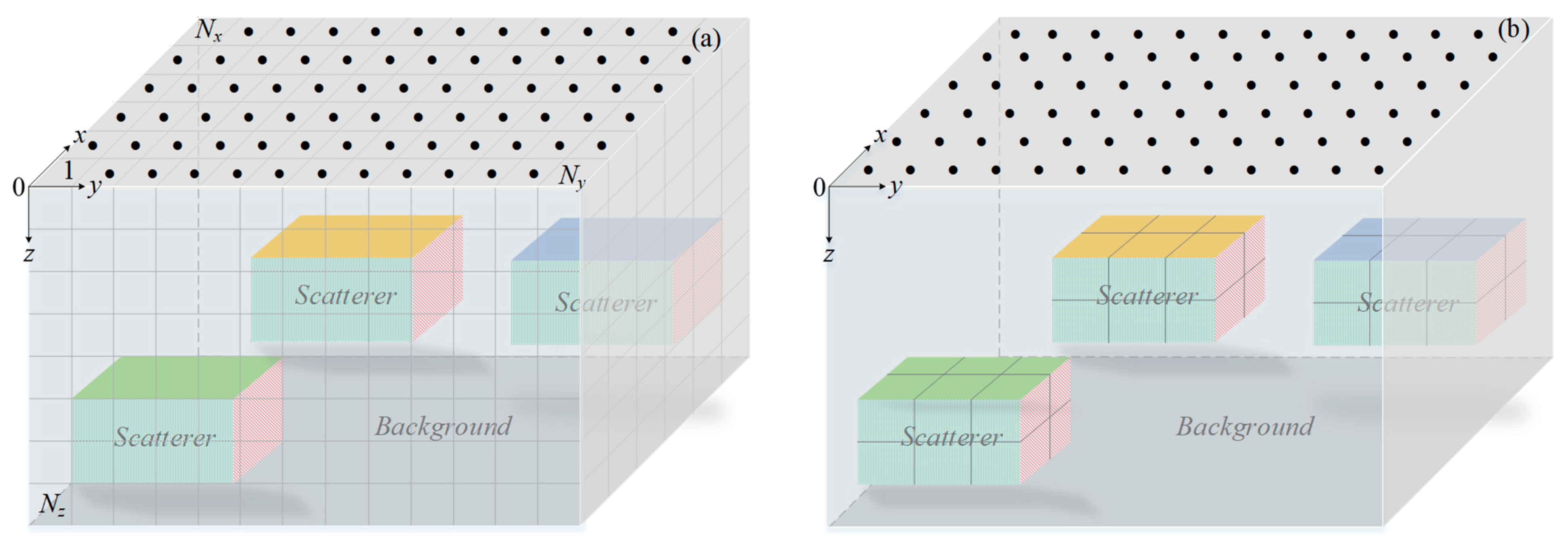
2. IE Method Foundation for MT Modeling

The procedure of MT modeling using the IE method has reached a fairly mature state [11,18,33,34,39]. We will not expound more than what is needed here. The governing equation of electric fields becomes

$$E\left(r\right)=E^{\mathrm{p}}\left(r\right)+{{\displaystyle \int }}_{v^{\prime }}{G}_E\left(r,r^{\prime }\right)\cdot J^{\mathrm{s}}\left(r\text{'}\right)\mathrm{d}v\text{'},$$

(1)

$$J^{\mathrm{s}}\left(r\text{'}\right)=\Delta \sigma E\left(r\prime \right),$$

(2)

where $E$ and $E^{\mathrm{p}}$ are the total and incident electric fields, respectively. $G_E$ is electrical dyadic Green’s function. $r$ and $r^{\prime }$ are coordinates related to observation points and sources, respectively. $v^{\prime }$ is the volume of the anomalous body, and $\Delta \sigma$ denotes the conductivity discrepancy between the abnormal body and half-space. Note that the electrical conductivity of the subsurface media is by nature characterized as a complex second order symmetric tensor [40,41,42]. This paper primarily exhibits a fast algorithm for MT forward modeling, and hence, only the real and isotropic conductivities are considered for simplicity. It is easy to take into account the anisotropy in the IE method by replacing the scalar conductivity in Equation (2) with a complex tensor, which does not increase the computational complexity. The complex and anisotropic conductivities will be considered in the future study.

To remain as the Toeplitz and Hankel matrices, Equation (1) is divided into three parts denoting three components of electric fields:

$${\mathit{E}}_x\left(r\right)={\mathit{E}}_x^{\mathrm{p}}\left(r\right)+{{\displaystyle \int }}_{v^{\prime }}\left[G_E^{xx}\left(r,r^{\prime }\right)J_x^{\mathrm{s}}\left(r\text{'}\right)+G_E^{xy}\left(r,r^{\prime }\right)J_y^{\mathrm{s}}\left(r\text{'}\right)+G_E^{xz}\left(r,r^{\prime }\right)J_z^{\mathrm{s}}\left(r\text{'}\right)\right]d{v}^{\prime },$$

(3)

$${\mathit{E}}_y\left(r\right)={\mathit{E}}_y^{\mathrm{p}}\left(r\right)+{{\displaystyle \int }}_{v^{\prime }}\left[G_E^{yx}\left(r,r^{\prime }\right)J_x^{\mathrm{s}}\left(r\text{'}\right)+G_E^{yy}\left(r,r^{\prime }\right)J_y^{\mathrm{s}}\left(r\text{'}\right)+G_E^{yz}\left(r,r^{\prime }\right)J_z^{\mathrm{s}}\left(r\text{'}\right)\right]d{v}^{\prime },$$

(4)

$${\mathit{E}}_z\left(r\right)={\mathit{E}}_z^{\mathrm{p}}\left(r\right)+{{\displaystyle \int }}_{v^{\prime }}\left[G_E^{zx}\left(r,r^{\prime }\right)J_x^{\mathrm{s}}\left(r\text{'}\right)+G_E^{zy}\left(r,r^{\prime }\right)J_y^{\mathrm{s}}\left(r\text{'}\right)+G_E^{zz}\left(r,r^{\prime }\right)J_z^{\mathrm{s}}\left(r\text{'}\right)\right]d{v}^{\prime },$$

(5)

Figure 1a shows a scattered domain comprising all anomalous bodies. Block cells are used to discretize the modeling domain with $N_x$, $N_y$ and $N_z$ cells in x-, y- and z-directions, respectively. Cells are numbered from left to right, front to back and up to down, while only anomalous bodies are discretized in Figure 1b. After discretization, Equation (3–5) can be written as:

$${\mathit{E}}_x\left(x,y,z\right)={\mathit{E}}_x^{\mathrm{p}}\left(x,y,z\right)+W_E^{xx}{J}_x^{\mathrm{s}}+W_E^{xy}{J}_y^{\mathrm{s}}+W_E^{xz}{J}_z^{\mathrm{s}},$$

(6)

$${\mathit{E}}_y\left(x,y,z\right)={\mathit{E}}_y^{\mathrm{p}}\left(x,y,z\right)+W_E^{yx}{J}_x^{\mathrm{s}}+W_E^{yy}{J}_y^{\mathrm{s}}+W_E^{yz}{J}_z^{\mathrm{s}},$$

(7)

$${\mathit{E}}_z\left(x,y,z\right)={\mathit{E}}_z^{\mathrm{p}}\left(x,y,z\right)+W_E^{zx}{J}_x^{\mathrm{s}}+W_E^{zy}{J}_y^{\mathrm{s}}+W_E^{zz}{J}_z^{\mathrm{s}},$$

(8)

where

$$W_E^{xx}={{\displaystyle \sum }}_{k=1}^{N_z}{{\displaystyle \sum }}_{j=1}^{N_y}{{\displaystyle \sum }}_{i=1}^{N_x}{{\displaystyle \int }}_{v_{ijk}}{G}_E^{xx}\left(x,y,z;\xi ,\eta ,\zeta \right)d\xi d\eta d\zeta ,$$

(9)

$$W_E^{xy}={{\displaystyle \sum }}_{k=1}^{N_z}{{\displaystyle \sum }}_{j=1}^{N_y}{{\displaystyle \sum }}_{i=1}^{N_x}{{\displaystyle \int }}_{v_{ijk}}{G}_E^{xy}\left(x,y,z;\xi ,\eta ,\zeta \right)d\xi d\eta d\zeta ,$$

(10)

$$W_E^{xz}={{\displaystyle \sum }}_{k=1}^{N_z}{{\displaystyle \sum }}_{j=1}^{N_y}{{\displaystyle \sum }}_{i=1}^{N_x}{{\displaystyle \int }}_{v_{ijk}}{G}_E^{xz}\left(x,y,z;\xi ,\eta ,\zeta \right)d\xi d\eta d\zeta ,$$

(11)

$$W_E^{yx}={{\displaystyle \sum }}_{k=1}^{N_z}{{\displaystyle \sum }}_{j=1}^{N_y}{{\displaystyle \sum }}_{i=1}^{N_x}{{\displaystyle \int }}_{v_{ijk}}{G}_E^{yx}\left(x,y,z;\xi ,\eta ,\zeta \right)d\xi d\eta d\zeta ,$$

(12)

$$W_E^{yy}={{\displaystyle \sum }}_{k=1}^{N_z}{{\displaystyle \sum }}_{j=1}^{N_y}{{\displaystyle \sum }}_{i=1}^{N_x}{{\displaystyle \int }}_{v_{ijk}}{G}_E^{yy}\left(x,y,z;\xi ,\eta ,\zeta \right)d\xi d\eta d\zeta ,$$

(13)

$$W_E^{yz}={{\displaystyle \sum }}_{k=1}^{N_z}{{\displaystyle \sum }}_{j=1}^{N_y}{{\displaystyle \sum }}_{i=1}^{N_x}{{\displaystyle \int }}_{v_{ijk}}{G}_E^{yz}\left(x,y,z;\xi ,\eta ,\zeta \right)d\xi d\eta d\zeta ,$$

(14)

$$W_E^{zx}={{\displaystyle \sum }}_{k=1}^{N_z}{{\displaystyle \sum }}_{j=1}^{N_y}{{\displaystyle \sum }}_{i=1}^{N_x}{{\displaystyle \int }}_{v_{ijk}}{G}_E^{zx}\left(x,y,z;\xi ,\eta ,\zeta \right)d\xi d\eta d\zeta ,$$

(15)

$$W_E^{zy}={{\displaystyle \sum }}_{k=1}^{N_z}{{\displaystyle \sum }}_{j=1}^{N_y}{{\displaystyle \sum }}_{i=1}^{N_x}{{\displaystyle \int }}_{v_{ijk}}{G}_E^{zy}\left(x,y,z;\xi ,\eta ,\zeta \right)d\xi d\eta d\zeta ,$$

(16)

$$W_E^{zz}={{\displaystyle \sum }}_{k=1}^{N_z}{{\displaystyle \sum }}_{j=1}^{N_y}{{\displaystyle \sum }}_{i=1}^{N_x}{{\displaystyle \int }}_{v_{ijk}}{G}_E^{zz}\left(x,y,z;\xi ,\eta ,\zeta \right)d\xi d\eta d\zeta ,$$

(17)

The $W$ in the Equations (9)–(17) can be divided into primary and secondary parts. The primary part, denoted as $W_E^{~\mathrm{p}}$, arises from subsurface currents and charges. The secondary part, denoted as $W_E^{~\mathrm{s}}$, arises from image currents and charges of earth-air interface, giving:

$$W_E^{~}=W_E^{~\mathrm{p}}+W_E^{~\mathrm{s}},$$

(18)

where the symbol ~ denotes components xx to zz.

Hohmann [33] has given an explicit form of the dyadic Green’s function, and we rewrite it in a form that makes it easier for readers to find the Toeplitz and Hankel matrices. A more explicit form of Equation (18) is:

$$W_E^{~}={{\displaystyle \sum }}_{k=1}^{N_z}{{\displaystyle \sum }}_{j=1}^{N_y}{{\displaystyle \sum }}_{i=1}^{N_x}{{\displaystyle \int }}_{v_{ijk}}{G}_E^{~}\left(x-\xi ,y-\eta ,z-\zeta \right)d\xi d\eta d\zeta +{{\displaystyle \sum }}_{k=1}^{N_z}{{\displaystyle \sum }}_{j=1}^{N_y}{{\displaystyle \sum }}_{i=1}^{N_x}{{\displaystyle \int }}_{v_{ijk}}{G}_E^{~}\left(x-\xi ,y-\eta ,z+\zeta \right)d\xi d\eta d\zeta ,$$

(19)

Three-level block Toeplitz matrix arises from the first part of the right-hand side in Equation (19) which is a translational invariant form, while the second part yields three-level block Toeplitz + Hankel matrices [43], namely, the first level is a Hankel matrix, and the second and third levels are Toeplitz matrices. In this study, the first level of these two kinds of matrices are $N_{zr}\times N_{zs}$ block matrices related to the number of electric field points and sources points in z-direction; analogously, the second level corresponds to x-direction, and the third level corresponds to y-direction. Taking the advantage of the block Toeplitz matrix, a matrix with constant diagonal elements, and the Hankel matrix, a matrix with constant anti-diagonal elements, we only need to compute and store non-redundant elements of the dense coefficient matrix. Specifically, the dense coefficient matrices $W_E^{xx\mathrm{p}}$, $W_E^{yy\mathrm{p}}$ and $W_E^{zz\mathrm{p}}$ in Equations (9), (13) and (17) are symmetric for each level. $W_E^{xy\mathrm{p}}$ is symmetric in the first level and antisymmetric in the second and third levels. $W_E^{xz\mathrm{p}}$ is symmetric in the third level and antisymmetric in the first and second levels. $W_E^{yz\mathrm{p}}$ is symmetric in the second level and antisymmetric in the first and third levels. $W_E^{yx\mathrm{p}}=W_E^{xy\mathrm{p}}$ , $W_E^{zx\mathrm{p}}=W_E^{xz\mathrm{p}}$, $W_E^{zy\mathrm{p}}=W_E^{yz\mathrm{p}}$. The matrices $W_E^{xx\mathrm{s}}$, $W_E^{yy\mathrm{s}}$ and $W_E^{zz\mathrm{s}}$ are symmetric for each level. $W_E^{xy\mathrm{s}}$ is symmetric in the first level and antisymmetric in the second as well as third levels. $W_E^{xz\mathrm{s}}$ is symmetric in the first and third levels while antisymmetric in the second level. $W_E^{yz\mathrm{s}}$ is symmetric in the first and second levels while antisymmetric in the third level. The symmetry and antisymmetry of matrices $W_E^{yx\mathrm{s}}$, $W_E^{zx\mathrm{s}}$ and $W_E^{zy\mathrm{s}}$ are in accord with $W_E^{xy\mathrm{s}}$, $W_E^{xz\mathrm{s}}$ and $W_E^{yz\mathrm{s}}$, respectively, but $W_E^{yx\mathrm{s}}\ne W_E^{xy\mathrm{s}}$, $W_E^{zx\mathrm{s}}\ne W_E^{xz\mathrm{s}}$, $W_E^{yz\mathrm{s}}\ne W_E^{zy\mathrm{s}}$. For symmetric and antisymmetric matrices, we just need to calculate the column or row of each level, namely, $N_x\times N_y\times N_z$ entities, and extend them to $\left(2N_x-1\right)\times \left(2N_y-1\right)\times \left(2N_z-1\right)$ before using 3-D FFT to calculate matrix-vector multiplication. Accordingly, the efficiency of computing coefficient matrices can be significantly improved compared with that of calculating the full matrices. For the discretization scheme in Figure 1a, more cells are required, but all EM fields at concerned positions can be obtained after solving the system of equations. It is also more suitable for inversion, since the amount of subsurface anomalous bodies is unknown. Although the case in Figure 1b calls for less cells, the structure of the coefficient matrix becomes more complicated. If one wants to use FFT for fast calculation, the matrix should be divided into Na×Na sub-matrices, where Na is the number of anomalous bodies. Sub-matrices represent interactions between each anomalous bodies, including self-interaction. Sub-matrices formed from self-interaction cases are square matrices, while others may be square or non-square matrices, which depends on the number of cells in each anomalous body. If the number of cells of two anomalous bodies are equivalent, the matrix is squared; otherwise, it is non-squared.

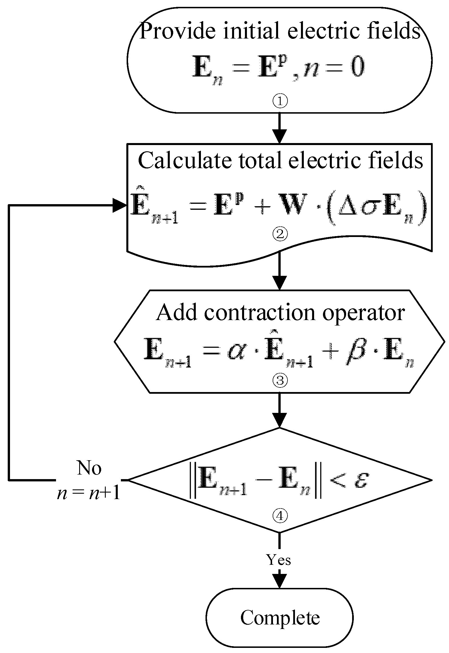
3. Improved Treatments

This section may be divided by subheadings. It should provide a concise and precise description of the experimental results, their interpretation, as well as the experimental conclusions that can be drawn.

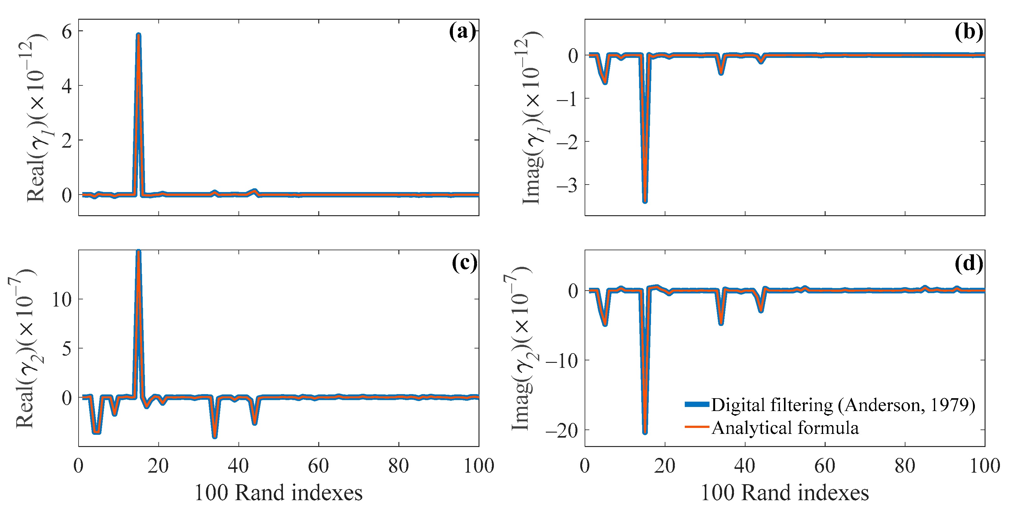
3.1. Analytical Method for Computation of Bessel Function

Another time-consuming factor when calculating coefficient matrices is two Bessel function integrals [33] that are relevant to the air–earth interface. They are given by:

$${\mathsf{𝜸}}_1=\frac{1}{4\mathsf{\pi }\mathrm{r}}{{\displaystyle \int }}_0^{\infty }\left(2-\frac{\mathsf{\lambda }}{{\mathrm{u}}_1}\right){\mathrm{e}}^{-{\mathrm{u}}_1\left(\mathrm{z}+{\mathrm{z}}^{\prime }\right)}{\mathrm{J}}_1\left(\mathsf{\lambda }\mathrm{r}\right)\mathsf{\lambda }\mathrm{d}\mathsf{\lambda },$$

(20)

$${\mathsf{𝜸}}_2=\frac{1}{4\mathsf{\pi }}{{\displaystyle \int }}_0^{\infty }\left(\frac{{\mathrm{u}}_1-\mathsf{\lambda }}{{\mathrm{u}}_1+\mathsf{\lambda }}\right)\frac{\mathsf{\lambda }}{{\mathrm{u}}_1}{\mathrm{e}}^{-{\mathrm{u}}_1\left(\mathrm{z}+{\mathrm{z}}^{\prime }\right)}{\mathrm{J}}_0\left(\mathsf{\lambda }\mathrm{r}\right)\mathrm{d}\mathsf{\lambda },$$

(21)

where $k_1=\sqrt{-i\omega {\mu }_0{\sigma }_b}$, $\omega$ is angular frequency, ${\mu }_0$ denotes magnetic permeability of free space, ${\sigma }_b$ is the conductivity of background earth, $u_1=\sqrt{{\lambda }^2-k_1^2}$. To fast compute the coefficient matrix, analytical formula instead of the digital filtering algorithm [44] are used to calculate Equations (20) and (21).

According to Sommerfeld integral

$${{\displaystyle \int }}_0^{\infty }\frac{\mathsf{\lambda }}{{\mathrm{u}}_1}{\mathrm{e}}^{-{\mathrm{u}}_1\left(\mathrm{z}+{\mathrm{z}}^{\prime }\right)}{\mathrm{J}}_0\left(\mathsf{\lambda }\mathrm{r}\right)\mathrm{d}\mathsf{\lambda }=\frac{{\mathrm{e}}^{-{\mathrm{ik}}_1{\mathrm{R}}_{\mathrm{s}}}}{{\mathrm{R}}_{\mathrm{s}}},$$

(22)

and the integral

$${{\displaystyle \int }}_0^{\infty }\frac{1}{{\mathrm{u}}_1}{\mathrm{e}}^{-{\mathrm{u}}_1\left(\mathrm{z}+{\mathrm{z}}^{\prime }\right)}{\mathrm{J}}_0\left(\mathsf{\lambda }\mathrm{r}\right)\mathrm{d}\mathsf{\lambda }={\mathrm{I}}_0\left(\mathrm{P}\right){\mathrm{K}}_0\left(\mathrm{Q}\right),$$

(23)

we can obtain the analytical formula of ${𝜸}_1$ and ${𝜸}_2$  [45,46] (see Appendix A)

$${𝜸}_1=\frac{1}{4{\mathsf{\pi }\mathrm{R}}_{\mathrm{s}}^3}\left(2{\mathsf{\theta }}_1-{\mathrm{e}}^{-{\mathrm{ik}}_1{\mathrm{R}}_{\mathrm{s}}}-{\mathrm{ik}}_1{\mathrm{R}}_{\mathrm{s}}{\mathrm{e}}^{-{\mathrm{ik}}_1{\mathrm{R}}_{\mathrm{s}}}\right).$$

(24)

where ${\theta }_1=P{I}_1{K}_0+Q{I}_0{K}_1-h\left(I_0{K}_0-I_1{K}_1\right)$, $h=k_1^2{R}_s\left(z+z^{\prime }\right)/2$, $P=i{k}_1\left[R_s-\left(z+z^{\prime }\right)\right]/2$, $Q=i{k}_1\left[R_s+\left(z+z^{\prime }\right)\right]/2$.

In addition,

$${𝜸}_2=\frac{1}{4\mathsf{\pi }}\left\{\frac{2}{{\mathrm{k}}_1^2}\left(2{\mathrm{S}}_1-{\mathrm{S}}_2\right)-\frac{2\mathsf{\beta }}{{\mathrm{k}}_1^2{\mathrm{R}}_{\mathrm{s}}^2}\left[{\mathsf{\tau }}_1-\frac{{\left(\mathrm{z}+{\mathrm{z}}^{\prime }\right)}^2{\mathsf{\tau }}_2}{{\mathrm{R}}_{\mathrm{s}}^2}\right]+\mathsf{\beta }\right\},$$

(25)

where ${\tau }_1=i{k}_1{R}_s+1$, ${\tau }_2=3i{k}_1{R}_s-k_1^2{R}_s^2+3$, $\beta =-\frac{e^{-i{k}_1{R}_s}}{R_s}$, $S_1=\frac{{\theta }_1}{R_s^3}$, $S_2=\frac{3r^2{\theta }_1-R_s^2{\theta }_2}{R_s^5}$, ${\theta }_2=h\left[g\left(I_0{K}_1-I_1{K}_0\right)-2I_1{K}_1\right]$, $g=i{k}_1{r}^2/R_s$. $I_n$ and $K_n$ are the first and second kind modified Bessel functions for order $n$ with variables $P$ and $Q$, respectively, which can be solved by polynomial approximation [47].

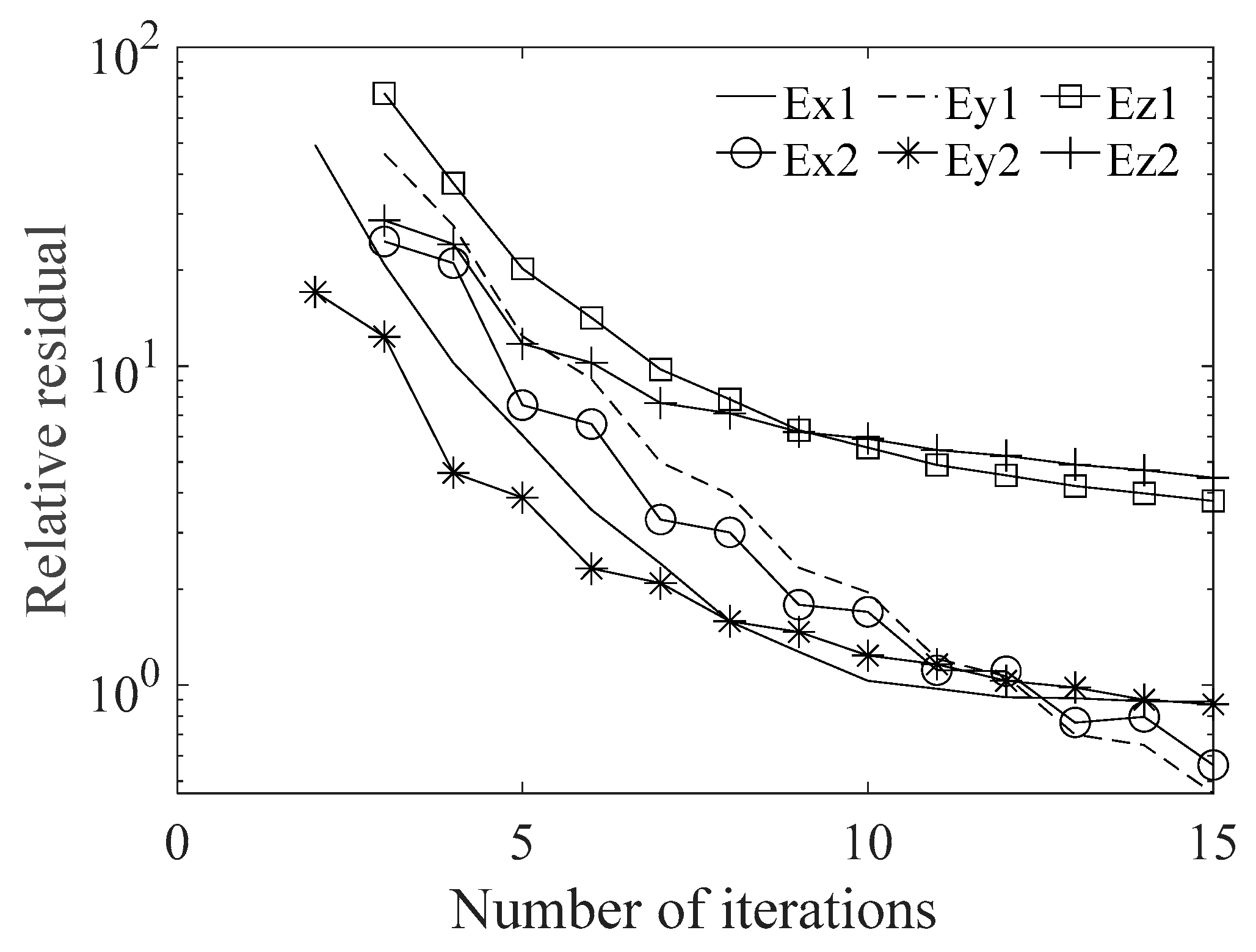
3.2. Rapid Implementation of Coefficient Matrix-Vector Multiplication

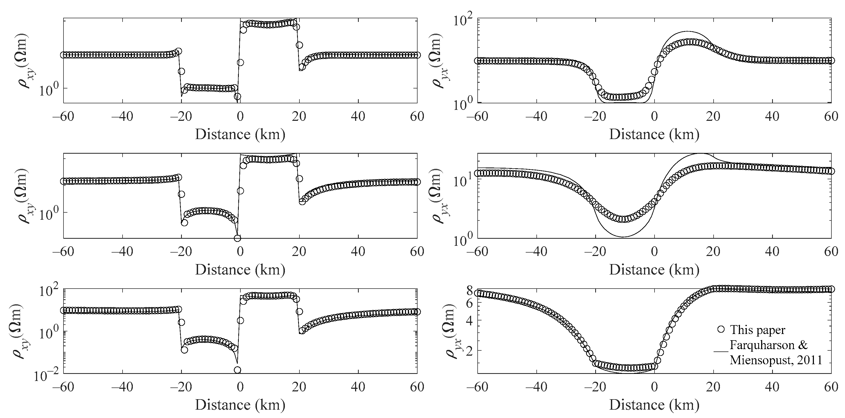
According to the aforementioned special matrices, we are able to implement fast calculation of matrix-vector multiplication using 3-D FFT. In order to use FFT, the Toeplitz + Hankel matrix needs to be transformed into a Toeplitz matrix as follows:

$$Hx=\left[\begin{array}{ccc}{h}_3& h_2& h_1\\ h_2& h_1& h_4\\ h_1& h_4& h_5\end{array}\right]\left[\begin{array}{c}{x}_1\\ x_2\\ x_3\end{array}\right]\stackrel{\begin{array}{c}\mathrm{reverse} \mathrm{the} \mathrm{columns} \mathrm{order} \mathrm{and} \mathrm{rows} \mathrm{order}\\ \mathrm{of} \mathrm{the} \mathrm{matrix} \mathrm{and} \mathrm{vector}, \mathrm{respectively}\\ \end{array}}{\iff }\left[\begin{array}{ccc}{h}_1& h_2& h_3\\ h_4& h_1& h_2\\ h_5& h_4& h_1\end{array}\right]\left[\begin{array}{c}{x}_3\\ x_2\\ x_1\end{array}\right]=T{x}^{\mathrm{R}}.$$

(26)

Only the first level of the Toeplitz + Hankel matrix needs to be transformed into a Toeplitz matrix in the case of this study. Subsequently, as for submatrices formed from self-interaction of anomalous bodies, we can reconstruct the coefficient matrix following the approach applied to gravity modeling [37] by changing 2-D FFT to 3-D FFT, which described the procedures to rearrange the coefficient matrix in detail. For submatrices of interaction of different anomalous bodies that method is not available anymore. If we use the discretization scheme in Figure 1a, that method still works. In the following sections, we focus on the discretization scheme shown in Figure 1b. To be adequate to all submatrices mentioned above, we presented a new method to reconstruct the non-redundant values of the full matrix as follows. Suppose we have a random 3-level asymmetric Toeplitz matrix

$$\mathbf{A}=\left[\begin{array}{cccccccccccc}1& 2& 3& 3& 8& 9& 7& 8& 4& 9& 2& 1\\ 3& 1& 2& 2& 3& 8& 2& 7& 8& 5& 9& 2\\ 5& 3& 1& 0& 2& 3& 5& 2& 7& 0& 5& 9\\ 2& 4& 5& 1& 2& 3& 8& 4& 3& 7& 8& 4\\ 6& 2& 4& 3& 1& 2& 1& 8& 4& 2& 7& 8\\ 7& 6& 2& 5& 3& 1& 7& 1& 8& 5& 2& 7\\ 4& 3& 1& 6& 7& 4& 1& 2& 3& 3& 8& 9\\ 4& 4& 3& 3& 6& 7& 3& 1& 2& 2& 3& 8\\ 0& 4& 4& 5& 3& 6& 5& 3& 1& 0& 2& 3\\ 5& 2& 1& 4& 3& 1& 2& 4& 5& 1& 2& 3\\ 7& 5& 2& 4& 4& 3& 6& 2& 4& 3& 1& 2\\ 4& 7& 5& 0& 4& 4& 7& 6& 2& 5& 3& 1\end{array}\right],$$

(27)

and a random vector

$$x={\left[\begin{array}{cccccccccccc}1& 2& 3& 4& 5& 6& 7& 8& 9& 10& 11& 12\end{array}\right]}^{\mathrm{T}}.$$

(28)

We only need to calculate the following non-redundant values of matrix A and sort them in a 3-D array

$$a\left(:,:,1\right)=\left[\begin{array}{c}\begin{array}{ccc}4& 7& \begin{array}{ccc}5& 2& 1\end{array}\end{array}\\ \begin{array}{ccc}0& 4& \begin{array}{ccc}4& 3& 1\end{array}\end{array}\\ \begin{array}{ccc}5& 3& \begin{array}{ccc}6& 7& 4\end{array}\end{array}\end{array}\right],a\left(:,:,2\right)=\left[\begin{array}{c}\begin{array}{ccc}7& 6& \begin{array}{ccc}2& 4& 5\end{array}\end{array}\\ \begin{array}{ccc}5& 3& \begin{array}{ccc}1& 2& 3\end{array}\end{array}\\ \begin{array}{ccc}0& 2& \begin{array}{ccc}3& 8& 9\end{array}\end{array}\end{array}\right],a\left(:,:,3\right)=\left[\begin{array}{c}\begin{array}{ccc}7& 1& \begin{array}{ccc}8& 4& 3\end{array}\end{array}\\ \begin{array}{ccc}5& 2& \begin{array}{ccc}7& 8& 4\end{array}\end{array}\\ \begin{array}{ccc}0& 5& \begin{array}{ccc}9& 2& 1\end{array}\end{array}\end{array}\right],$$

(29)

After zero padding, the format of vector x is

$$x\left(:,:,1\right)=\left[\begin{array}{c}\begin{array}{ccc}12& 11& \begin{array}{ccc}10& 0& 0\end{array}\end{array}\\ \begin{array}{ccc}9& 8& \begin{array}{ccc}7& 0& 0\end{array}\end{array}\\ \begin{array}{ccc}0& 0& \begin{array}{ccc}0& 0& 0\end{array}\end{array}\end{array}\right], x\left(:,:,2\right)=\left[\begin{array}{c}\begin{array}{ccc}6& 5& \begin{array}{ccc}4& 0& 0\end{array}\end{array}\\ \begin{array}{ccc}3& 2& \begin{array}{ccc}1& 0& 0\end{array}\end{array}\\ \begin{array}{ccc}0& 0& \begin{array}{ccc}0& 0& 0\end{array}\end{array}\end{array}\right], x\left(:,:,3\right)=\left[\begin{array}{c}\begin{array}{ccc}0& 0& \begin{array}{ccc}0& 0& 0\end{array}\end{array}\\ \begin{array}{ccc}0& 0& \begin{array}{ccc}0& 0& 0\end{array}\end{array}\\ \begin{array}{ccc}0& 0& \begin{array}{ccc}0& 0& 0\end{array}\end{array}\end{array}\right],$$

(30)

Compared with the method of Vogel [48] and Chen and Liu [37], we need no more extra zeros to pad array a. Using the discrete convolution theorem

$$f=\mathrm{ifftn}\left[\mathrm{fftn}\left(a\right)\cdot \mathrm{fftn}\left(x\right)\right],$$

(31)

here $\mathrm{fftn}$ and $\mathrm{ifftn}$ denote 3-D FFT and inverse 3-D FFT, respectively. The sign $\cdot$ is the dot product operator. Extracting values from $f$ in Equation (31), one can obtain the desired solutions. For the non-square matrix, an identical matrix-vector multiplication procedure can be used.

The successive iterative method or Born series [27,32,49] is used to solve Equations (6)–(8), and the fast algorithm above can be used to speed up matrix-vector multiplication at each iteration. In consideration of the convergence of the iterative method for large conductivity contrast and large size models, the contraction operator established by Zhdanov and Fang [32] needs to be added to Equations (6)–(8) during each iteration, as shown in the following flow chart.

Neglecting displacement currents, the contraction operator $\alpha$ and $\beta$ in Figure 2 are as follows:

$$\alpha =\frac{2{\sigma }_b}{2{\sigma }_b+\Delta \sigma },\beta =\frac{\Delta \sigma }{2{\sigma }_b+\Delta \sigma }.$$

(32)

Consequently, magnetic fields can be obtained by taking the curl of the solved electric fields following Hohmann [33].

4. Model Test

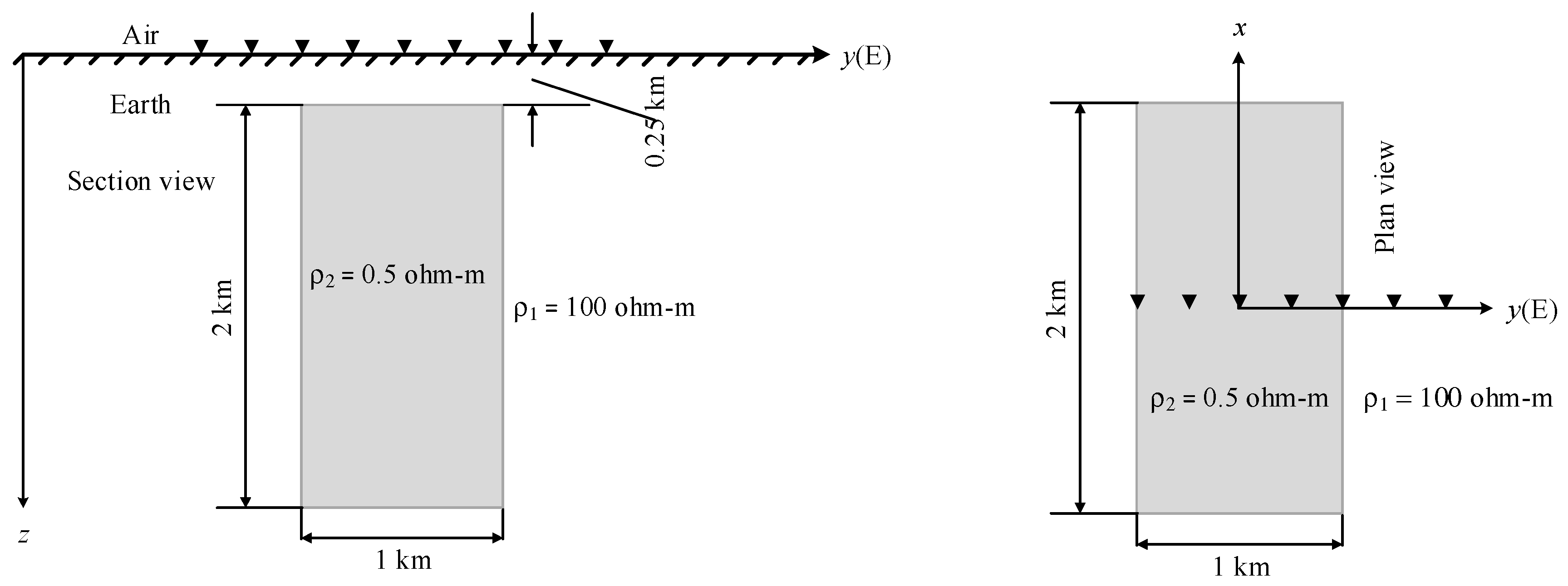
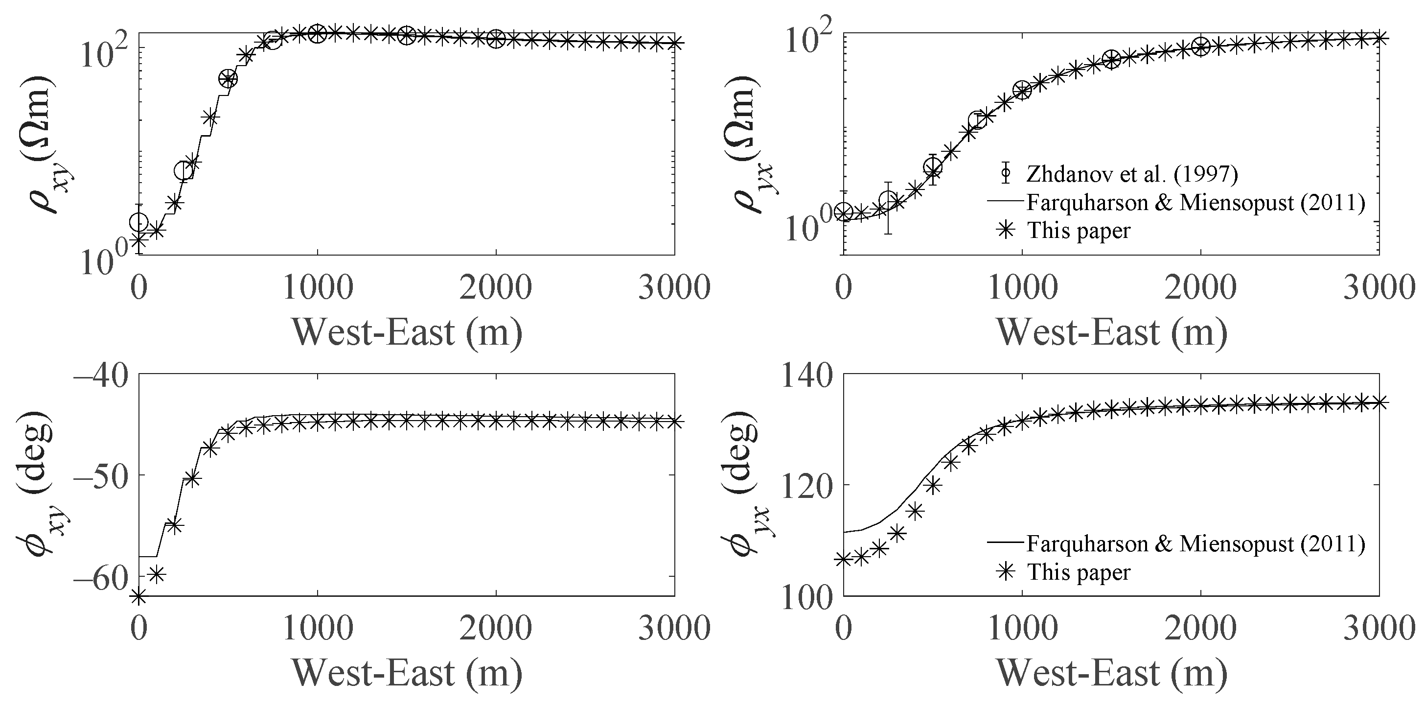
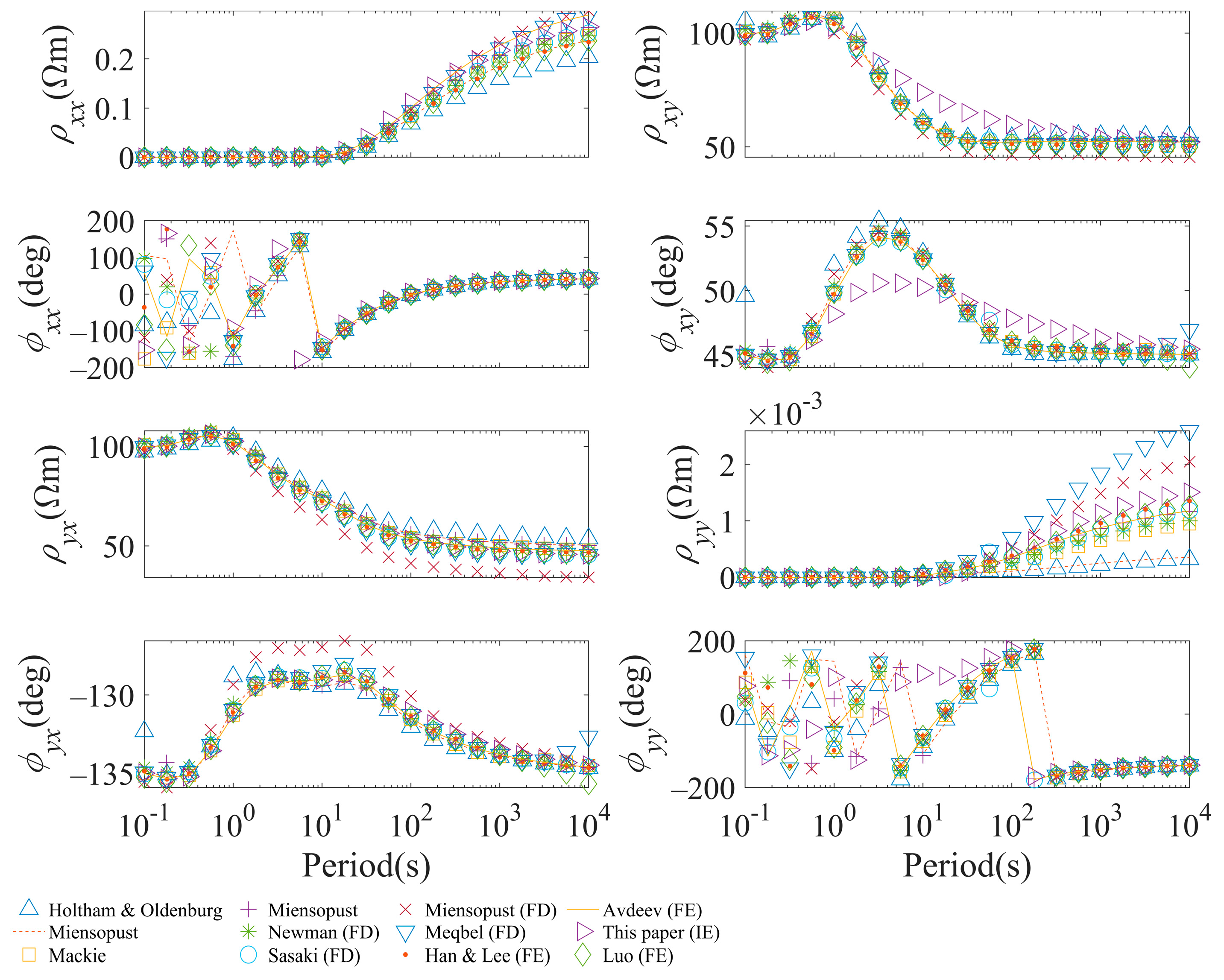
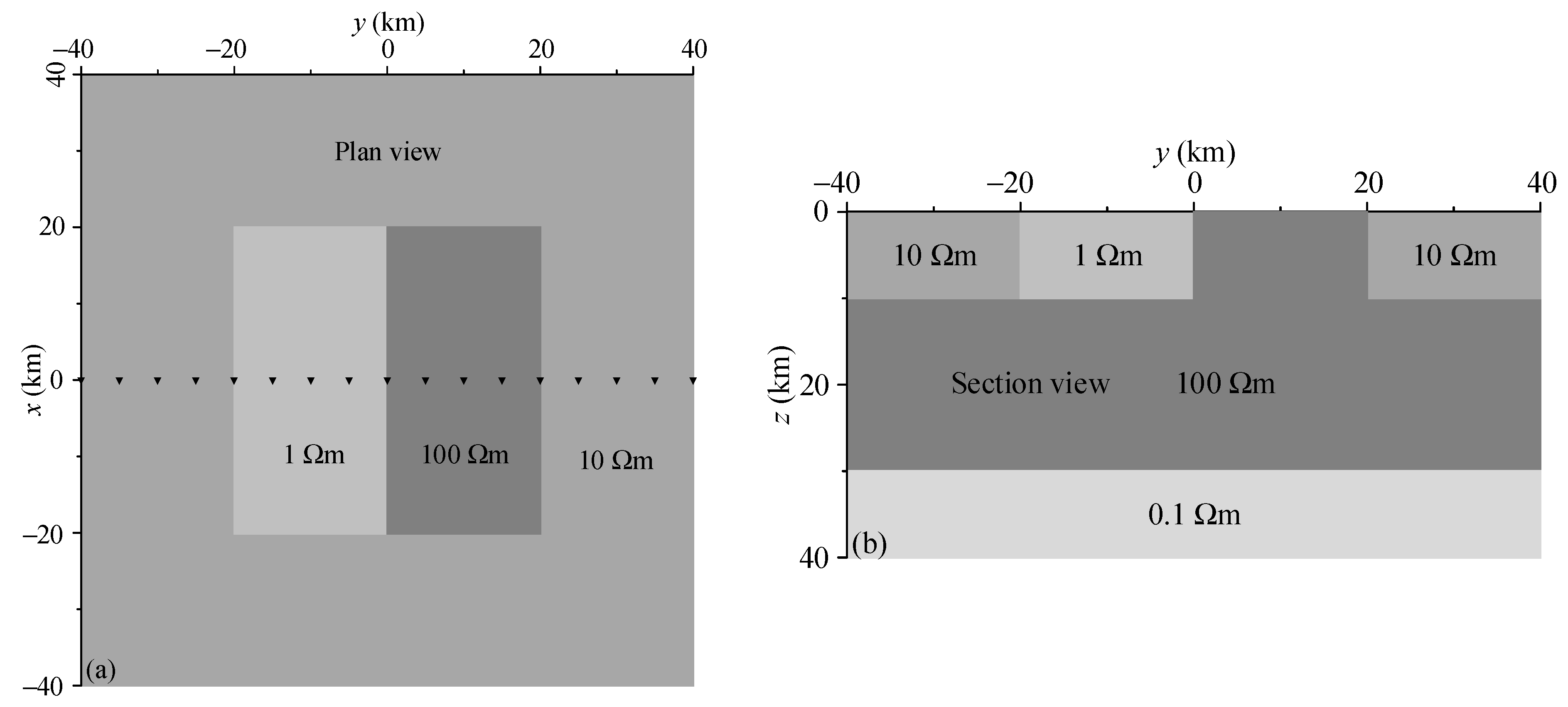
4.1. COMMEMI 3D-1A Model

The COMMEMI 3D-1A model (Figure 3) with a large contrast in conductivity (${\rho }_1/{\rho }_2=200$) [50] is used to validate our developed IE solver. We discretize the anomalous body into $20\times 10\times 20$ cells with size $100\mathrm{m}\times 100\mathrm{m}\times 100\mathrm{m}$ in x-, y- and z-directions, respectively. Apparent resistivity and phase for 0.1 Hz after 10 iterations are shown in Figure 4. Using MATLAB R2019b (The MathWorks, Inc., Natick, MA, USA), it cost the CPU time 1.3 s and a little RAM based on a ThinkPad P50 Mobile Workstation Laptop (Lenovo, Beijing, China) with basic specifications (3.5 GHz Intel Core i7 processor (Intel Corporation, Santa Clara, CA, USA), 64 GB RAM). Figure 4 shows that our results agree well with the results of previous papers [5,50] with a small number of discretization cells and low computational cost. Figure 5 presents the convergence of successive iteration approach when solving electric fields.

In this part, we compare the accuracy and efficiency of calculating ${𝜸}_1$ and ${𝜸}_2$ in Equations (20) and (21) using the digital filtering method [44] as well as the analytical formulas described in Equations (24) and (25). It is meaningless to compare the computational cost of ${𝜸}_1$ and ${𝜸}_2$ for one cell. Hence, we divide COMMEMI 3D-1A into 50 × 50 × 50 cells in the x-, y- and z-direction, respectively, which implies $\left(2\times 50-1\right)\times \left(2\times 50-1\right)\times \left(2\times 50-1\right)=970,299$ entities to be calculated. It costs 39.0 s and 61.3 s to calculate ${𝜸}_1$, ${𝜸}_2$, respectively, by digital filtering methods. While they are merely 0.85 s and 0.89 s through analytical formulas. Figure 6 shows 100 random real and imaginary parts of ${𝜸}_1$ and ${𝜸}_2$ among 970,299 entities by the two methods. They are practically identical with each other. Making use of the analytical formula can remarkably decrease the time of calculating ${𝜸}_1$ and ${𝜸}_2$ especially for plenty of cells.

4.2. Dublin Test Model 1

In this part, the Dublin Test Model (MTNet-Home, https://www.mtnet.info/main/ (accessed on 15 March 2022)) provided at the MT 3D inversion workshop in Dublin is used to test the applicability of the presented algorithm to complex conductivity structures. The model is composed of three different blocks in a homogeneous $100\mathsf{\Omega }\mathrm{m}$ half-space with the largest contrast in resistivity of 10,000/1. The sizes, locations and resistivities of three anomalous bodies are shown in Figure 7 and

Table 1. The size and resistivity of anomalous bodies.

	Extend in x (km)	Extend in y (km)	Extend in z (km)	$\mathbf{Resistivity}\left(\mathbf{\Omega }\mathbf{m}\right)$
Block 1	−20 to 20	−2.5 to 2.5	5 to 20	10
Block 2	−15 to 0	−2.5 to 22.5	20 to 25	1
Block 3	0 to 15	−22.5 to 2.5	20 to 50	10,000

. We use cubic cells to discretize the three anomalous domains into $40\times 5\times 15$, $15\times 25\times 5$ and $15\times 25\times 30$ cells in the x-, y- and z-directions, respectively. With 21 periods ranging from 0.1 s to 10,000 s, we compare our apparent resistivity with those provided by Miensopust et al. [51], which includes results of 11 codes. We choose 2–11 results for comparison because the first result shows a big difference with others. In addition, the result of edge-based finite element [52] denoted as green rhombus is also used for comparison. As shown in Figure 8, all apparent resistivity and phase components, xx, xy, yx and yy, at the observational site (0, 0, 0) m after 30 iterations are closed to most of the 11 results, and the time consumption is about 25 s per period. The relative residual norms between two adjacent successive iterations for different periods are shown in Figure 9, which shows the good convergence rate of this iterative method. This example shows that our algorithm is able to solve the complex and high contrast of electrical conductivity structures efficiently.

In order to test the time and memory consumption of the presented algorithm, four discretization strategies shown in

Table 2. Time and memory consumption for different cells.

Computation Cost			Number of Cells in x-, y-, z-Direction for Anomalous Bodies
Iterations	Time (s)/Period	Peak RAM(GB)	Body 1	Body 2	Body 3
30	25	0.047	$40\times 5\times 15$	$15\times 25\times 5$	$15\times 25\times 30$
20	108	0.2	$64\times 8\times 24$	$24\times 40\times 8$	$24\times 40\times 48$
20	234	0.4	$80\times 10\times 30$	$30\times 50\times 10$	$30\times 50\times 60$
20	2061	3.19	$160\times 20\times 60$	$60\times 100\times 20$	$60\times 100\times 120$

are carried out for the DTM1 model. Solutions of apparent resistivities are consistent with those shown in Figure 8 and are not presented here. This experiment shows the capacity of our algorithm to solve millions of cells with acceptable time and memory use.

4.3. COMMEMI 3D-2A Model

The COMMEMI 3D-2A [50] model comprising a three-layer background is used to test that our algorithm is adequate to model layered-Earth in this section. There are two anomalous prisms embedded in the top layer as shown in Figure 10. In order to use simpler half-space Green’s function compared with layered Green’s function, we treat the layered-Earth as anomalous bodies. We compared our results with the FE values of Farquharson and Miensopust [5]. The compared apparent resistivities for 0.1, 0.01 and 0.001 Hz are shown in Figure 11, and they agree well with each other. In this way, it indeed requires more discretized cells; however, we can calculate the responses of models with layered background using the half-space Green’s function. Consequently, the aforementioned algorithms that analytical computation of Bessel function integrals and fast calculation of matrix-vector multiplication can be exploited. In theory, the layered background should be infinitely extended in the horizontal direction, but the amplitude of secondary fields induced by anomalous bodies will be exponentially reduced to zero due to the skin effect. Thus, we can choose the appropriate horizontal extension of layered-Earth as background instead of infinite extension. Moreover, the layered-Earth does not always stretch far horizontally and continuously in realistic geologic earth, therefore, it is reasonable to take layered-Earth as anomalous bodies.

5. Discussion

For a layered-Earth background, such as the COMMEMI 3D-2A model, the layered media Green’s function is more suitable for the IE method. However, the expressions of the layered media Green’s function are more complicated compared with the half-space case. There are two significant differences in their IE implementation. Firstly, the coefficient matrices resulting from discretizing the IE equation exhibit different structures. The matrices in the layered media case can be divided into two parts. One part is related to the direct wave from the whole space, namely, when the observational points and scatter sources are at the same background layers. For this part, the structure of the matrices is identical with the primary part $W_E^{~\mathrm{p}}$ in Equation (18) of the half-space case, they are symmetric or antisymmetric three-level Toeplitz matrices, while the other part is related to the reflected wave from different layers. Different from the half-space case, these matrices are not three-level Toeplitz + Hankel matrices, but they are two-level Toeplitz matrices when the observational points and scatter sources are at the same discretized layers, and one can use 2-D FFT to conduct matrix-vector multiplication for this case. It requires $N_z^2$ times 2-D FFT and is more time-consuming compared with the half-space case. Secondly, it is hard to find the analytical formulas for the Bessel function integral in layered media case as we do in the half-space case. As a result, the digital filtering method has to be used for calculating the Bessel function integral which significantly increases the computational time.

For the coefficient matrices with a different structure in the layered media case, we have developed corresponding efficient algorithms to conduct matrix-vector multiplication, but this is beyond the scope of this study and will be discussed in detail in future work.

6. Conclusions

This study presents a fast algorithm to solve MT modeling based on the IE method. To improve computational efficiency, an analytical formula is used to calculate the integral of the Bessel function in the Green’s function. Coefficient matrices are symmetric and antisymmetric, three-level block-Toeplitz and Toeplitz + Hankel matrices owing to the translational invariance and convolutional nature of the free-space Green’s function. Taking advantage of this special matrix structure, we simply calculate and store $N_x\times N_y\times N_z$ entities and extend them to $\left(2N_x-1\right)\times \left(2N_y-1\right)\times \left(2N_z-1\right)$ entities before using 3-D FFT to calculate the matrix-vector multiplication. Afterward, we construct these non-redundant entities into a well-organized array and use 3-D FFT to compute matrix-vector multiplication efficiently at each iteration. Conventional IE method is difficult to solve a large and complex modeling region due to the preceding obstacles. This study makes the IE method a more powerful numerical approach to electromagnetic modeling.

References

1. Dong, S.; Li, T.; Chen, X.; Zhou, Q.; Liu, Z.; Zhang, J. The Updated Progress of SinoProbe—Deep Exploration in China. In Proceedings of the AGU Fall Meeting Abstracts, San Francisco, CA, USA, 5–9 December 2011; p. T53E-01. [Google Scholar]
2. Meqbel, N.M.; Egbert, G.D.; Wannamaker, P.E.; Kelbert, A.; Schultz, A. Deep electrical resistivity structure of the northwestern U.S. derived from 3-D inversion of USArray magnetotelluric data. Earth Planet. Sci. Lett. 2014, 402, 290–304. [Google Scholar] [CrossRef]
3. Clowes, R.; Cook, F.; Hajnal, Z.; Hall, J.; Lewry, J.; Lucas, S.; Wardle, R. Canada’s LITHOPROBE Project (Collaborative, multidisciplinary geoscience research leads to new understanding of continental evolution). Episodes 1999, 22, 3–20. [Google Scholar] [CrossRef] [Green Version]
4. Thiel, S.; Goleby, B.R.; Pawley, M.J.; Heinson, G. AusLAMP 3D MT imaging of an intracontinental deformation zone, Musgrave Province, Central Australia. Earth Planets Space 2020, 72, 98. [Google Scholar] [CrossRef]
5. Farquharson, C.G.; Miensopust, M.P. Three-dimensional finite-element modelling of magnetotelluric data with a divergence correction. J. Appl. Geophys. 2011, 75, 699–710. [Google Scholar] [CrossRef]
6. Varılsüha, D. 3D inversion of magnetotelluric data by using a hybrid forward-modeling approach and mesh decoupling. Geophysics 2020, 85, E191–E205. [Google Scholar] [CrossRef]
7. Yin, C.; Zhang, B.; Liu, Y.; Cai, J. A goal-oriented adaptive finite-element method for 3D scattered airborne electromagnetic method modeling. Geophysics 2016, 81, E337–E346. [Google Scholar] [CrossRef]
8. Jahandari, H.; Farquharson, C.G. A finite-volume solution to the geophysical electromagnetic forward problem using unstructured grids. Geophysics 2014, 79, E287–E302. [Google Scholar] [CrossRef]
9. Avdeev, D.B. Three-Dimensional Electromagnetic Modelling and Inversion from Theory to Application. Surv. Geophys. 2005, 26, 767–799. [Google Scholar] [CrossRef]
10. Varilsüha, D.; Candansayar, M.E. 3D magnetotelluric modeling by using finite-difference method: Comparison study of different forward modeling approaches. Geophysics 2018, 83, WB51–WB60. [Google Scholar] [CrossRef]
11. Berdichevsky, M.N.; Dmitriev, V.I. Models and Methods of Magnetotellurics; Springer: Berlin, Germany, 2008; pp. 350–351. [Google Scholar] [CrossRef]
12. Ansari, S.; Schetselaar, E.; Craven, J.; Farquharson, C. Three-dimensional magnetotelluric numerical simulation of realistic geologic models. Geophysics 2020, 85, E171–E190. [Google Scholar] [CrossRef]
13. Cai, H.; Long, Z.; Lin, W.; Li, J.; Lin, P.; Hu, X. 3D multinary inversion of controlled-source electromagnetic data based on the finite-element method with unstructured mesh. Geophysics 2020, 86, E77–E92. [Google Scholar] [CrossRef]
14. Lu, X.; Farquharson, C.G. 3D finite-volume time-domain modeling of geophysical electromagnetic data on unstructured grids using potentials. Geophysics 2020, 85, E221–E240. [Google Scholar] [CrossRef]
15. Jahandari, H.; Farquharson, C.G. Finite-volume modelling of geophysical electromagnetic data on unstructured grids using potentials. Geophys. J. Int. 2015, 202, 1859–1876. [Google Scholar] [CrossRef]
16. Barnett, A.H.; Magland, J.; af Klinteberg, L. A Parallel Nonuniform Fast Fourier Transform Library Based on an “Exponential of Semicircle” Kernel. SIAM J. Sci. Comput. 2019, 41, C479–C504. [Google Scholar] [CrossRef]
17. Ren, Z.; Chen, C.; Tang, J.; Zhou, F.; Chen, H.; Qiu, L.; Shuanggui, H. A new integral equation approach for 3D MT modeling. Chin. J. Geophys. 2017, 60, 4506–4515. [Google Scholar] [CrossRef]
18. Zhdanov, M.; Lee, S.K.; Yoshioka, K. Integral equation method for 3D modeling of electromagnetic fields in complex structures with inhomogeneous background conductivity. Geophysics 2006, 71, G333–G345. [Google Scholar] [CrossRef]
19. Everett, M.E. Theoretical Developments in Electromagnetic Induction Geophysics with Selected Applications in the Near Surface. Surv. Geophys. 2012, 33, 29–63. [Google Scholar] [CrossRef]
20. Avdeev, D.; Knizhnik, S. 3D integral equation modeling with a linear dependence on dimensions. Geophysics 2009, 74, F89–F94. [Google Scholar] [CrossRef]
21. Nishimura, N. Fast multipole accelerated boundary integral equation methods. Appl. Mech. Rev. 2002, 55, 299–324. [Google Scholar] [CrossRef]
22. Rokhlin, V. Rapid solution of integral equations of classical potential theory. J. Comput. Phys. 1985, 60, 187–207. [Google Scholar] [CrossRef]
23. Schobert, D.T.; Eibert, T.F. Fast Integral Equation Solution by Multilevel Green’s Function Interpolation Combined With Multilevel Fast Multipole Method. IEEE Trans. Antennas Propag. 2012, 60, 4458–4463. [Google Scholar] [CrossRef]
24. Beylkin, G.; Coifman, R.; Rokhlin, V. Fast wavelet transforms and numerical algorithms I. Commun. Pure Appl. Math. 1991, 44, 141–183. [Google Scholar] [CrossRef]
25. Kim, H.; Ling, H. On the application of fast wavelet transform to the integral-equation solution of electromagnetic scattering problems. Microw. Opt. Technol. Lett. 1993, 6, 168–173. [Google Scholar] [CrossRef]
26. Canning, F.X. Improved impedance matrix localization method (EM problems). IEEE Trans. Antennas Propag. 1993, 41, 659–667. [Google Scholar] [CrossRef]
27. Hursán, G.; Zhdanov, M.S. Contraction integral equation method in three-dimensional electromagnetic modeling. Radio Sci. 2002, 37, 1–13. [Google Scholar] [CrossRef] [Green Version]
28. Singer, B.S. Electromagnetic integral equation approach based on contraction operator and solution optimization in Krylov subspace. Geophys. J. Int. 2008, 175, 857–884. [Google Scholar] [CrossRef] [Green Version]
29. Pankratov, O.; Kuvshinov, A. Applied Mathematics in EM Studies with Special Emphasis on an Uncertainty Quantification and 3-D Integral Equation Modelling. Surv. Geophys. 2016, 37, 109–147. [Google Scholar] [CrossRef]
30. Singer, B.S. Method for solution of Maxwell’s equations in non-uniform media. Geophys. J. Int. 1995, 120, 590–598. [Google Scholar] [CrossRef]
31. Pankratov, O.; Avdeev, D.; Kuvshinov, A. Electromagnetic field scattering in a heterogeneous Earth: A solution to the forward problem. Phys. Solid Earth 1995, 31, 201–209. [Google Scholar]
32. Zhdanov, M.S.; Fang, S. Quasi-linear series in three-dimensional electromagnetic modeling. Radio Sci. 1997, 32, 2167–2188. [Google Scholar] [CrossRef] [Green Version]
33. Hohmann, G.W. Three-Dimensional Induced Polarization and Electromagnetic Modeling. Geophysics 1975, 40, 309–324. [Google Scholar] [CrossRef]
34. Wannamaker, P.; Hohmann, G.; San Filipo, W. Electromagnetic modeling of three-dimensional bodies in layered earths using integral equations. Geophysics 1984, 49, 60–74. [Google Scholar] [CrossRef]
35. Wannamaker, P.E. Advances in three-dimensional magnetotelluric modeling using integral equations. Geophysics 1991, 56, 1716–1728. [Google Scholar] [CrossRef]
36. Zhdanov, M.S.; Wan, L.; Gribenko, A.; Čuma, M.; Key, K.; Constable, S. Large-scale 3D inversion of marine magnetotelluric data: Case study from the Gemini prospect, Gulf of Mexico. Geophysics 2011, 76, F77–F87. [Google Scholar] [CrossRef]
37. Chen, L.; Liu, L. Fast and accurate forward modelling of gravity field using prismatic grids. Geophys. J. Int. 2019, 216, 1062–1071. [Google Scholar] [CrossRef]
38. Kamm, J.; Pedersen, L.B. Inversion of airborne tensor VLF data using integral equations. Geophys. J. Int. 2014, 198, 775–794. [Google Scholar] [CrossRef] [Green Version]
39. Ting, S.C.; Hohmann, G.W. Integral equation modeling of three-dimensional magnetotelluric response. Geophysics 1981, 46, 182–197. [Google Scholar] [CrossRef] [Green Version]
40. Abdulsamad, F.; Revil, A.; Ghorbani, A.; Toy, V.; Kirilova, M.; Coperey, A.; Duvillard, P.A.; Ménard, G.; Ravanel, L. Complex Conductivity of Graphitic Schists and Sandstones. J. Geophys. Res. Solid Earth 2019, 124, 8223–8249. [Google Scholar] [CrossRef]
41. Revil, A.; Woodruff, W.F.; Torres-Verdín, C.; Prasad, M. Complex conductivity tensor of anisotropic hydrocarbon-bearing shales and mudrocks. Geophysics 2013, 78, D403–D418. [Google Scholar] [CrossRef] [Green Version]
42. Duvillard, P.A.; Revil, A.; Qi, Y.; Soueid Ahmed, A.; Coperey, A.; Ravanel, L. Three-Dimensional Electrical Conductivity and Induced Polarization Tomography of a Rock Glacier. J. Geophys. Res. Solid Earth 2018, 123, 9528–9554. [Google Scholar] [CrossRef]
43. Zhang, R.Y.; White, J.K. Toeplitz-Plus-Hankel Matrix Recovery for Green’s Function Computations on General Substrates. In Proceedings of the IEEE; IEEE: Toulouse, France, 2015; Volume 103, pp. 1970–1984. [Google Scholar] [CrossRef]
44. Anderson, W.L. Computer program numerical integration of related Hankel transforms of orders 0 and 1 by adaptive digital filtering. Geophysics 1979, 44, 1287–1305. [Google Scholar] [CrossRef]
45. Lu, L.; Bixing, Z.; Guangshu, B. Modeling of Three-Dimensional Magnetotelluric Response for a Linear Earth. Chin. J. Geophys. 2003, 46, 812–822. [Google Scholar] [CrossRef]
46. Lei, Y.; Ma, X. An analytical formula of dyadic Green’s function for homogeneous half-space conductor. Acta Geophys. Sin. 1997, 40, 265–271. (In Chinese) [Google Scholar]
47. Abramowitz, M.; Stegun, I.A. Handbook of Mathematical Functions: With Formulas, Graphs, and Mathematical Tables; Dover Publications: Washington, DC, USA, 1964; p. 1046. [Google Scholar]
48. Vogel, C.R. Computational Methods for Inverse Problems; Society for Industrial and Applied Mathematics: Philadelphia, PA, USA, 2002. [Google Scholar]
49. Singer, B.S.; Fainberg, E.B. Generalization of the iterative dissipative method for modeling electromagnetic fields in nonuniform media with displacement currents. J. Appl. Geophys. 1995, 34, 41–46. [Google Scholar] [CrossRef]
50. Zhdanov, M.S.; Varentsov, I.M.; Weaver, J.T.; Golubev, N.G.; Krylov, V.A. Methods for modelling electromagnetic fields Results from COMMEMI—the international project on the comparison of modelling methods for electromagnetic induction. J. Appl. Geophys. 1997, 37, 133–271. [Google Scholar] [CrossRef]
51. Miensopust, M.P.; Queralt, P.; Jones, A.G.; 3D MT Modellers. Magnetotelluric 3-D inversion—a review of two successful workshops on forward and inversion code testing and comparison. Geophys. J. Int. 2013, 193, 1216–1238. [Google Scholar] [CrossRef] [Green Version]
52. Xiong, B.; Luo, T.; Chen, L. Direct solutions of 3-D magnetotelluric fields using edge-based finite element. J. Appl. Geophys. 2018, 159, 204–208. [Google Scholar] [CrossRef]
Figure 1. Illustration of modeling domain discretization: (a) discretizing anomalous domain and part of background; (b) discretizing anomalous domain only. Dots denote observation sites.
Minerals 12 00504 g001
Figure 2. Flow chart of successive iterative method with contraction operator.
Minerals 12 00504 g002
Figure 3. The COMMEMI 3D-1A model. The triangles denote the observational stations.
Minerals 12 00504 g003
Figure 4. The apparent resistivity and phase of COMMEMI 3D-1A model for 0.1 Hz. The circles with error bars are the mean apparent resistivity of COMMEMI with their standard deviations [50]; the black solid lines are the solutions of Farquharson and Miensopust [5]; the symbols ‘*’ denote the values of IE method in this study. Stations locate across the center of conductive rectangular prism.
Minerals 12 00504 g004
Figure 5. The relative residual norm during iterations for solving electric fields of COMMEMI 3D-1A model. The number 1 and 2 in the legend indicate the electric field of the incident wave is in the x- and y-direction, respectively.
Minerals 12 00504 g005
Figure 6. Comparison of 100 random 𝜸 1 and 𝜸 2 calculated by digital filtering and analytical formulas, respectively. (a) The real part of 𝜸 1 ; (b) The imaginary part of 𝜸 1 ; (c) The real part of 𝜸 2 ; (d) The imaginary part of 𝜸 2 .
Minerals 12 00504 g006
Figure 7. Dublin Test Model 1.
Minerals 12 00504 g007
Figure 8. Comparison of apparent resistivity and phase components at the station located at coordinate (0, 0, 0) m of DTM1 with 21 periods ranging from 10 s to 10,000 s (4 periods per decade). Our results are compared with those provided by other authors (see [51] for details).
Minerals 12 00504 g008
Figure 9. The relative residual norm during iterations for solving electric fields of the Dublin Test Model 1.
Minerals 12 00504 g009
Figure 10. The COMMEMI 3D-2A model [50]: (a) plan view, (b) section view. The filled nabla on the plan view denotes the profile where apparent resistivity values are calculated.
Minerals 12 00504 g010
Figure 11. The apparent resistivities of model 3D-2A for 0.1, 0.01, and 0.001 Hz. The solid lines are the solutions of Farquharson and Miensopust [5], and circles indicate the solutions of this study. The first to third rows are for 0.1 Hz, 0.01 Hz and 0.001 Hz, respectively.
Minerals 12 00504 g011