Deep Gold Exploration with SQUID TEM in the Qingchengzi Orefield, Eastern Liaoning, Northeast China

Abstract

The Qingchengzi orefield is an important polymetallic ore concentration zone in the northern margin of the North China Craton (NCC). The region has significant metallogenic potential for deep mining. Many areas with gold mineralization have been found in the shallow area of Taoyuan–Xiaotongjiapuzi–Linjiasandaogou in the east of the Qingchengzi orefield. To assess the distribution of mineralization levels, we carried out deep exploration using the transient electromagnetic method (TEM). A superconductive quantum interference device (SQUID) magnetometer and a conventional induction coil were used for field data acquisition. The SQUID data inversion results reflect the bottom interface of the high-conductivity area, the fold state of the underlying dolomite marble stratum, and the deep structural characteristics of the syncline. Secondary crumples appear in the inversion results of the southern segment of TEM, which is inferred as a favorable area for deep gold mineralization. Negative values appear in the SQUID data of some stations, to varying degrees. This induced polarization phenomenon may be related to deep gold mineralization.

1. Introduction

The Qingchengzi orefield is in the northern margin of the North China Craton (NCC) (Figure 1). There are many gold deposits, such as Baiyun, Xiaotongjiapuzi, and Linjiasandaogou, and there is good deep metallogenic potential [1,2,3,4,5]. Some geophysical exploration studies have been carried out in this area in the early stage. Among them, MT (Magnetotelluric method) and AMT (Audiofrequency magnetotelluric method) investigations are mainly focused on the large structural framework of the orefield [6]. A small number of CSAMT (Controlled source audiofrequency magnetotelluric method) and IP (Induced polarization) projects are used for shallow target detection [7,8]. Regional gravity and magnetic data are mainly used to delineate and analyze anomalies caused by granite and faults [9]. Recently, a comprehensive survey of airborne magnetotelluric, airborne transient electromagnetic, and airborne magnetic methods has been carried out in the Qingchengzi ore concentration area [1,10]. However, the nature, spatial distribution, and deep characteristics of the ore-controlling structures and faults in this mining area are still not clear. It is necessary to refine the detection of the deep geological structure to provide an effective basis for deep gold mineralization. Research on deep prospecting methods is a research hotspot at present [11,12,13,14,15,16,17]. This paper attempts to obtain the structural information related to deep gold mineralization through the application of high-temperature superconductive quantum interference device (SQUID) transient electromagnetics(TEM).

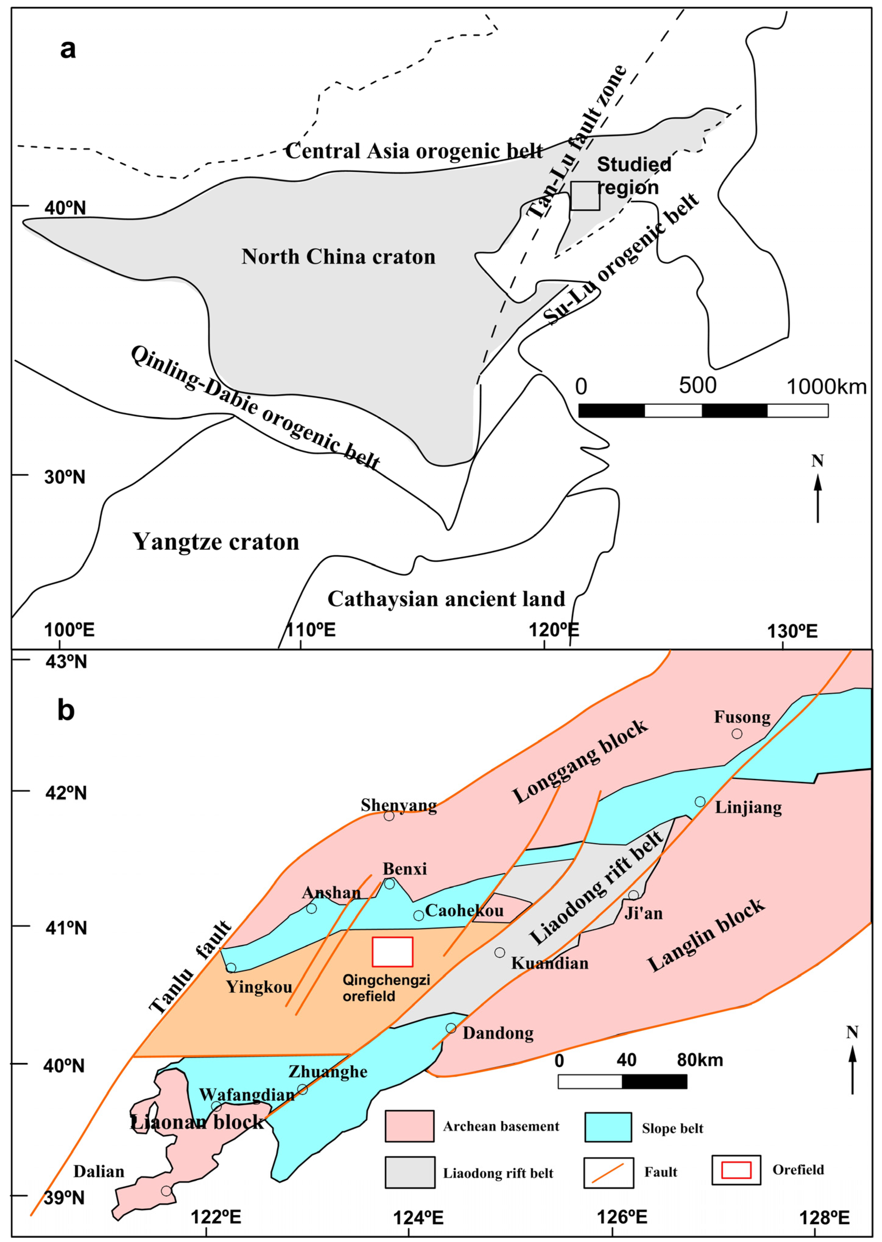
2. Geological Setting

The region has experienced many tectonic activities and magmatic emplacement [18]. The geological structure is complex, dominated by fold structure and characterized by multistage superposition [19] (Figure 2). The Qingchengzi orefield is in the depression zone, along the axis of the Paleoproterozoic Liaodong Rift. The Liaodong Rift is an intercontinental rift developed on the basement of the Archean Craton in North China. After a long evolution, it has deposited thick Liaohe Group strata. The lower part is the volcaniclastic rock formation of the Langzishan Formation and the Lieryu Formation. The middle part is the carbonate formation of the Dashiqiao Formation. The upper part is the terrigenous clastic rock formation of the Gaixian Formation.

A set of strata of the Gaojiayu Formation, Dashiqiao Formation, and Gaixian Formation, belonging to the Proterozoic Liaohe Group metamorphic rock series, is exposed (Figure 2). The ore-bearing rocks are mainly biotite granulite, silicified marble, and an interlayer fracture zone at the contact point with the mica schist of the Gaixian Formation in the third member, and four and five layers of the Dashiqiao Formation. The interlayer fracture zone has been completely or mostly replaced by strong silicified rocks. The structure in the mining area is typical of the northwest Jianshanzi Fault. The fault zone starts from Yangjialing in the south, extends northwestward to the Baiyun gold mine, through the north of Xiaotongjiapuzi and Taoyuan, and extends intermittently for 15 km. It is the main gold ore-controlling structural belt in the mining area.

3. Materials and Methods

3.1. Materials

Because the scale of the target gold ore body and associated quartz vein or pyrite in the study area is small compared with the surrounding rock, it is difficult to detect the ore body directly. Therefore, the ore-bearing strata and ore-controlling structures are the main targets of TEM exploration. These geological targets mainly include Gaixian Formation schist, Dashiqiao Formation marble, and fault and fracture zones. These strata and structures are closely related to the mineralization of the region [19,20,21,22,23]. The existing physical property data show that there are obvious resistivity differences between the main target geological bodies. Using the transient electromagnetic method (TEM) is effective for these physical property conditions [24].

TEM lines were performed in the Qingchengzi orefield. The TEM survey line, named P2, is one profile to explore the geological structure of the striped area of Taoyuan–Linjiasandaogou–Yangshu (see Figure 2). The length of P2 is nearly 10 km, with survey points ranging from 0 to 386. The survey point interval is 50 m. Fixed-loop configurations were used in the field data collection. Ten 400 by 900 m transmitting loops were used for measuring points at different positions, powered with 20 A, using the Crone transmitter. The base frequency was 2.5 Hz (time base was 100 ms). The ramp time was 1000 μs, and a quartz clock synchronous mode was chosen. Time channels ranged from 54 μs to 87.655 ms. In addition, the anti-interference measures of multiple stack times and multiple repeated observation times were adopted in data acquisition, which can obtain better original data and improve the reliability of late time channels.

Figure 3 shows the corresponding relationship between a single transmitting loop and its measuring points during field measurement. After the measurement of a station in the loop was completed, the next transmitting loop was arranged, and the measuring points of the continuation part of the measuring line were implemented.

The transmitting system was the PEM (Pulse Electromagnetic) system (CDR2, Crone Company, Mississauga, ON, Canada), consisting of a 7 kW gasoline generator, a rectifier, a transmitter, and the loop laid on the surface of the earth. The maximum power of the transmitter is 4.8 kW, and its maximum voltage and current are 230 V and 30 A, respectively. The synchronization mode between transmitter and receiver was a quartz clock. The receiver was a Crone Digital PEM. The SQUID magnetometer (GXCD-2, Institute of Geophysical and Geochemical Exploration, Chinese Academy of Geological Sciences, Langfang, Hebei, China) and PEM coil were used as the sensors. The SQUID magnetometer was cooled with liquid nitrogen at 77 K in a Dewar, and the current volume of a broadband non-magnetic Dewar is 2.5 L.

The current version of the SQUID magnetometer performs with noise (60 fT/), slew rate (0.8 mT/S), dynamic range (100 dB), sensitivity (6.25 mV/nT), and bandwidth (DC-20 kHz) [25,26,27,28,29,30,31,32], which effectively accompanies the Canadian Crone PEM system.

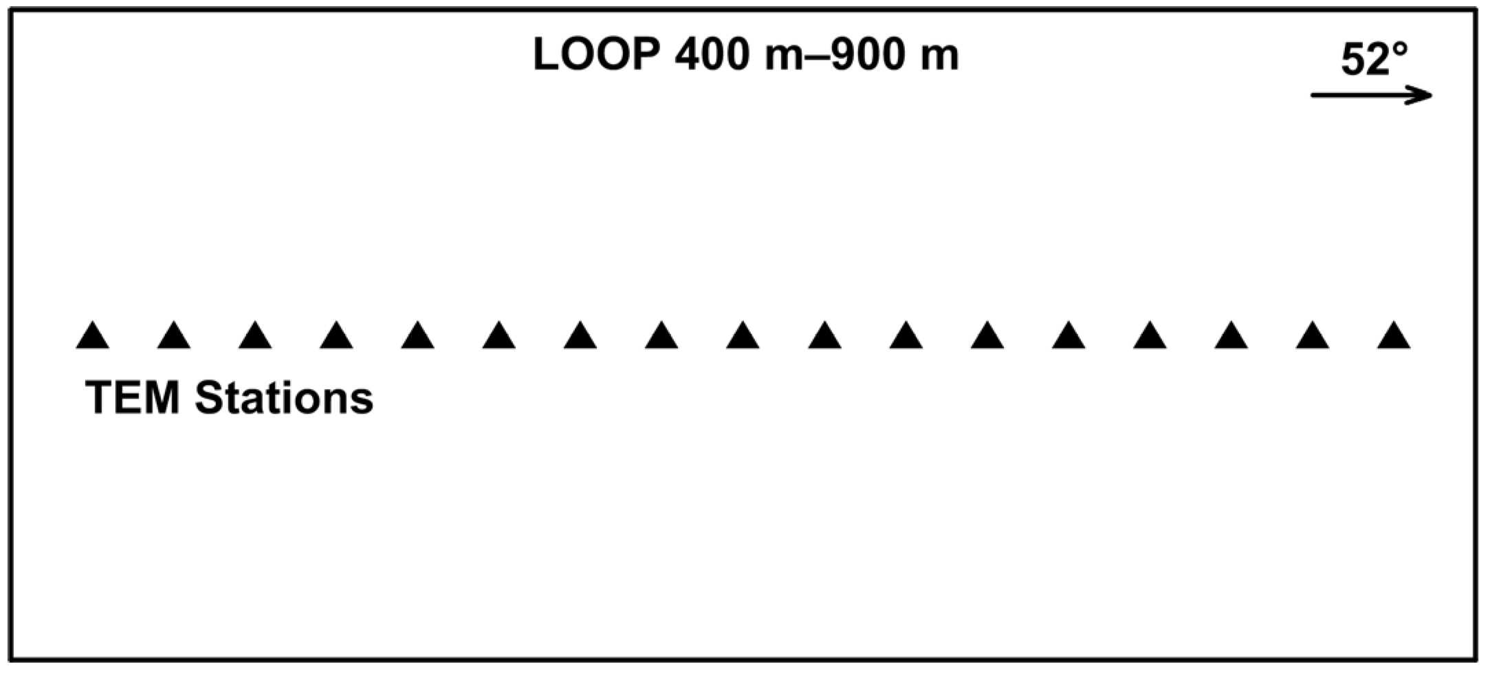
3.2. Methods

The TEM method is an important geophysical prospecting method for metal mineral exploration. This method usually generates a stable primary field with a current in the ground transmitting loop, and then uses current shutdown to stimulate the underground medium and target to generate a secondary field that decays with time. The conductivity of the underground medium can be obtained by observing the attenuation of the secondary field with a TEM sensor. The conventional TEM uses an induction coil to measure the induced electromotive force, or the derivative of the induced magnetic field. In shallow detection, the induced magnetic field changes, and the measurement of its derivative is effective. However, for deep targets, when the change in magnetic field gradient is less than noise, the measurement of the magnetic field derivative cannot meet the requirements [33,34]. A superconductive quantum interference device (SQUID) magnetometer can directly measure the induced magnetic field and has a good signal-to-noise ratio at low frequency [35,36,37]. As the induced magnetic field decays more slowly than its derivative, SQUID can measure the effective observation time longer than the conventional induction coil, and obtain more reliable late data. High signal-to-noise ratio at low frequency can ensure the resolution of deep targets. Previous studies have shown that the TEM based on a SQUID magnetometer has significant advantages in deep exploration [35,36]. Therefore, the SQUID TEM was selected to detect the deep geological structure. In this paper, SQUID TEM was compared with conventional coil TEM. The research results give the electrical characteristics of the deep geological structure in the Taoyuan–Xiaotongjiapuzi–Linjiasandaogou area. This study can also provide a basis for the study of stratigraphic and tectonic evolution.

The TEM method uses a transmission loop to send a primary magnetic field underground, and a current pulse square wave is supplied by the transmission loop. When the trailing edge of the square wave falls, a primary magnetic field that can propagate to the underground is generated. Under the excitation of the primary magnetic field, the geological body will produce eddy current.

For geological prospecting, the attenuation process of the eddy current field is measured by instruments on the surface, and the strength change in the secondary field is used to judge the distribution of underground resistivity. The spectrum information of square wave ramp time is rich, so the spectrum of the secondary field induced by the geological body is also rich [38,39]. In the TEM, the high-frequency component is dominant in the early stage data, reflecting shallow information. Low-frequency components are dominant in late-stage data, reflecting deep geological information.

The data processing of SQUID TEM is based on magnetic field components, and its response simulation is realized by digital filtering technology. For the sake of verifying its accuracy, the analytical solution of the transient electromagnetic dB/dt response is compared with the discrete derivative of the magnetic field response with respect to time. For uniform half-space, the analytical expression of the transient electromagnetic dB/dt response can be written as follows:

$$\frac{d{B}_z}{dt}=\frac{3I_0\rho }{a^3}\left[\varphi \left(u\right)-\sqrt{\frac{2}{\pi }}u\left(1+\frac{u^2}{3}\right)e^{-u^2/2}\right]$$

where ρ is the resistivity of the half-space, a is the radius of the transmitting loop, I₀ is the transmitting current, μ₀ = 4π × 10⁻⁷ is the permeability in vacuum, $u=\sqrt{\frac{{\mu }_0}{2\rho t}}a$, t is the sampling time, and $\varphi \left(u\right)=\sqrt{\frac{2}{\pi }}{\displaystyle {\int }_0^u{e}^{-t^2/2}dt}$ is the probability integral.

A uniform half-space and H-type model were used for calculation and analysis, respectively, where the resistivity of uniform half-space was 100 Ω·m. Parameters of the H-type model are shown in

Table 1. Parameters of H-type model.

Parameters	Layer 1	Layer 2	Layer 3
H (m)	300	100	-
ρ (Ω·m)	100	10	100

. The transmitting loop has an equivalent radius of 200 m, the transmitting current is 1A, and the receiver is located at the center of the loop. The calculation results of the uniform half-space model and H-type model are shown in Figure 4a,b, respectively. It can be observed from the figure that the responses derived from the derivative of the SQUID TEM magnetic field are in good agreement with dB/dt, and the mean square relative errors of the half-space model and H-type model are 0.26% and 1.52%, respectively, which meet the accuracy requirements of the SQUID TEM simulation algorithm.

4. Results

The field data acquisition included both IGGE (Institute of Geophysical and Geochemical Exploration) SQUID and PEM coil receiving sensors. Figure 5 shows the measured TEM decay curves of the two sensors, giving a comparison of the data from the two sensors at different positions on the survey line. Figure 5a shows the original decay curve of the SQUID data, and Figure 5b shows the original decay curve of the coil data.

It can be observed from the figure that the measured B-field data of the SQUID span four orders of magnitude, from early to late time channels, while the dB/dt data span six orders of magnitude, and the attenuation of the B-field data is significantly slower than that of the dB/dt data. The amplitude of the B-field at late channels is approximately 100 pt, while the response amplitude of time channels exceeding 10 ms in the dB/dt data is generally lower than 10 nV. Therefore, the number of reliable data of SQUID that can be used in the inversion is more than the dB/dt data. The time channel of the SQUID data available for inversion generally exceeds 50 ms, while most dB/dt data do not exceed 30 ms. Therefore, the SQUID data contain more late signals. The comparison results show that the attenuation of the B-field data measured by SQUID is slower than that of the dB/dt data, and has a stronger response value, higher signal-to-noise ratio, and more available channels in the late time data.

Figure 6 shows the field SQUID TEM plot curves of points from 90 to 386. In general, the profile curve is smooth and the data quality is good. It can be observed from the profile curve that the transient response value of section 90–250 is generally high, reflecting the good conductivity of the formation in this section.

The 90–386 point segment was selected for inversion, where the data containing the polarization effect were not involved in the inversion.

A pseudo-2D inversion method was adopted for data processing and interpretation. The apparent resistivity was calculated according to the full-field resistivity calculation method of transient magnetic fields, and then the apparent depth was calculated according to the eddy current diffusion velocity of smoke ring theory. The transverse same depth layer is divided into several thick plate-like conductive media with finite lengths using the finite-length thick plate program for forward fitting, and the depth resistivity correction to obtain the final depth resistivity geoelectric section, and determine the distribution of underground electrical structures. This inversion method takes into account the lateral variation in adjacent measuring stations, which makes the calculation results more reasonable [40]. In the inversion, the start model is the result of full-field apparent resistivity, and the constraints are mainly applied to the conductivity difference between adjacent thick plates. The vertical cell numbers is 36, corresponding to the time channels, and the transverse cells are 50 m, corresponding to the survey point intervals. The comparison between the measured curves and the inversion fitting curves is shown in Figure 6. Although the early time channel fitting of 190–250 measuring points is not ideal, the inversion curves on other measuring points fit well with the measured curves, and the overall fitting error is 6.266%, indicating the rationality and reliability of the inversion results.

Figure 7 is a comparison diagram of the SQUID data inversion results and induction coil data inversion results on the same TEM line. Figure 7a is the inversion apparent resistivity section of the induction coil, and Figure 7b is the inversion resistivity section of SQUID. In the comparison figure, blue indicates low resistance and red indicates high resistance. The two results (Figure 7) reflect the same electrical structure. In the inversion results, the overlying high-resistivity stratum is the reflection of the schist of the Gaixian Formation, which is mainly caused by sillimanite biotite schist, biotite schist, and biotite granulite. The middle blue low-resistivity layer is the overall reflection of the third member of the Dashiqiao Formation. Its low-resistivity characteristics are mainly caused by graphite bearing marble and a fault fracture zone. The lower stratum is Dashiqiao section 2, which is dolomitic marble with high resistivity. It can be observed from the figure that the horizontal distribution of the stratum is uneven, and the interface fluctuates greatly, which mainly reflects the fold shape of the stratum in the compression environment.

It can also be observed from Figure 7 that the inversion results of the two types of data are different in some places. First, the inversion depth of the SQUID data is greater than that of the induction coil data. In the conductive area of sections 160–250, the average inversion depth of the induction coil is approximately 1000 m, which fails to reflect the bottom interface of the conductive area. However, the effective inversion depth of the SQUID inversion results in this section exceeds 2000 m, which clearly reflects the folding state of the bottom interface of graphite-containing marble and the lower dolomite marble stratum, and demonstrates the advantages of the SQUID magnetometer in the conductive area. In sections 90–240, the SQUID inversion results reflect the structural characteristics of the stratigraphic syncline, but it is difficult to draw this conclusion due to the lack of lower stratigraphic information in the induction coil inversion results.

Second, the inversion results of the SQUID and induction coil data show resistivity discontinuities below 156 points. We speculate that this result is due to the fracture in the syncline core under compression, which is more obvious in the SQUID inversion results.

Third, the two inversion results show a low-resistivity area below the 120–140 point section, but the induction coil shows low resistance only at the depth of 200–600 m, and the resistivity value below becomes higher. The SQUID data inversion results show this part of the low-resistivity area extending to a greater depth.

Fourth, there is a conductive layer of graphite-containing marble at the depth of 300–400 m in the shallow part of the 250–340 point section. Both results are shown, and the coil inversion results are more obvious. It is likely that this outcome is mainly due to the shallow part of the high-resistivity area. The derivative of the induced magnetic field observed by the coil is more sensitive than the magnetic field itself [33].

5. Discussion

In the TEM-measured data, there is an inverse sign phenomenon in some measured point data [41,42,43]. The original curve does not decay as gradually as a positive value as the curve in Figure 5, but decays rapidly to a negative value from the middle channel to the late channel. Some curves even decay from a positive value to a negative value, and then become a positive value. The reason for these outcomes may be the induced polarization phenomenon of pyritization under the condition of magnetic polarization, due to fracture and alteration under the measuring point [42]. Previous studies have shown that the existence of gold in this area is positively correlated with pyrite, and the polarization phenomenon in the late stage also reflects the pyritization that may be related to gold mineralization in the deep areas. Therefore, the polarization effect produced by pyritization can be considered to be related to gold mineralization. Therefore, the polarization phenomenon in the late stage of the TEM curve has indicative significance and important research value.

Figure 8a is the original decay curve of SQUID, and Figure 8b is the original attenuation curve of the induction coil at the same point. The polarization phenomena with different negative values are listed in Figure 8a. The negative values occur at different times, and to different degrees. In the induction coil data, this phenomenon is only obvious in the curve of point 62, and the negative value phenomenon in the curves of other measuring points is slightly displayed, but its value is equivalent to the noise level, and is not obvious.

To better understand the difference in the polarization phenomenon between the SQUID data and induced coil data, comparative tests under different launch time base conditions were carried out. To analyze the law of the polarization phenomenon, the SQUID and coil data were compared under different time base conditions. Figure 9 presents the original curve of the two sensors under different launch time base conditions, showing the comparison of the SQUID and coil data. Figure 9a shows the original curve of the SQUID data and Figure 9b shows the original curve of the coil data. The negative part has been taken as positive in the figure and drawn with a dashed line. The figure shows that under different timebase, negative values appear in the SQUID data, while the coil data only display noise at late time channels, and the existence of the polarization phenomenon cannot be observed. In addition, the time channels of negative values in different time bases of the SQUID data are basically the same, and the amplitude of negative values is different. It is speculated that this outcome may be caused by the different charging times of the polarizer, due to different time bases.

6. Conclusions

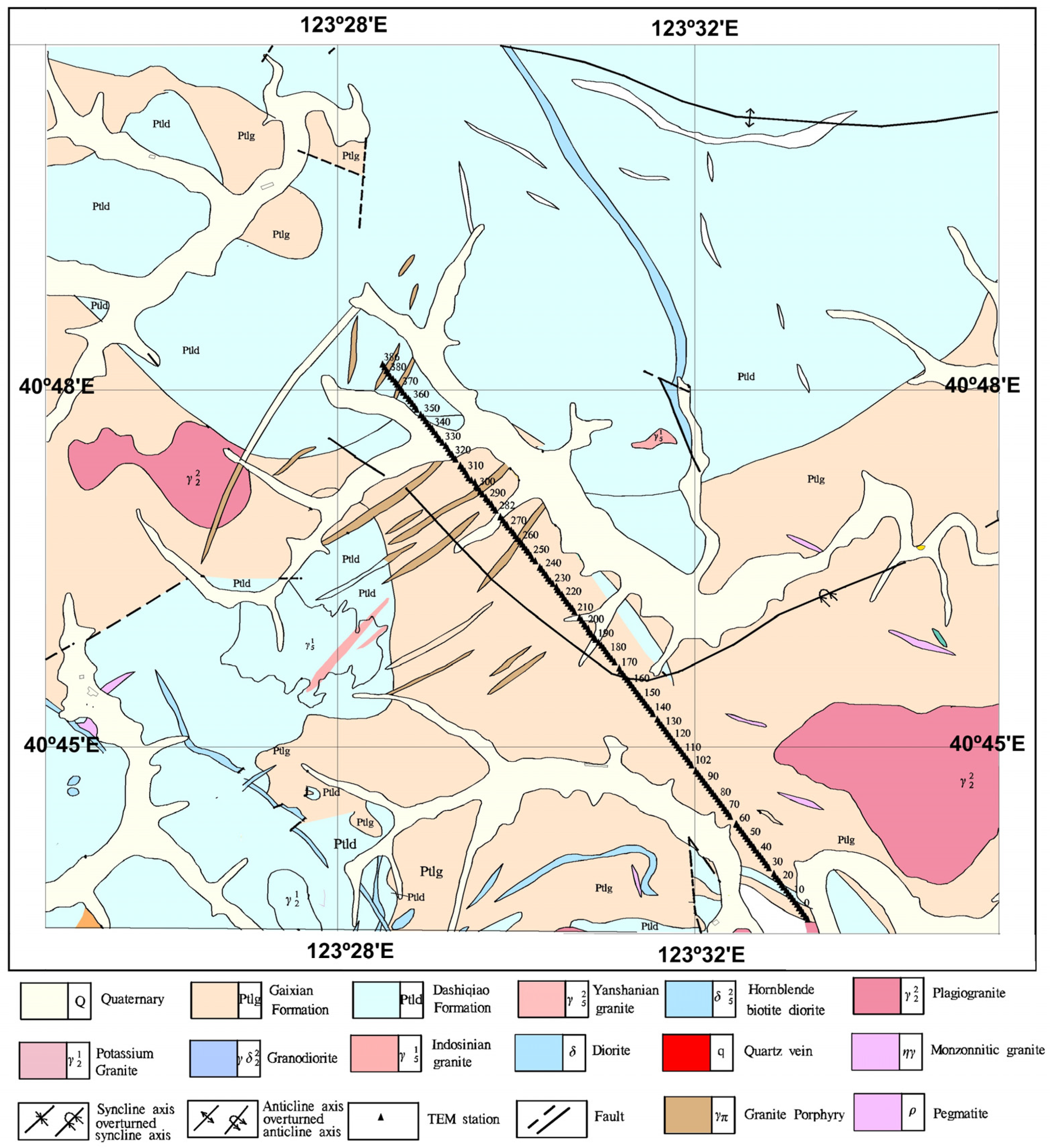
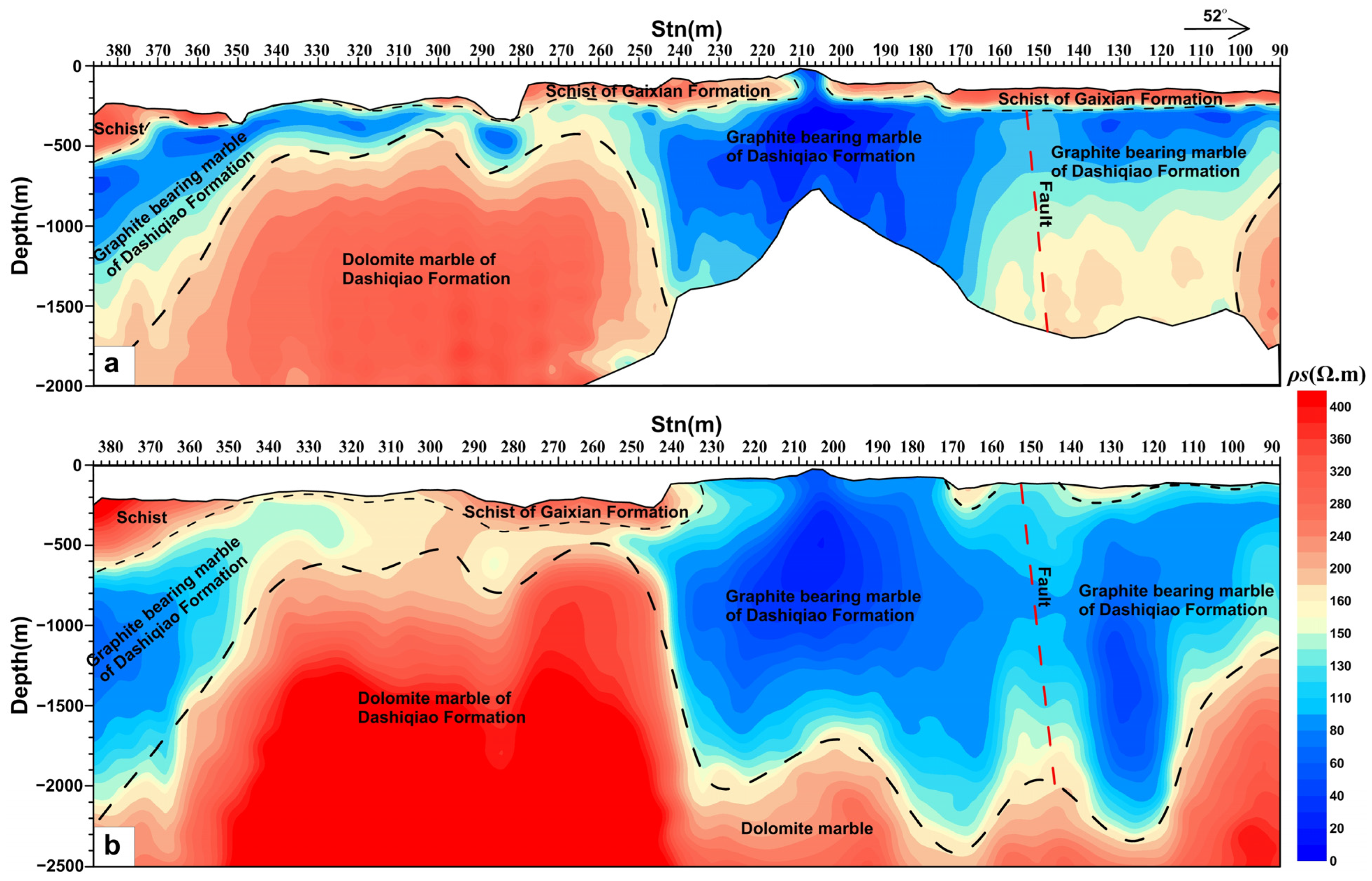
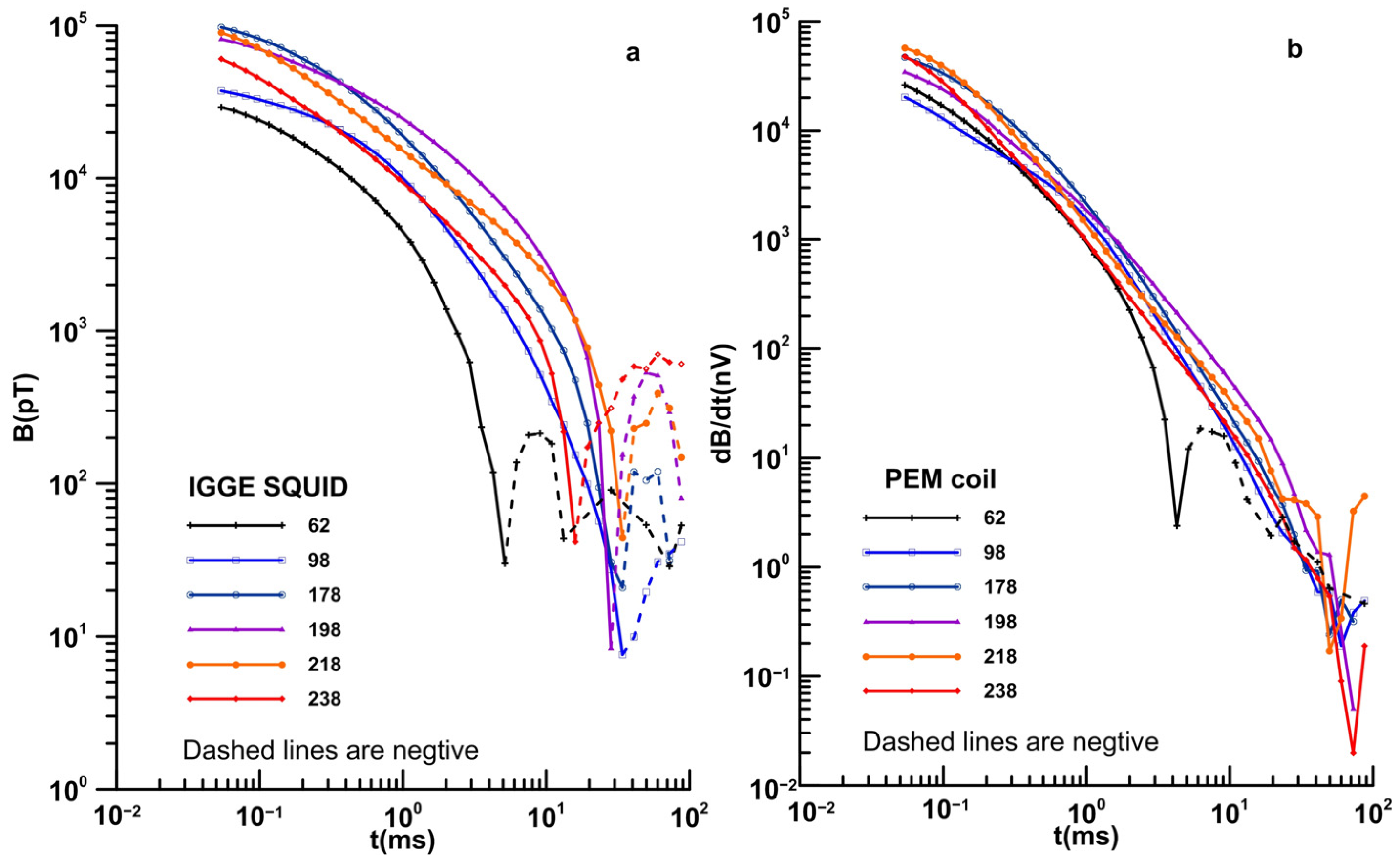
• The stratigraphic structure below the TEM section is generally a syncline structure, and there are secondary crumpled structures at the marble stratigraphic interface of the Dashiqiao Formation, with a depth of about 1500 m in the section 90–230 on the south side of the section, which is characterized by high resistivity. The 90–230 section is a high-conductivity area below 1500 m, which reflects the graphite-bearing marble and fracture zone of the Dashiqiao Formation, and is speculated to be a favorable area for deep gold mineralization. Negative values appear in the SQUID data of some stations, to varying degrees. This polarization phenomenon may be related to deep mineralization.
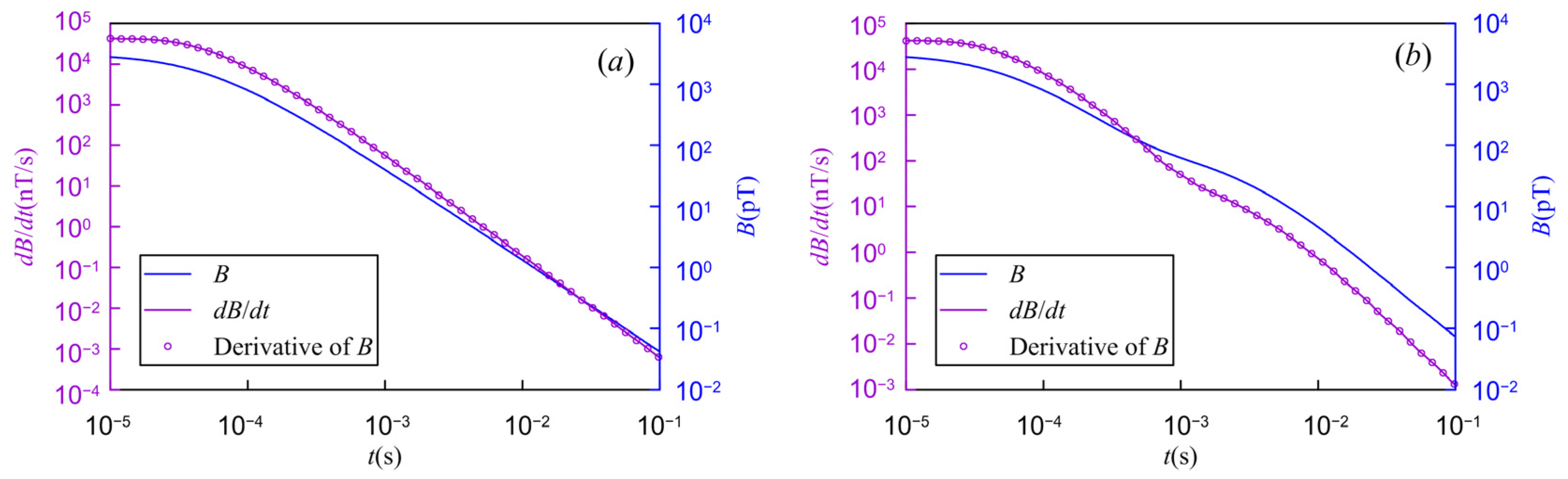
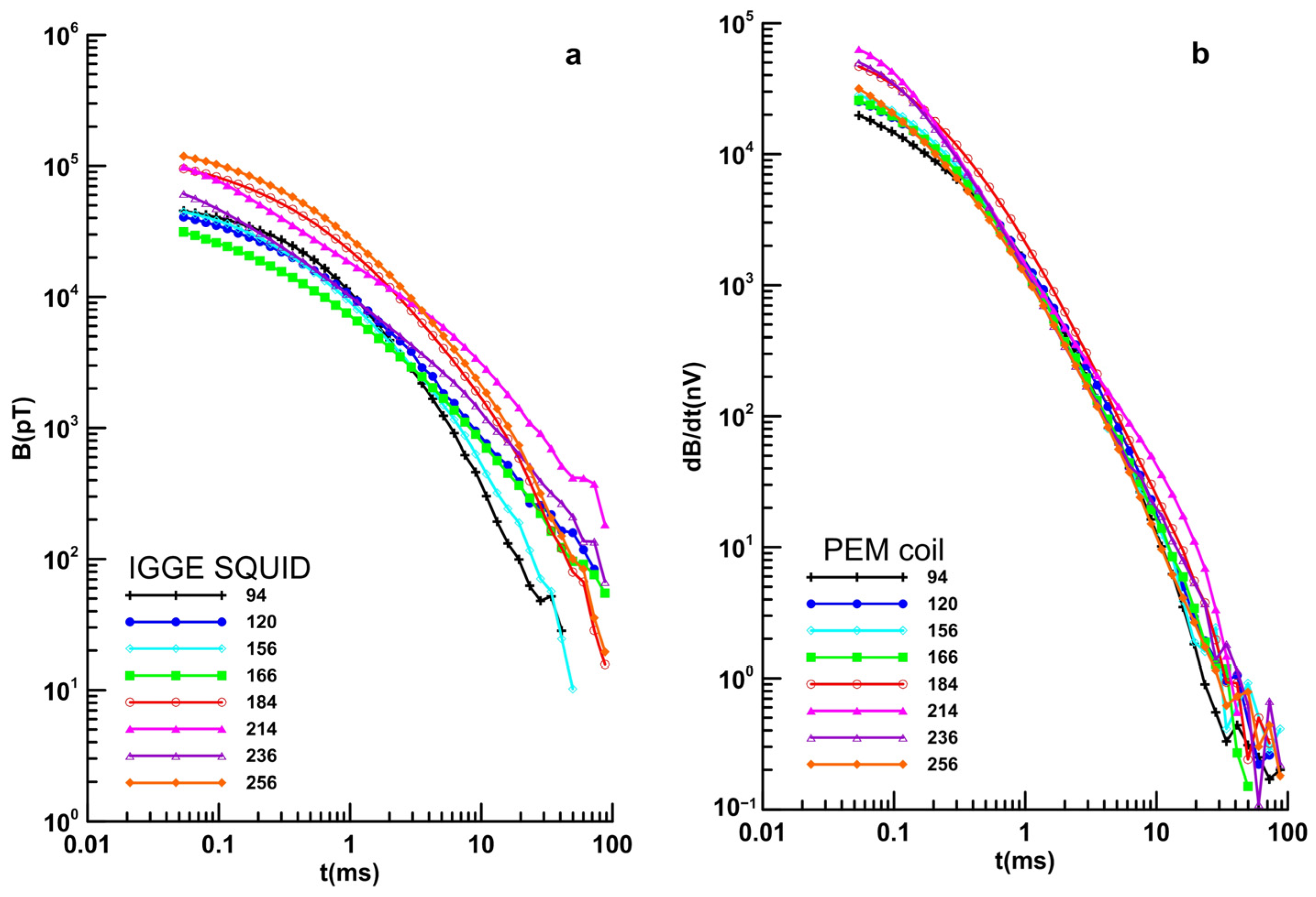
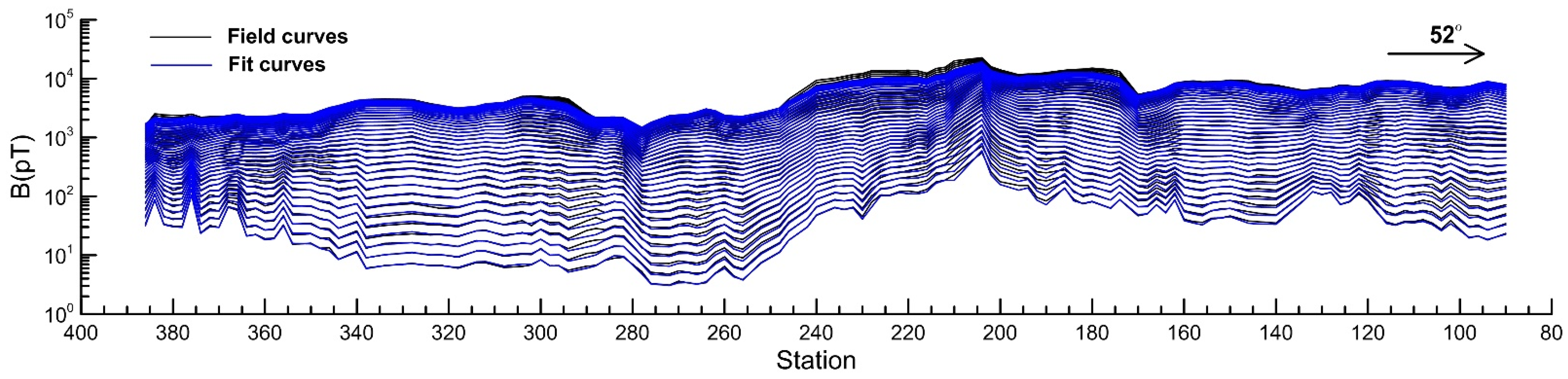
• The deep prospecting test carried out in the Qingchengzi ore concentration area shows that the SQUID TEM system has the advantages of the direct measurement of B-field, a long effective observation time, a high signal-to-noise ratio, and a significant exploration depth, especially in the conductive area. In the shallow detection of the high-resistance region, the dB/dt data are more sensitive to the conductive layer than the B-field data. The dB/dt data inversion results show the conductive layer more clearly than the B-field data in the high-resistivity region.
• Due to the obvious electrical difference in each lithology and stratum in the Qingchengzi ore concentration area, TEM has good application preconditions, and its inversion results can clearly reflect the fold shape of the stratum interface and the developed faults. Applying a large emission magnetic moment, a long time base, and a SQUID sensor has achieved good exploration outcomes.

References

- Di, Q.Y.; Xue, G.Q.; Lei, D.; Zeng, Q.D.; Fu, C.M.; An, Z.G. Summary of technology for a comprehensive geophysical exploration of gold mine in North China. Sci. China Earth Sci. 2021, 64, 1524–1536. [Google Scholar] [CrossRef]
- Zhu, R.X.; Xu, Y.G.; Zhu, G.; Zhang, H.F.; Xia, Q.K.; Zheng, T.Y. Destruction of the North China Craton. Sci. China Earth Sci. 2012, 42, 1135–1159. [Google Scholar] [CrossRef]
- Hou, Z.Q.; Zheng, Y.C.; Geng, Y.S. Metallic refertilization of lishosphere along cratonic edges and its control on Au, Mo and REE ore systems. Miner. Depos. 2015, 34, 641–674. [Google Scholar]
- Zhang, S.H.; Hu, G.H.; Li, J.F.; Xiao, C.H.; Liu, X.C.; Zhang, Q.Q.; Yao, X.F.; Liu, F.X.; Wang, W.; Chen, Z.L.; et al. Ore-Controlling Structures and Metallogenic Favorable Area Prediction in Baiyun-Xiaotongjiabuzi Ore Concentration Area, Eastern Liaoning Province. Earth Sci. 2020, 45, 3885–3899. [Google Scholar]
- Yu, G.; Chen, J.F.; Xue, C.J.; Chen, Y.C.; Chen, F.K.; Du, X.Y. Geochronological framework and Pb, Sr isotope geochemistry of the Qingchengzi Pb–Zn–Ag–Au orefield, Northeastern China. Ore Geol. Rev. 2009, 2009, 367–382. [Google Scholar] [CrossRef]
- Zhao, W.J.; Sha, D.M.; Huan, H.F.; Gao, T. Preliminary structure framework and concealed intrusive rocks in the Qingchengzi ore field in northeast China disclosed by large-scale two-dimensional audio-magnetotelluric sounding. In The Society of Exploration Geophysicist and the Chinese Geophysical Society GEM Xi’an; Society of Exploration Geophysicists: Xi’an, China, 2019; pp. 19–22. [Google Scholar]
- Sun, G.Q.; Wang, S.J.; Sun, H.Y.; Sun, Q.M. Controlled Source Audio Magnetotelluric Survey in the Liaodong Linjiapu Lead-Zinc Mine Prospecting on the Application. Gansu Metall. 2009, 31, 46–47, 106. [Google Scholar]
- Zhang, Z.H.; Liu, F.X. Discussion on the Significance of the Newly Discovered Mineralization Alteration Zone in the Baiyun Gold Deposit, Fengcheng City, Liaoning Province. Acta Geol. Sin. 2015, 89 (Suppl. S1), 251–253. [Google Scholar]
- Liu, Z.Y.; Xu, X.C. Synthetic Information Models and Analyses of Prospecting Perspective of the Qingchengzi Polymetal Metallogenic Mine in Eastern Liaoning Province. J. Jilin Univ. Earth Sci. Ed. 2007, 37, 437–443. [Google Scholar]
- Cheng, S.S.; Peng, L.H.; Sun, D.H.; Sun, D.H.; Wang, Z.H.; Chen, W. The exploration of deep geological structure in the Qingchengzi ore concentration area and its prospecting significance. Geophys. Geochem. Explor. 2021, 45, 859–868. [Google Scholar]
- Floyd, F.S. Remote sensing for mineral exploration. Ore Geol. Rev. 1999, 14, 157–183. [Google Scholar]
- Zhao, P.D.; Chen, Q.M.; Xia, Q.L. Quantitative Prediction for Deep Mineral Exploration. J. China Univ. Geosci. 2008, 19, 309–318. [Google Scholar]
- Xue, G.Q.; Chen, W.Y.; Yan, S. Research study on the short offset time-domain electromagnetic method for deep exploration. J. Appl. Geophys. 2018, 2018, 131–137. [Google Scholar]
- Ahmed, M.E.; Reda, A.Y.E.; Amin, B.P.; Hassan, M.; Milad, S. Integration of ASTER satellite imagery and 3D inversion of aeromagnetic data for deep mineral exploration. Adv. Space Res. 2021, 68, 3641–3662. [Google Scholar]
- Di, Q.Y.; Xue, G.Q.; Zeng, Q.D.; Wang, Z.X.; An, Z.G.; Lei, D. Magnetotelluric exploration of deep-seated gold deposits in the qingchengzi orefield, Eastern Liaoning (China), using a SEP system. Ore Geol. Rev. 2020, 122, 103501. [Google Scholar] [CrossRef]
- Guo, Z.W.; Xue, G.Q.; Liu, J.X.; Wu, X. Electromagnetic methods for mineral exploration in China: A review. Ore Geol. Rev. 2020, 118, 103357. [Google Scholar] [CrossRef]
- He, J.S.; Xue, G.Q. Review of the key techniques on short-offset electromagnetic detection. Chin. J. Geophys. 2018, 60, 1–8. [Google Scholar]
- Zeng, Q.D.; Chen, R.Y.; Yang, J.H.; Sun, G.T.; Yu, B.; Wang, Y.B.; Chen, P.W. The metallogenic characteristics and exploring ore potential of the gold deposits in eastern Liaoning Province. Acta Petrol. Sin. 2019, 35, 1939–1963. [Google Scholar]
- Li, D.D.; Wang, Y.W.; Zhang, Z.C.; Tian, Y.; Zhou, G.C.; Xie, H.J.; Shi, Y. Characteristics of metallotectonics and ore-forming structural plane in Baiyun gold deposit, Liaoning. J. Geomech. 2019, 25, 10–20. [Google Scholar]
- Geng, G.J.; Ma, B.J.; Cong, Y.; Guo, L.L. Discussion on the Thrust Nappe Structure Deformation of Qingchengzi and Gold Ore-controlling, Liaoning Province. Gold Sci. Technol. 2016, 24, 26–31. [Google Scholar]
- Zhang, P.; Li, B.; Li, J.; Chai, P.; Wang, X.J.; Sha, D.M.; Shi, J.M. Re-Os Isotopic Dating and its Geological Implication of Gold Bearing Pyrite from the Baiyun Gold Deposit in Liaodong Rift. Geotecton. Metallog. 2016, 40, 731–738. [Google Scholar]
- Duan, X.X.; Zeng, Q.D.; Yang, J.H.; Liu, J.M.; Wang, Y.B.; Zhou, L.L. Geochronology, geochemistry and Hf isotope of Late Triassic magmatic rocks of Qingchengzi district in Liaodong peninsula, Northeast China. J. Asian Earth Sci. 2014, 91, 107–124. [Google Scholar] [CrossRef]
- Liu, G.P.; Ai, Y.F. Studies on the mineralization age of Baiyun gold deposit in Liaoning. Acta Petrol. Sin. 2000, 16, 627–632. [Google Scholar]
- Wu, J.J.; Zhi, Q.Q.; Deng, X.H.; Wang, X.C.; Yang, Y.; Zhang, J.; Dai, P. Exploration of Deep Geological Structure of Baiyun Gold Deposit in Eastern Liaoning Province with TEM. Earth Sci. 2020, 45, 4027–4037. [Google Scholar]
- Chen, X.D.; Zhao, Y.; Wang, C.J.; Lv, G.Y.; Li, R.C.; Zhang, J. The Development of HTc RF SQUID Magnetometer and Its Field Test in TEM. Acta Geosci. Sin. 2002, 23, 179–182. [Google Scholar]
- Wang, C.J.; Chen, X.D.; Zhao, Y.; Wang, B.Z. Application of 77K SQUID magnetometer in TEM. Chin. J. Geophys. 1999, 42, 161–166. [Google Scholar]
- Wu, J.J.; Chen, X.D.; Yang, Y.; Zhi, Q.Q.; Wang, X.C.; Zhang, J.; Deng, X.H.; Zhao, Y.; Huang, Y. Application of TEM Based on HTS SQUID Magnetometer in deep Geological Structure Exploration in the Baiyun Gold Deposit, NE China. J. Earth Sci. 2021, 32, 1–7. [Google Scholar] [CrossRef]
- Chen, X.D.; Zhao, Y.; Zhang, J.; Lv, G.Y.; Ma, P.; Dai, Y.D. The Applications of HTc SQUID Magnetometer to TEM. Chin. J. Geophys. 2012, 55, 702–708. [Google Scholar]
- Chen, X.D.; Zhao, Y.; Lin, T.L.; Yang, T.; Dai, Y.D. The Applications of HTc SQUID Magnetometer to LOTEM. Geophys. Geochem. Explor. 2012, 36, 65–68. [Google Scholar]
- Chen, X.D.; Zhao, Y.; Zhang, J.; Wu, J.J.; Zhao, J.X.; Xing, T.Z. Influence of Frequency Characteristics of Nonmagnetic Dewar on High Temperature Superconducting Magnetometer. Comput. Tech. Geophys. Geochem. Explor. 2007, 29, 292–303. [Google Scholar]
- Chen, X.D.; Zhao, Y.; Deng, X.H.; Lv, G.Y.; Zhang, J.; Zhao, J.X. The Development of the HTc SQUID Magnetometer and Its Application to TEM. Geophys. Geochem. Explor. 2006, 30, 229–232. [Google Scholar]
- Zhao, Y.; Chen, X.D.; Wang, C.J. The Intelligence Control System of Rf SQUID Magnetometer. Geol. Prospect. 2002, 38, 22–24. [Google Scholar]
- Zhi, Q.Q.; Wu, J.J.; Yang, Y.; Wang, X.C.; Chen, X.D.; Zhao, Y.; Deng, X.H.; Zhang, J. Superiority of BZ-based transient electromagnetic method and verification test in coastal tidal regions. Prog. Geophys. 2020, 35, 379–385. [Google Scholar]
- Le Roux, C.; Macnae, J. SQUID sensors for EM systems. In Exploration in the New Millennium: Proceedings of the Fifth Decennial International Conference on Mineral Exploration; Decennial Mineral Exploration Conferences: Toronto, ON, Canada, 2007; pp. 417–423. [Google Scholar]
- Chwala, A.; Stolz, R.; IJsselsteijn, R.; Bauer, F.; Zakosarenko, V.; Hübner, U.; Georg Meyer, H. “JESSY DEEP”: Jena SQUID Systems for Deep Earth Exploration. In 80th Annual International Meeting, SEG, Expanded Abstracts; Society of Exploration Geophysicists: Denver, CO, USA, 2010; pp. 779–783. [Google Scholar]
- Chwala, A.; Stolz, R.; Schmelz, M.; Zakosarenko; Meyeyr, M.; Georg Meyer, H. SQUID Systems for Geophysical Time Domain Electromagnetics (TEM) at IPHT Jena. IEICE Trans. Electron. 2015, 98, 167–173. [Google Scholar] [CrossRef] [Green Version]
- Arai, E.; Katamama, H.; Hart, J. Application of a new TEM data acquisition system based on a HTS SQUID magnetometer (SQUITEM) to metal exploration in Broken Hill area. ASEG Ext. Abstr. 2007, 1, 1–5. [Google Scholar] [CrossRef]
- Smith, R.; Annan, P. The Use of B-Field Measurements in an Airborne Time-Domain System: Part I. Benefits of B-Field Versus dB/dt data. Explor. Geophys. 1998, 29, 24–29. [Google Scholar] [CrossRef]
- Foley, C.P.; Leslie, K.E.; Binks, R. A history of the CSIRO’s development of high temperature superconducting RF SQUIDs for TEM prospecting. In 18th Geophysical Conference and Exhibition of the ASEG, Extended Abstracts; Taylor & Francis: Melbourne, Australia, 2006; pp. 1–5. [Google Scholar]
- Zhang, J.; Lü, G.Y.; Guo, B.L.; Chen, X.D.; Wu, J.J.; Wang, X.C. The High Temperature Superconductivity TEM Transient Magnetic Field Pseudo-2D Inversion and Its Application Effect. Geophys. Geochem. Explor. 2010, 34, 205–208. [Google Scholar]
- Yin, C.C.; Miao, J.J.; Liu, Y.H.; Qiu, C.K.; Cai, J. The effect of induced polarization on time-domain airborne EM diffusion. Chin. J. Geophys. 2016, 59, 4710–4719. [Google Scholar]
- Spies, B.R. Discussion on “Peculiarities of SQUID Magnetometer Application in TEM”. Geophysics 2004, 69, 624–628. [Google Scholar] [CrossRef]
- Panaitov, G.; Bick, M.; Zhang, Y.; Krausem, H.J. Peculiarities of SQUID Magnetometer Application in TEM. Geophysics 2002, 67, 739–745. [Google Scholar] [CrossRef]