Article

Geochemical and Hydrothermal Alteration Patterns of the Abrisham-Rud Porphyry Copper District, Semnan Province, Iran

1
School of Earth Sciences & Engineering, Tomsk Polytechnic University, 634050 Tomsk, Russia
2
Faculty of Mining, Petroleum & Geophysics Engineering, Shahrood University of Technology, Shahrood 3619995161, Iran
*
Author to whom correspondence should be addressed.
Minerals 2022, 12(1), 103; https://doi.org/10.3390/min12010103
Submission received: 15 October 2021 / Revised: 21 December 2021 / Accepted: 27 December 2021 / Published: 16 January 2022

Abstract

:
In this study, the zonality method has been used to separate geochemical anomalies and to calculate erosional levels in the regional scale for porphyry-Cu deposit, Abrisham-Rud (Semnan province, East of Iran). In geochemical maps of multiplicative haloes, the co-existence of both the supra-ore elements and sub-ore elements local maxima implied blind mineralization in the northwest of the study area. Moreover, considering the calculated zonality indices and two previously presented geochemical models, E and NW of the study have been introduced as ZDM and BM, respectively. For comparison, the geological layer has been created by combining rock units, faults, and alterations utilizing the K-nearest neighbor (KNN) algorithm. The rock units and faults have been identified from the geological map; moreover, alterations have been detected by using remote sensing and ASTER images. In the geological layer map related to E of the study area, many parts have been detected as high potential areas; in addition, both geochemical and geological layer maps only confirmed each other at the south of this area and suggested this part as high potential mineralization. Therefore, high potential areas in the geological layer map could be related to the mineralization or not. Due to the incapability of the geological layer in identifying erosional levels, mineralogy investigation could be used to recognize this level; however, because of the high cost, mineralogy is not recommended for application on a regional scale. The findings demonstrated that the zonality method has successfully distinguished geochemical anomalies including BM and ZDM without dependent on alteration and was able to predict erosional levels. Therefore, this method is more powerful than the geological layer.

1. Introduction

The utilization of geochemical methods for ore deposit exploration dates back to 1930. Fersman (1939) carried out the first survey of such an exploration [1]. Since then, further studies on the theory and application of geochemical exploration methods have been carried out, and these techniques have been increasingly modified and improved. Mining geochemistry is a branch of applied geochemistry, which is based on the utilization of geochemical methods that helps increase the ore reserves of known mines by assessing the ore potential of deep horizons. In other words, local and mine scale exploration models for anomaly recognition are created and developed by using mining geochemistry. Recent experiences in the application of mining geochemistry illustrate its efficiency in the discovery of blind and zone-dispersed mineralization (BM and ZDM) within areas of active and abandoned mines. Due to increasing ore reserves and mining income, this trend in geochemical exploration is very important [2]. The recognition of various alteration zones is a qualitative method that cannot help geochemists in separating BM from ZDM at a local scale. In mining geochemistry, the alteration has no basic role in separating anomalies at a local scale [3,4]. Optimal drilling points were determined by using mining geochemistry as a quantitative method without being time consuming and inducing high costs. In the past decades, several models and methods based on geochemistry have been developed for predicting geochemical anomalies as well as the locations of hidden orebodies [2,5,6,7]. Most of these models and methods are focused on the identification of geochemical anomalies reflecting the presence of hidden orebodies and the prediction of horizons of erosional surfaces [8]. In active mines, vertical geochemical zonality is the most important feature of primary halos because of the relation to the direction of the ore-bearing fluid [9,10,11]. Beus and Grigorian (1977) used vertical geochemical zonality to predict hidden mineralization at the mine scale [12]. Grigorian (1985, 1992) presented a zonality model to identify BM from ZDM [5,6]. Since then, the zonality method has been used in many studies [2,3,4,13,14,15,16,17,18,19,20,21]. Solovov (1987) used metallometric methods for the identification of geochemical anomaly (IGA) and the quantitative evaluation of ore reserves [22]. Baranov (1987) introduced a model in which horizons of the erosional surface were computed for geochemical associations [23]. Solovov (1990) introduced different relations to predict hidden orebodies by using metallometric exploration [24]. Liu and Peng (2004) presented a model to predict hidden orebodies by the synthesis of geological, geophysical, and geochemical information based on a dynamic approach [25].
In most mineral exploration methods (e.g., porphyry-Cu), a mineral potential map is obtained by using one layer or a combination of different layers [26,27,28,29,30,31], which includes field geological surveys, geochemical surveys, field geophysical surveys, and remote sensing [32,33,34]. This map consists of shallow to the deep layers, which poses a problem when these layers are not associated with mineralization. Each of these layers has a value for mapping the areas with the potential of mineralization, and a number of these layers are generally surficial and cannot be useful for identifying BM. Hydrothermally altered rocks result from chemical attacks of pre-existing rocks by hydrothermal fluids. The spatial distribution of hydrothermally altered rocks is a key to locating the main outflow zones of hydrothermal systems, which may result in the recognition of mineral deposits [35]. Minerals associated with alteration can be detected by remote sensing. These tasks are achieved by using the analysis of the spectral signatures recorded in the visible-near infrared (VNIR), short wave infrared (SWIR), and thermal infrared (TIR) regions of the electromagnetic spectrum with this spectral signature constituting the key mineral identification criterion [36]. Furthermore, the mineral deposits are spatially and genetically associated with the various types of geological structures including faults or fractures [37]. Faults and fractures, which transport magmatic, meteoric, and metal carrying hydrothermal fluids, subsequently deposit metals [38]. Zarasvandi et al. (2005); Sillitoe (2010); Mirzaie et al. (2015); Habibkhah et al. (2020); and Yumul Jr. et al. (2020) have investigated the importance of the role of faults/fractures in porphyry-Cu [38,39,40,41,42]. The strong advance in remote sensing allows exploiting a variety of sources and methods in the characterization of lineaments [43]. Remote sensing is a valuable technical resource for mineral exploration when it is properly employed [44,45,46,47,48,49,50,51,52,53].
In this study, the results of the zonality method were compared with the geological layer including rock units, faults, and alterations. For this goal, a part of the 1:100,000 scale map of Abrisham-Rud (Semnan province, East of Iran) was examined. This area is a part of the Troud Range in the Khorasan porphyry tract, which few studies on porphyry mineralization have been conducted [54]. Orojnia (2003) studied the lithology and provenance of Eocene volcanic rocks in this area, which suggested identifying the economic potential of Cu [55]. Mars (2014) suggested the potential of hydrothermal alteration in the Torud Range that could be associated with an unidentified porphyry system [56]. Thus, study data are concentrated in the province of Abrisham-Rud, where it has high propects for porphyry copper mineralization.

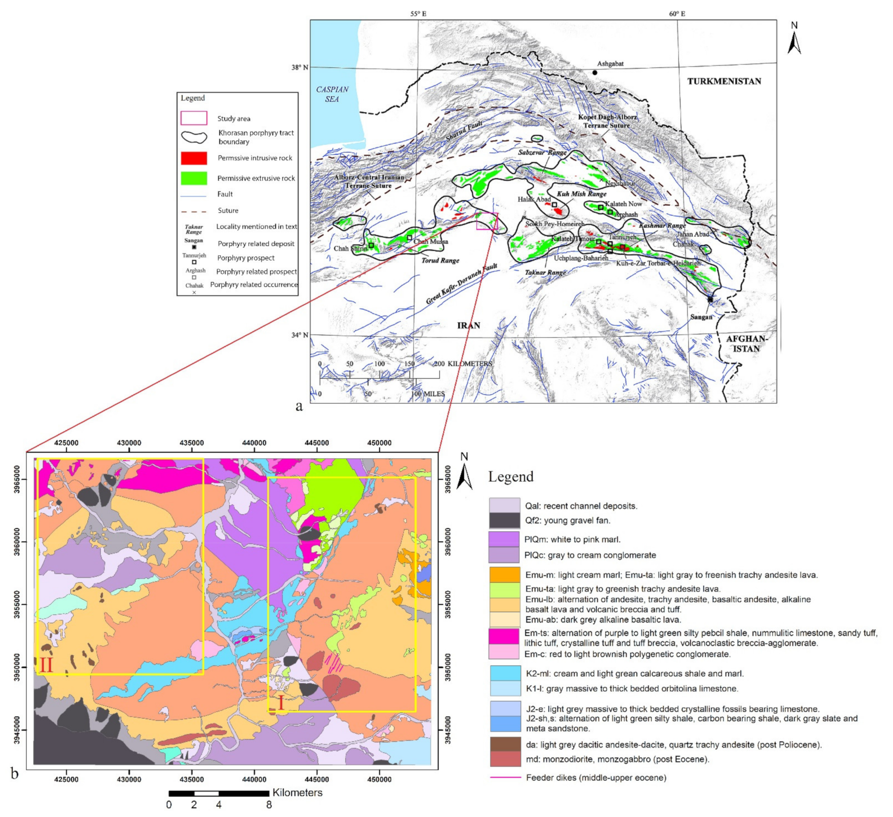
2. Geological Setting of the Study Area

The study area is a part of the 1:100,000 scale map of Abrisham-Rud (Semnan province, East of Iran), which is located in the north of the Central Iran zone [57], and it is a part of Troud Range in Khorasan porphyry tract (Figure 1a). Khorasan porphyry tracts are delimited by permissive units of island arc setting of Late Cretaceous to Early Miocene age [58]. This tract includes four main ranges: Taknar-Kashmar, Kuh Mish, Sabzevar, and Torud [54]. Igneous units of this tract are shown in Figure 1a, along with the location of known porphyry-related mineral occurrences and other geologic features mentioned in this section. In the Torud Range (west of Khorasan porphyry tract), middle Eocene volcano-sedimentary rocks are overlain by Eocene–Oligocene calc-alkaline and alkaline volcanic rocks, which are interlayered with shallow marine, lacustrine, and subaerial sedimentary successions. These successions are intruded by basic tholeiitic dikes and calc-alkaline quartz monzodioritic to granodioritic stocks [59,60]. The aluminum content of hornblendes indicates shallow emplacement depths [61]. In this range, Chah Shirin and Chah Mussa have been introduced as porphyry/porphyry-related deposits [58].
The study area has a dry climate, mountainous topography, and poor vegetation cover. The oldest geological units are metamorphic rocks for which its bedrock was metamorphosed in the Late Triassic. The latest units are associated with a quaternary that consists of gravel fan, terrace, clay and salt deposits, and channel deposits (Figure 1b). Most volcanic activity occurred in semi-arid settings in the form of lava. The middle-upper Eocene rock units are the most extended in the study area and mostly include volcanic breccia-agglomerates and tuffs, intermediate lavas, basic and acidic rocks, and pyroclastic-sedimentary rocks. These units have outcrops and are sometimes dispersed or indistinguishable, and there are many faults in them. The volcanic breccia–agglomerate units that sometimes had intermediate lavas observed in red-brown and sometimes had dusty colors (argillic alteration), as well as the presence of green minerals (chlorite, epidote) in the volcanic fragments of this breccia, indicate lava explosive eruption in a semi-arid and shallow setting with the effect of water on alterations [55].

3. Material

3.1. Geological Data

The 1:100,000 scale map of Abrisham-Rud was purchased from the Geological Survey of Iran (GSI). As shown in Figure 1b, a part of this geological map was selected.

3.2. Geochemical Data

The geochemical database of the 1:100,000 scale map of Abrisham-Rud was also purchased from GSI. The 364 samples have been surveyed in a systematic network with intervals of 1400 × 1400 m2 (Figure 2), and these soil samples have been analyzed using the ICP-MS method. The concentrations of Cu, Mo, Pb, and Zn were considered for this study.

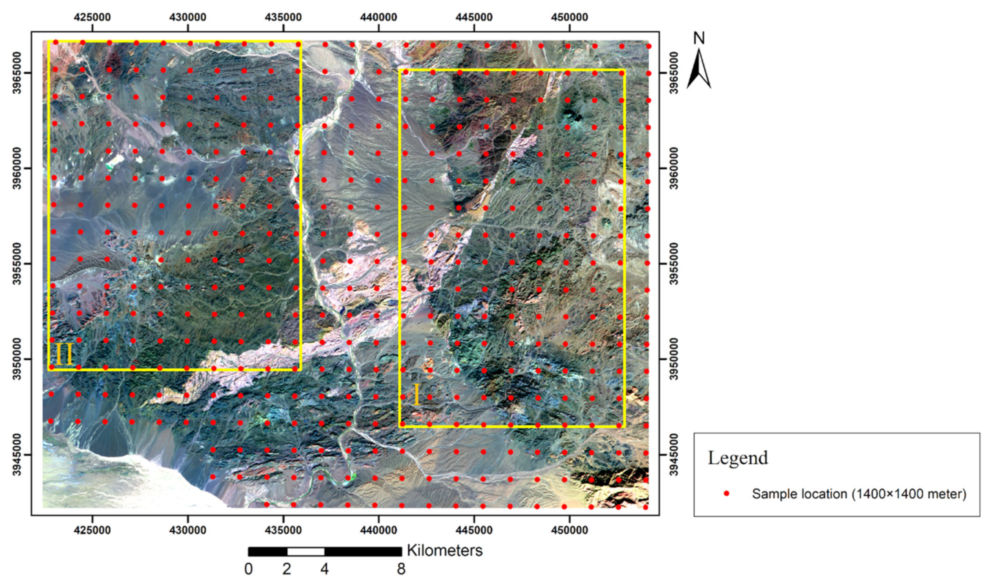
3.3. Remote Sensing Data

In this study, Sentinel-2 MSI-Level 1C and ASTER-Level 1T images were downloaded from the USGS Earth Explorer website (earthexplorer.usgs.gov, accessed on 22 December 2021; Sentinel 2 File: T40SDE_20181118T07015, 20181118-Date of Acquisition (YYYYMMDD); Aster File: AST_L1T_00303282005071248_20150508204820_5306, 03282005-Date of Ac-quisition (MMDDYYYY), 20150508-Date of Processing (YYYYMMDD)).

3.3.1. Sentinel-2 MSI Data

The Sentinel-2 multi-spectral instrument (MSI) satellite carried a high-resolution multispectral imager with 13 bands spanning VNIR through SWIR regions. Sentinel-2 MSI includes 4 spectral bands (bands 2, 3, 4 and 8) at 10 m, 6 bands (bands 5, 6, 7, 8a, 11 and 12) at 20 m, and 3 bands (bands 1, 9, and 10) at 60 m. Sentinel-2 MSI measures reflected radiation in ten bands between 0.433 and 0.955 µm (VNIR) and three bands between 1.36 and 2.28 µm (SWIR) [63,64,65]. In this study, a Sentinel-2 MSI-Level 1C image was used, which is produced from the Sentinel-2 MSI-Level 1B product by radiometric and geometric corrections.

3.3.2. ASTER Data

Advanced Spaceborne Thermal Emission and Reflection Radiometer (ASTER) sensors are one of the multi-spectral sensors that have been installed on the Terra satellite. ASTER measures reflected radiation in three bands between 0.52 and 0.86 µm (VNIR) and in six bands between 1.60 and 2.43 µm (SWIR) and five bands of emitted radiation in the 8.125 µm to 11.65 µm (TIR) region with 15 m, 30 m, and 90 m resolution, respectively [66,67,68]. In this study, an ASTER-Level 1T image was utilized. ASTER-Level 1T data contain calibrated at-sensor radiance, which corresponds with ASTER-Level 1B that has been geometrically corrected and rotated to the north up UTM projection.

3.3.3. Data Preparation

Atmospheric correction was used to minimize influences of atmospheric factors in multispectral data. The Internal Average Relative Reflection (IARR) method was applied to Sentinel-2 and ASTER data. The IARR technique for mineral mapping requires no prior knowledge of geological features [69]. The average radiance for each band of the image was calculated; therefore, an average spectrum was created, and this average spectrum was divided into actual radiance for each band of each pixel to create an image of apparent reflectance. It has been suggested as the best method for arid areas with no vegetation cover [70].

4. Methodology

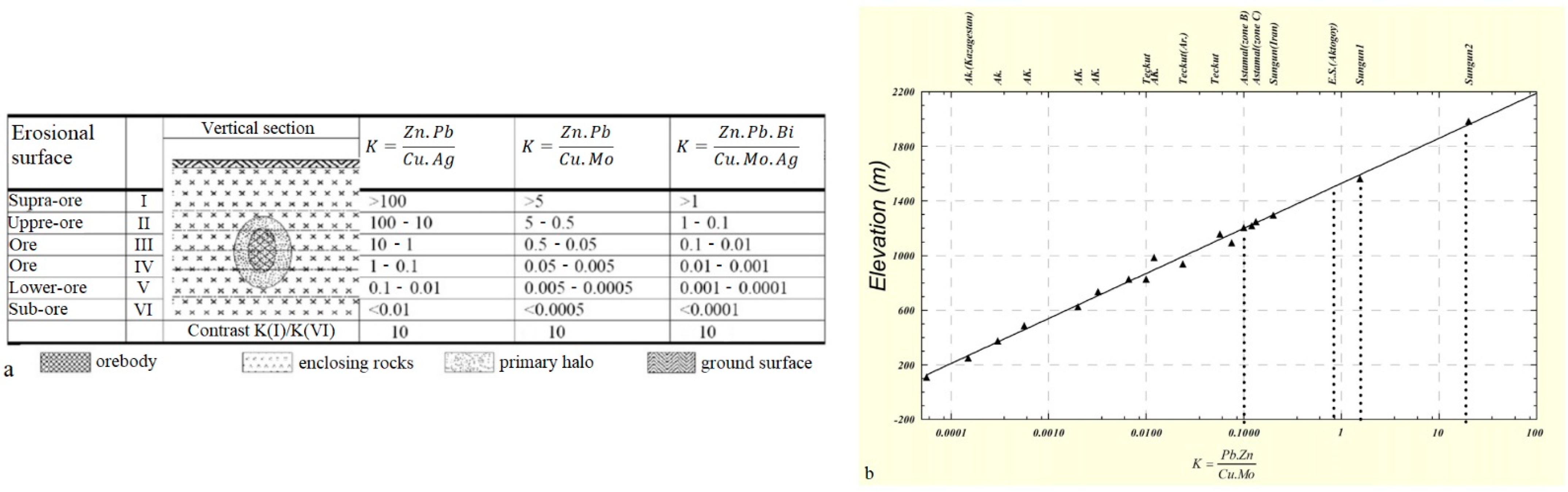
4.1. Zonality Method

A zonation of a geochemical halo has a spatial nature and vectorial context that can be defined by the three parameters of dimension (space), direction, and element concentration [4]. Recognition of zonality of geochemical halos associated with BM can be achieved using four cases of complementary analyses [2]: (1) analysis of element associations representing supra-ore and sub-ore halos of mineral deposits; (2) analysis of a single component, implying false anomaly; (3) analysis of mean values of indicator elements outside significant geochemical anomalies to eliminate background noise in data analysis; and (4) mapping of multiplicative geochemical anomalies.
One of the most important indices in porphyry-Cu deposits is the ratio of Pb and Zn to Cu and Mo, which is often defined as a zonality index [2,12,71]. This index represents different exhumation levels of mineral deposits [6]. Input variables can be subdivided into the following: supra-ore, upper-ore, ore, lower-ore, and sub-ore [24]. Ziaii et al. (2012) and Ziaii et al. (2009) showed that these groups provide the necessary information to separate BM from ZDM in porphyry-Cu mineralization [2,3].

4.1.1. Anomaly Separation

For mapping the multiplicative index of supra-ore (Pb × Zn) and sub-ore (Cu × Mo) elements and calculating the zonality index, the threshold value is calculated by using Equation (1) for each element:
CA = Cx εt,
where CA is the anomaly value, and Cx = Co is the geometric mean of the elements contained within the background area, which is calculated by using Equation (2):
C x ˜ = ant log ( 1 N i = 1 N log C i ) ,
ε = ant log ( i = 1 N ( log C i log C x ˜ ) 2 N 1 ) ,
Where Ci is the element concentration of samples, N is the number of samples, and ε is generally called a standard factor, which is calculated from Equation (3). Due to the above consideration as to the selection of the value of t, the lowest anomalous content, when trying to detect weak anomalies determined from one sampling point, in geochemical prospecting it is taken equal to CAl ≥ Coε3. This relationship corresponds to a “three standard deviations” criterion extensively used in many engineering disciplines to determine quantities falling outside the probable values of a random anomaly distributed quantity. Thus, weak anomalies formed by a sequence of adjacent sampling points with increased pathfinder elements below CAl can be detected, and it is conventional to lower the threshold value according to the criterion CAm≥ Coε3/√m, where m = 2, 3, 4…9 is the number points that may be joined, which can show a common anomaly in the geochemical map [22].

4.1.2. Erosional Surface

In order to predict the erosional level, Solovov (1987) suggested using areal productivity, and Beus and Grigorian (1977) suggested using the coefficient of mineralization to eliminate the syngenetic parameters of the halos, which increase anomaly detection [12,22]. It should be noted that both the areal productivity and mineralization coefficients are used to calculate the vertical geochemical zonality index.
In the systematic sampling network, linear productivity is calculated according to Equation (4):
M = Δ x ( x = 1 n C x nC ) ,
where M is the linear productivity, Δx is the distance between the samples in each profile, Cx is the values greater than the anomaly concentration, and n is the number of anomal samples. If the values of Mi are preliminarily estimated in each of m profiles across the anomaly, P is determined according to Equation (5) [22]:
P = 2 l ( i = 1 m M i ) ,
where 2l is the distance between profiles. Therefore, the zonality index introduced by Solovov (1987) is calculated for zones I and II by using Equation (6) [22].
K S = P ( Pb ) × P ( Zn ) P ( Cu ) × P ( Mo ) ,
The zonality index introduced by Beus and Grigorian (1977) is calculated for each zone by using Equation (7) [12]:
K G = η ( α ) Pb × CA ¯ Pb × η ( α ) Zn × CA ¯ Zn η ( α ) Cu × CA ¯ Cu × η ( α ) Mo × CA ¯ Mo ,
where CA is the arithmetic mean of element contents, and η(α) is the coefficient of mineralization calculated for each element by using Equation (8):
η ( α ) = η A ( α ) ore η A ( α ) ,
where η(α)ore is the number of anomalous samples, and ηA(α) is the total number of samples in each zone [12].

4.2. Remote Sensing

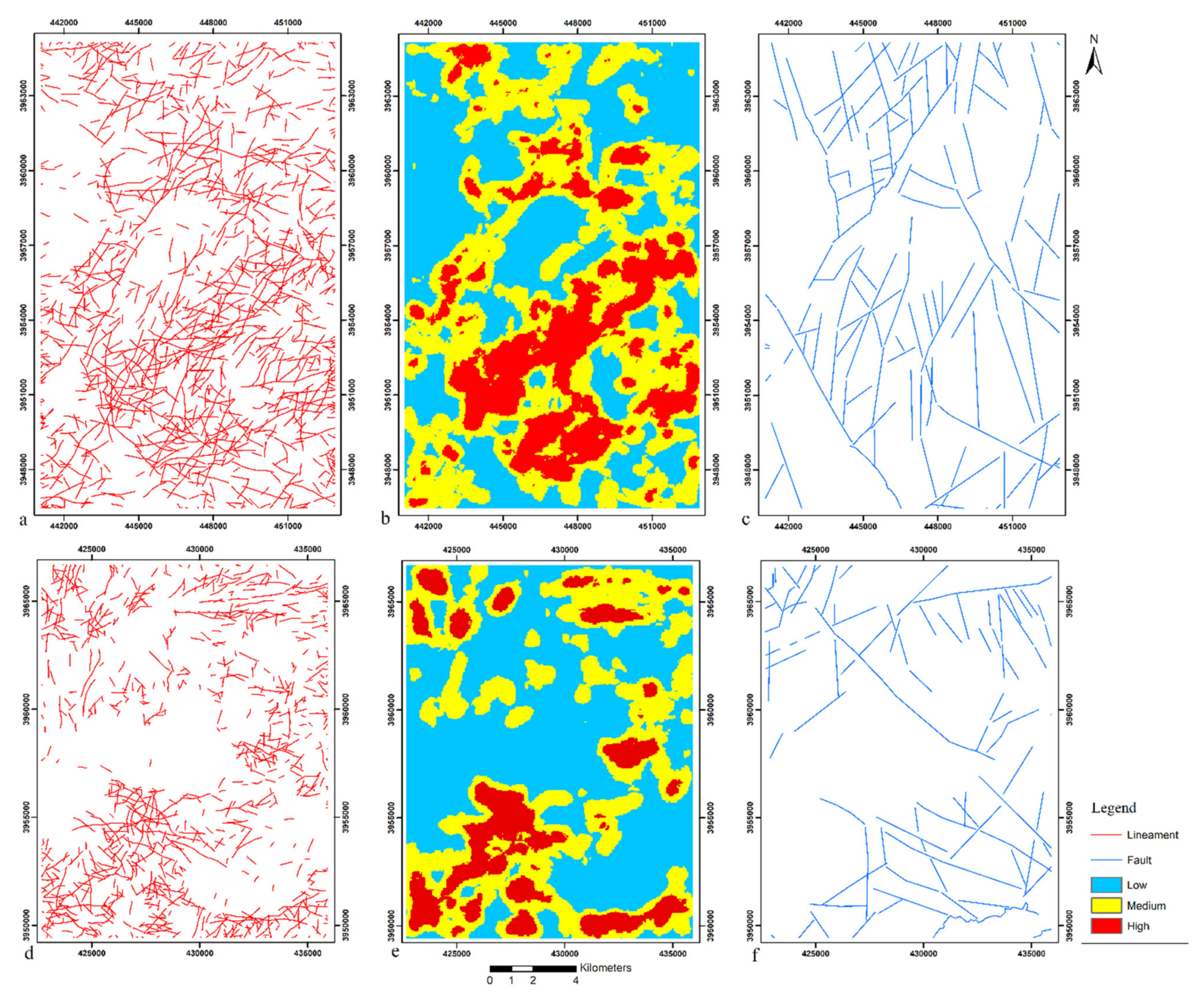
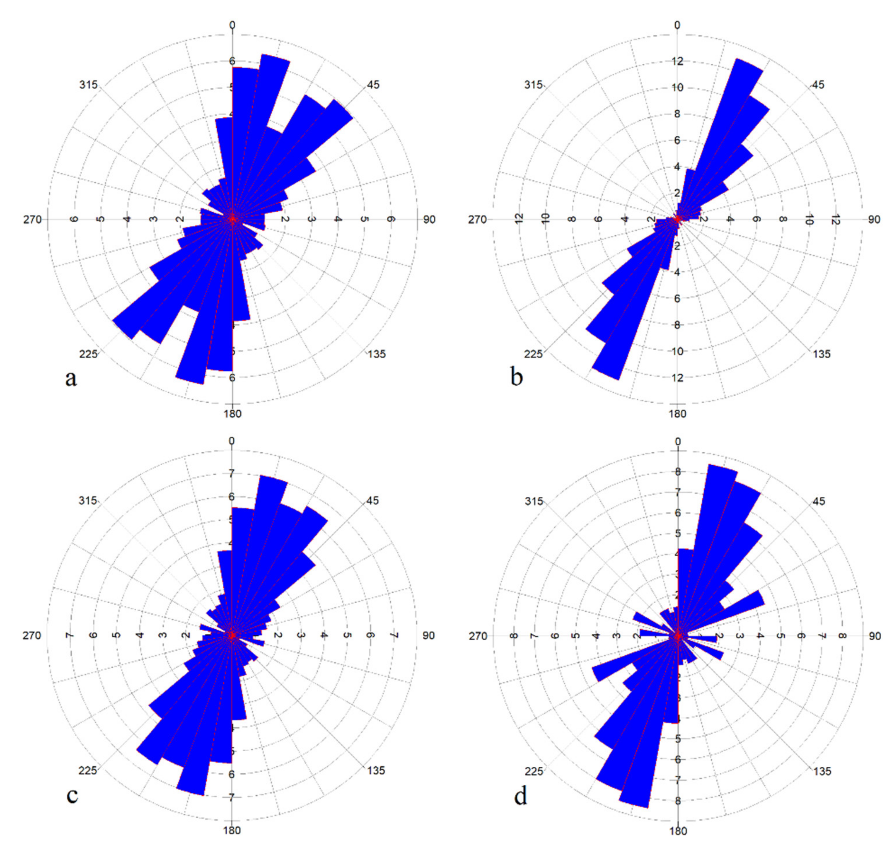
4.2.1. Lineaments Extraction

O’Leary et al. (1976) defined the term “lineaments” as a simple or composite linear feature of a surface for which its parts are aligned in a rectilinear or slightly curvilinear relationship and differs from the pattern of adjacent features and probably reflects some subsurface phenomena [72]. Faults, fractures, and large crush zones are formed by extension or compression processes and are considerable and fundamental factors on ore mineral deposition. Areas with concentrations or intersections of these structures could be suitable for the penetration of magma, ore-forming solutions, and, afterward, mineralization [73]. In other words, a detailed geological study imperatively means acquiring knowledge of present structural information, principally the lineaments [74]. The significance of lineaments is also manifested by their localization often close to several mineralogical deposits [75].
Several studies have been based on Sentinel-2 MSI for the detection of lineaments [76,77,78,79]. According to Bentahar et al. (2020), Sentinel-2 MSI allows extracting more lineaments and extraction of the smallest structural lineaments [79].
Lineament extraction methods can be conducted by using manual photointerpretation by an expert, semi-automatic detection using computer vision techniques, and automatic methods. Automatic methods have resulted in a more efficient lineament extraction process [43,80,81,82,83]. The main steps of lineaments extraction are mentioned below:
  • Applying principal component analysis (PCA) and choosing PC1 to recognize lines;
  • Filter operations using Directional filter with azimuths of 0°, 45°, 90°, and 135°;
  • Automatic lineaments extraction using LINE module in the PCI Geomatica software;
  • Merging lineaments obtained from azimuths of 0°, 45°, 90°, and 135°;
  • Lineament mapping.

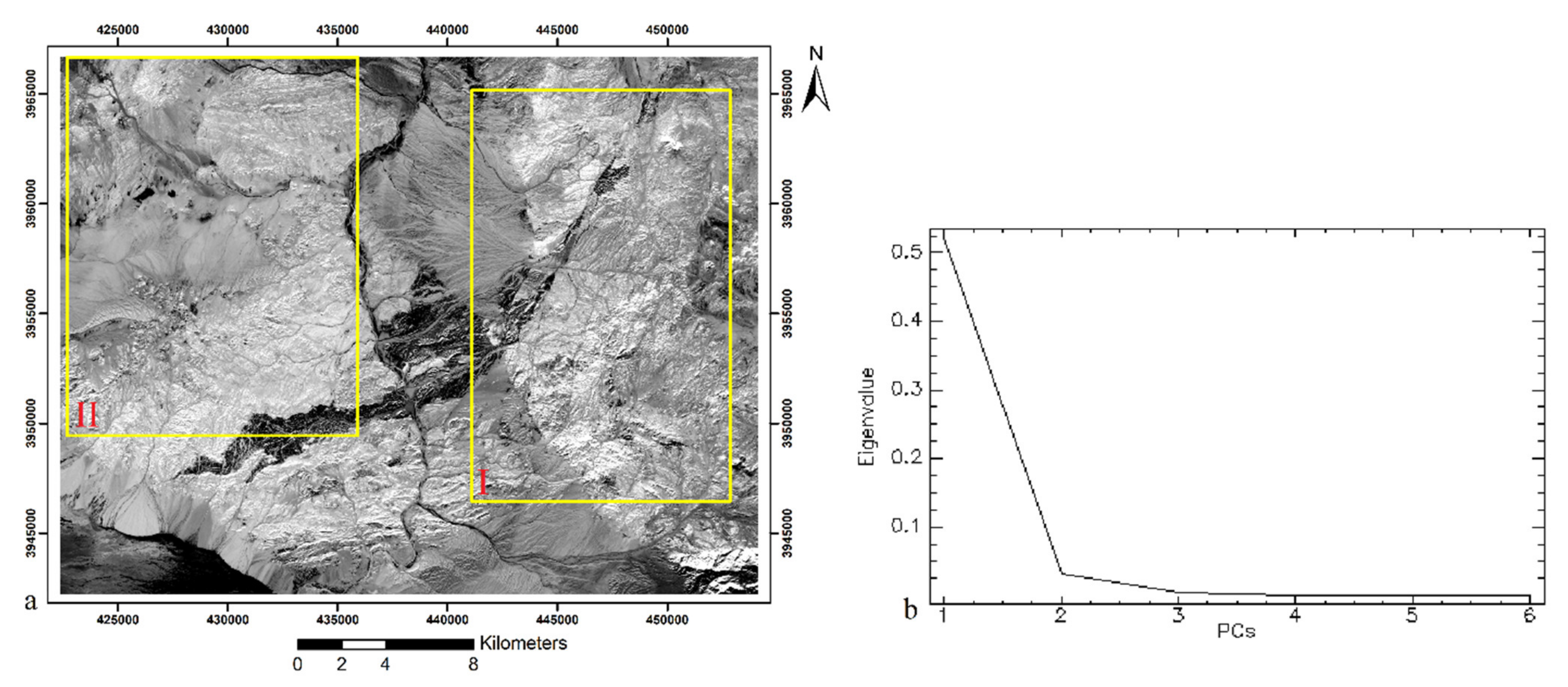
Principal Component Analysis

PCA (Pearson, 1901) is a statistical method that has the advantage of compressing information contained in initial bands into new bands called principal components (PCs) [84,85,86]. This method has been commonly used in lithological mapping and lineament extraction [79]. The PCA method can reduce redundancy in different bands, which can obtain aimed dimension reduction [87], isolation of noise, and enhancement of the targeted information in the image [88]. Each PC can reflect the maximum information of the original variable, and the information contained therein is not repeated.

Filter Operations

Filter operations were used to emphasize or de-emphasize spatial frequency in the image. This frequency can be attributed to the presence of the lineaments in the area. In other words, the filtering operator can sharpen the boundary that exists between adjacent units. A directional filter is a first-order derivative edge enhancement filter that selectively enhances image features possessing specific direction components (gradients) [89]. Directional filters are used strictly for the structural analysis. These filters improve the perception of lineaments, causing an optical effect of shade worn on the image as if it was illuminated by light grazing [78].

PCI Geomatica Software

The automatic extraction of the lineaments was carried out by algorithm LINE EXTRACTION of the PCI Geomatica software [80], which is a widely used module for automatic lineament extraction. The LINE module of PCI Geomatica software extracts linear features from an image and records polylines in vector segments by two main steps, namely edge detection and line detection, and using six parameters [43]:
Edge detection
  • RADI (filter radius) (in pixels): The radius of the filter that is used in contours detection. Values between 3 and 8 are recommended in order to avoid introducing noise;
  • GTHR (Edge Gradient Threshold): The value of the gradient to be taken as the threshold in contour detection (between 0 and 255). Values between 10 and 70 are acceptable;
  • Line detection;
  • LTHR (Curve Length Threshold) (in pixels): The minimum length of a curve to be taken as the lineament (a value of 10 is suitable);
  • FTHR (Line Fitting Threshold) (In pixels): The tolerance allowed in the curve fitting (results of the previous parameter) to form a polyline. Values between 2 and 5 are recommended;
  • ATHR (Angular Difference Threshold) (In degree): Defines the angle not to be exceeded between two polylines to be linked. Values between 3 and 20 are suitable;
  • DTHR (Linking Distance Threshold) (In pixels): The maximum distance between two polylines to be linked. Values between 10 and 45 are acceptable.

4.2.2. Iron Mineralization and Alteration Detection

Lowell and Guilbert (1970) described the San Manuel-Kalamazoo deposit and compared the results with 27 other porphyry-Cu deposits. According to this model, four alteration zones were introduced, which are often used for porphyry-Cu exploration. As shown in Figure 3, the zones in this model from the center to the outside are potassic, phyllic, argillic, and propylitic zones [90,91].
After presenting the Lowell–Guilbert model, some porphyry-Cu deposits were recognized to be associated with intrusive rocks posessing low silica. Hollister (1975) introduced this model and called it the diorite model, although the host pluton may be syenite, monzonite, and diorite [92].
Diorite’s model differs from the Lowell–Guilbert model. In the Diorite model, sulfur concentrations were relatively low in mineralizing fluids. As a result, not all the iron oxides in the host rocks were converted to pyrite, and there are many iron remains in chlorites and biotites. Excess iron tends to occur as magnetite, which may be present in all alteration zones. Therefore, phyllic and argillic alteration zones are usually absent so that the potassic zone is surrounded by the propylitic zone [93,94].

Band Ratio

Band ratios are a very useful method for highlighting certain features or materials that cannot be seen in raw bands [95]. This method was applied to the Sentinel-2 MSI image to detect iron mineralization.

Color Composite

Colors provide more visual and conceptual information of the image. The combination of three black and white images creates a new image that can provide a better interpretation of surface features [96]. This method was used in the ASTER image for better visual interpretation of the alteration areas.

Logical Operator Algorithm

Mars and Rowan (2006) developed two logical operator algorithms based on ASTER-defined band ratios for regional mappings of argillic and phyllic-altered rocks in the Zagros magmatic arc, Iran [97]. Mars (2013) used thermal images in-band ratios to map hydrothermal alterations [98]. The logical operator algorithm presented by Mars (2013) can be the best suited for hydrothermal alteration associated with porphyry-Cu mineralization on a regional scale. The logical operator algorithm performs a series of band ratios for each pixel. Each logical operator determines a true (one) or false (zero) value for each ratio by comparing the band ratio to a predetermined range of threshold values. All of the ratios in the algorithm have to be true for a value of one to be assigned to the byte image; otherwise, a zero value is produced. Thus, a byte image consisting of zeros and ones is produced with each algorithm [97]. Due to the geological settings in the study area, the logical operator algorithm was applied to the Aster image to map alterations.

4.2.3. Generation of The Geological Layer

The geological layer is created by combining rock units, faults, and alterations using the K-nearest neighbor (KNN) algorithm. The 1:100,000 scale map of Abrisham-Rud has complex and multistage geological settings, and some units may not have outcrop, whereas this scale does not pose a problem for this study. The layer of rock units was created by using the high value for intrusive rock and intermediate to base units, as well as the low value for other units. In the study area, faults are dense and intersect in different directions. Fault layers were created by buffers at 100 to 500 at 100 m intervals. The alteration layers for each argillic, phyllic, and propylitic (epidote-chlorite) alteration were created by buffers at 100 to 300 at 100 m intervals around the alteration.

K-Nearest Neighbor Algorithm

KNN is a non-parametrically supervised algorithm designed to solve regression and classification problems [99]. KNN is the fundamental and the simplest classification technique when there is little or no prior knowledge about the distribution of data [100]. This algorithm is quite successful when a large training data set [101] and many geological studies are provided [102,103,104,105,106].
KNN classifies objects based on the closest training examples in the feature space [107,108]. In order to classify or predict a new case, KNN relies on finding similar cases in training data. These cases are classified by voting for neighbor classes [109]. The optimal choice of the number of neighbors “K” depends on the metrics used for classification and regression purposes [109]. Thus, KNN algorithm predicts the target class through three steps [101,110]: (1) preparing the dataset consists of training, test, and feature; (2) measuring the distances between each test data and all training data depending on the weight values of each individual; and (3) finding “K” the neighbors nearest to the test data from training data based on distance and weight measurements.
The most common and simple distance metrics are Euclidean, Manhattan, and Minkowski. The Minkowski distance is generally a more complete form of distance metrics and is calculated based on Equation (9):
Minkowski   Distance = i = 1 k x i y i λ λ ,
where x and y are points to calculate the distance, k is the number of neighbors, and λ is the order of the Minkowski distance, which contains values greater than zero. Thus, where λ = 2, the Minkowski distance is equivalent to the Manhattan distance, and where λ = 1, it is equivalent to the Euclidean distance. The Manhattan distance is usually preferred over the more common Euclidean distance when there is high dimensionality in the data set [111].
In this study, the Manhattan distance was used as the nearest neighbor classifier, and weights were calculated on Equation (10) based on the distance from the target to predict in a neighborhood:
weighted   Manhattan   Distance = i = 1 k W i x i y i ,
where W is the weights for each nearest neighbor, 0 < Wi < 1 and i = 1 k Ww i = 1 .

5. Result and Discussion

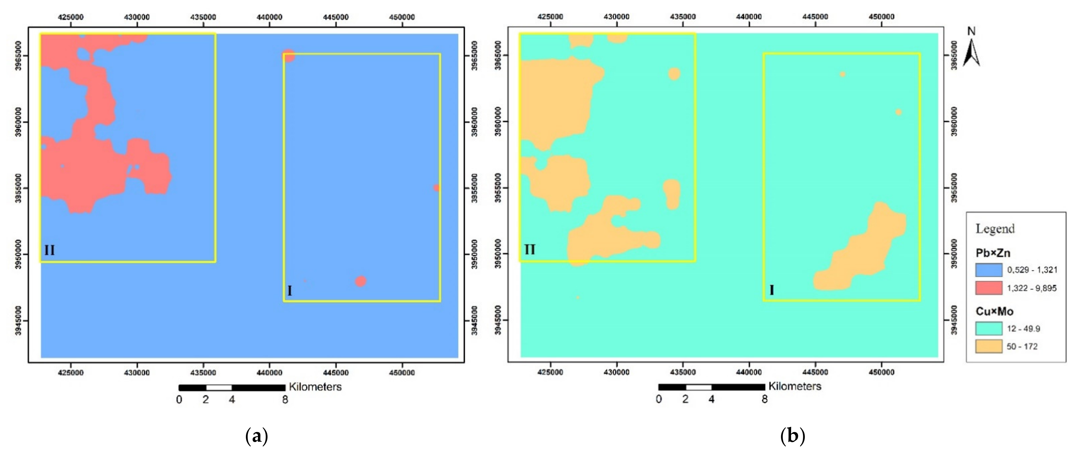
5.1. Zonality Method

Table 1 shows the calculation of background and threshold values, as well as the Clark values for supra-ore (Pb and Zn) and sub-ore (Cu and Mo) elements in the study area.
Figure 4 shows the anomaly map of multiplicative geochemical halos of the supra-ore and sub-ore (Cu × Mo) elements. As shown in Figure 4, zones I and II have been considered to predict erosional levels, and they create the geological layer. As shown in Figure 4, zone I mostly implied sub-ore (Cu and Mo) elements, and zone II included both supra-ore (Pb and Zn) and sub-ore (Cu and Mo) elements. The co-existence of both supra-ore and sub-ore elements’ local maxima implies blind mineralization [20].
The geochemical and geometrical similarity of genetically similar orebodies, the uniformity of ore and halo, and the tentative nature of geological and economic boundaries are all crucial for considering mining geochemical models. In addition, the vertical geochemical zonality index and their spatial associations with particular geological and geochemical factors are important aspects of mineral distributions for exploration and insight into ore geometry. The vertical geochemical zonality index could be used to estimate the erosional level of porphyry-Cu deposits [2,3]. In order to identify the erosional level in zones I and II, the presented models by Ziaii (1996) and Ziaii et al. (2009) were used [2,67].
Ziaii (1996) introduced the vertical zonality model for porphyry-Cu deposits using areal productivity and the zonality index (Equation (6)) based on porphyry-Cu deposits in Kazakhstan, Bulgaria, Armenia, and Iran (Figure 5a). The vertical variations in three zonality indices associated with porphyry-Cu deposits in areas of the same landscape-geochemical conditions in different countries are shown in Figure 5a. Values of each zonality index decrease downward uniformly despite considerable differences in local geological settings of individual porphyry-Cu deposits, suggesting the existence of uniform vertical zonality in primary halos of porphyry-Cu deposits [2,6,71]. Therefore, vertical variations in the indices allow the distinction of mineralization levels and their primary halos (supra ore, upper-ore, ore, lower-ore, and sub-ore) [6,22,24].
Moreover, it can be deduced from Figure 5a that similar values of the zonality index imply similar depths of mineralization and primary halos within an ore field. Thus, primary halos of mineral deposits at different depths are characterized by specific values of the zonality index. The practical exploration significance of the zonality index is for the recognition of erosional surfaces representing vertical levels of geochemical anomalies. Concerning the present erosional level, high values of the zonality index imply the presence of sub-cropping to BM, whereas low values of the index imply outcropping or already eroded deposits [14].
The values of areal productivity, mineralization coefficient, and zonality indices were introduced by Solovov (KS) and Grigorian (KG) in two zones (Table 2). The values of (Ks) in zones I and II are equal to 0.18 and 26.57, respectively. Considering the presented model by Ziaii (1996) [71], zones I and II are ZDM and BM, respectively (Figure 5a).
Ziaii et al. (2009) introduced the geochemical model for porphyry-Cu deposits in Aktogy (Kazakhstan), Asarel (Bulgaria), Tekhut (Armenia), and Sungun (Iran) using mineralization coefficient and zonality index (Figure 5b) [2]. This plot shows the depth of mineralization versus the zonality index (KG). Despite considerable differences in geological settings, the linear relationship suggests the existence of a quantitatively uniform vertical geochemical zonality in the structure of primary halos of the deposits.
In this study, the values of (KG) in zones I and II are equal to 0.71 and 28.23, respectively (Table 2). According to the presented model by Ziaii et al. (2009), erosional levels in zone I and II are nearly similar to Astamal and Songun 2 areas, respectively (Figure 5b). Based on the previous studies, Sungun 2 and Astamal areas have been recognized as BM and ZDM, respectively [2].
Therefore, the results of the introduced models by Ziaii (1996) and Ziaii et al. (2009) confirm each other in identifying the erosional level in each zone [2,71].

5.2. Remote Sensing

Lineaments Extraction

The procedure of lineament extraction was accomplished in this manner: the PCA image of six Sentinel-2 MSI bands (bands 2, 3, 4, 8, 11, and 12), as shown in Figure 6a. PC1 explains the largest amount of eigenvalue among six bands. PC1 with the loading of the same signs represents overall brightness in all bands [14], and it shows that the albedo is related largely to the topographic features [76] (Figure 6b). Then, a directional filter was applied using 3 × 3 kernels in four directions with azimuths of 0°, 45°, 90°, and 135°. By using these azimuths, this filter visually enhances edges striking N-S, NE-SW, E-W, and NW-SE, respectively.
The sum of the directional filter kernel arrays is zero. The result is that areas with uniform pixel values are zeroed in the output image, while those with variable pixel values are presented as bright edges. In PCI Geomatica software, differences in the values of six parameters of edge and line detection indicate the differences of opinion among researchers. The values proposed by Adiri et al. (2017) were used [43]. Finally, the lineaments obtained from azimuths of 0°, 45°, 90°, and 135° were merged, and the repetitive segments and non-geological lineaments (river, road, etc.) were deleted.
Lineaments and lineaments density maps in two zones were demonstrated in Figure 7. Lineament density was used to find the correlation between the concentration of lineaments and the distribution of existing faults in the study area (Figure 7). In two zones, this comparison proved that the fault is well related to lineament density in most areas. These areas were generally recognized in the middle-upper Eocene units and intrusive rocks.
Lineament orientation allows identifying the most frequent directions of lineaments, and they can be compared with directions related to the existing faults [43]. As shown in Figure 8, in zones I and II, the directions of the lineaments correspond to existing faults.
Lineaments may be formed, for example, by structural alignment, geomorphologic consequences, structural weaknesses, faults, valleys, rivers, the boundaries between the different lithological units, vegetation cover, and artificial objects (road, bridge, etc.) [43]. In this study, due to the importance of faults in porphyry-Cu mineralization [6], the faults obtained from the geological map were used to create a geological layer.

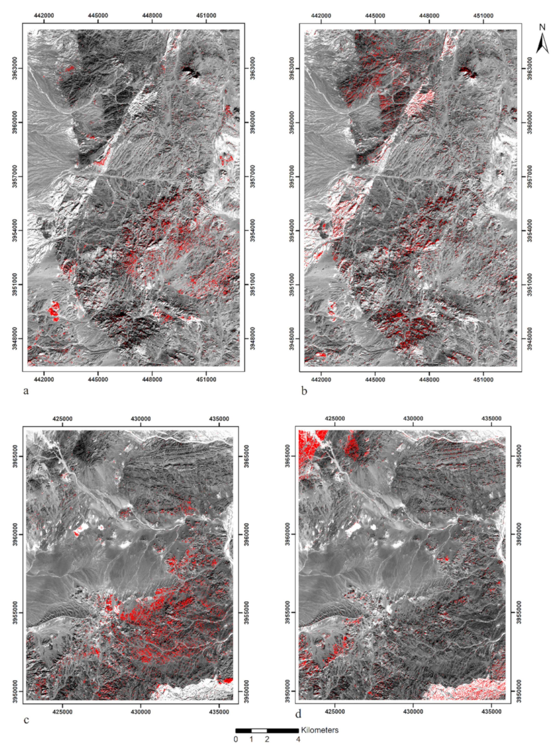
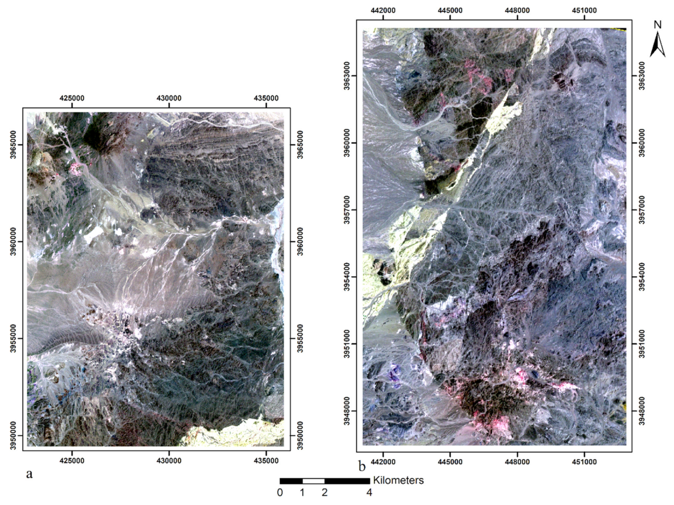
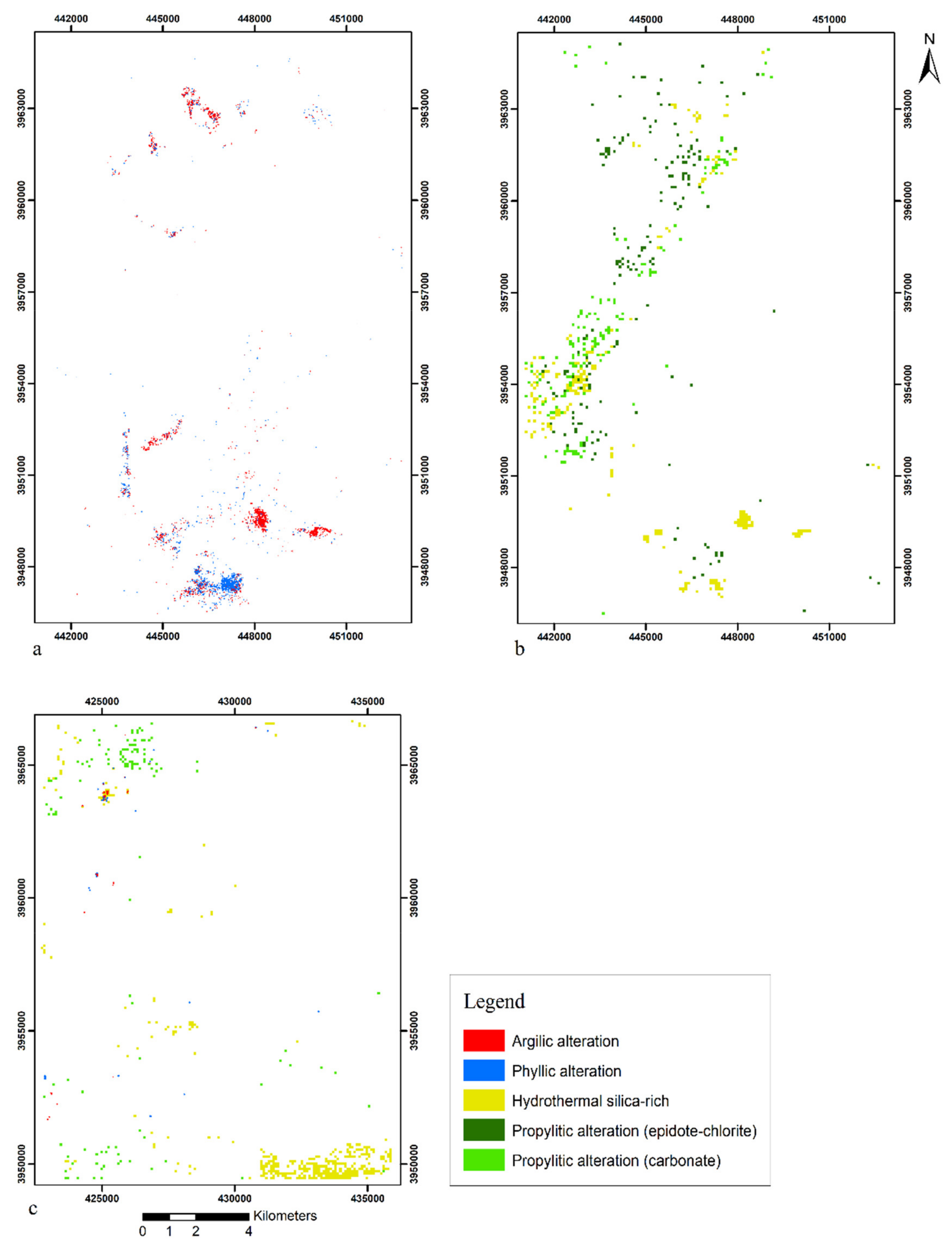
5.3. Iron Mineralization and Alteration Detection

The results of the band ratio applied to Sentinel-2 MSI were shown in Figure 9. According to the rock units in the studied zones and Porphyry-Cu alterations zones, iron mineralization is dispersed and dense in two zones (Figure 9), which is well identified in areas containing volcanic and intrusive rocks. In the south of zone I, which includes intrusive rock consisting of monzodiorite and monzogabbro, iron mineralization is well recognized.
In ASTER, false-color composites of SWIR bands were used for better visual interpretation of the alteration areas. Empirical combinations have shown that an image with a false-color composite (band 4 in red, band 6 in green, and band 8 in blue) is the most suitable color composite for identifying alteration areas in porphyry-Cu deposits. As shown in Figure 10, areas with the propylitic alteration are shown in green to dark green based on the alteration intensity, and areas with the argillic and phyllic alteration are shown in white and pink to red. This is due to the high reflectivity of alunite, kaolinite, and muscovite minerals in band 4 compared to bands 6 and 8.
Geological settings in the study area have made it difficult to identify some alterations, especially in zone II. Rocks containing hydrous quartz, chalcedony, opal, and amorphous silica (hydrothermal silica-rich rocks); calcite-dolomite and epidote-chlorite (propylitic); alunite-pyrophyllite-kaolinite (argillic); and sericite-muscovite (phyllic) were mapped using ASTER and logical operator algorithms (Figure 11). It is observed that Mars (2013) used images that have to differ in correction levels from the images used in this paper. Mars (2013) used “and (b4 gt 260)” to remove the black pixel [94], but in the images that have been used in this paper, the pixel has no value higher than 260. Thus, “and” in the algorithm causes the result to be zero (Table 3).
Although not all alterations are associated with ore bodies and not all ore bodies are accompanied by alteration, the presence of altered rocks is a valuable indicator of possible deposits [112]. Kaolinite is mostly related to weathering feldspars, and epidote can be related to regional metamorphism. Kaolinite and epidote anomalies can have genesis related to deposit when they have a close relationship with muscovite anomalies [65].
Due to intrusive rocks, there is a possibility of the diorite model in the south of zone I. In this area, propylitic alteration (epidote–chlorite) was identified less than other parts of zone I, and argillic and phyllic alterations are well-identified around these intrusive rocks. It should be noted that all intrusive rocks have not shown alterations, which could be due to erosion or geological settings. Furthermore, alterations have been identified in other areas of zone I, which could imply mineralization areas or presence of minerals associated with alterations. In zone II, propylitic alteration (epidote–chlorite) was not identified, but argillic and phyllic alterations were detected in part of the studied area. Therefore, because of the absence of the alterations, it is not reasonable to create a geological layer in this zone.

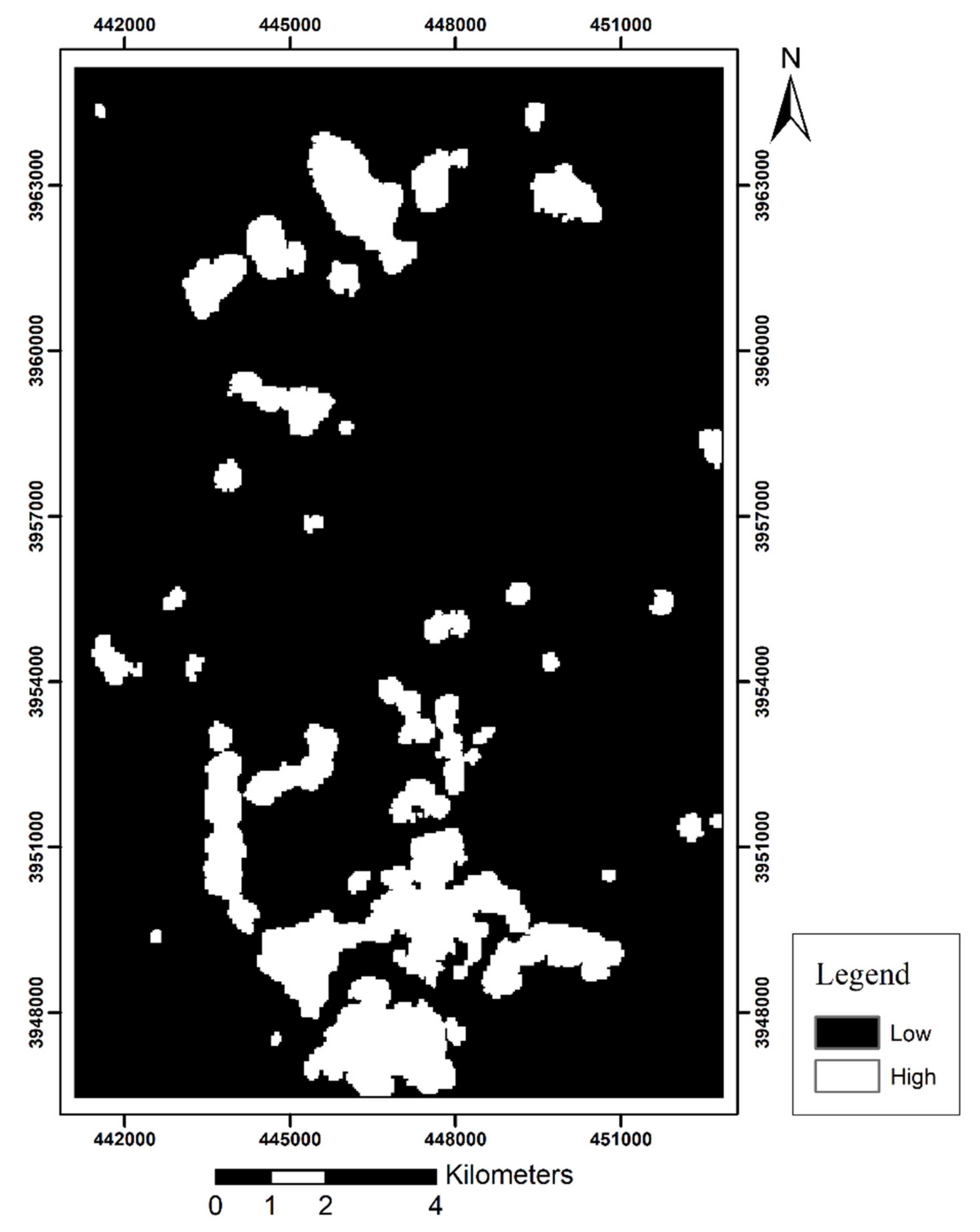
5.4. Geological Layer

Rock units, faults, and alterations layers were combined by using the KNN algorithm and the geological layer, as shown in Figure 12. In this procedure, faults and alterations have an important role in mapping high potential areas. The density and intersection of faults and the extent of alterations represent these areas. Considering the geological layer, the detected areas as high potential could be related to mineralization or not. These areas can be compared to anomalous areas obtained by using the zonality method. As a result, more parts of the geological layer map were detected as high potential in comparison to the zonality method. However, the results of both methods confirm each other in the south of zone I. The geological layer and mineralogical investigation cannot identify erosional levels. In addition, mineralogy is not economical for application on a regional scale. In the study area, it is not recommended.
Unlike the geological layer, the application of the zonality method in mineral prospecting allows further interpretation about whether delineated desirable areas are attractive for the exploration of ZDM or BM deposits.
This comparison demonstrates that the zonality method for detecting anomalous areas is more powerful than the geological layer.

6. Conclusions

The traditional zonality method has been used in the exploration of porphyry-Cu deposits for many years and is an effective method for the distinction between sub-ore and supra-ore halos, prediction of the erosional level of mineralization, and exploration of blind mineral deposits.
Utilizing the zonality method, the geochemical maps of multiplicative haloes were mapped. In the east of the study area, multiplicative haloes of sub-ore elements (Cu and Mo) were observed, and these represent zone dispersed mineralization. In the northwest, both multiplicative supra-ore (Pb and Zn) and sub-ore (Cu and Mo) element haloes existed, and these imply blind mineralization. Thus, zones I and II, which are located in the east and northwest of the study area, were selected for calculating erosional levels and for creating the geological map. Zonality indices introduced by Solovov (1987) (Ks) and Beus and Grigorian (1977) (KG) were calculated in zones I and II [12,22]. The (Ks) values were equal to 0.18 and 26.57 in zones I and II, respectively; moreover, (KG) values in zones I and II were equal to 0.71 and 28.23, respectively. Then, the presented models by Ziaii (1996) and Ziaii et al. (2009) were considered for identifying erosional levels in these zones [2,67]. Due to these models, zones I and II were recognized as ZDM and BM, respectively. Therefore, the zonality method was successfully applied in the identification of anomalous areas, separate BM from ZDM, and predicted erosional levels.
The results of the zonality method were compared to the geological layer, which was created by rock units, faults, and alterations by using the KNN algorithm. Each of these layers plays an important role in prospecting and exploring mineral deposits. Thus, high potential areas can be identified by combining these layers. For zones I and II, rock units and faults were identified from the geological map, and the alterations were detected using ASTER images and logical operator algorithms. It was observed that the alterations layers had a significant contribution in constructing the geological layer. The alteration zones of porphyry-Cu deposits include propylitic (chlorite and epidote), argillic (alunite and kaolinite), and phyllic (sericite and muscovite), and they are important for identifying possible areas associated with porphyry-Cu systems. These alterations were detected in zone I, especially around the intrusive rocks in the S of this zone. In zone II, only argillic and phyllic alterations were identified in part of the studied area. Due to the lack of alteration in zone II, the geological layer was created only in zone I. Comparing the results of the two methods showed that more parts of the geological layer map were highlighted as having high potential. These high potential areas could be related to mineralization or not; in other words, the geological layer cannot separate BM from ZDM. However, the results of both methods correspond to each other in the south of zone I. In other, the geological layer is unable to recognize erosional levels. Therefore, mineralogy investigation is required, which is not recommended to apply on a regional scale because of its high cost. It could be concluded that the geological layer, which is based on alteration, cannot help geochemists in separating BM from ZDM and in predicting erosional levels.

Author Contributions

M.Z. and M.R.G. conceived and designed the study and wrote the initial draft of the manuscript. M.R.G. and M.A. collected the samples and conducted sample preparation for analytical work. M.R.G. and M.Z. analyzed the data and conducted processing graphic and analytical work. T.T. revised and corrected the final version. All authors have read and agreed to the published version of the manuscript.

Funding

This research received no external funding.

Data Availability Statement

All information is collected by the researchers of this article and is not accessible anywhere.

Acknowledgments

This research was funded by the School of Mining, Petroleum and Geophysics Engineering at the Shahrood University of Technology. Laboratory research was carried out within the framework of the Tomsk Polytechnic University Development Program. Authors are thankful to anonymous reviewers and the editor for constructive criticisms and useful suggestions on the paper.

Conflicts of Interest

The authors declare no conflict of interest.

References

  1. Fersman, A.E. Geochemical and Mineralogical Methods of Prospecting for Mineral Deposits; Academy of Science: Moscow, Russia, 1939. (In Russian) [Google Scholar]
  2. Ziaii, M.; Pouyan, A.A.; Ziaei, M. Neuro-fuzzy modelling in mining geochemistry: Identification of geochemical anomalies. J. Geochem. Explor. 2009, 100, 25–36. [Google Scholar] [CrossRef]
  3. Ziaii, M.; Ardejani, F.D.; Ziaei, M.; Soleymani, A.A. Neuro-fuzzy modeling based genetic algorithms for identification of geochemical anomalies in mining geochemistry. Appl. Geochem. 2012, 27, 663–676. [Google Scholar] [CrossRef]
  4. Hamedani, M.L.; Plimer, I.R.; Xu, C. Orebody Modelling for Exploration: The Western Mineralisation, Broken Hill, NSW. Nat. Resour. Res. 2012, 21, 325–345. [Google Scholar] [CrossRef]
  5. Grigorian, S.V. Secondary Lithochemical Haloes in Prospecting for Hidden Mineralization; Nedra Publishing House: Moscow, Russia, 1985. (In Russian) [Google Scholar]
  6. Grigorian, S.V. Mining Geochemistry; Nedra Publishing House: Moscow, Russia, 1992. (In Russian) [Google Scholar]
  7. Ziaii, M.; Abedi, A.; Ziaei, M. Prediction of hidden ore bodies by new integrated computational model in marginal Lut region in east of Iran. Proc. Explor. 2007, 7, 957–961. [Google Scholar]
  8. Ziaii, M.; Pouyan, A.A.; Ziaei, M. Geochemical anomaly recognition using fuzzy C-means cluster analysis. Wseas Trans. Syst. 2006, 5, 2424–2429. [Google Scholar]
  9. Li, H.; Wang, Z.; Li, F. Ideal models of superimposed primary halos in hydrothermal gold deposits. Geochem. Explor. 1995, 55, 329–336. [Google Scholar] [CrossRef]
  10. Li, H.; Zhang, G.Y.; Yu, B. Tectonic Primary Halo Model and the Prospecting Effect During Deep Buried Ore Prospecting in Gold Deposits; Geological Publishing House: Beijing, China, 2006. [Google Scholar]
  11. Yongqing, C.; Pengda, Z. Zonation in primary halos and geochemical prospecting pattern for the Guilaizhuang gold deposit, eastern China. Nonrenew. Resour. 1998, 7, 37–44. [Google Scholar] [CrossRef]
  12. Beus, A.A.; Grigorian, S.V. Geochemical Exploration Methods for Mineral Deposits; Applied Publishing Ltd.: Wilmette, IL, USA, 1977. [Google Scholar]
  13. Yongqing, C.; Jingning, H.; Zhen, L. Geochemical characteristics and zonation of primary halos of pulang porphyry copper deposit, Northwestern Yunnan Province, Southwestern China. J. China Univ. Geosci. 2008, 19, 371–377. [Google Scholar] [CrossRef]
  14. Ziaii, M.; Carranza, E.J.M.; Ziaei, M. Application of geochemical zonality coefficients in mineral prospectivity mapping. Comput. Geosci. 2011, 37, 1935–1945. [Google Scholar] [CrossRef]
  15. Harraz, H.Z.; Hamdy, M.M. Zonation of primary haloes of Atud auriferous quartz vein deposit, Central Eastern Desert of Egypt: A potential exploration model targeting for hidden mesothermal gold deposits. J. Afr. Earth Sci. 2015, 101, 1–18. [Google Scholar] [CrossRef]
  16. Safari, S.; Ziaii, M.; Ghoorchi, M. Integration of singularity and zonality methods for prospectivity map of blind mineralization. Int. J. Min. Geo Eng. 2016, 50, 189–194. [Google Scholar]
  17. Imamalipour, A.; Mousavi, R. Vertical geochemical zonation in the Masjed Daghi porphyry copper-gold deposit, northwestern Iran: Implications for exploration of blind mineral deposits. Geochem. Explor. Environ. Anal. 2018, 18, 120–131. [Google Scholar] [CrossRef]
  18. Imamalipour, A.; Karimlou, M.; Hajalilo, B. Geochemical zonality coefficients in the primary halo of Tavreh mercury prospect, northwestern Iran: Implications for exploration of listwaenitic type mercury deposits. Geochem. Explor. Environ. Anal. 2019, 19, 347–357. [Google Scholar] [CrossRef]
  19. Safari, S.; Ziaii, M.; Ghoorchi, M.; Sadeghi, M. Application of concentration gradient coefficients in mining geochemistry: A comparison of copper mineralization in Iran and Canada. J. Min. Environ. 2018, 9, 277–292. [Google Scholar]
  20. Ziaii, M.; Safari, S.; Timkin, T.; Voroshilov, V.; Yakich, T. Identification of geochemical anomalies of the porphyry–Cu deposits using concentration gradient modelling: A case study, Jebal-Barez area, Iran. J. Geochem. Explor. 2019, 199, 16–30. [Google Scholar] [CrossRef]
  21. Safari, S.; Ziaii, M. Evaluation of geochemical anomalies in kerver deposit. Iran. J. Min. Eng. IRJME 2019, 14, 76–91. (In Persian) [Google Scholar]
  22. Solovov, A.P. Geochemical Prospecting for Mineral Deposits; Mir: Moscow, Russia, 1987. (In Russian) [Google Scholar]
  23. Baranov, E.V. Endogenetic Halos Associated with Massive Sulphide Deposits; Nedra Publishing House: Moscow, Russia, 1987. (In Russian) [Google Scholar]
  24. Solovov, A.P.; Arkhipov, A.Y.; Bugrov, V.A. Guidebook on Geochemical Exploration of Mineral Resources; Nedra Publishing House: Moscow, Russia, 1990. (In Russian) [Google Scholar]
  25. Liu, L.M.; Peng, S.L. Prediction of hidden ore bodies by synthesis of geological, geophysical and geochemical information based on dynamic model in Fenghuangshan ore field, Tongling district, China. J. Geochem. Explor. 2004, 81, 81–98. [Google Scholar] [CrossRef]
  26. Asadi, H.H.; Sansoleimani, A.; Fatehi, M.; Carranza, E.J.M. An AHP–TOPSIS Predictive Model for District-Scale Mapping of Porphyry Cu–Au Potential: A Case Study from Salafchegan Area (Central Iran). Nat. Resour. Res. 2016, 25, 417–429. [Google Scholar] [CrossRef]
  27. Yousefi, M.; Carranza, E.J.M. Union score and fuzzy logic mineral prospectivity mapping using discretized and continuous spatial evidence values. J. Afr. Earth Sci. 2017, 128, 47–60. [Google Scholar] [CrossRef]
  28. Shabankareh, M.; Hezarkhani, A. Application of support vector machines for copper potential mapping in Kerman region, Iran. J. Afr. Earth Sci. 2017, 128, 116–126. [Google Scholar] [CrossRef]
  29. Pazand, K.; Hezarkhani, A. Predictive Cu porphyry potential mapping using fuzzy modelling in Ahar–Arasbaran zone, Iran. Geol. Ecol. Landsc. 2018, 2, 229–239. [Google Scholar] [CrossRef] [Green Version]
  30. Mars, J.C.; Robinson, G.R., Jr.; Hammarstrom, J.M.; Zürcher, L.; Whitney, H.; Solano, F.; Gettings, M.; Ludington, S. Porphyry copper potential of the United States southern basin and range using ASTER data integrated with geochemical and geologic datasets to assess potential near-surface deposits in well-explored permissive tracts. Econ. Geol. 2019, 114, 1095–1121. [Google Scholar] [CrossRef]
  31. Ford, A. Practical implementation of random forest-based mineral potential mapping for porphyry Cu–Au mineralization in the Eastern Lachlan Orogen, NSW, Australia. Nat. Resour. Res. 2020, 29, 267–283. [Google Scholar] [CrossRef]
  32. Voroshilov, V.G. Anomalous structures of geochemical fields of hydrothermal gold deposits: Formation mechanism, methods of geometrization, typical models, and forecasting of ore mineralization. Geol. Ore Depos. 2009, 51, 1–16. [Google Scholar] [CrossRef]
  33. Shirazy, A.; Hezarkhani, A.; Timkin, T.; Shirazi, A. Investigation of Magneto-/Radio-Metric Behavior in Order to Identify an Estimator Model Using K-Means Clustering and Artificial Neural Network (ANN) (Iron Ore Deposit, Yazd, IRAN). Minerals 2021, 11, 1304. [Google Scholar] [CrossRef]
  34. Shirazy, A.; Ziaii, M.; Hezarkhani, A.; Timkin, T.V.; Voroshilov, V.G. Geochemical behavior investigation based on K-means and artificial neural network prediction for titanium and zinc, Kivi region, Iran. Bull. Tomsk Polytech. Univ. Geo Assets Eng. 2021, 332, 113–125. [Google Scholar]
  35. Carranza, E.J.M. Geologically Constrained Mineral Potential Mapping: Examples from the Philippines. Ph.D. Thesis, Technische Universiteit Delft, Delft, The Netherlands, 2002. [Google Scholar]
  36. Adiri, Z.; Lhissou, R.; El Harti, A.; Jellouli, A.; Chakouri, M. Recent advances in the use of public domain satellite imagery for mineral exploration: A review of Landsat-8 and Sentinel-2 applications. Ore Geol. Rev. 2020, 117, 103332. [Google Scholar] [CrossRef]
  37. Cox, D.P.; Singer, D.A. Mineral deposit models. U.S. Geol. Surv. Bull. 1693, 1986, 393. [Google Scholar]
  38. Yumul, G.P., Jr.; Dimalanta, C.B.; Gabo-Ratio, J.A.S.; Armada, L.T.; Queaño, K.L.; Jabagat, K.D. Mineralization parameters and exploration targeting for gold—Copper deposits in the Baguio (Luzon) and Pacific Cordillera (Mindanao) Mineral Districts, Philippines: A review. J. Asian Earth Sci. 2020, 191, 104232. [Google Scholar] [CrossRef]
  39. Zarasvandi, A.; Liaghat, S.; Zentilli, M. Geology of the Darreh-Zerreshk and Ali-Abad porphyry copper deposits, central Iran. Int. Geol. Rev. 2005, 47, 620–646. [Google Scholar] [CrossRef]
  40. Sillitoe, R.H. Porphyry Copper Systems. Econ. Geol. 2010, 105, 3–41. [Google Scholar] [CrossRef] [Green Version]
  41. Mirzaie, A.; Bafti, S.S.; Derakhshani, R. Fault control on Cu mineralization in the Kerman porphyry copper belt, SE Iran: A fractal analysis. Ore Geol. Rev. 2015, 71, 237–247. [Google Scholar] [CrossRef]
  42. Habibkhah, N.; Hassani, H.; Maghsoudi, A.; Honarmand, M. Application of numerical techniques to the recognition of structural controls on porphyry Cu mineralization: A case study of Dehaj area, Central Iran. Geosystem Eng. 2020, 23, 159–167. [Google Scholar] [CrossRef]
  43. Adiri, Z.; El Harti, A.; Jellouli, A.; Lhissou, R.; Maacha, L.; Azmi, M.; Zouhair, M.; Bachaoui, E.M. Comparison of Landsat-8, ASTER and Sentinel 1 satellite remote sensing data in automatic lineaments extraction: A case study of Sidi Flah-Bouskour inlier, Moroccan Anti Atlas. Adv. Space Res. 2017, 60, 2355–2367. [Google Scholar] [CrossRef]
  44. Azizi, H.; Tarverdi, M.A.; Akbarpour, A. Extraction of hydrothermal alterations from ASTER SWIR data from east Zanjan, northern Iran. Adv. Space Res. 2010, 46, 99–109. [Google Scholar] [CrossRef]
  45. Mielke, C.; Boesche, N.K.; Rogass, C.; Kaufmann, H.; Gauert, C.; De Wit, M. Spaceborne mine waste mineralogy monitoring in South Africa, applications for modern push-broom missions: Hyperion/OLI and EnMAP/Sentinel-2. Remote Sens. 2014, 6, 6790–6816. [Google Scholar] [CrossRef] [Green Version]
  46. Van der Werff, H.; Van der Meer, F. Sentinel-2A MSI and Landsat 8 OLI provide data continuity for geological remote sensing. Remote Sens. 2016, 8, 883. [Google Scholar] [CrossRef] [Green Version]
  47. Pour, A.B.; Hashim, M.; Park, Y.; Hong, J.K. Mapping alteration mineral zones and lithological units in Antarctic regions using spectral bands of ASTER remote sensing data. Geocarto Int. 2018, 33, 1281–1306. [Google Scholar] [CrossRef]
  48. Zhang, N.; Zhou, K. Identification of hydrothermal alteration zones of the Baogutu porphyry copper deposits in northwest China using ASTER data. J. Appl. Remote Sens. 2017, 11, 015016. [Google Scholar] [CrossRef]
  49. Safari, M.; Maghsoudi, A.; Pour, A.B. Application of Landsat-8 and ASTER satellite remote sensing data for porphyry copper exploration: A case study from Shahr-e-Babak, Kerman, south of Iran. Geocarto Int. 2018, 33, 1186–1201. [Google Scholar] [CrossRef]
  50. Testa, F.J.; Villanueva, C.; Cooke, D.R.; Zhang, L. Lithological and hydrothermal alteration mapping of epithermal, porphyry and tourmaline breccia districts in the Argentine Andes using ASTER imagery. Remote Sens. 2018, 10, 203. [Google Scholar] [CrossRef] [Green Version]
  51. Noori, L.; Pour, A.B.; Askari, G.; Taghipour, N.; Pradhan, B.; Lee, C.W.; Honarmand, M. Comparison of different algorithms to map hydrothermal alteration zones using ASTER remote sensing data for polymetallic vein-type ore exploration: Toroud–Chahshirin magmatic belt (TCMB), North Iran. Remote Sens. 2019, 11, 495. [Google Scholar] [CrossRef] [Green Version]
  52. Adiri, Z.; El Harti, A.; Jellouli, A.; Maacha, L.; Azmi, M.; Zouhair, M.; Bachaoui, E.M. Mapping copper mineralization using EO-1 Hyperion data fusion with Landsat 8 OLI and Sentinel-2A in Moroccan Anti-Atlas. Geocarto Int. 2020, 35, 781–800. [Google Scholar] [CrossRef]
  53. Shirazy, A.; Ziaii, M.; Hezarkhani, A.; Timkin, T. Geostatistical and Remote Sensing Studies to Identify High Metallogenic Potential Regions in the Kivi Area of Iran. Minerals 2020, 10, 869. [Google Scholar] [CrossRef]
  54. Zürcher, L.; Bookstrom, A.A.; Hammarstrom, J.M.; Mars, J.C.; Ludington, S.D.; Zientek, M.L.; Dunlap, P.; Wallis, J.C. Tectono-magmatic evolution of porphyry belts in the central Tethys region of Turkey, the Caucasus, Iran, western Pakistan, and southern Afghanistan. Ore Geol. Rev. 2019, 111, 102849. [Google Scholar] [CrossRef]
  55. Orojnia, P. Lithology and provenance of Eocene volcanic rocks in 1:100000 scale map sheet of Abrisham–Roud. Master’s Thesis, Geological Survey and Mineral Explorations of Iran, Tehran, Iran, 2003; p. 140. (In Persian). [Google Scholar]
  56. Mars, J.C. Regional Mapping of Hydrothermally Altered Igneous Rocks along the Urumieh-Dokhtar, Chagai, and Alborz Belts of Western Asia Using Advanced Spaceborne Thermal Emission and Reflection Radiometer (ASTER) Data and Interactive Data Language (IDL) Logical Operators: A Tool for Porphyry Copper Exploration and Assessment: Chapter O in Global Mineral Resource Assessment; Scientific Investigations Report 2010-5090-O; U.S. Geological Survey: Reston, VA, USA, 2014; p. 36.
  57. Nabavi, M.H. An introduction to geology of Iran, Geological Survey and Mineral Explorations of Iran, Tehran; Geological Survey of Iran: Tehran, Iran, 1976. (In Persian) [Google Scholar]
  58. Zürcher, L.; Bookstrom, A.A.; Hammarstrom, J.M.; Mars, J.C.; Ludington, S.; Zientek, M.L.; Dunlap, P.; Wallis, J.C.; Drew, L.J.; Sutphin, D.M.; et al. Porphyry copper assessment of the Tethys region of western and southern Asia. Chapter V in Global mineral resource assessment; Scientific Investigations Report 2010-5090-V; U.S. Geological Survey: Reston, VA, USA, 2015; p. 232.
  59. Samani, B. Distribution, setting and metallogenesis of copper deposits in Iran. In Porphyry and Hydrothermal Copper and Gold Deposits. A Global Perspective; PGC Publishing: Adelaide, SA, Australia, 1998; pp. 135–158. [Google Scholar]
  60. Shamanian, G.H.; Hedenquist, J.W.; Hattori, K.H.; Hassanzadeh, J. The Gandy and Abolhassani epithermal prospects in the Alborz magmatic Arc, Semnan province, Northern Iran. Econ. Geol. 2004, 99, 691–712. [Google Scholar] [CrossRef]
  61. Ghorbani, G.; Vosoughi Abedini, M.; Ghasemi, H.A. Geothermobarometry of granitoids from Torud –Chah Shirin area (south Damghan). Iran. Iran. J. Crystallogr. Mineral. 2005, 13, 95–106. (In Persian) [Google Scholar]
  62. Navab Motlagh, A. 1:100000 Scale Map Sheet of Abrisham–Roud; Geological Survey and Mineral Explorations of Iran: Tehran, Iran, 2004. [Google Scholar]
  63. Drusch, M.; Del Bello, U.; Carlier, S.; Colin, O.; Fernandez, V.; Gascon, F.; Hoersch, B.; Isola, C.; Laberinti, P.; Martimort, P.; et al. Sentinel-2: ESA’s optical high-resolution mission for GMES operational services. Remote Sens. Environ. 2012, 120, 25–36. [Google Scholar] [CrossRef]
  64. Van der Meer, F.D.; Van der Werff, H.M.A.; Van Ruitenbeek, F.J.A. Potential of ESA’s Sentinel-2 for geological applications. Remote Sens. Environ. 2014, 148, 124–133. [Google Scholar] [CrossRef]
  65. Hu, B.; Xu, Y.; Wan, B.; Wu, X.; Yi, G. Hydrothermally altered mineral mapping using synthetic application of Sentinel-2A MSI, ASTER and Hyperion data in the Duolong area, Tibetan Plateau, China. Ore Geol. Rev. 2018, 101, 384–397. [Google Scholar] [CrossRef]
  66. Fujisada, H. Design and performance of ASTER instrument. In Proceedings of the International Society for Optics and Photonics, Paris, France, 15 December 1995; Fujisada, H., Sweeting, M.N., Eds.; Scientific Research Publishing: Wuhan, China, 1995; pp. 16–25. [Google Scholar]
  67. Yamaguchi, Y.I.; Fujisada, H.; Kahle, A.B.; Tsu, H.; Kato, M.; Watanabe, H.; Sato, I.; Kudoh, M. ASTER instrument performance, operation status, and application to Earth sciences. In Proceedings of IEEE 2001 International Geoscience and Remote Sensing Symposium (Cat. No. 01CH37217), Sydney, NSW, Australia, 9–13 July 2001; IEEE: Piscatway, NJ, USA, 2001; Volume 3, pp. 1215–1216. [Google Scholar]
  68. Rowan, L.C.; Mars, J.C.; Simpson, C.J. Lithologic mapping of the Mordor, NT, Australia ultramafic complex by using the Advanced Spaceborne Thermal Emission and Reflection Radiometer (ASTER). Remote Sens. Environ. 2005, 99, 105–126. [Google Scholar] [CrossRef]
  69. Ben–Dor, E.; Kruse, F.A.; Lefkoff, A.B.; Banin, A. Comparison of three calibration techniques for utilization of GER 63-channel aircraft scanner data of Makhtesh Ramon, Negev, Israel. Int. J. Rock Mech. Min. Sci. Geomech. Abstr. 1994, 60, 1339–1354. [Google Scholar]
  70. Kruse, F.A. Use of airborne imaging spectrometer data to map minerals associated with hydrothermally altered rocks in the northern grapevine mountains, Nevada, and California. Remote Sens. Environ. 1988, 24, 31–51. [Google Scholar] [CrossRef]
  71. Ziaii, M. Lithogeochemical Exploration Methods for Porphyry Copper Deposit in Sungun, NW Iran. Master’s Thesis, Moscow State University (MSU), Moscow, Russia, 1996. Unpublished (In Russian). [Google Scholar]
  72. O’leary, D.W.; Friedman, J.D.; Pohn, H.A. Lineament, linear, lineation: Some proposed new standards for old terms. Geol. Soc. Am. Bull. 1976, 87, 1463–1469. [Google Scholar] [CrossRef]
  73. Tosdal, R.M.; Richards, J.P. Magmatic and structural controls on the development of porphyry Cu ± Mo ± Au deposits. Struct. Control. Ore Genesis. Soc. Econ. Geol. 2001, 14, 157–181. [Google Scholar]
  74. Pour, A.B.; Hashim, M. Geolgical structure mapping of the bentong–raub suture zone, peninsular Malaysia using palsar remote sensing data. ISPRS Ann. Photogramm. Remote Sens. Spat. Inf. Sci. 2015, 2, 89. [Google Scholar] [CrossRef] [Green Version]
  75. Meshkani, S.A.; Mehrabi, B.; Yaghubpur, A.; Sadeghi, M. Recognition of the regional lineaments of Iran: Using geospatial data and their implications for exploration of metallic ore deposits. Ore Geol. Rev. 2013, 55, 48–63. [Google Scholar] [CrossRef]
  76. Zoheir, B.; El-Wahed, M.A.; Pour, A.B.; Abdelnasser, A. Orogenic gold in Transpression and Transtension Zones: Field and remote sensing studies of the barramiya–mueilha sector, Egypt. Remote Sens. 2019, 11, 2122. [Google Scholar] [CrossRef] [Green Version]
  77. Javhar, A.; Chen, X.; Bao, A.; Jamshed, A.; Yunus, M.; Jovid, A.; Latipa, T. Comparison of multi-resolution optical Landsat-8, Sentinel-2 and radar Sentinel-1 data for automatic lineament extraction: A case study of Alichur area, SE Pamir. Remote Sens. 2019, 11, 778. [Google Scholar] [CrossRef] [Green Version]
  78. Tamani, F.; Hadji, R.; Hamad, A.; Hamed, Y. Integrating remotely sensed and GIS data for the detailed geological mapping in semi-arid regions: Case of Youks les Bains area, Tebessa province, NE Algeria. Geotech. Geol. Eng. 2019, 37, 2903–2913. [Google Scholar] [CrossRef]
  79. Bentahar, I.; Raji, M.; Mhamdi, H.S. Fracture network mapping using Landsat-8 OLI, Sentinel-2A, ASTER, and ASTER-GDEM data, in the Rich area (Central High Atlas, Morocco). Arab. J. Geosci. 2020, 13, 1–19. [Google Scholar] [CrossRef]
  80. Hashim, M.; Ahmad, S.; Johari, M.A.M.; Pour, A.B. Automatic lineament extraction in a heavily vegetated region using Landsat Enhanced Thematic Mapper (ETM+) imagery. Adv. Space Res. 2013, 51, 874–890. [Google Scholar] [CrossRef]
  81. Farahbakhsh, E.; Chandra, R.; Olierook, H.K.; Scalzo, R.; Clark, C.; Reddy, S.M.; Müller, R.D. Computer vision-based framework for extracting tectonic lineaments from optical remote sensing data. Int. J. Remote Sens. 2020, 41, 1760–1787. [Google Scholar] [CrossRef]
  82. Sedrette, S.; Rebai, N. Assessment approach for the automatic lineaments extraction results using multisource data and GIS environment: Case study in Nefza region in North-West of Tunisia. In Mapping and Spatial Analysis of Socio-Economic and Environmental Indicators for Sustainable Development; Springer: Berlin/Heidelberg, Germany, 2020; pp. 63–69. [Google Scholar]
  83. Aretouyap, Z.; Billa, L.; Jones, M.; Richter, G. Geospatial and statistical interpretation of lineaments: Salinity intrusion in the Kribi-Campo coastland of Cameroon. Adv. Space Res. 2020, 66, 844–853. [Google Scholar] [CrossRef]
  84. Pearson, K. LIII. On lines and planes of closest fit to systems of points in space. Lond. Edinb. Dublin Philos. Mag. J. Sci. 1901, 2, 559–572. [Google Scholar] [CrossRef] [Green Version]
  85. Gabr, S.; Ghulam, A.; Kusky, T. Detecting areas of high-potential gold mineralization using ASTER data. Ore Geol. Rev. 2010, 38, 59–69. [Google Scholar] [CrossRef]
  86. Adiri, Z.; El Harti, A.; Jellouli, A.; Maacha, L.; Bachaoui, E.M. Lithological mapping using Landsat 8 OLI and Terra ASTER multispectral data in the Bas Drâa inlier, Moroccan Anti Atlas. J. Appl. Remote Sens. 2016, 10, 016005. [Google Scholar] [CrossRef]
  87. Aouragh, H.; Essahlaoui, A.; Ouali, A.; Hmaidi, A.E.; Kamel, S. Lineaments frequencies from Landsat ETM+ of the Middle Atlas Plateau (Morocco). Res. J. Earth Sci. 2012, 4, 23–29. [Google Scholar]
  88. Amer, R.; Kusky, T.; El Mezayen, A. Remote sensing detection of gold related alteration zones in Um Rus area, Central Eastern Desert of Egypt. Adv. Space Res. 2012, 49, 121–134. [Google Scholar] [CrossRef]
  89. Zhang, L.; Wu, X. An edge-guided image interpolation algorithm via directional filtering and data fusion. IEEE Trans. Image Process. 2006, 15, 2226–2238. [Google Scholar] [CrossRef] [Green Version]
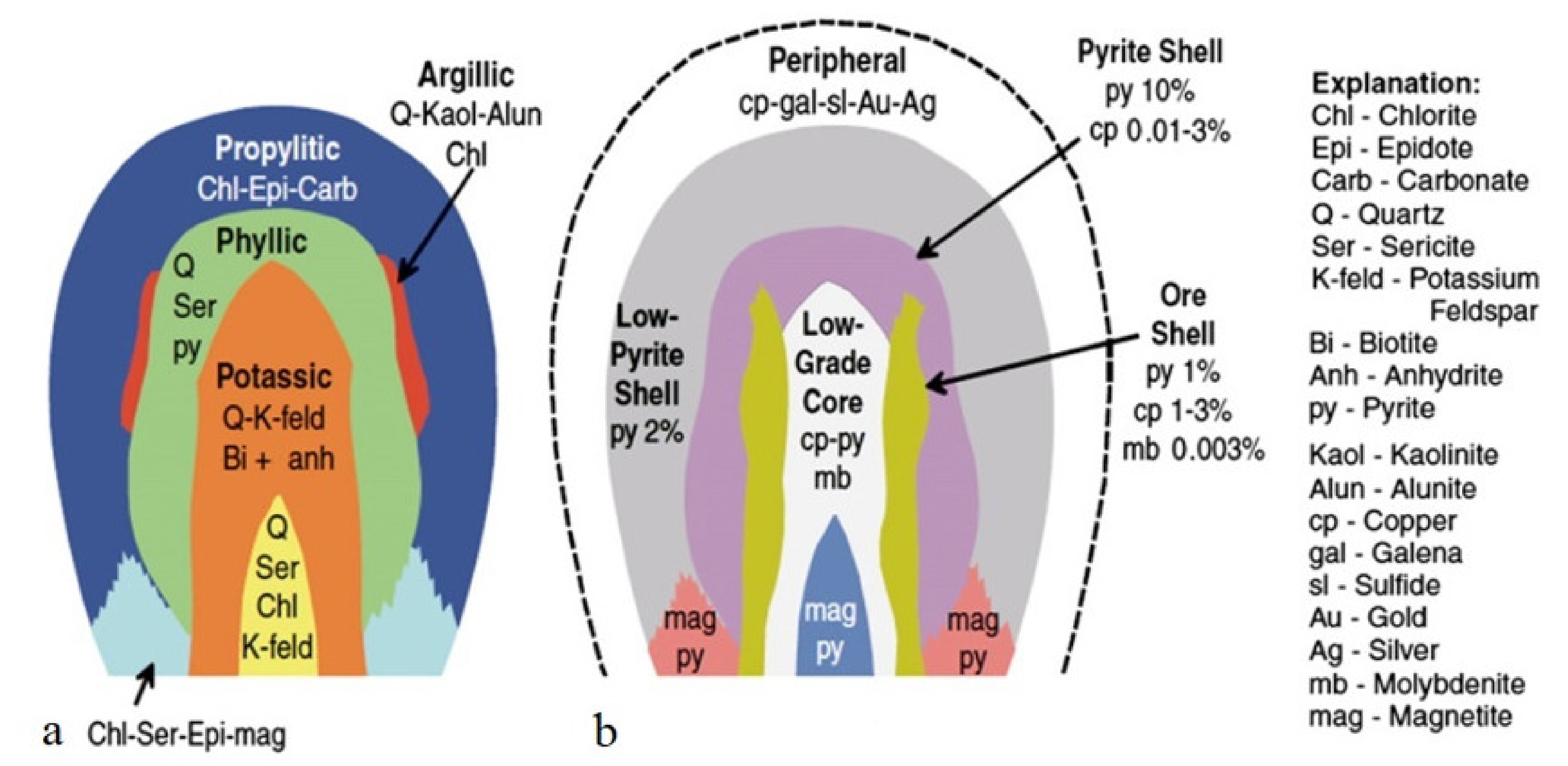
  90. Lowell, J.D.; Guilbert, J.M. Lateral and vertical alteration-mineralization zoning in porphyry ore deposits. Econ. Geol. 1970, 65, 373–408. [Google Scholar] [CrossRef]
  91. John, D.A.; Ayuso, R.A.; Barton, M.D.; Blakely, R.J.; Bodnar, R.J.; Dilles, J.H.; Gray, F.; Graybeal, F.T.; Mars, J.C.; McPhee, D.K.; et al. Porphyry Copper Deposit Model: Chapter B of Mineral Deposit Models for Resource Assessment; U.S. Geological Survey Science Investigation Report, 2010-5070-B; U.S. Geological Survey: Reston, VA, USA, 2010; p. 169.
  92. Hollister, V.F. An appraisal of the nature and source of porphyry copper deposits. Miner. Sci. Eng. 1975, 7, 225–233. [Google Scholar]
  93. Hutchison, C.S. Economic Deposits and Their Tectonic Setting; Macmillan Higher Education: London, UK, 1983. [Google Scholar]
  94. Evans, A.M. Ore Geology and Industrial Minerals: An Introduction; Blackwell Science Publications: Hoboken, NJ, USA, 1993. [Google Scholar]
  95. Rowan, L.C.; Goetz, A.F.H.; Ashley, R.P. Discrimination of hydrothermally altered and unaltered rocks in visible and near infrared multispectral images. Geophysics 1977, 42, 522–535. [Google Scholar] [CrossRef]
  96. Jun, L.; Songwei, C.; Duanyou, L.; Bin, W.; Shuo, L.; Liming, Z. Research on false color image composite and enhancement methods based on ratio images. Int. Arch. Photogramm. Remote Sens. Spat. Inf. Sci. 2008, 37, 1151–1154. [Google Scholar]
  97. Mars, J.C.; Rowan, L.C. Regional mapping of phyllic- and argillic-altered rocks in the Zagros magmatic arc, Iran, using advanced spaceborne thermal emission and reflection radiometer (ASTER) data and logical operator algorithms. Geosphere 2006, 2, 161–186. [Google Scholar] [CrossRef]
  98. Mars, J.C. Hydrothermal Alteration Maps of the Central and Southern Basin and Range Province of the United States Compiled from Advanced Spaceborne Thermal Emission and Reflection Radiometer (ASTER) Data; U.S. Geological Survey, Open-File Report 2013–1139; U.S. Geological Survey: Reston, VA, USA, 2013; p. 5.
  99. Altman, N.S. An introduction to kernel and nearest-neighbor nonparametric regression. Am. Stat. 1992, 46, 175–185. [Google Scholar]
  100. Devroye, L.; Gyorfi, L.; Krzyzak, A.; Lugosi, G. On the strong universal consistency of nearest neighbor regression function estimates. Ann. Stat. 1994, 22, 1371–1385. [Google Scholar] [CrossRef]
  101. Mitchell, T.M. Machine Learning; McGraw-Hill Education: Burr Ridge, IL, USA, 1997. [Google Scholar]
  102. Abedi, M.; Norouzi, G.H. Integration of various geophysical data with geological and geochemical data to determine additional drilling for copper exploration. J. Appl. Geophys. 2012, 83, 35–45. [Google Scholar] [CrossRef]
  103. Zaremotlagh, S.; Hezarkhani, A.; Sadeghi, M. Detecting homogenous clusters using whole-rock chemical compositions and REE patterns: A graph-based geochemical approach. J. Geochem. Explor. 2016, 170, 94–106. [Google Scholar] [CrossRef]
  104. Ghannadpour, S.S.; Hezarkhani, A.; Roodpeyma, T. Combination of separation methods and data mining techniques for prediction of anomalous areas in Susanvar, Central Iran. J. Afr. Earth Sci. 2017, 134, 516–525. [Google Scholar] [CrossRef]
  105. Golmohammadi, A.; Jafarpour, B. Reducing uncertainty in conceptual prior models of complex geologic systems via integration of flow response data. Comput. Geosci. 2020, 24, 161–180. [Google Scholar] [CrossRef]
  106. Shahabi, H.; Shirzadi, A.; Ghaderi, K.; Omidvar, E.; Al-Ansari, N.; Clague, J.J.; Geertsema, M.; Khosravi, K.; Amini, A.; Bahrami, S.; et al. Flood detection and susceptibility mapping using Sentinel-1 Remote Sensing Data and a Machine Learning Approach: Hybrid intelligence of bagging ensemble based on k-nearest neighbor classifier. Remote Sens. 2020, 12, 266. [Google Scholar] [CrossRef] [Green Version]
  107. Cover, T.; Hart, P. Nearest neighbor pattern classification. IEEE Trans. Inf. Theory 1967, 13, 21–27. [Google Scholar] [CrossRef]
  108. Devroye, L. On the asymptotic probability of error in nonparametric discrimination. Ann. Stat. 1981, 9, 1320–1327. [Google Scholar] [CrossRef]
  109. Kumar, Y.; Janardan, R.; Gupta, P. Efficient algorithms for reverse proximity query problems. In Proceedings of the 16th ACM SIGSPATIAL International Conference on Advances in Geographic Information Systems, Irvine, CA, USA, 5–7 November 2008; Association for Computing Machinery: New York, NY, USA; pp. 1–10.
  110. Ramamohanarao, K.; Fan, H. Patterns based classifiers. World Wide Web 2007, 10, 71–83. [Google Scholar] [CrossRef]
  111. Aggarwal, C.C.; Hinneburg, A.; Keim, D.A. On the surprising behavior of distance metrics in high dimensional space. In Proceedings of the International Conference on Database Theory; Springer: Berlin/Heidelberg, Germany, 2001; pp. 420–434. [Google Scholar]
  112. Sabins, F.F. Remote sensing for mineral exploration. Ore Geol. Rev. 1999, 14, 157–183. [Google Scholar] [CrossRef]
Figure 1. (a) Location of the study area in Troud Range (modified after Reference [54]); (b) lithological map of the study area (modified after Reference [62]).
Minerals 12 00103 g001
Figure 2. Geochemical sampling network in the study area (the false-color composites of Sentinel-2 MSI; band 12 in red, band 8 in green, and band 2 in blue).
Minerals 12 00103 g002
Figure 3. Alteration zones associated with porphyry-Cu deposit (modified after Reference [90]): (a) schematic cross section of alteration zones; (b) schematic cross section of ores associated with each alteration zone.
Minerals 12 00103 g003
Figure 4. Geochemical maps of (a) supra-ore and (b) sub-ore elements, zones I and II, in the study area.
Minerals 12 00103 g004
Figure 5. (a) Vertical geochemical zonality models for porphyry-Cu deposits based on typical standard porphyry-Cu deposits in Kazakhstan, Bulgaria, Armenia, and Iran (modified after Reference [71]); (b) geochemical model for porphyry-Cu deposit based on the porphyry Cu deposits database comprising Aktogy (Kazakhstan), Asarel (Bulgaria), Tekhut (Armenia), and Sungun (Iran) (modified after Reference [2]).
Minerals 12 00103 g005
Figure 6. (a) PC1 image in the study area; (b) eigenvector obtained from PCA of six Sentinel-2 MSI bands (bands 2, 3, 4, 8, 11 and 12).
Minerals 12 00103 g006
Figure 7. Maps of lineaments: (a) zone I and (d) zone II; lineaments density for (b) zone I and (e) zone II; existing faults for (c) zone I and (f) zone II.
Minerals 12 00103 g007
Figure 8. Orientations of lineaments of (a) zone I and (c) zone II compared to the faults of (b) zone I and (d) zone II.
Minerals 12 00103 g008
Figure 9. Band ratios of Sentinel-2 MSI image for identifying ferric iron (band 4/band 3): (a) zone I and (c) zone II; ferrous iron (band 12/band 8) + (band 3/band 4) in (b) zone I and (d) zone II on band 8.
Minerals 12 00103 g009
Figure 10. False-color composites of ASTER (band 4 in red, band 6 in green, and band 8 in blue) in (a) zone II and (b) zone I.
Minerals 12 00103 g010
Figure 11. Hydrothermal alteration obtained from ASTER using logical operator algorithms. (a) Argillic and phyllic alteration in zone I; (b) hydrothermal silica-rich, propylitic alteration (carbonate), and propylitic alteration (epidote-chlorite) in zone I; (c) argillic, phyllic, and propylitic (carbonate) alteration and hydrothermal silica-rich in zone II.
Minerals 12 00103 g011
Figure 12. Geological layer map obtained by combining rock units, faults, and alterations layers by using the KNN algorithm in zone I.
Minerals 12 00103 g012
Table 1. Background, threshold, and Clarke values for supra-ore (Pb and Zn) and sub-ore (Cu and Mo) elements in the study area.
ValuesPb (ppm)Zn (ppm)Cu (ppm)Mo (ppm)
Background 13.56243.30.58
Threshold 19.690.678.10.88
Clarke (Beus and Grigorian, 1977) [12]1275401.1
Table 2. Areal productivity, mineralization coefficient, and zonality index introduced by Solovov and zonality index introduced by Grigorian for Cu, Mo, Pb, and Zn elements in zones I and II.
ZoneElementsP, m2% η ( α ) K S K G
Zone ICu1,430,818,85119.620.180.71
Mo6,626,0210.0735
Pb12,649,6760.3564
Zn133,323,5642.856
Zone IICu1,094,297,3258.626.5728.23
Mo32,266,7120.275
Pb552,971,5294.2
Zn1,696,662,82516
Table 3. The logical operator algorithms used with ASTER to map hydrothermally altered rocks in zones I and II (modified after Reference [98]). (b: band; float: floating point; le: less than or equal to; lt: less than; ge: greater than or equal to; gt: greater than.)
ZoneHydrothermal AlterationAlgorithm
Zone IHydrothermal silica-rich (hydrous silica, chalcedony, opal)
Propylitic (carbonate)
Propylitic (epidote–chlorite)
Argillic (alunite, kaolinite)
Phyllic (sericite–muscovite)
((float(b3)/b2) le 1.06) and ((float(b4)/b7) ge 1.06) and ((float(b13)/b12) ge 1.016) and ((float(b12)/b11) lt 1.08)
((float(b3)/b2) le 1.06) and ((float(b6)/b8) gt 1.04) and (b5 gt b6) and (b7 gt b8) and (b9 gt b8) and ((float(b13)/b14) gt 1.005)
((float(b3)/b2) le 1.06) and ((float(b6)/b8) gt 1.04) and ((float(b5)/(float(b4)/b6)) gt 0.513) and (b5 gt b6) and (b6 gt b7) and (b7 gt b8) and (b9 gt b8) and ((float(b13)/b14) le 1.005)
((float(b3)/b2) le 1.06) and ((float(b4)/b6) gt 1.06) and ((float(b5)/b6) le 1.04) and ((float(b7)/b6) ge 1.04)
((float(b3)/b2) le 1.06) and ((float(b4)/b6) gt 1.06) and ((float(b5)/b6) gt 1.04) and ((float(b7)/b6) ge 1.04)
Zone IIHydrothermal silica-rich (hydrous silica, chalcedony, opal)
Propylitic (carbonate)
Propylitic (epidote–chlorite)
Argillic (alunite, kaolinite)
Phyllic (sericite–muscovite)
((float(b3)/b2) le 0.66) and ((float(b4)/b7) ge 1.03) and ((float(b13)/b12) ge 1.156) and ((float(b12)/b11) lt 1.065)
((float(b3)/b2) le 0.66) and ((float(b6)/b8) gt 1.066) and (b5 gt b6) and (b7 gt b8) and (b9 gt b8) and ((float(b13)/b14) gt 0.91)
((float(b3)/b2) le 0.66) and ((float(b6)/b8) gt 1.066) and ((float(b5)/(float(b4)/b6)) gt 0.5) and (b5 gt b6) and (b6 gt b7) and (b7 gt b8) and (b9 gt b8) and ((float(b13)/b14) le 0.91)
((float(b3)/b2) le 0.66) and ((float(b4)/b6) gt 0.97) and ((float(b5)/b6) le 1.04) and ((float(b7)/b6) ge 1.04)
((float(b3)/b2) le 0.66) and ((float(b4)/b6) gt 0.97) and ((float(b5)/b6) gt 1.04) and ((float(b7)/b6) ge 1.04)
Publisher’s Note: MDPI stays neutral with regard to jurisdictional claims in published maps and institutional affiliations.

