Study on the Improved Method for Calculating Traveltime and Raypath of Multistage Fast Marching Method

Abstract

The traditional Fast Marching Method (FMM) based on the finite-difference scheme can solve the traveltime of first arrivals; however, the accuracy and efficiency of FMM are usually affected by the finite-difference schemes and grid size. The Vidale finite-difference scheme and double-grid technology are adopted to replace the traditional first-order and second-order finite-difference schemes in this paper to improve the computation accuracy and efficiency. The traditional FMM does not provide the corresponding raypath calculation methods, and in view of the interoperability of FMM and the linear travel time interpolation (LTI) method, we introduce the linear interpolation method into FMM ray tracing to compute the raypath and take into consideration the secondary source located inside the grid cell to improve the accuracy and stability of the raypath calculation. With these measures and the application of the multistage approach, we successfully completed the improved Multistage FMM (MFMM) ray tracing, which can track first arrivals and any type of primary and multiple reflection waves. Through the theoretical and actual field model tests, the computation accuracy and efficiency of the improved MFMM are proven to be higher than that under traditional first-order and second-order finite-difference schemes, the correctness and effectiveness of the interpolation method for raypath calculation are verified, and the improved MFMM has demonstrated good adaptability and stability for complex models. The improvements for the MFMM in this paper are successfully applied in two-dimensional cases and need to be extended to three-dimensional situations.

1. Introduction

Ray tracing is widely used in various fields of seismic exploration, providing an effective means for pre-stack migration, velocity analysis, and tomography. With the successful application of Kirchhoff integral pre-stack depth migration in complex structure imaging, many grid-based ray tracing methods are developed rapidly, and the finite-difference ray tracing method [1,2] is one of the most representative algorithms.

Vidale [1] uses the finite-difference method to solve the eikonal equation and computes the traveltime by the box expansion method, but it always loses stability in the media with drastic changes in velocity, and the box expansion process does not conform to the law of wavefront propagation. Several scholars have improved this method [3,4,5]. Based on the upwind finite-difference scheme, Sethian [6] first proposes the Fast Marching Method (FMM) to compute the first arrivals traveltime, and the wavefront expansion conforms to the propagation law of seismic wave, then Sethian [7] and Popovici [8] improve this method. FMM has the advantages of high precision, high efficiency, good flexibility, and unconditional stability [6]. Rawlinson and Sambridge [9,10] propose the multistage approach to realize the multi-seismic phase tracing of Multistage FMM (MFMM) and point out that the second-order finite-difference scheme can ensure the computation accuracy and efficiency of the traveltime to a certain extent; meanwhile, using the refined grids near the seismic source can also improve the traveltime computation accuracy. In particular, the proposed Multi-Stencils FMM (MSFM) [11] significantly improves the computation accuracy of FMM. Several scholars have presented improved methods for higher accuracy and efficiency [12,13,14,15], which have been proven to be effective for the first arrivals traveltime computation.

When using the finite-difference method to compute the global-discrete traveltime field, if the ray directions are computed at the same time, it is necessary to compute the ray vectors of all grid nodes and all possible directions [16,17], which increases the storage space, reduces the computation accuracy and efficiency due to the secondary source can only be located on grid node and boundary [18,19]. It is common to track the raypath in reverse by computing the maximum gradient direction of the computed traveltime field [9,10,20,21], but the computation details are not given in these papers. To complete FMM raypath calculation, Rawlinson et al. propose the raylet method, and the multi-valued raypath of the source and the receiving points can be obtained by computing the derivative of the total traveltime from the given point to the source and the receiving points [22]; Wei et al. add the inverse interpolation method to improve the computation accuracy of the secondary source points [23]. Wang et al. track the raypath of FMM by computing the steepest descent direction of the traveltime gradient [24]. Since the linear traveltime interpolation (LTI) method [25] and the steepest descent method [24] only consider the traveltime and raypath of the secondary source located on the grid node and boundary, theydo not deal with the case when the secondary source is inside the grid cell. The raypath may be zigzagged or merged incorrectly with adjacent raypath when dealing with the transparent reflection interface, which reduces the computation accuracy of raypath [18,19,26]. To solve these problems, the interpolation method is usually used to compute the traveltime and traveltime gradient of any point in the model area. Zhang Dong et al. propose Maximum Traveltime Gradient Ray Tracing (MTG) based on cubic B-spline interpolation, which can compute the traveltime gradient at any point in the model region [18,19]. However, it is not suitable for media with drastic changes in velocity. Then the linear interpolation method [25], the Chebyshev interpolation method [27] and the model parameterization [28] are used to solve this problem. Zhang Yun et al. complete multi-seismic phase tracking of MFMM by computing the traveltime gradient [29].

In this paper, we adopt the Vidale finite-difference [1,30] and double-grid technology [5,6] to improve the computation accuracy and efficiency of the traveltime. Then the linear interpolation method is used to track the raypath, especially considering the secondary source appears inside the grid cell, completing the traveltime and raypath computation of improved MFMM. The correctness and effectiveness of the improvements in this paper are verified by numerical simulation of the typical models and the Marmousi model. We also test the improved MFMM by the velocity model of Xiong’an New Area in China [31,32]. The results can describe the first break and reflection events well. Our research in this paper improves the numerical simulation of seismic ray tracing and provides a basis for further studies on seismic data processing and denoising, seismic image analysis, seismic tomography and inversion [33,34,35].

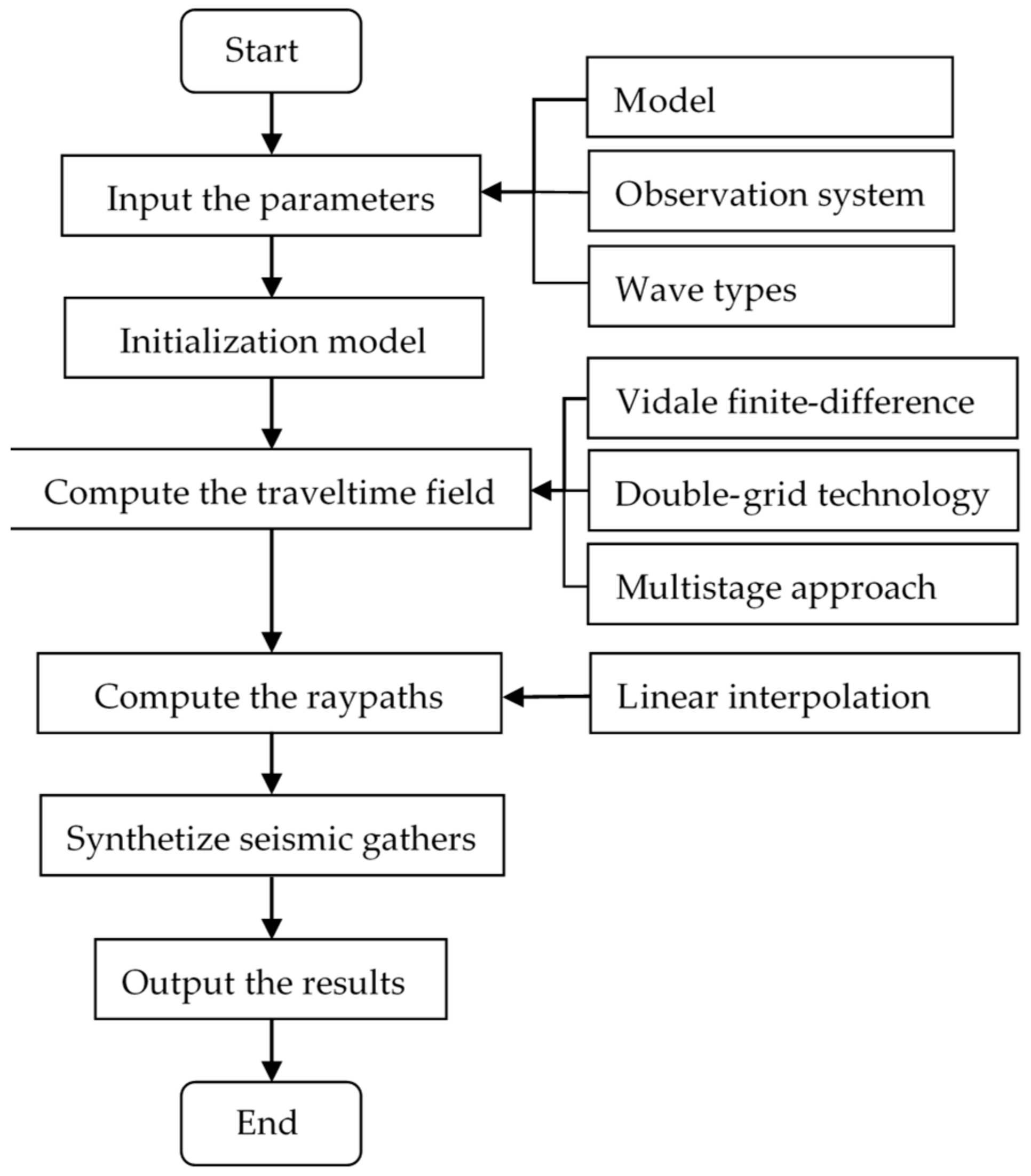
2. Calculation Method of Traveltime

2.1. Finite-Difference Scheme

The two-dimensional eikonal equation is:

$${\left[\frac{\partial t\left(x,z\right)}{\partial x}\right]}^2+{\left[\frac{\partial t\left(x,z\right)}{\partial z}\right]}^2=s^2\left(x,z\right)$$

(1)

where t is the traveltime of the seismic wave, and s is the slowness of the seismic wave. The traditional FMM uses the upwind finite-difference method to solve the eikonal equation to obtain the first arrivals traveltime [6]. In this paper, the traditional and improved Vidale finite-difference [1,30] schemes are used to discrete the eikonal equation.

Figure 1 shows the three types of the Vidale finite-difference schemes, and the traveltime can be obtained by solving Equation (1), so the expression of t_c in Figure 1a is as follows:

$$t_c=\min \left[t_a+\sqrt{2{\left(\overline{s}h\right)}^2-{\left(t_d-t_b\right)}^2},t_a+\sqrt{2}sh,t_b+sh,t_d+sh\right]$$

(2)

The expression of t_c in Figure 1b is:

$$t_c=\min \left[t_a+\sqrt{{\left(\overline{s}h\right)}^2-\frac{1}{4}{\left(t_d-t_b\right)}^2},t_a+sh,t_b+\sqrt{2}sh,t_d+\sqrt{2}sh\right]$$

(3)

The improved expression of t_c in Figure 1c is:

$$t_c=\min \left[t_a+\max \left[\frac{\overline{s}h}{\sqrt{2}},\sqrt{{\left(\overline{s}h\right)}^2-{\left(t_b-t_a\right)}^2}\right],t_a+sh,t_b+\sqrt{2}sh\right]$$

(4)

where is the average slowness of all grid nodes in each equation. By using Equations (2)–(4), the traveltime of the whole model area can be computed through the narrow-band expansion of FMM [6].

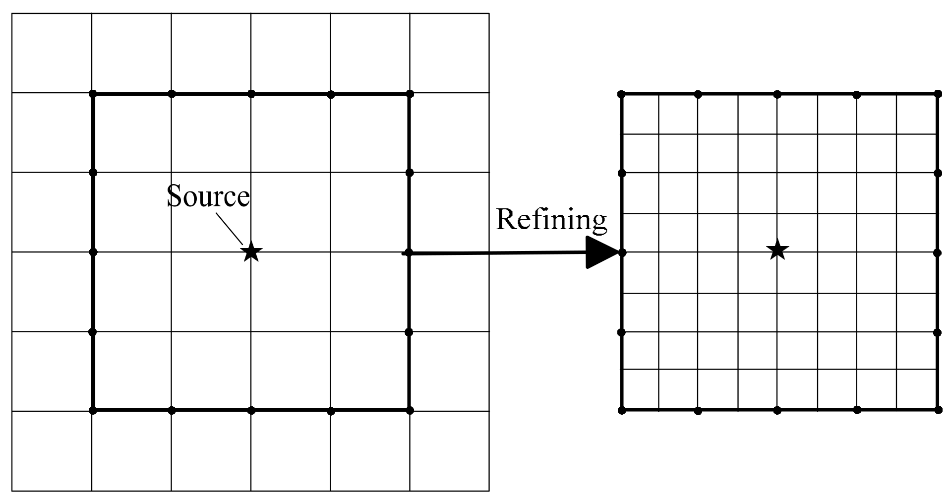
2.2. Double-Grid Technology

The FMM computation errors of traveltime are mainly concentrated near the source. Rawlinson and Sambridge [9,10] refine the grids near the source to improve this problem. In the same way, the double-grid technology is used in this paper to refine the original grids near the source to achieve a similar effect, as shown in Figure 2.

The processes of double-grid technology are as follows: refine the grids near the source, compute the traveltime on all grid nodes of this area by improved FMM, and then return the high-precision traveltime to the original grid node. In this process, two parameters, the number of expanded grid layers around the source and the number of refined points of each grid, determine the computation accuracy and efficiency, while the computation efficiency will decrease with the increase of refined grids. Since the traveltime errors of FMM mainly surround the source, the preferred way is to use fewer expanded grid layers and more refined points of each grid. In practical application, the appropriate parameters can be set through efficiency and error analysis.

3. Calculation Method of Raypath

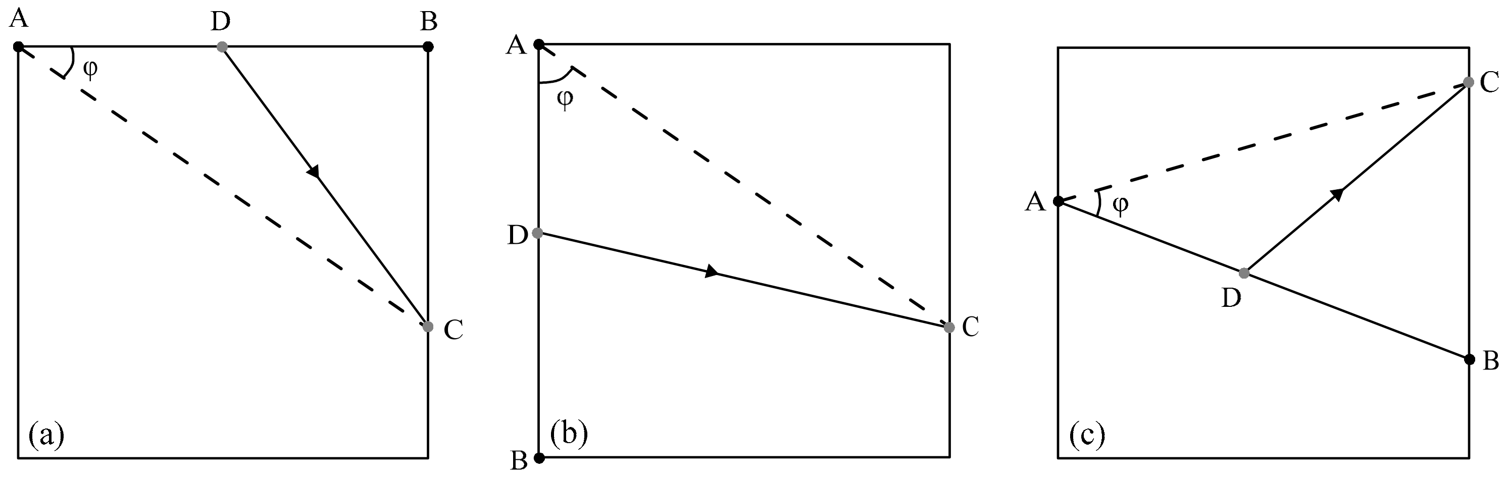
3.1. The Linear Interpolation Method

After obtaining the traveltime field of the model area, the linear interpolation method [25] is adopted to compute the raypath. As shown in Figure 3, in the model area with the rectangular grids, points A and B are the known points, the coordinates are (x_a, z_a) and (x_b, z_b), the traveltimes are t_a and t_b, respectively, and point C and point D are the secondary sources need to be solved, the ray is from point D to point C. So the raypath can be computed by the coordinates of the secondary source D (x_d, z_d) and traveltime of point C t_c.

Based on the linear hypothesis, the traveltime of point D t_d can be obtained by linear interpolation with t_a and t_b, i.e.,

$$t_d=t_a+\left(t_b-t_a\right)r/\left|AB\right|$$

(5)

where point A is the minimum traveltime point, satisfying t_a ≤ t_b; r is the distance between point A and point D, satisfying 0 ≤ r ≤ |AB|, and |AB| is the distance between point A and point B. Since the ray at point C comes from point D, t_c can be expressed as:

$$t_c=t_d+\left|CD\right|/v=t_d+\sqrt{r^2+{\left|AC\right|}^2-2r\left|AC\right|\cos \phi }/v$$

(6)

where v is the wave velocity, φ is the angle between lines AB and AC, |CD| and |AC| represent the distances between corresponding points. Taking Equation (5) into Equation (6):

$$t_c=t_a+\left(t_b-t_a\right)r/\left|AB\right|+\sqrt{r^2+{\left|AC\right|}^2-2r\left|AC\right|\cos \phi }/v$$

(7)

As can be seen from Equation (7), t_c is a function about r. According to Fermat’s principle, the traveltime of the ray from point D to point C is the smallest, and its traveltime gradient is zero; that is:

$$\partial t_c/\partial r=0$$

(8)

Taking Equation (7) into Equation (8):

$$\left(t_b-t_a\right)/\left|AB\right|+\left(r-\left|AC\right|\cos \phi \right)/\sqrt{r^2+{\left|AC\right|}^2-2r\left|AC\right|\cos \phi }/v=0$$

(9)

r can be obtained by solving Equation (9):

$$r=\left|AC\right|\left[\cos \phi -\frac{\left(t_b-t_a\right)\sin \phi }{\sqrt{{\left|AB\right|}^2/v^2-{\left(t_b-t_a\right)}^2}}\right]$$

(10)

Then the coordinates of point D can be obtained:

$$\{\begin{array}{l}{x}_d=x_a+\left(x_b-x_a\right)r/\left|AB\right|\\ z_d=z_a+\left(z_b-z_a\right)r/\left|AB\right|\end{array}$$

(11)

Meanwhile, taking Equation (10) into Equation (7), we can obtain t_c:

$$t_c=t_a+\frac{\left|AC\right|}{\left|AB\right|}\left[\cos \phi \left(t_b-t_a\right)+\sin \phi \sqrt{\frac{{\left|AB\right|}^2}{v^2}-{\left(t_b-t_a\right)}^2}\right]$$

(12)

Equations (10)–(12) are suitable for traveltime computation with arbitrary shapes.

The rectangular grid is used to discretize the model area in this paper. When point A and point B are located on the grid nodes, Equations (10)–(12) can be further simplified. As shown in Figure 3a, when points A, B and D are located on the horizontal boundary of the grid, z_a = z_b, the corresponding equations are:

$$r=\left(x_c-x_a\right)-\frac{\left(t_b-t_a\right)\left(z_c-z_a\right)}{\sqrt{{\left|AB\right|}^2/v^2-{\left(t_b-t_a\right)}^2}}$$

(13)

$$\{\begin{array}{l}{x}_d=x_a+\left(x_b-x_a\right)r/\left|AB\right|\\ z_d=z_a\end{array}$$

(14)

$$t_c=t_a+\frac{1}{\left|AB\right|}\left[\left(x_c-x_a\right)\left(t_b-t_a\right)+\left(z_c-z_a\right)\sqrt{\frac{{\left|AB\right|}^2}{v^2}-{\left(t_b-t_a\right)}^2}\right]$$

(15)

As shown in Figure 3b, when points A, B and D are located on the vertical boundary of the grid, x_a = x_b, the corresponding equations are:

$$r=\left(z_c-z_a\right)-\frac{\left(t_b-t_a\right)\left(x_c-x_a\right)}{\sqrt{{\left|AB\right|}^2/v^2-{\left(t_b-t_a\right)}^2}}$$

(16)

$$\{\begin{array}{l}{x}_d=x_a\\ z_d=z_a+\left(z_b-z_a\right)r/\left|AB\right|\end{array}$$

(17)

$$t_c=t_a+\frac{1}{\left|AB\right|}\left[\left(z_c-z_a\right)\left(t_b-t_a\right)+\left(x_c-x_a\right)\sqrt{\frac{{\left|AB\right|}^2}{v^2}-{\left(t_b-t_a\right)}^2}\right]$$

(18)

In addition to the case of the secondary source D being located on the grid node or boundary, we also have considered the case of the secondary source D being located inside the grid cell, i.e., point A and point B are located at the transparent reflection interface, as shown in Figure 3c, and we use Equations (10)–(12) for the traveltime and raypath computation. Therefore, according to the known conditions of points A-D in Figure 3, the coordinate and traveltime of the secondary source at any location in the model area can be solved by using Equations (10)–(18), which can improve the FMM raypath calculation accuracy.

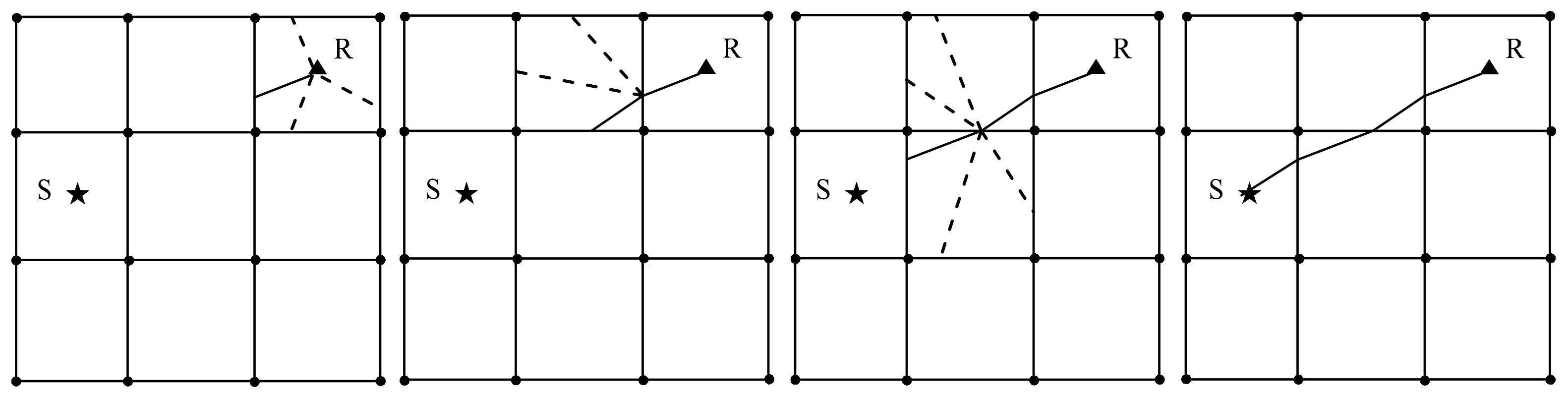
3.2. Raypath Tracing Process

After obtaining the traveltime of all grid nodes, the raypath tracing processes [25] retrieved from the receiving point to the source are shown in Figure 4 and can be summarized into three steps:

(1) Retrieve the coordinates and traveltime of all nodes in the grid where the receiving point is located. If the receiving point is on the grid node, its traveltime can be used directly; if the receiving point is not on the grid node, its traveltime can be computed through linear interpolation by Equation (15) or (18).

(2) Compute the traveltime of all the possible raypath from the boundary of the grid where the receiving point is located by Equation (15) or (18), then select the minimum traveltime raypath and compute the location of the secondary source on this raypath by Equation (14) or (17); if there are transparent reflection interfaces in the grid cell, the secondary source will appear inside the grid cell, and its location can be computed by Equations (10)–(12).

(3) Repeat steps (1) to (2) until the last secondary source reaches the grid where the source is located, then connect the source, all the secondary sources and the receiving points in turn to obtain the whole raypath.

4. Model Test

We use several typical models to test the computation accuracy, efficiency, stability and adaptability of complex models with the interpolation raypath method.

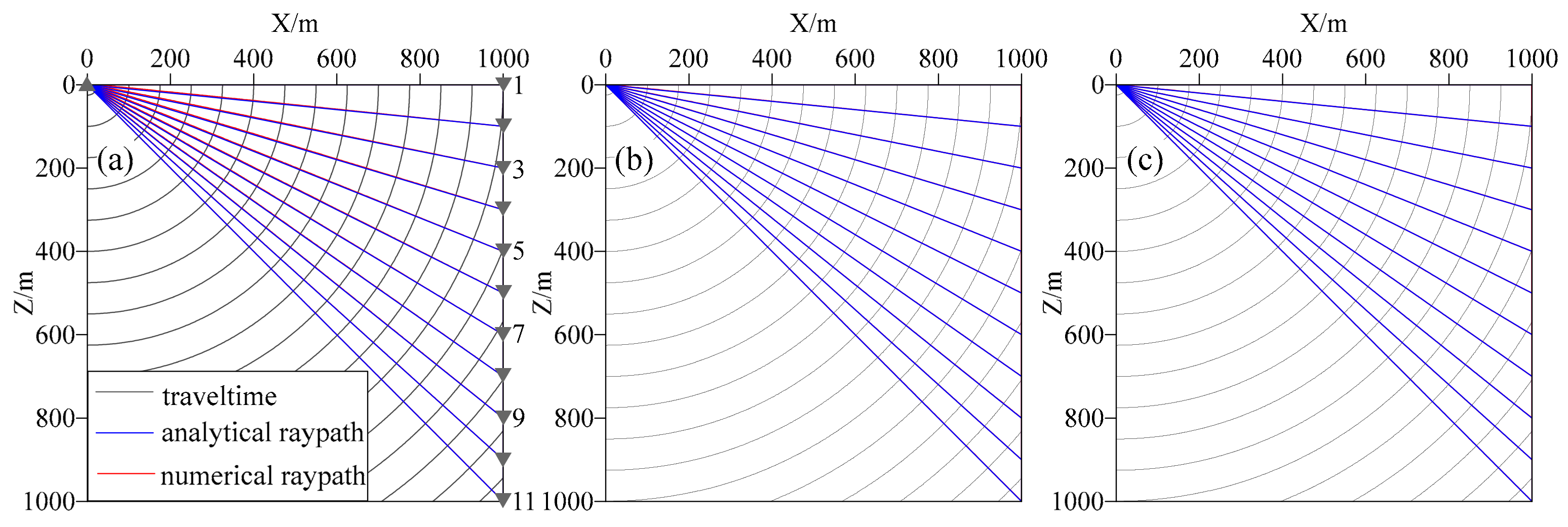
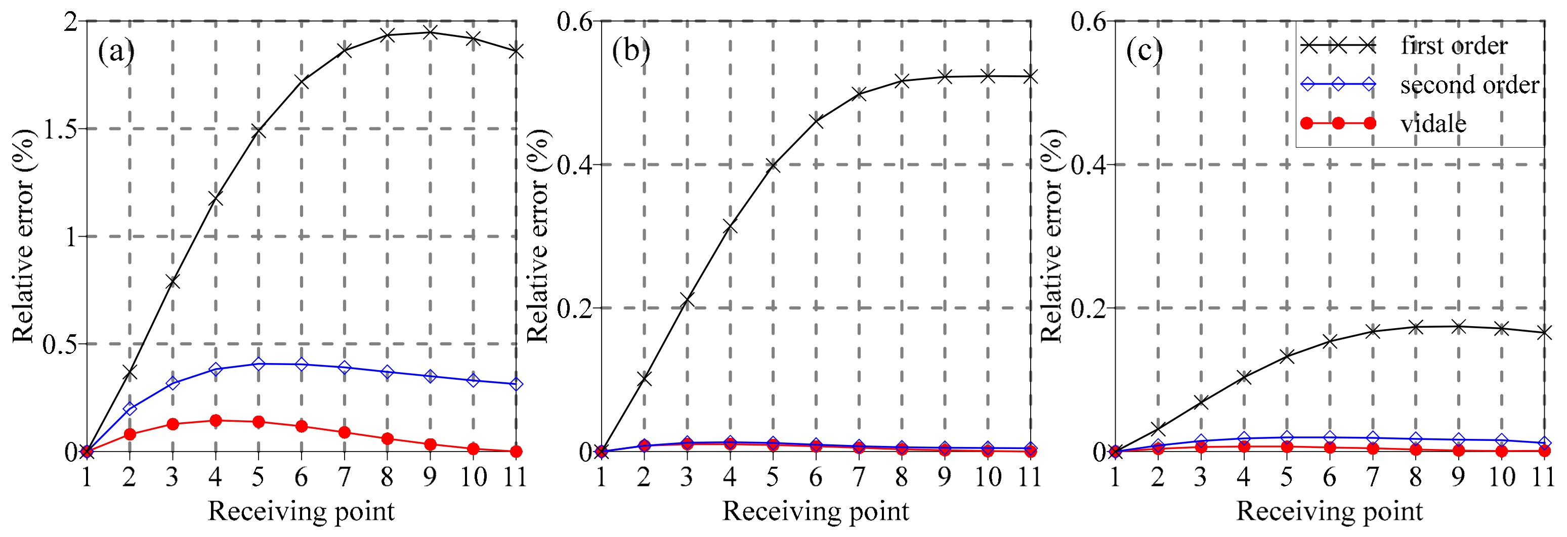
4.1. Homogeneous Model

To analyze the computation accuracy and efficiency of FMM, we design a homogeneous model for forward simulation, with an area of 1000 m × 1000 m and a wave velocity of 1000 m/s. The observation system is shown in Figure 5a. ▲ represents the source. The coordinates are (0, 0) m. ▼ represents the receiving points, which are sequentially arranged on the right boundary of the model, with a channel spacing of 100 m, and there are 11 receiving channels in total. The first-order, second-order and Vidale finite-difference schemes are used with the same grid spacing. The forward modeling results and their comparison are shown in Figure 5 and Figure 6 and

Table 1. CPU time of FMM with different finite-difference schemes and grid spacings.

Finite-Difference Scheme	Grid Spacing
	20 m	20 m (Double-Grid)	1 m
First order	0.1094 s	0.4531 s	2.1250 s
Second order	0.2137 s	1.3437 s	5.8437 s
Vidale	0.1250 s	0.6719 s	3.0156 s

.

It can be seen from Figure 5 that it is feasible to use linear interpolation to compute the raypath of FMM. With the small grid spacing, the numerical raypaths under the first-order, second-order, and Vidale finite-difference schemes are consistent with the analytical raypaths, and the numerical raypaths are orthogonal to the wavefront. Figure 6 shows the relative error between the analytical solution and the numerical solution under different finite-difference schemes. It can be seen from Figure 6a,c that the smaller the grid spacing, the smaller the relative error. From Figure 6a to Figure 6c, we can see the FMM computation accuracy under the Vidale finite-difference scheme is better than that under the first-order and second-order finite-difference schemes. As can be seen from Figure 6b, when the first 20 layers of grids around the source are refined to 1 × 1 m by using the double-grid technology, the computation accuracy under the second-order and the Vidale finite-difference schemes with the grid spacing of 20 m is significantly improved and is equivalent to that with the grid spacing of 1 m. As shown in Table 1, the CPU time of FMM under the Vidale finite-difference scheme is equivalent to that under the first-order finite-difference scheme and also has a higher computation efficiency than that under the second-order finite-difference scheme. The above results show that to obtain the same computation accuracy, the improvements in this paper will take the least CPU time. Therefore, the Vidale finite-difference scheme and double-grid technology can improve the computation accuracy and efficiency of FMM at the same time.

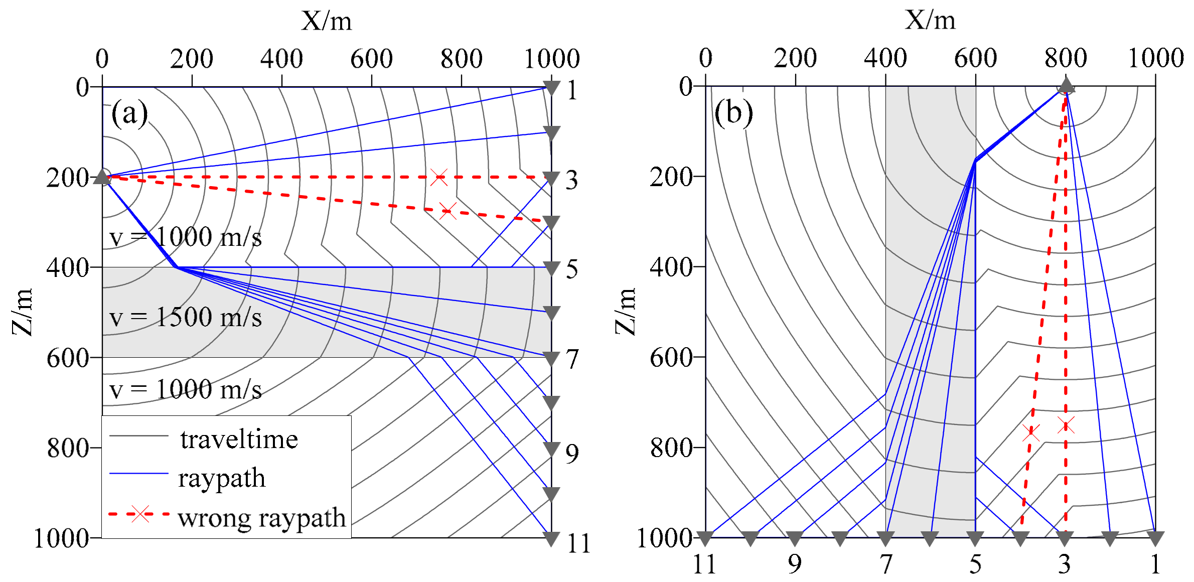
4.2. High-Speed Sandwich Model

To test the correctness of the interpolation method for computing raypaths, we adopt the high-speed sandwich model designed by Asakawa and Kawanaka [25]. The model parameters and observation system are shown in Figure 7. The model area is 1000 × 1000 m. The background wave velocity is 1000 m/s. The wave velocity of the high-speed interlayer is 1500 m/s. Model B is 90° symmetrical with model A. ▲ represents the source. ▼ represents the receiving points. The receiving channel spacing is 100 m, with a total of 11 receiving channels. With the Vidale finite-difference scheme and the same double-grid parameters as Figure 6b, the first arrival waves of FMM ray tracing are shown in Figure 7.

It can be seen from Figure 7 that the first arrivals raypaths obtained by FMM ray tracing are along the normal direction of the wavefront, and the rays received by the third and fourth channels in Figure 7a,b are not directly from the source, but from the refraction of the high-speed layer, which satisfies the Fermat principle and is consistent with the test results of Asakawa and Kawanaka [25], indicating that the numerical raypath we computed is correct. So FMM raypath tracing based on linear interpolation is correct and effective.

4.3. Marmousi Model

We use the Marmousi model to test the adaptability and stability of the interpolation method for complex models and compare the results of FMM and LTI ray tracing. The model area is 3830 × 1210 m, the grid spacing is 10 m and the number of grid nodes is 384 × 122 (Nx × Nz); the source ▲ is located at the bottom interface of the model with coordinates (2790, 1210) m, and the receiving arrangement is located on the top of the model with the receiving channel spacing of 50 m, totaling 77 channels. The forward modeling results and their comparison are shown in Figure 8.

As can be seen from Figure 8a, the FMM wavefront and raypaths can reflect the velocity structure of the Marmousi model correctly. The wavefront in the high-velocity area is faster than that in the low-velocity area. The rays gather in the high-velocity area, bypass the low-velocity area, and scatter at the velocity cusp. The numerical rays always propagate along the minimum traveltime direction, which satisfies the Fermat principle. Comparing Figure 8a with Figure 8b, the wavefront and raypath of FMM and LTI coincide highly with each other. Meanwhile, it can be seen from Figure 8c that the traveltimes of FMM and LTI are highly consistent, and the residual error between them is almost zero. Therefore, FMM ray tracing based on the interpolation method has strong adaptability for complex models, which have been proven to be stable.

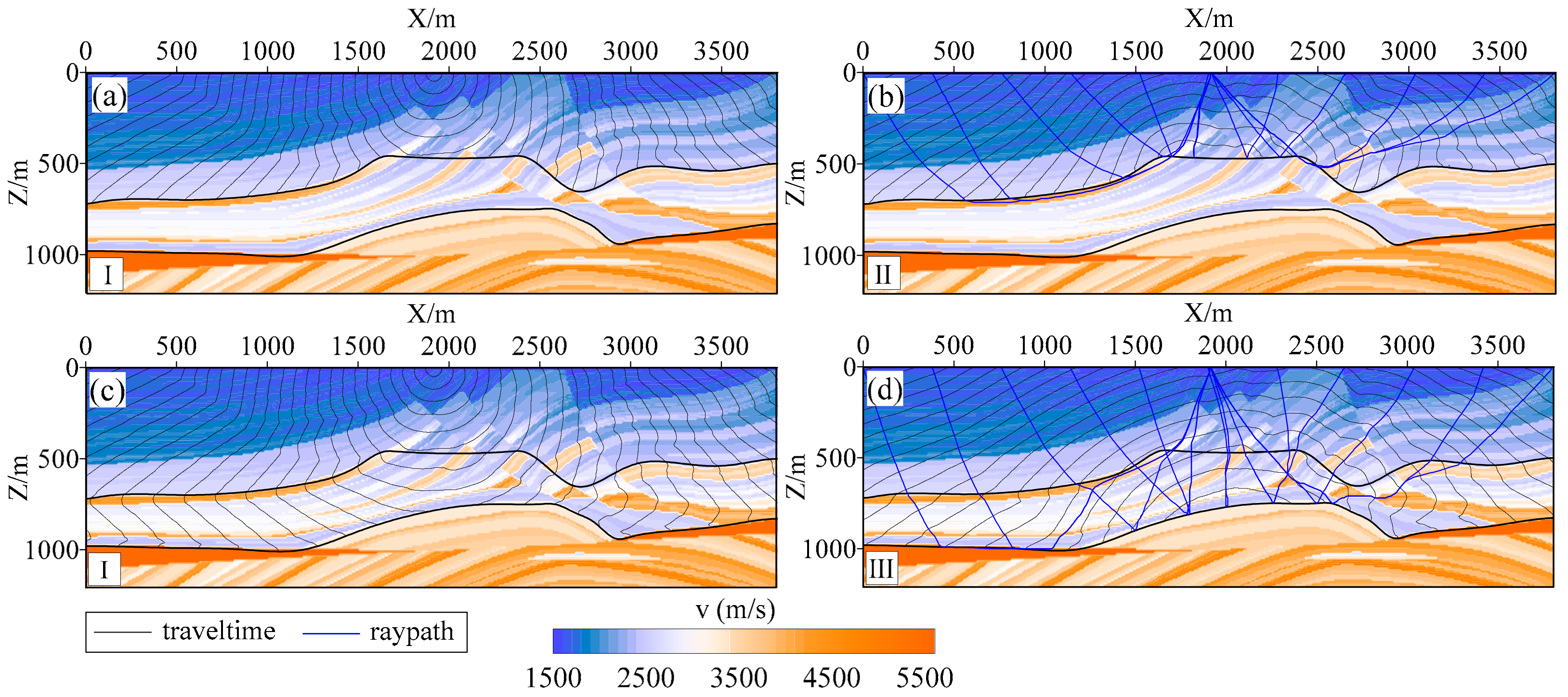
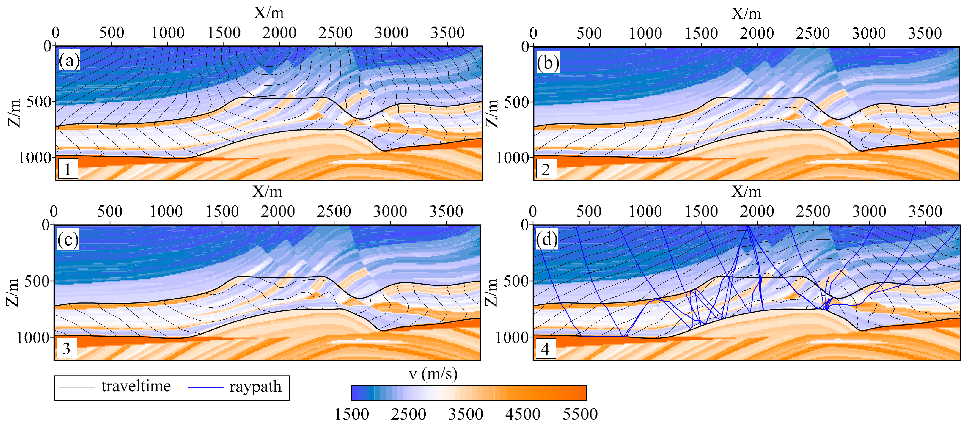
5. MFMM Ray Tracing

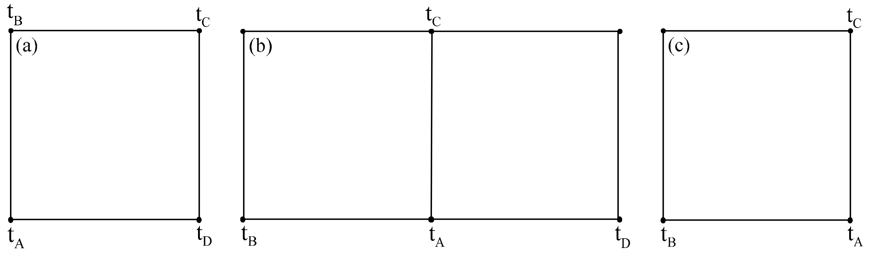
5.1. Multistage Approach

The multistage approach proposed by Rawlinson and Sambridge [9,10] is successfully applied to FMM, which can track the reflected waves and multiple waves. In the process, the computation regions are separated according to the type of waves tracked, and then the traveltime fields are computed in turn, which solves the grid-based multiwave ray tracing problem.

Taking the two-layer velocity model as an example, as shown in Figure 9, the processes of MFMM tracking transmitted and reflected waves are as follows:

(1) Discretize the interface and the velocity model, separate the calculation regions into I and II according to the wave types and compute the wavefront of region I from the source, as shown in Figure 9a;

(2) Compute the wavefront narrowband of the interface; all the nodes of the interface are alive points [6], and their traveltimes cannot be updated, as shown in Figure 9b;

(3) Compute the wavefront of the up-going or down-going waves in each computation region separately from the narrowband in (2), and the processes are as follows:

A. If the waves transmit at the interface, the down-going wavefront in region II can be computed from the narrowband in (2), as shown in Figure 9c;

B. If the waves reflect at the interface, the up-going wavefront in region I can be computed from the narrowband in (2), as shown in Figure 9d;

In this step, if the type of wave tracked from the narrowband in (2) is converted, compute the wavefront of the up-going or down-going waves with the corresponding wave velocity.

(4) Repeat (2) and (3) to compute the wavefront of the transmitted wave, reflected wave and multiple wave.

Figure 10 shows the workflow of the improved MFMM in this paper.

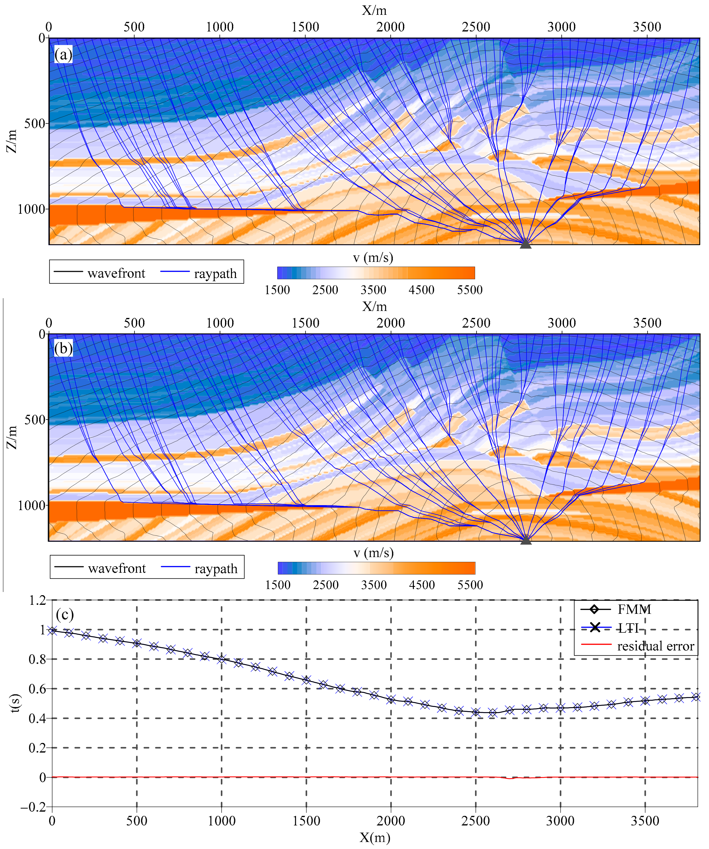
5.2. Marmousi Model Test

We apply the multistage approach [9,10] and linear-interpolation raypath calculation method to FMM and use the Marmousi model to test MFMM. The model parameters are the same as that in Figure 8a. The source ▲ and receiving arrangement ▼ are located at the top interface of the model, with source coordinates (1915, 0) m, and the first receiving channel coordinates (0, 0) m. The receiving channel spacing is 383 m, with 11 receiving channels in total. As shown in Figure 11, two reflection interfaces are given in this model, the computation stages of primary reflection waves are I-II and I-III, and that of multiple reflection waves are 1-2-3-4. The MFMM ray tracing is carried out with the same double grids as in Figure 8a, and the results are shown in Figure 12 and Figure 13. The seismic gathers in Figure 14 describe the first break and reflection events clearly, which are synthesized by Ricker wavelet with a frequency of 30 Hz and a length of 60 ms, and the sampling rate and record length are 1 ms and 1.5 s, respectively.

It can be seen from Figure 12 and Figure 13 that MFMM can track the primary and multiple reflection waves in complex models well, and the wavefront and raypath satisfy the wave propagation law. Meanwhile, the raypath calculation method based on linear interpolation enables MFMM to accomplish all types of wave ray tracing, and it has been proven to have good adaptability and stability for complex models.

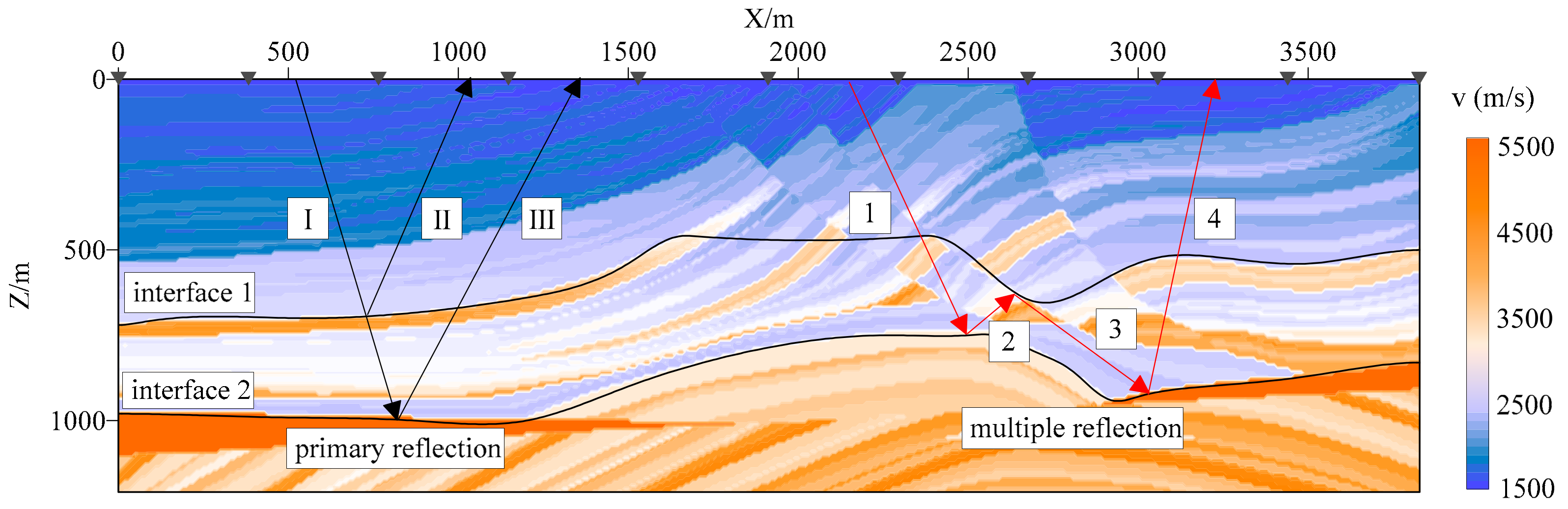
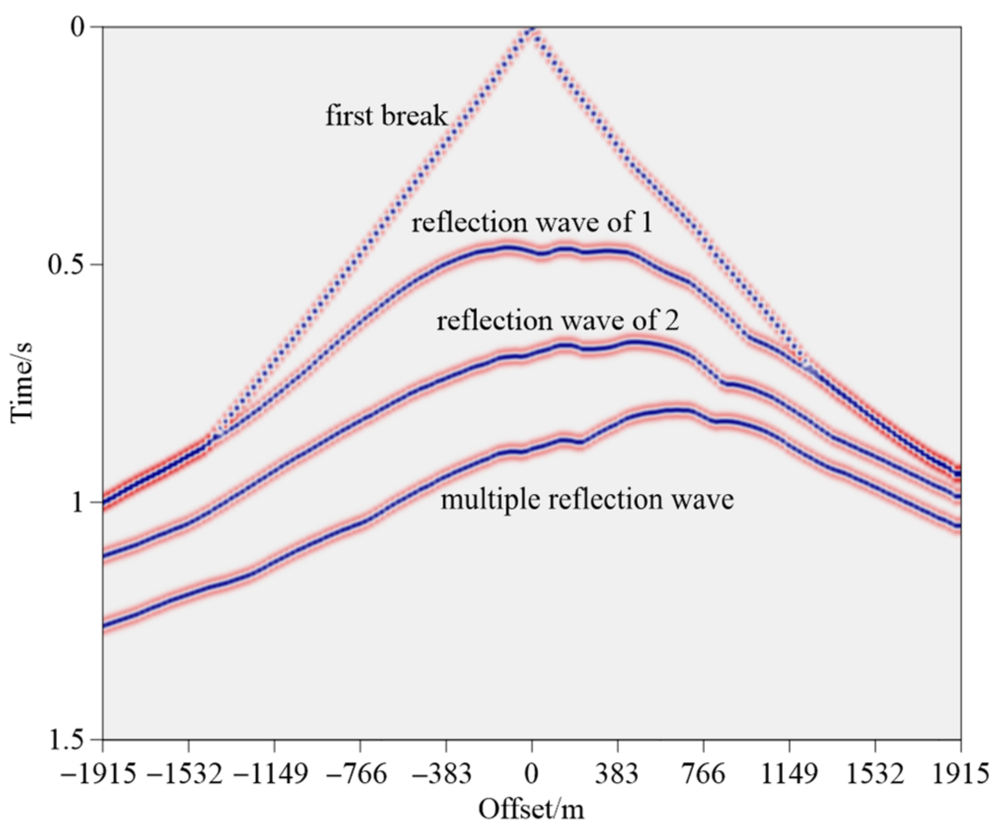
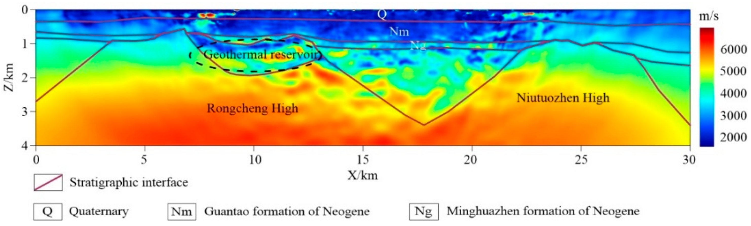
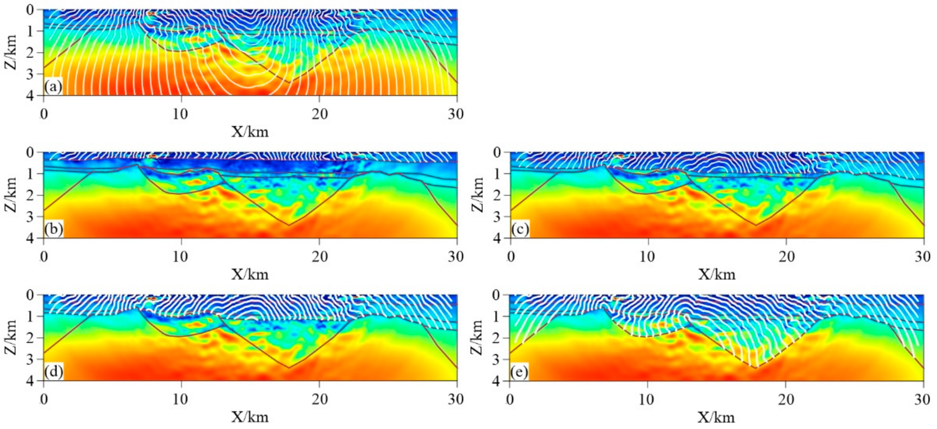
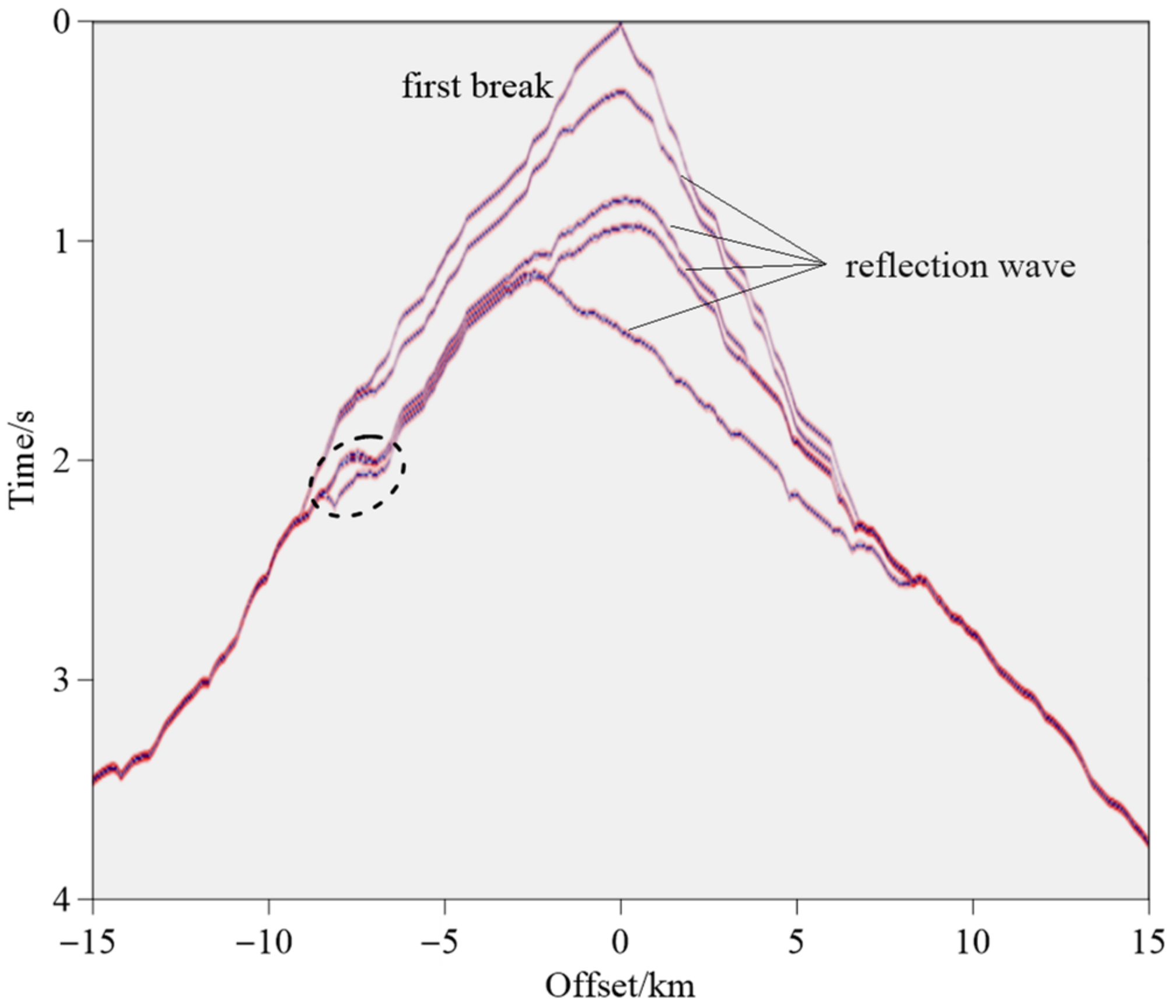
5.3. A Field Example: Xiong’an New Area

Xiong’an New Area is a state-level new area located in Hebei province in China. This area is located in the middle of the Jizhong depression, a part of the eastern block of the North China Craton [37], and it is mainly composed of four structural units: Rongcheng High, the southern Niutuozhen High, the southern Niubei Slope and the Baiyangdian Subsag. The stratigraphy in this area from the top contains Quaternary, Neogene and Paleogene strata. The thickness of the Quaternary (Q) Pingyuan Formation is 348–437 m; the Neogene strata are mainly composed of the Guantao Formation (Ng) with a thickness of 0–424.5 m and the Minghuazhen Formation (Nm) with a thickness of 686–947 m; the bottom of the Paleogene (Pg) strata is regarded as the basement with the shallowest depth of approximately 800 m [38]. China Geology Survey has carried out a two-dimensional seismic survey in this area to make underground structures transparent [31,32], as shown in Figure 15.

Figure 16 shows the velocity model and geological structures of Xiong’an New Area, which is extracted from the interpretation result of seismic profile AA’ in Figure 15; a potential geothermal reservoir is delineated [31]. We can see that this field model is very complex, and the velocity is variable and changes dramatically in some regions. In the numerical simulation, MFMM is carried out to track the first break and the primary reflection waves. The source is located on the surface with x = 15 km, and 1440 receiving channels with a spacing of 20 m are arranged on both sides of the source; the offset is from 10 m to 14,390 m [31].

Figure 17 shows the wavefront of the first break and primary reflection waves of the bottom of Q, the bottom of Nm, the bottom of Ng, the top of Rongcheng High and Niutuozhen High. As can be seen from the results, compared with the low-velocity region, the wavefront is farther and faster in the high-velocity region, which follows the propagation law of seismic waves and can correctly describe the velocity structure of Xiong’an New Area. Benefiting from the multistage approach [9,10], we can obtain the reflection waves of any stratigraphic interface.

We also use the Ricker wavelet with a frequency of 30 Hz and a length of 60 ms to synthesize the seismic gathers, and the sampling rate and record length are 1 ms and 8.0 s, respectively. It can be seen from Figure 18 that the seismic gathers describe the first break and the primary reflection events correctly, and the circle by dotted lines is considered as the reflection gathers of the potential geothermal reservoir. From the above results of the Xiong’an model, the good adaptability and stability of the improved MFMM in this paper are verified once again.

6. Conclusions

In this paper, we adopt the Vidale finite-difference scheme and double-grid technology to improve the computation accuracy and efficiency of traveltime, and the linear interpolation method is used to compute the raypath, considering the case that the secondary source is located inside the grid cell, which improves the computation accuracy of the raypath. The successful application of the multistage approach completes MFMM ray tracing in two-dimensional cases, which can simulate first arrivals and any type of primary and multiple reflection wave ray tracing. Through the forward simulation of typical models, the Marmousi model and the actual model of Xiong’an New Area, the correctness and effectiveness of the improvements in traveltime computation and the interpolation raypath calculation method are verified. The results also show that the improved MFMM in this paper has good adaptability and stability for complex models and provides a reference for the finite-difference ray tracing method, which can be extended to three-dimensional situations.

References

- Vidale, J.E. Finite-difference calculation of traveltimes. Bull. Seismol. Soc. Am. 1988, 78, 2062–2076. [Google Scholar]
- Vidale, J.E. Finite-difference calculations of traveltimes in three dimensions. Geophysics 1990, 55, 521–526. [Google Scholar] [CrossRef] [Green Version]
- Trier, J.V.; Symes, W.W. Upwind finite-difference calculation of traveltimes. Geophysics 1991, 56, 812–821. [Google Scholar] [CrossRef]
- Podvin, P.; Lecomte, I. Finite difference computation of traveltimes in very contrasted velocity model: A massively parallel approach and its associated tools. Geophys. J. R. Astron. Soc. 1991, 105, 271–284. [Google Scholar] [CrossRef] [Green Version]
- Qin, F.H.; Luo, Y.; Olsen, K.B.; Cai, W.Y.; Schuster, G.T. Finite-difference solution of the eikonal equation along expanding wavefronts. Geophysics 1992, 57, 478–487. [Google Scholar] [CrossRef]
- Sethian, J.A. A fast marching level set method for monotonically advancing fronts. Proc. Natl. Acad. Sci. USA 1996, 93, 1591–1595. [Google Scholar] [CrossRef] [Green Version]
- Sethian, J.A.; Popovicit, A.M. 3-D traveltime computation using the fast marching method. Geophysics 1999, 64, 516–523. [Google Scholar] [CrossRef]
- Popovicit, A.M.; Sethian, J.A. 3-D imaging using higher order fast marching traveltimes. Geophysics 2002, 67, 604–609. [Google Scholar] [CrossRef]
- Rawlinson, N.; Sambridge, M. Multiple reflection and transmission phases in complex layered media using a multistage fast marching method. Geophysics 2004, 69, 1338–1350. [Google Scholar] [CrossRef]
- Rawlinson, N.; Sambridge, M. Wave front evolution in strongly heterogeneous layered media using the fast marching method. Geophys. J. Int. 2004, 156, 631–647. [Google Scholar] [CrossRef] [Green Version]
- Hassouna, M.S.; Farag, A.A. Multistencils fast marching methods: A highly accurate solution to the eikonal equation on cartesian domains. IEEE Trans. Pattern Anal. Mach. Intell. 2007, 29, 1563–1574. [Google Scholar] [CrossRef]
- Kim, S. An o(n) level set method for eikonal equations. SIAM J. Sci. Comput. 2001, 22, 2178–2193. [Google Scholar] [CrossRef]
- Danielsson, P.E.; Lin, Q.F. A modified fast marching method. Lect. Notes Comput. Sci. 2003, 2749, 1154–1161. [Google Scholar]
- Yatziv, L.; Alberto, B.; Guillermo, S. O(N) implementation of the fast marching algorithm. J. Comput. Phys. 2005, 212, 393–399. [Google Scholar] [CrossRef] [Green Version]
- Merino-Caviedes, S.; Cordero-Grande, L.; Pérez, M.T.; Casaseca-de-la-Higuera, P.; Martín-Fernández, M.; Deriche, R.; Alberola-López, C. A Second Order Multi-Stencil Fast Marching Method with a Non-Constant Local Cost Model. IEEE Trans. Image Process. 2019, 28, 1967–1979. [Google Scholar] [CrossRef]
- Liu, H.; Meng, F.L.; Li, Y.M. The interface grid method for seeking global minimum travel-time and the correspondent raypath. Chin. J. Geophys. 1995, 38, 823–832. [Google Scholar]
- Zhang, F.X.; Wu, Q.J.; Li, Y.H.; Zhang, R.Q.; Pan, J.T. Application of FMM ray tracing to forward and inverse problems of seismology. Prog. Geophys. 2010, 25, 1197–1205. [Google Scholar]
- Zhang, D.; Zhang, T.T.; Zhang, X.L.; Yang, Y.; Hu, Y.; Qin, Q.Q. A new 3-D ray tracing method based on LTI using successive partitioning of cell interfaces and traveltime gradients. J. Appl. Geophys. 2013, 92, 20–29. [Google Scholar] [CrossRef]
- Zhang, D.; Zhang, T.T.; Qiao, Y.F.; Zhang, Y.; Hu, Y.; Qin, Q.Q. A 3-D ray tracing method based on B-spline traveltime interpolation. Oil Geophys. Prospect. 2013, 48, 559–566. [Google Scholar]
- Serretti, P.; Morelli, A. Seismic rays and traveltime tomography of strongly heterogeneous mantle structure: Application to the Central Mediterranean. Geophys. J. Int. 2011, 187, 1708–1724. [Google Scholar] [CrossRef]
- Li, X.Z.; Zhang, W. Application of Snell’s law in reflection raytracing using the multistage fast marching method. Earthq. Res. Adv. 2021, 1, 41–48. [Google Scholar] [CrossRef]
- Rawlinson, N.; Sambridge, M.; Hauser, J. Multipathing, reciprocal traveltime fields and raylets. Geophys. J. Int. 2010, 181, 1077–1092. [Google Scholar] [CrossRef] [Green Version]
- Wei, P.L.; Sun, J.G.; Meng, X.Y. A ray path calculation method based on grid traveltime. Oil Geophys. Prospect. 2018, 53, 722–729. [Google Scholar]
- Wang, F.; Qu, X.X.; Liu, S.X.; Li, Y.P.; Wu, J.J. A new 3-D ray tracing approach based on both multi-stencils fast marching and the steepest descent. Oil Geophys. Prospect. 2014, 49, 1106–1114. [Google Scholar]
- Asakawa, E.; Kawanaka, T. Seismic ray tracing using linear traveltime interpolation. Geophys. Prospect. 1993, 41, 99–111. [Google Scholar] [CrossRef]
- Zhang, T.T.; Qiu, D.; Zhang, D. A modified 3D traveltime gradient ray tracing method. Oil Geophys. Prospect. 2016, 51, 916–923. [Google Scholar]
- Miao, H.; Sun, J.G.; Wang, R.; Yan, H.Q.; Yi, C.; Wei, L.P. 3D traveltime ray tracing based on Chebyshev polynomials. Oil Geophys. Prospect. 2018, 53, 462–468. [Google Scholar]
- Sun, J.G.; Li, Y.L.; Sun, Z.Q.; Miao, H. Computation of Seismic Traveltimes and Raypath Based on Model Parameterization. J. Jilin Univ. 2018, 48, 343–349. [Google Scholar]
- Zhang, Y.; Yan, X.; Bai, C.Y. Multi-phase seismic ray tracing in 3D undulated layered media based on multistage FMM algorithm. Prog. Geophys. 2018, 33, 1013–1021. [Google Scholar]
- Li, W.J.; Wei, X.C.; Ning, J.R.; Zhang, J.W. A method using improved eikonal equation to compute travel time. Oil Geophys. Prospect. 2008, 43, 589–594. [Google Scholar]
- Wang, K.; Feng, X.; Malcolm, A.; Williams, C.; Wang, X.J.; Zhang, K.; Zhang, B.W.; Yue, H.Y. Multiscale full-waveform inversion with land seismic field data: A case study from the jizhong depression, middle eastern China. Energies 2022, 15, 3223. [Google Scholar] [CrossRef]
- Yue, H.Y.; Wang, K.; Zhang, J.; Liu, J.X.; Wang, X.J.; Zhang, B.W. High-precision imaging technology of deep reflection seismic in Xiong’an New Area and its surroundings. Oil Geophys. Prospect. 2022, 57, 855–869. [Google Scholar]
- Radad, M.; Gholami, A.; Siahkoohi, H.R. A fast method for generating high resolution single-frequency seismic attributes. J. Seism. Explor. 2016, 25, 11–25. [Google Scholar]
- Mafakheri, J.; Kahoo, A.R.; Anvari, R.; Mohammadi, M.; Radad, M.; Monfared, M.S. Expand Dimensional of Seismic Data and Random Noise Attenuation Using Low-Rank Estimation. IEEE J. Sel. Top. Appl. Earth Obs. Remote Sens. 2022, 15, 2773–2781. [Google Scholar] [CrossRef]
- Mousavi, J.; Radad, M.; Soleimani Monfared, M.; Roshandel Kahoo, A. Fault Enhancement in Seismic Images by Introducing a Novel Strategy Integrating Attributes and Image Analysis Techniques. Pure Appl. Geophys. 2022, 179, 1645–1660. [Google Scholar] [CrossRef]
- Ye, P.; Li, Q.C. Improvements of linear traveltime interpolation ray tracing for the accuracy and efficiency. J. Jilin Univ. 2013, 43, 291–298. [Google Scholar]
- Li, S.Z.; Suo, Y.H.; Dai, L.M.; Liu, L.P.; Jiao, Q. Development of the Bohai Bay Basin and destruction of the North China Craton. Earth Sci. Front. 2010, 17, 64–89. [Google Scholar]
- He, D.; Shan, S.; Zhang, Y.; Lu, R.; Zhang, R.; Cui, Y. 3-D geologic architecture of Xiong’an New Area: Constraints from seismic reflection data. Sci. China Earth Sci. 2018, 61, 1007–1022. [Google Scholar] [CrossRef]