Mechanical Behavior Analysis of Fully Grouted Bolts under Axial Cyclic Load

Abstract

Fully grouted bolts are widely used in engineering. In order to deeply understand the load-transfer mechanism of a fully grouted bolt, it is necessary to analyze and study its mechanical behavior under axial cyclic load. First of all, based on the idea of discretization and the force balance analysis of each mass spring element, this study proposes a method for analyzing the force of the bolt—the spring element method. Second, the load-transfer model of the fully grouted bolt is established by using the spring element method, assuming that the bolt and the sidewall rock and soil are connected by tangential linear springs. The analytical solutions for the displacement, axial force, and shear-stress distribution of the bolt before and after the damage of the sidewall spring are given. It is found that the analysis results of the analytical model proposed in this paper have a great relationship with λ, which is the square root of the ratio of sidewall spring stiffness k′_u to bolt stiffness k_u. Further analysis found that this model is more suitable for the two working conditions of λ ≈ 0 and λ ≈ 1, and the relationship between sidewall spring stiffness k′_u and pull-out stiffness K of the bolt was established under these two working conditions. Finally, the rationality and accuracy of the analytical model proposed in this study are verified by an analysis of two typical test cases under the two working conditions of λ ≈ 0 and λ ≈ 1.

1. Introduction

In recent years, geotechnical anchoring technology has developed rapidly, and bolts are widely used in reinforcement projects, such as civil engineering and mining. Three main types of anchoring technology are widely used at present: mechanical anchoring, grouting, and friction anchoring. Among these, grouting anchoring is the most popular in practice due to its ease of installation, relatively low cost, and versatility in applications [1]. Among the various types of bolts, fully grouted bolts are the most common in practical applications. A fully grouted bolt is a bolt that is inserted and grouted in a borehole along the entire length [2]. The bearing performance of fully grouted bolts mainly depends on the type of steel bar, the grout material, and the lithology of the formation. Having a better understanding of the bolt load-transfer mechanism can help to optimize the bolt profile design, which can significantly improve the performance of the rock bolt-reinforcement system [3].

Understanding the load-transfer mechanism of the bolt can be accomplished by using methods such as field tests, numerical simulations, and theoretical analysis. In field testing of bolts, much experimental research work has been carried out. Fujita [4] defined the critical anchoring length of the bolt by systematically combing through and summarizing the measurement data of pull-out tests of 30 geotechnical engineering bolts. Through experimental analysis, Stillborg [5] found that the water–cement ratio, additives, and buried length were the main factors affecting the bearing capacity of fully grouted bolts. Su and Fragaszy [6] pointed out that the peak values of the shear stress and the axial force in the anchoring section of the bolt do not appear at the same time, based on an analysis of the measurement data of pull-out tests of 18 bolts. Heytt et al. [7] combined the results of field and laboratory tests to systematically study the influencing factors of the bearing capacity of the anchor cable. Kilic et al. [8] conducted a pull-out test study on threaded rebar bolts embedded in basalt. According to the shear strength, uniaxial compressive strength, bonding area, and setting time of the grouting material, as well as the anchoring length and diameter of the bolt, the calculation formula of the pull-out load of the bolt was established. Kim [9] carried out an experimental study on the anchorage mechanism and the properties of creep and stress relaxation of tensile-type and pressure-type bolts in weathered rock mass. Huang et al. [10] conducted a pull-out test study on the loading mechanism of the bolt in homogeneous and locally debonded rock mass by using full-scale embedded optical fiber self-monitoring intelligent bolts. The axial and shear-stress distribution curves of the bolt under the two working conditions were obtained by actual measurement, and the load-transfer characteristics of the bolt under each working condition were analyzed. These research results have laid a good foundation for the theoretical analysis of fully grouted bolts.

Much work has also been performed in relation to the theoretical analysis of the load-transfer mechanism of fully grouted bolts. Phillips [11] and Farmer [12] proposed the exponential function form of the shear-stress distribution at the bolt interface. Starting from the displacement solution of Mindlin, scholars such as Wijk [13] deduced the details of the solution of the axial force and shear stress distributed along the anchoring section of the bolt. Aydan et al. [14] assumed that the rock mass, grout, bolt, and interface between them are all in an elastic working state and established the solution of the drawing-load distribution of the bolt. Li and Stillborg [15] proposed an analytical model for fully grouted rock bolts under tensile load based on the shear stress distribution along the bolt, successfully accounting for decoupling at the bolt–rock interface. Ren et al. [1] used the tri-linear shear–slip model of the anchoring interface to establish an analytical solution of the axial force and shear-stress distribution of the anchored section in the fully elastic, elastoplastic, and fully plastic states. Ma et al. [3] used a nonlinear shear–slip model to conduct a preliminary analysis of the load transfer and nonlinear characteristics of full-length bonded bolts under pull-out load. Chen et al. [16] used a tri-linear model to consider the elastic, softening, and debonding behaviors at the cable–grout interface, and proposed an analytical model for fully grouted bolts under axial load conditions. Li et al. [17] proposed a novel constitutive model to characterize the mechanical behavior of cable bolts under axial load and subjected to different boundary conditions, including constant confining pressure and constant normal stiffness. Jahangir et al. [18] proposed a new interface constitutive model for fully grouted rock bolts and cable bolts based on pull-out test results. A database was created combining published experimental data with in-house tests. In addition, many field tests and theoretical research of fully grouted bolts have been conducted, which will not be mentioned here.

However, in the previous research work, more attention was paid to the analysis of mechanical behavioral characteristics of bolts under a single load, and less research was conducted on the mechanical characteristics of bolts under axial cyclic load. In these research works, the analysis results of the mechanical properties of bolts are the same under the same load. However, this is seriously inconsistent with the actual situation. In the same cycle of a bolt-pull test, the mechanical behavior of the bolt when unloaded can be quite different from that when loaded, even with equal loads. During the loading process in different cycles, under the same load, the mechanical behavior characteristics of the bolt can also be quite different. Therefore, in order to more deeply understand the load-transfer mechanism of fully grouted bolts, it is essential to analyze and study the mechanical behavior of fully grouted bolts under axial cyclic load.

The purpose of this study was to analyze and study the mechanical behavioral characteristics of fully grouted bolts under axial cyclic load by establishing a relationship between pull-out stiffness K, sidewall spring stiffness k′_u, and cyclic load. In the following sections, we propose a method for analyzing the force of bolts: the spring element method, which is based on the idea of discretization and force balance analysis of each mass spring element. It is assumed that the bolt and the sidewall rock and soil are connected by tangential linear springs, and the load-transfer model of the fully grouted bolt is established by the spring element method. It should be noted that the analytical results of this load-transfer model have a great relationship with square root λ of the ratio of sidewall spring stiffness k′_u to bolt stiffness k_u. Further analysis found that this model is more suitable for the two working conditions of λ ≈ 0 and λ ≈ 1. Then, the relationship between k′_u and K is established under these two working conditions, and the variation characteristics of k′_u under cyclic load are analyzed. Finally, using two typical test cases under the two working conditions of λ ≈ 0 and λ ≈ 1, the variation law of pull-out stiffness K and its change rate ΔP/Δs with the test load and number of cycles is analyzed, and the analytical model proposed in this study is discussed and verified.

2. Analysis of Bolt Force

As shown in Figure 1, a homogeneous free bar of equal cross-section, regardless of body force, can be discretized into n mass-point spring elements with the same stiffness k when no force is applied. The effect of this treatment is that each bar micro-segment is equivalent to a combination of a spring and an infinitesimal mass point. In the free state, its length is the same as that of the free bar micro-segment, and the external force on each bar’s micro-segment is concentrated on the mass point of the corresponding spring element. After the same tensile force P is applied at both ends, the bar is elongated by s, and the elongation Δs_i of each spring element is s/n. From Hooke’s law, we know that

$$\mathsf{\Delta }{s}_i=\frac{Pl}{nEA}$$

(1)

where E is the elastic modulus, A is the cross-sectional area, and l is the length of the bar.

Then, the stiffness of each spring element is

$$k=\frac{nEA}{l}$$

(2)

In the same way, as shown in Figure 2, a homogeneous bolt of equal sections can also be discretized into n spring elements with the same stiffness k when no force is applied. After tensile force P is applied to the top of the bolt, the top of the bolt produces displacement s. Since the bolt is constrained by the sidewall, the elongation Δs_i of each spring element is not equal at this time, and

$$\mathsf{\Delta }{s}_i=\frac{P_i}{k}$$

(3)

where P_i is the spring tension of the ith spring element.

Starting from the top of the bolt, the spring elements are numbered sequentially from 1 to n, and the displacements of the ith and i + 1st spring elements are related as follows:

$$s_i-s_{i+1}=\mathsf{\Delta }{s}_i$$

(4)

Figure 3 shows the force analysis diagram of the ith spring element. Spring element i is subjected not only to pulling forces P_i and P_i−1 exerted by the adjacent spring elements, but also to lateral resistance F_i provided by the sidewall. It can be seen that

$$F_i=P_{i-1}-P_i$$

(5)

Combining Equations (3) and (5), we obtain

$$\mathsf{\Delta }{s}_{i-1}-\mathsf{\Delta }{s}_i=\frac{F_i}{k}$$

(6)

Assuming n → ∞, when i varies from 1 to n, the distribution patterns of displacement s_i, spring tension P_i, and sidewall resistance F_i of the ith spring element can be approximated as continuous distribution functions s(x), P(x), and F(x), respectively, along the bolt length, where x is the length from the top of the bolt. Further, combined with Equation (4), the first derivative of the displacement distribution function s(x) is $s^{\prime }\left(x\right)=\underset{n\to \infty }{lim}\frac{-\mathsf{\Delta }{s}_i}{\left(\frac{l}{n}\right)}$, and the second derivative is $s^{″}\left(x\right)=\underset{n\to \infty }{lim}{\frac{\left(\mathsf{\Delta }{s}_{i-1}-\mathsf{\Delta }{s}_i\right)}{\left(\frac{l}{n}\right)}}^2$. Then, Equations (3) and (6) can be, respectively, transformed into

$$s^{\prime }\left(x\right)=-\frac{P\left(x\right)}{k_u}$$

(7)

$$s^{″}\left(x\right)=\frac{F\left(x\right)}{k_u}$$

(8)

In these formulas, k_u is the stiffness of the bolt per unit length, namely, k_u = kl/n = EA.

3. Establishment of Load-Transfer Model

Many scholars [19,20,21] have studied the mechanical properties of the bolt shear interface, and it is believed that the change law is as follows: with increased shear displacement, the shear stress increases almost linearly; when maximum shear stress τ_f is reached, as the displacement increases, the shear stress decreases until the residual strength is reached. Based on this law, it is assumed that the bolt and the rock–soil mass are connected by tangential linear springs. The shear displacement between the bolt and the sidewall is coordinated, and the lateral resistance provided by the sidewall to the bolt increases linearly with the displacement of the spring element. When displacement s of the spring element in a certain area is greater than s_t, the sidewall spring in this area is pulled off, and its interface side resistance is directly reduced from the ultimate value F_m to the residual friction resistance F_r and remains unchanged, as shown in Figure 4. From this, lateral resistance can be divided into two stages: before and after the sidewall spring breaks, as follows:

$$F\left(x\right)=\left\{\begin{array}{cc}{k}_u^{\prime }s\left(x\right)& (0<s\le s_t)\\ F_r& (s_t<s\le s_0)\end{array}\right.$$

(9)

where s_t is the ultimate displacement of the sidewall spring, and $s_t=\frac{F_m}{k_u^{\prime }}$.

3.1. Before the Sidewall Spring Is Broken (0 < s ≤ s_t)

Substituting Equation (9) into Equation (8), the bolt-load transfer equation at this time can be obtained as

$$s^{″}\left(x\right)-\frac{k_u^{\prime }}{k_u}s\left(x\right)=0$$

(10)

The general solution to the above equation is

$$s\left(x\right)={\mathrm{A}}_1{\mathrm{e}}^{\lambda x}+{\mathrm{A}}_2{\mathrm{e}}^{-\lambda x}$$

(11)

where A₁ and A₂ are the parameters to be sought, and $\lambda =\sqrt{k_{\mathrm{u}}^{\prime }/k_{\mathrm{u}}}$.

It is known that the boundary conditions are

$${\left.s\left(x\right)\right|}_{x=0}=s_0$$

(12)

$${\left.s^{\prime }\left(x\right)\right|}_{x=0}=-\frac{P_0}{k_u}$$

(13)

$${\left.s^{\prime }\left(x\right)\right|}_{x=l}=0$$

(14)

where s₀ and P₀ are the displacement and pull-out force at the top of the bolt, respectively. Substituting boundary condition Equations (12)–(14) into Equation (11), we obtain ${\mathrm{A}}_1=\frac{P_0}{\lambda k_u}\cdot \frac{{\mathrm{e}}^{-\lambda l}}{{\mathrm{e}}^{\lambda l}-{\mathrm{e}}^{-\lambda l}}$;${ \mathrm{A}}_2=\frac{P_0}{\lambda k_u}\cdot \frac{{\mathrm{e}}^{\lambda l}}{{\mathrm{e}}^{\lambda l}-{\mathrm{e}}^{-\lambda l}}$.

Then, the displacement distribution function of the bolt can be obtained as

$$s\left(x\right)=\frac{P_0}{\lambda k_u}\cdot \frac{\cos \mathrm{h}[\lambda \left(l-x\right)]}{\sin \mathrm{h}(\lambda l)}$$

(15)

Taking the derivative of x on both sides of Equation (15), and substituting s′(x) into Equation (7), the axial force distribution function of the bolt can obtained as

$$P\left(x\right)=P_0\frac{\sin \mathrm{h}[\lambda \left(l-x\right)]}{\sin \mathrm{h}(\lambda l)}$$

(16)

Substituting Equation (15) into Equation (9), we can obtain the shear-stress distribution function of the bolt as

$$\tau \left(x\right)=\frac{P_0\lambda }{2\mathsf{\pi }{r}_b}\cdot \frac{\cos \mathrm{h}[\lambda \left(l-x\right)]}{\sin \mathrm{h}(\lambda l)}$$

(17)

where r_b is the radius of the bolt.

At this time, the pull-out stiffness at the top of the bolt is

$$K=\frac{P_0}{s_0}=\frac{P\left(0\right)}{s\left(0\right)}=\lambda k_u\tan \mathrm{h}(\lambda l)$$

(18)

By analyzing Equation (9), it can be known that the following approximate equation exists at the top of the bolt:

$$P_0\approx k_u^{\prime }{s}_0$$

(19)

Therefore, if this model is used for analysis, the most ideal case is that pull-out stiffness K is approximately equal to sidewall spring stiffness k′_u; that is, K ≈ k′_u. Substituting it into Equation (18), together with λ, we have

$$\lambda \approx \tan \mathrm{h}(\lambda l)$$

(20)

Since bolt length l is generally much greater than 1, Equation (20) can only be established when λ ≈ 0 and λ ≈ 1. Therefore, the model proposed in this paper is most suitable for analysis in the two working conditions of λ ≈ 0 and λ ≈ 1. The calculation and analysis of multiple projects verified that when λ is between 0 and 0.3 and between 0.8 and 1.2, the model has better calculation results. When λ is between 0 and 0.3, it can be assigned to the working condition λ ≈ 0, and when λ is between 0.8 and 1.2, it can be assigned to the working condition λ ≈ 1.

3.2. After the Sidewall Spring Is Broken (s_t < s ≤ s₀)

Assuming that the sidewall spring at a certain depth x_t is just in the critical state of being pulled off, the displacement of the spring element at that location is s_t, and it can be known that sidewall springs within the depth of x_t are all pulled off. Thus, the bolt can be divided into sidewall spring-breaking areas and non-breaking areas. At this time, a new boundary condition is added at x_t as follows:

$${\left.s\left(x\right)\right|}_{x=x_t}=s_t$$

(21)

According to Equation (9), the load-transfer equations of the bolt at this time are

$$s^{″}\left(x\right)-\frac{k_u^{\prime }}{k_u}s\left(x\right)=0 (x_t<x\le l)$$

(22)

$$s^{″}\left(x\right)-\frac{C_u}{k_u}=0 (0\le x\le x_t)$$

(23)

The general solutions are

$$s\left(x\right)=\left\{\begin{array}{cc}{\mathrm{A}}_1{\mathrm{e}}^{\lambda x}+{\mathrm{A}}_2{\mathrm{e}}^{-\lambda x}& (x_t<x\le l)\\ \frac{F_r}{2k_u}{x}^2+{\mathrm{B}}_{1}x+{\mathrm{B}}_2& \left(0\le x\le x_t\right)\end{array}\right.$$

(24)

In the formulas, A₁, A₂, B₁, and B₂ are all parameters to be determined.

Substituting the boundary conditions at this time into Equation (24), the coefficients can be obtained as ${\mathrm{A}}_1=s_t\frac{{\mathrm{e}}^{-\lambda l}}{{\mathrm{e}}^{\lambda \left(l-x_t\right)}+{\mathrm{e}}^{-\lambda \left(l-x_t\right)}}$;${ \mathrm{A}}_2=s_t\frac{{\mathrm{e}}^{\lambda l}}{{\mathrm{e}}^{\lambda \left(l-x_t\right)}+{\mathrm{e}}^{-\lambda \left(l-x_t\right)}}$;${ \mathrm{B}}_1=-\frac{P_0}{k_u}$;${\mathrm{B}}_2=s_0$.

Then, the displacement distribution function of the bolt can be obtained as

$$s\left(x\right)=\left\{\begin{array}{cc}{s}_t\frac{\cos \mathrm{h}[\lambda \left(l-x\right)]}{\cos \mathrm{h}[\lambda \left(l-x_t\right)]}& (x_t<x\le l)\\ \frac{F_r}{2k_u}{x}^2-\frac{P_0}{k_u}x+s_0& \left(0\le x\le x_t\right)\end{array}\right.$$

(25)

The axial force distribution function of the bolt is

$$P\left(x\right)=\left\{\begin{array}{cc}\lambda k_u{s}_t\frac{\sin \mathrm{h}[\lambda \left(l-x\right)]}{\cos \mathrm{h}[\lambda \left(l-x_t\right)]}& (x_t<x\le l)\\ P_0-F_{r}x& \left(0\le x\le x_t\right)\end{array}\right.$$

(26)

The shear-stress distribution function of the bolt is

$$\tau \left(x\right)=\left\{\begin{array}{cc}\frac{F_m}{2\pi r_b}\cdot \frac{\cos \mathrm{h}[\lambda \left(l-x\right)]}{\cos \mathrm{h}[\lambda \left(l-x_t\right)]}& (x_t<x\le l)\\ \frac{F_r}{2\mathsf{\pi }{r}_b}& \left(0\le x\le x_t\right)\end{array}\right.$$

(27)

At this time, the pull-out stiffness at the top of the bolt is

$$K=\frac{P_0}{s_0}$$

(28)

According to the continuity of P(x) at x = x_t, the pull-out force at the top of the bolt can be obtained as

$$P_0=\lambda k_u{s}_t\tan \mathrm{h}[\lambda \left(l-x_t\right)]+F_r{x}_t$$

(29)

Solving the above equation, x_t can be obtained.

The first-order derivative of the pull-out force function P₀(x_t) at the top of the bolt can be obtained as $P_0^{\prime }\left(x_t\right)=F_r-F_m\left\{{1-\tan \mathrm{h}}^2\left[\lambda \left(l-x_t\right)\right]\right\}$. It can be found by observation that when x_t increases from 0 to l, since F_r < F_m, P′₀(x_t) first changes from a positive value to 0, and then to a negative value. Therefore, it can be known that P₀(x_t) is a convex function and has a maximum value. If we let P′₀(x_t) = 0, the critical failure depth of the shear plane under the ultimate drawing force P_0max can be obtained as

$$x_{tj}=l-\frac{1}{2\lambda }\ln \frac{1+\sqrt{1-\alpha }}{1-\sqrt{1-\alpha }}$$

(30)

where $\alpha =\frac{F_r}{F_m}$.

At this time, the ultimate pull-out force is calculated as

$$P_{0\max }=\frac{F_m}{\lambda }\tan \mathrm{h}(\frac{1}{2}\ln \frac{1+\sqrt{1-\alpha }}{1-\sqrt{1-\alpha }})+F_r\left(l-\frac{1}{2\lambda }\ln \frac{1+\sqrt{1-\alpha }}{1-\sqrt{1-\alpha }}\right)$$

(31)

4. Analysis of Variation Characteristics of Sidewall Spring Stiffness under Cyclic Load

Through many experimental observations, it was found that pull-out stiffness K at the top of the bolt under cyclic load does not remain constant all the time, but changes with the change in the load. It can be seen from the foregoing analysis that when the bolt is not damaged, pull-out stiffness K is approximately equal to sidewall spring stiffness k′_u; namely,

$$k_u^{\prime }\approx K=\frac{P_0}{s_0}$$

(32)

Therefore, sidewall spring stiffness k′_u also changes constantly under cyclic load.

When the bolt is damaged, it can be known from Equation (28) that its pull-out stiffness K can be directly calculated from the measured P₀ and s₀. However, pull-out stiffness K at this time is also mainly affected by the pull-out properties of the undamaged segment. From Equations (25) and (26), it can be known that the pull-out stiffness of the bolt at x_t is

$$K_{x_t}=\lambda k_u\tan \mathrm{h}[\lambda \left(l-x_t\right)]=\frac{F_m}{s_t}=k_u^{\prime }$$

(33)

Combining Equations (29) and (33), the simplified calculation formula of x_t at this time can be obtained as

$$x_t=\frac{P_0-F_m}{F_r}$$

(34)

Since the residual friction resistance F_r of the damaged section of the bolt is relatively small, for the convenience of calculation, the axial force of the bolt in the entire damaged section can be approximated as P₀. Assuming that the elongation of the bolt in the damaged section is s_f, we have

$$s_0=s_f+s_t$$

(35)

Equation (35) can be transformed into

$$\frac{P_0}{K}\approx \frac{P_0}{k_u}+\frac{P_0}{k_u^{\prime }}$$

(36)

It can be obtained that the pull-out stiffness at the top of the bolt at this time is

$$K\approx \frac{\lambda k_u\tan \mathrm{h}[\lambda \left(l-x_t\right)]}{\lambda \tan \mathrm{h}[\lambda \left(l-x_t\right)]+1}\approx \frac{k_u{k}_u^{\prime }}{k_u+k_u^{\prime }}$$

(37)

After analyzing Equation (37), it is found that when λ ≈ 0, Equation (37) can be approximated as K ≈ k′_u, and when λ ≈ 1, Equation (37) can be approximated as

$$K\approx \frac{k_u^{\prime }}{2}$$

(38)

Therefore, when the bolt is damaged, under the working condition of λ ≈ 0, the sidewall spring stiffness is approximately equal to the pull-out stiffness at the top of the bolt; namely, k′_u ≈ K, and under the working condition of λ ≈ 1, the sidewall spring stiffness is approximately twice the pull-out stiffness at the top of the bolt; namely,

$$k_u^{\prime }\approx 2K=2\frac{P_0}{s_0}$$

(39)

Therefore, when the bolt is damaged, its sidewall spring stiffness k′_u also changes constantly under cyclic load.

Cai et al. [21] deduced an empirical formula for calculating sidewall spring stiffness k′_u by analyzing the stress state of the rock mass unit around the bolt, based on the force balance conditions and approximate assumptions. When the grout has the same characteristics as the rock soil, we have

$$k_u^{\prime }=\frac{2\mathsf{\pi }{G}_g}{\ln (\frac{R}{r_b})}$$

(40)

and when the properties of the grout and the rock soil are different, we have

$$k_u^{\prime }=\frac{2\mathsf{\pi }{G}_g{G}_r}{G_g\ln (\frac{R}{r_g})+G_r\ln (\frac{r_g}{r_b})}$$

(41)

in which G_g is the shear modulus of the grout, G_r is the shear modulus of the rock soil, r_g is the radius of the borehole, and R is the influence radius of the bolt; that is, the radius of the deformation zone.

From Equations (40) and (41), Cai et al. [21] assumed that k′_u remained unchanged during the bolt pull-out test. However, according to the previous analysis, sidewall spring stiffness k′_u is always changing under different loads and in different cycles. This assumption obviously does not correspond to the actual situation. In addition, when using Equations (40) and (41) to calculate, it is necessary to estimate the influence radius R of the bolt in advance. If the estimation is inaccurate, there will often be a large error between the calculation result and the actual situation. In comparison, the method of inversely analyzing k′_u by using measured pull-out stiffness K in this paper is more accurate and reasonable.

5. Field Test and Analysis

5.1. Case 1 (Working Condition of λ ≈ 0)

The compilation group on technical standards for testing and inspection of ground anchors led a comprehensive large-scale bolt test with the main purpose of evaluating the mechanical properties, length, and test methods of geotechnical bolts by various methods. The test site, which was carefully selected, is located at the Haipurui construction site, Jinxiu East Road, Pingshan New District, Shenzhen. There are single strata within the length of the cable bolt, and all are residual sandy clayey soil. There are about 180 test cable bolts of nine types: full grouting, partial grouting, pressure concentration, pressure dispersion, tensile tension reaming, pressure reaming, secondary grouting, self-measuring force, and ultra-long recyclable cable bolts. In this study, the test data of three fully grouted bolts were selected for analysis and research. The test loading and unloading equipment uses a high-precision automatic control system and real-time wireless data transmission technology. The strain of grout was tested using distributed optical fibers.

It was known that the length of the three fully grouted bolts was 9, 12, and 15 m, and other parameters were the same: bolt radius r_b = 18 mm; elastic modulus of bolt E_b = 195 GPa; drilling radius r_g = 90 mm; mortar elastic modulus E_g = 20 GPa; mortar Poisson’s ratio μ_g = 0.25; shear modulus of soil around the bolt G_r = 8 MPa. The test was loaded in a graded multi-cycle manner. According to the criterion that creep rate ω must not be greater than 2.0 mm, the measured ultimate pull-out force was 550, 770, and 900 kN for the bolts with lengths of 9, 12, and 15 m, respectively. The formula for calculating creep rate ω is

$$\omega =\frac{s_2-s_1}{\lg t_2-\lg t_1}$$

(42)

in which s₁ and s₂ are the displacement of the bolt head, measured at t₁ and t₂, respectively, and the difference is the creep value; and t₁ and t₂ are the start and end times of the logarithmic period of the calculation time, respectively. Through many experimental observations, it was found that due to the influence of the loading system, the displacement was not stable within the first 5 min after the load was applied. Therefore, in order to reflect the creep characteristics of the bolt more precisely, when calculating creep rate ω, t₁ should not be less than 5 min, which was the value used in this test.

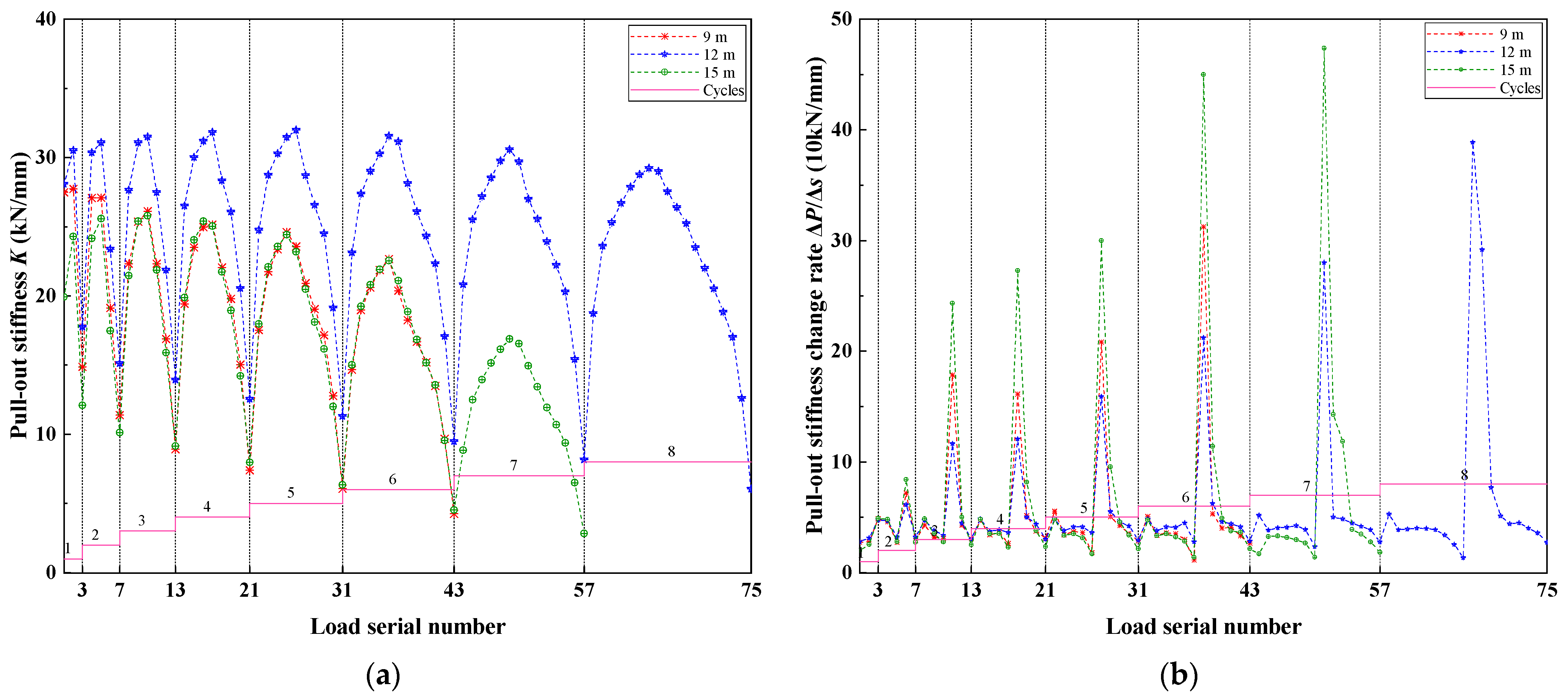
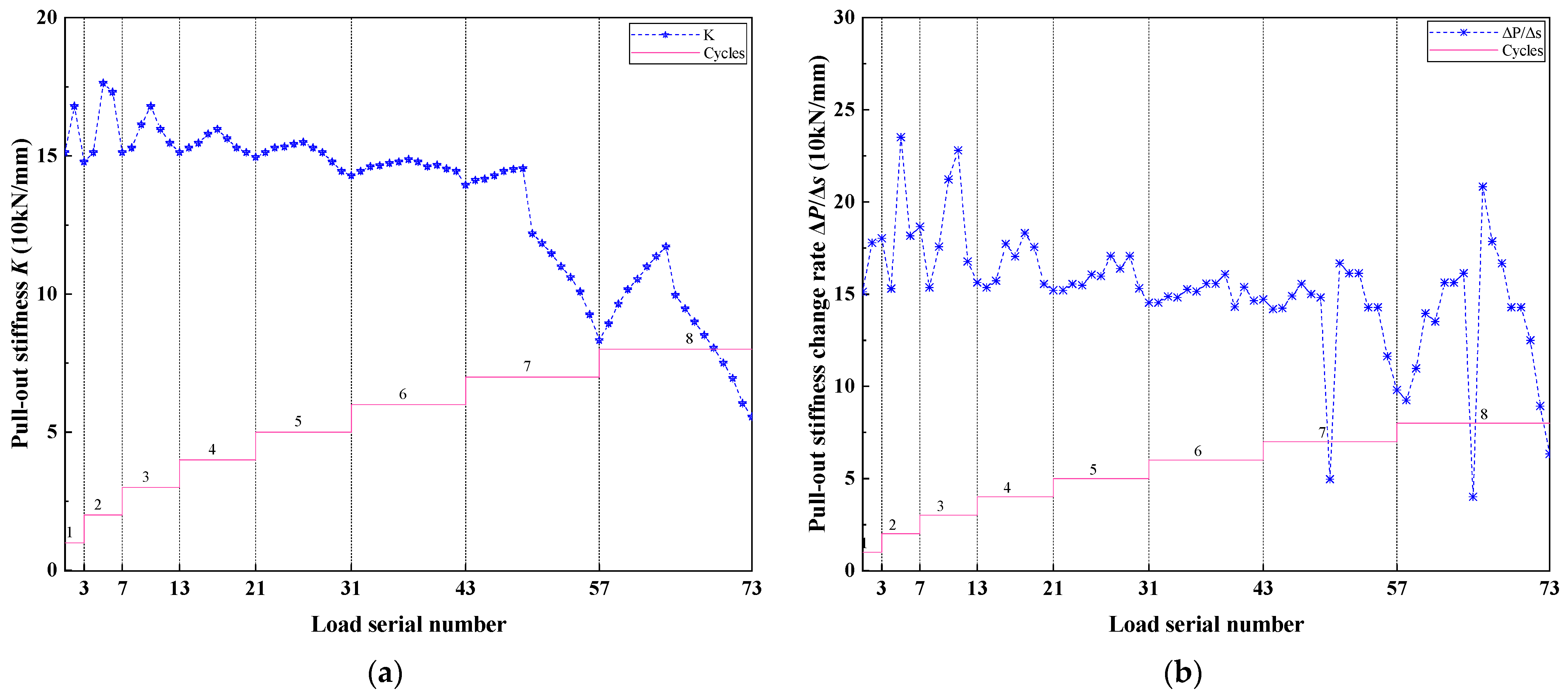
Figure 5 shows the variation law of pull-out stiffness K and its change rate ΔP/Δs with the test load and number of cycles during the test. It can be seen from Figure 5a that within each cycle of graded load, K gradually increased during loading and decreased during unloading, and under the same load, the value of K was smaller during unloading than loading. With an increase in the number of cycles, pull-out stiffness K under the same load basically shows a gradual decreasing trend as well. It can be seen from Figure 5b that in each cycle of graded load, during the loading process, the pull-out stiffness change rate ΔP/Δs first increased sharply, then decreased sharply, then gradually became stable, and finally decreased gradually. During the unloading process, ΔP/Δs increased sharply by several times, even more than 10 times, then rapidly decreased to about the average value, and finally decreased gradually. With an increase in the number of cycles, the multiple of ΔP/Δs during unloading also increased gradually, but the average value did not change much. It can be seen from Figure 5 that with the change of load and the increase in number of cycles, the pull-out stiffness of the bolt also changed regularly.

According to the parameters of this test, k_u = 198.5 MN was calculated. Referring to the assumption of Cai et al. [21], the influence radius of the bolt was taken as R = 35r_b, and the sidewall spring stiffness, calculated according to Equation (41), was k′_u = 25.8 MPa. The measured initial sidewall spring stiffnesses of the three bolts was 27.5, 28.1, and 19.9 MPa. Although these are all close to the results calculated by Equation (41), each bolt was different. If the same k′_u was used for simulation and analysis, the difference in pull-out stiffness among different bolts could not be seen. After analysis and calculation, the λ of the three bolts was between 0 and 0.4, so the working condition of λ ≈ 0 could be approximated for analysis.

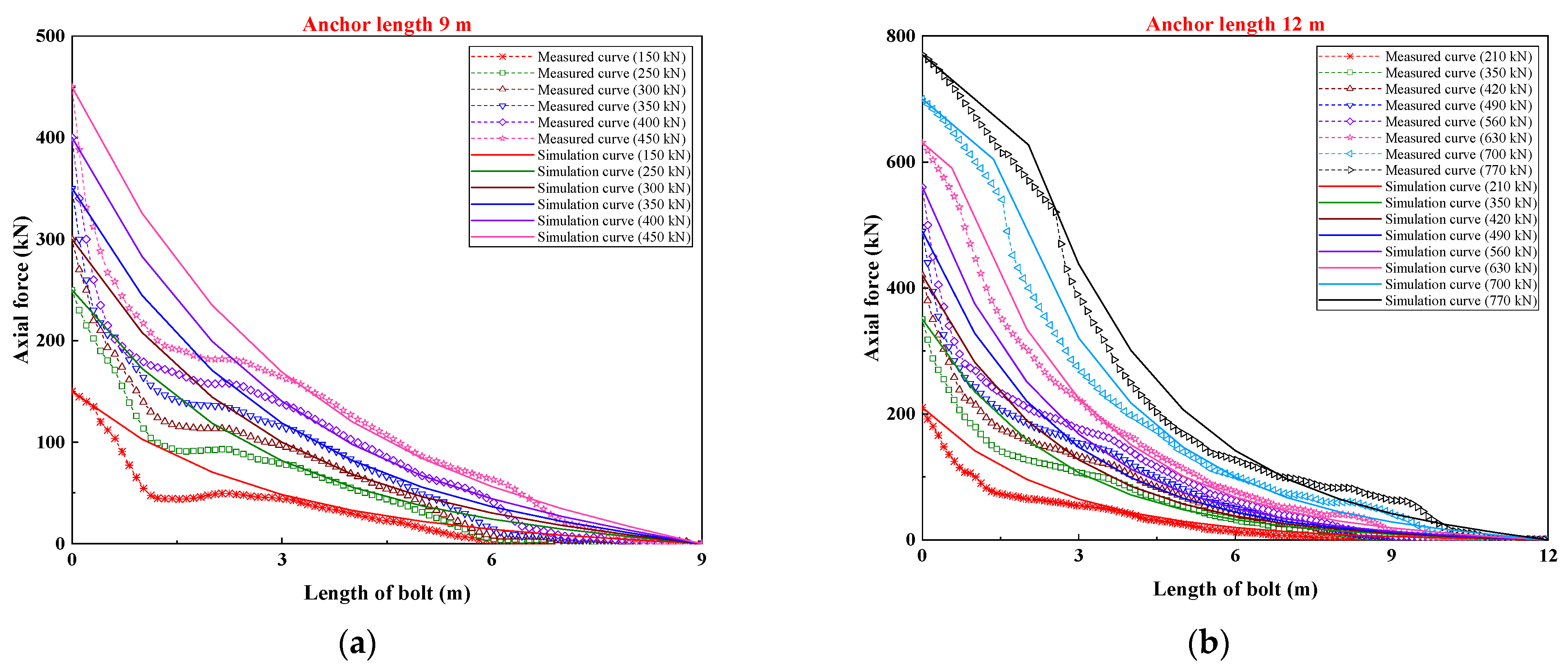
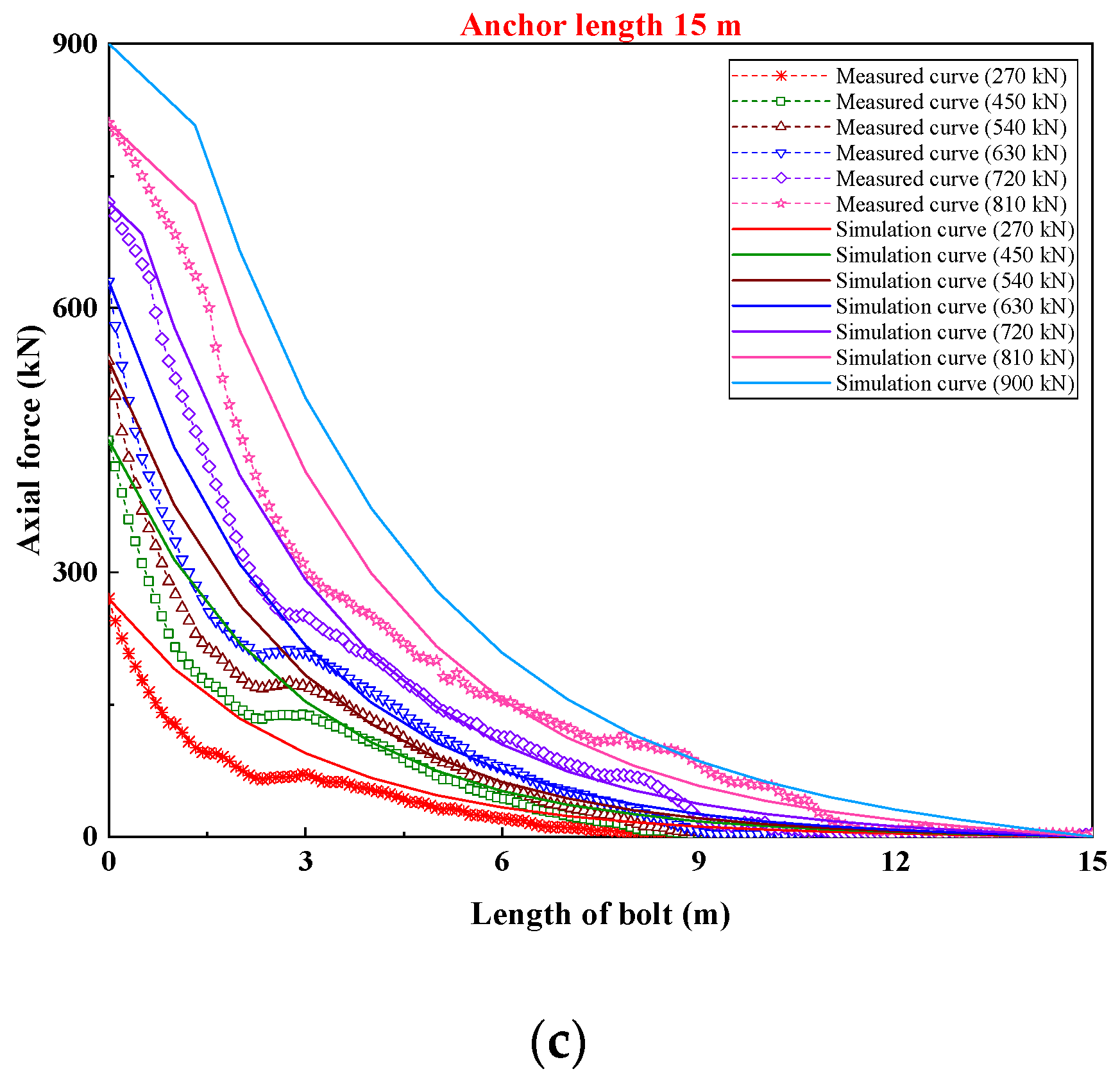
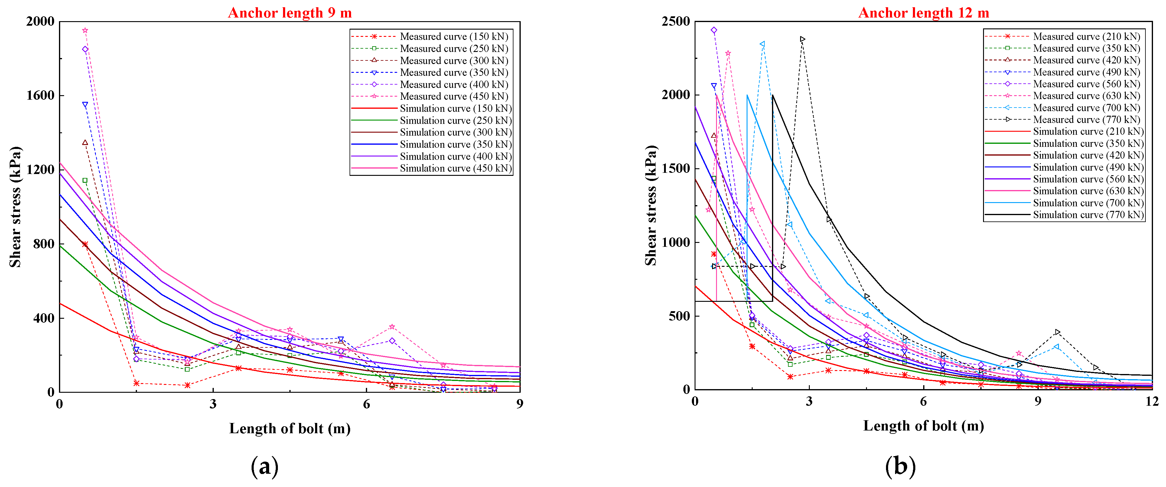
Figure 6 and Figure 7 show the comparison results of the measured axial force and shear-stress distribution curves of the three bolts and the simulated curves, respectively. According to the field test results, in the process of simulation analysis, the ultimate shear strength of the bonding interface between the bolt and the grout was taken as 2.0 MPa, and α was taken as 0.3. Then, the calculated ultimate friction resistance F_m and residual friction resistance F_r of the bolt bonding interface were 233.9 and 70.2 kN, respectively. The three bolts were analyzed and calculated using the model proposed in this paper, and the results are shown in

Table 1. Calculation results of the three bolts.

Bolt Length l (m)	Critical Failure Depth of Shear Plane xtj (m)	Ultimate Pull-Out Force P0max (kN)
9	5.6	940
12	8.8	1100
15	11.0	1300

.

It can be seen from Table 1 that the ultimate calculated values of pull-out force of these three bolts are all larger than the measured values, and there are large deviations. There are two main reasons for this problem. On the one hand, because the λ in this test is slightly larger, the working condition of λ ≈ 0 cannot be perfectly used for analysis. On the other hand, the ultimate measured pull-out force is determined according to the index of the creep rate not being more than 2.0 mm, and the value determined from this is much smaller than the calculated value. The pull-out performance of the bolt is mainly restricted by the two indexes of bearing capacity and deformation. When the deformation and creep rate of the bolt are large, it is obvious that more serious damage occurs. However, in fact, the bolt can still have a larger bearing capacity at this time. Therefore, in comparison, the ultimate pull-out force determined by the creep rate is safer and more reasonable, and the calculation and analysis results cannot be trusted blindly.

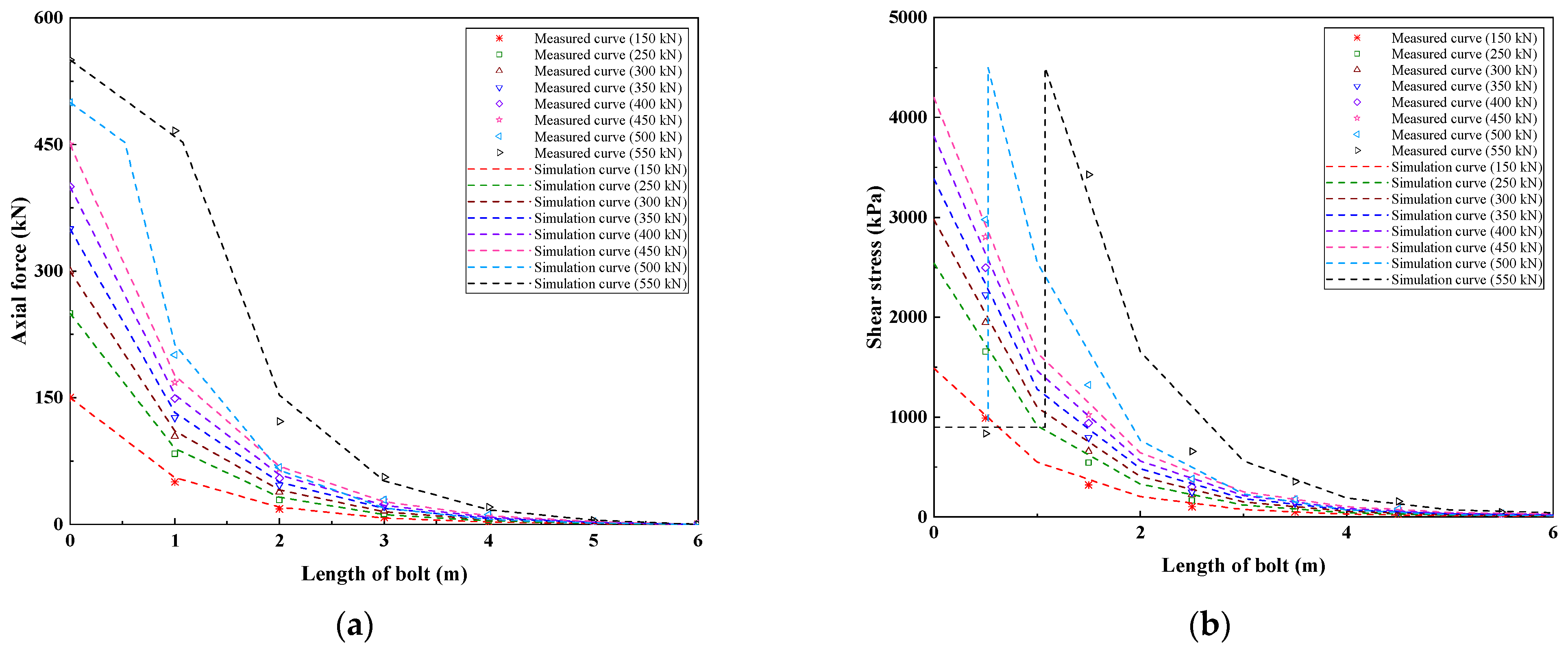
It can be seen from Figure 6 that the simulated axial force distribution curves of the three bolts are in good agreement with the measured curves. However, the measured values of the three bolts in the shallow part (about 0 to 3 m) are smaller than the simulated values, indicating that the three bolts are not uniformly stressed at this part, which may be related to the geological conditions of the site. It can be seen from Figure 6a that under a load of 450 kN, the simulation and measured results of the 9 m-long bolt show that the bolt has no obvious shear damage. It can be seen from Figure 6b that under loads of 630, 700, and 770 kN, the simulation and measured results of the 12 m-long bolt reflect that the bolt underwent obvious shear damage. The corresponding shear failure depth x_t of the simulated curves is 0.56, 1.36, and 2.04 m, respectively, while the corresponding x_t of the measured curves is 0.71, 1.53, and 2.55 m (slightly larger values). 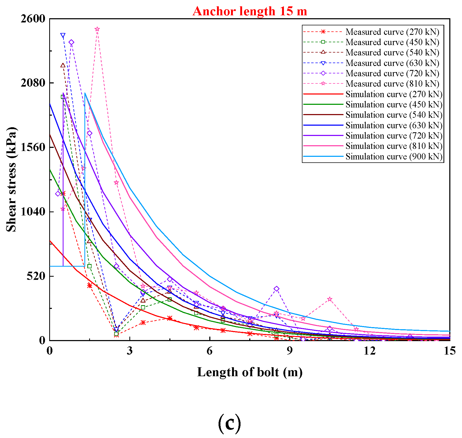It can be seen from Figure 6c that under loads of 720 and 810 kN, the simulated and measured results of the 15 m-long bolt reflect that the bolt underwent obvious shear damage. The corresponding x_t of the simulated curves is 0.51 and 1.32 m, while that of the measured curves is 0.61 and 1.53 m, respectively (the latter slightly larger than the former). Under a load of 900 kN, the simulated x_t is still 1.32 m, but stress–strain observation of the bolt was not carried out in the field test.

It can be seen from Figure 7 that when the bolts did not undergo shear failure, the measured shear stress of the three bolts was greater than the simulated value at about 0 to 1 m, and smaller than the simulated value at about 1 to 3 m. This shows that the shear stress of the three bolts attenuates too quickly in the range of 0 to 1 m, and the uneven stress on the bolts at this part is also observed. In other parts, the simulated shear stress distribution curves of the three bolts basically agree with the measured distribution curves. It can be seen from Figure 7b,c that the ultimate shear stress of the bonding interface is about 2.4 MPa and the residual shear stress is about 0.6 MPa, which are close to the values used in the simulation calculation.

In summary, although the model analysis results are slightly different from the measured results, the mechanical properties of fully grouted bolts under axial cyclic load in the working condition of λ ≈ 0 can still be well simulated.

5.2. Case 2 (Working Condition of λ ≈ 1)

For a certain fully grouted bolt, the following are known: bolt length l = 6 m; bolt radius r_b = 16 mm; elastic modulus of bolt E_b = 210 GPa; drilling radius r_g = 90 mm; mortar elastic modulus E_g = 20 GPa; mortar Poisson’s ratio μ_g = 0.25; shear modulus of rock soil around bolt G_r = 50 MPa. The test was loaded using a graded multi-cycle method, with a maximum test load of 550 kN, which was not loaded to the ultimate failure state. Strain gauges were installed at intervals of 1 m along the axial direction of the bolt to monitor axial strain.

Figure 8 shows the variation of K and ΔP/Δs with the test load and number of cycles during the test. It can be seen that under cyclic load, the variation rule of K in this case is the same as that in case 1, but the variation rule of ΔP/Δs is slightly different. This shows that under the two working conditions, the mechanical properties of the bolt under cyclic load are both similar and different. In the seventh and eighth cycles, K and ΔP/Δs both decreased sharply, indicating that shear failure occurred at the bond interface of the bolt at this time.

According to the parameters of this test, k_u = 168.9 MN and k′_u = 171.2 MPa were calculated, and the measured initial sidewall spring stiffness was 151.2 MPa. After analysis and calculation, the value of λ of the test bolt was between 0.8 and 1.2, so the working condition of λ ≈ 1 could be used for analysis. According to the field test results, in the process of simulation analysis, the ultimate shear strength of the bonding interface between the bolt and the grout was taken as 4.5 MPa, and α was taken as 0.2. Ultimate friction resistance F_m and residual friction resistance F_r of the bolt bonding interface calculated from this were 452.4 and 90.5 kN, respectively. The model in this paper was used to analyze and calculate the test bolt; the critical failure depth of shear plane x_tj and the ultimate pull-out force P_0max were about 4.7 m and 770 kN, respectively. In the field test, the bolt was not loaded to the ultimate failure state, so the actual ultimate pull-out force could not be obtained.

Figure 9 shows the comparison between the model analysis and field test results of the bolt. It can be seen from Figure 9b,c that the simulated axial force and shear stress distribution curves are in good agreement with the measured results. Under loads of 500 and 550 kN, the simulation and actual measurement results show that obvious shear failure occurred in the shallow part of the bolt, and the corresponding shear-failure depth x_t was 0.53 and 1.08 m, respectively. Due to the sparseness of bolt-stress-monitoring points, the measured results cannot reflect the shear-failure depth and ultimate shear-stress of the bond interface. In summary, the analytical model in this paper is more suitable for simulating the mechanical behavior of fully grouted bolts under axial cyclic load in the working condition of λ ≈ 1.

6. Conclusions

Based on the idea of discretization, force analysis of bolts was carried out, and the spring element method for bolt analysis is put forward. In addition, the relationship between the displacement, axial force, and side resistance distribution functions of the bonding interface is established.

Assuming that the bolt and the rock soil mass are connected by tangential linear springs, the load-transfer model of the fully grouted bolt is established by using the spring element method. Considering the two situations before and after the damage of the sidewall spring, the displacement, axial force, and shear-stress distribution functions of the bolt are derived. Through further analysis, it is found that the model in this paper is more suitable for simulation analysis in the two working conditions of λ ≈ 0 and λ ≈ 1. Furthermore, the relationship between the sidewall spring stiffness and the pull-out stiffness of the bolt was established under these two working conditions, and the variation characteristics of the sidewall spring stiffness under cyclic load were analyzed.

Using two test cases under the two working conditions of λ ≈ 0 and λ ≈ 1, the variation law of pull-out stiffness and its change rate with the test load and number of cycles was analyzed, and the analytical model proposed in this study was discussed and verified. It was verified by tests that the analytical model in this paper is more suitable for simulating the mechanical behavior characteristics of fully grouted bolts under axial cyclic load in working conditions of λ ≈ 0 and λ ≈ 1, and comparing the two, the model is more applicable to λ ≈ 1.

This study contributes to a comprehensive understanding of the mechanical behavior of fully grouted bolts under axial cyclic load.

References

1. Ren, F.F.; Yang, Z.J.; Chen, J.F.; Chen, W.W. An analytical analysis of the full-range behaviour of grouted rock bolts based on a tri-linear bond-slip mode1. Constr. Build. Mater. 2010, 24, 361–370. [Google Scholar] [CrossRef]
2. Zou, J.F.; Zhang, P.H. Analytical model of fully grouted bolts in pull-out tests and in situ rock masses. Int. J. Rock Mech. Min. Sci. 2019, 113, 278–294. [Google Scholar] [CrossRef]
3. Ma, S.; Nemcik, J.; Aziz, N. An analytical model of fully grouted rock bolts subjected to tensile load. Constr. Build. Mater. 2013, 49, 519–526. [Google Scholar] [CrossRef]
4. Fujita, K. A method to predict the load-displacement relationship of ground anchors. In Proceedings of the 9th International Conference on Soil Mechanics and Foundation Engineering, Tokyo, Japan, 10–15 July 1977. [Google Scholar]
5. Stillborg, B. Experimental Investigation of Steel Cables for Rock Reinforcement in Hard Rock. Ph.D. Dissertation, Lulea University of Technology, Lulea, Sweden, 1984. [Google Scholar]
6. Su, W.; Fragaszy, R.J. Uplift testing of model anchors. J. Geotech. Eng. Div. 1988, 114, 961–983. [Google Scholar] [CrossRef]
7. Hyett, A.J.; Bawden, W.F.; Relchert, R.D. The effect of rock mass confinement on the bond strength of fully grouted cable bolts. Int. J. Rock Mech. Min. Sci. Geomech. Abstr. 1992, 29, 503–524. [Google Scholar] [CrossRef]
8. Kilic, A.; Yasar, E.; Celik, A.G. Effect of grout properties on the pull-out load capacity of fully grouted rock bolt. Tunn. Undergr. Sp. Tech. 2002, 17, 355–362. [Google Scholar] [CrossRef]
9. Kim, N.K. Performance of tension and compression anchors in weathered soil. J. Geotech. Geoenviron. Eng. 2003, 129, 1138–1150. [Google Scholar] [CrossRef]
10. Huang, M.H.; Zhou, Z.; Huang, Y.; Ou, J.P. A distributed self-sensing FRP anchor with built-in optical fiber sensor. Measurement 2013, 46, 1363–1370. [Google Scholar] [CrossRef]
11. Phillips, S.H.E. Factors Affecting the Design of Anchorages in Rock; Cementation Research Ltd.: London, UK, 1970. [Google Scholar]
12. Farmer, I.W. Stress distribution along a resin grouted rock anchor. Int. J. Rock Mech. Min. Sci. Geomech. Abstr. 1975, 12, 347–351. [Google Scholar] [CrossRef]
13. Wijk, G. A theoretical remark on the stress field around prestressed rock bolts. Int. J. Rock Mech. Min. Sci. Geomech. Abstr. 1978, 15, 289–294. [Google Scholar] [CrossRef]
14. Aydan, O.; Ichikawa, Y.; Kawamoto, T. Load bearing capacity and stress distributions in along rock bolts with inelastic behaviour of interfaces. In Proceeding of the 5th International Conference on Numerical Methods in Geomechanics, Nagoya, Japan, 1–5 April 1985. [Google Scholar]
15. Li, C.; Stillborg, B. Analytical models for rock bolts. Int. J. Rock Mech. Min. Sci. 1999, 36, 1013–1029. [Google Scholar] [CrossRef]
16. Chen, J.; Saydam, S.; Hagan, P. An analytical model of the load transfer behavior of fully grouted cable bolts. Constr. Build. Mater. 2015, 101, 1006–1015. [Google Scholar] [CrossRef]
17. Li, D.; Cai, M.; Masoumi, H. A constitutive model for modified cable bolts exhibiting cone shaped failure mode. Int. J. Rock Mech. Min. Sci. 2021, 145, 104855. [Google Scholar] [CrossRef]
18. Jahangir, E.; Blanco-Martín, L.; Hadj-Hassen, F.; Tijani, M. Development and application of an interface constitutive model for fully grouted rock-bolts and cable-bolts. J. Rock Mech. Geotech. Eng. 2021, 13, 811–819. [Google Scholar] [CrossRef]
19. Malvar, L.J. Bond reinforcement under controlled confinement. ACI Mater. J. 1992, 89, 593–601. [Google Scholar]
20. Moosavi, M.; Khosravi, A.; Jafari, A. A laboratory study of bond failure mechanism in deformed rock bolts using a modified Hoek cell. In Proceedings of the 2001 ISRM International Symposium-Second Asian Rock Mechanics Symposium (ISRM 2001-2nd ARMS), Beijing, China, 11–14 September 2001. [Google Scholar]
21. Cai, Y.; Esakia, T.; Jiang, Y.J. A rock bolt and rock mass interaction model. Int. J. Rock Mech. Min. Sci. Geomech. Abstr. 2004, 41, 1055–1067. [Google Scholar] [CrossRef]
Figure 1. Schematic diagram of discretization of free rod.
Minerals 12 01566 g001
Figure 2. Schematic diagram of discretization of bolt.
Minerals 12 01566 g002
Figure 3. Force analysis diagram of the ith spring element.
Minerals 12 01566 g003
Figure 4. Load-transfer model.
Minerals 12 01566 g004
Figure 5. Variation of K and ΔPs with test load and number of cycles during the test (working condition of λ ≈ 0). (a) Variation of pull-out stiffness K; (b) variation of pull-out stiffness change rate ΔPs.
Minerals 12 01566 g005
Figure 6. Comparison of measured axial force distribution curve and simulated curve: (a) 9 m-long bolt; (b) 12 m-long bolt; (c) 15 m-long bolt.
Minerals 12 01566 g006aMinerals 12 01566 g006b
Figure 7. Comparison of measured shear stress distribution curve and simulated curve: (a) 9 m-long bolt; (b) 12 m-long bolt; (c) 15 m-long bolt.
Minerals 12 01566 g007aMinerals 12 01566 g007b
Figure 8. Variation of K and ΔPs with test load and number of cycles during the test (working condition of λ ≈ 1): (a) pull-out stiffness K; (b) pull-out stiffness change rate ΔPs.
Minerals 12 01566 g008
Figure 9. Comparison of model analysis and test results: (a) axial force distribution; (b) shear stress distribution.
Minerals 12 01566 g009