Author Contributions
Methodology, data creation, investigation, writing-original draft, Z.C.; methodology, supervision, writing-review and editing, J.Z.; investigation, formal analysis, writing-review and editing, K.L.; formal analysis, investigation, M.L. All authors have read and agreed to the published version of the manuscript.
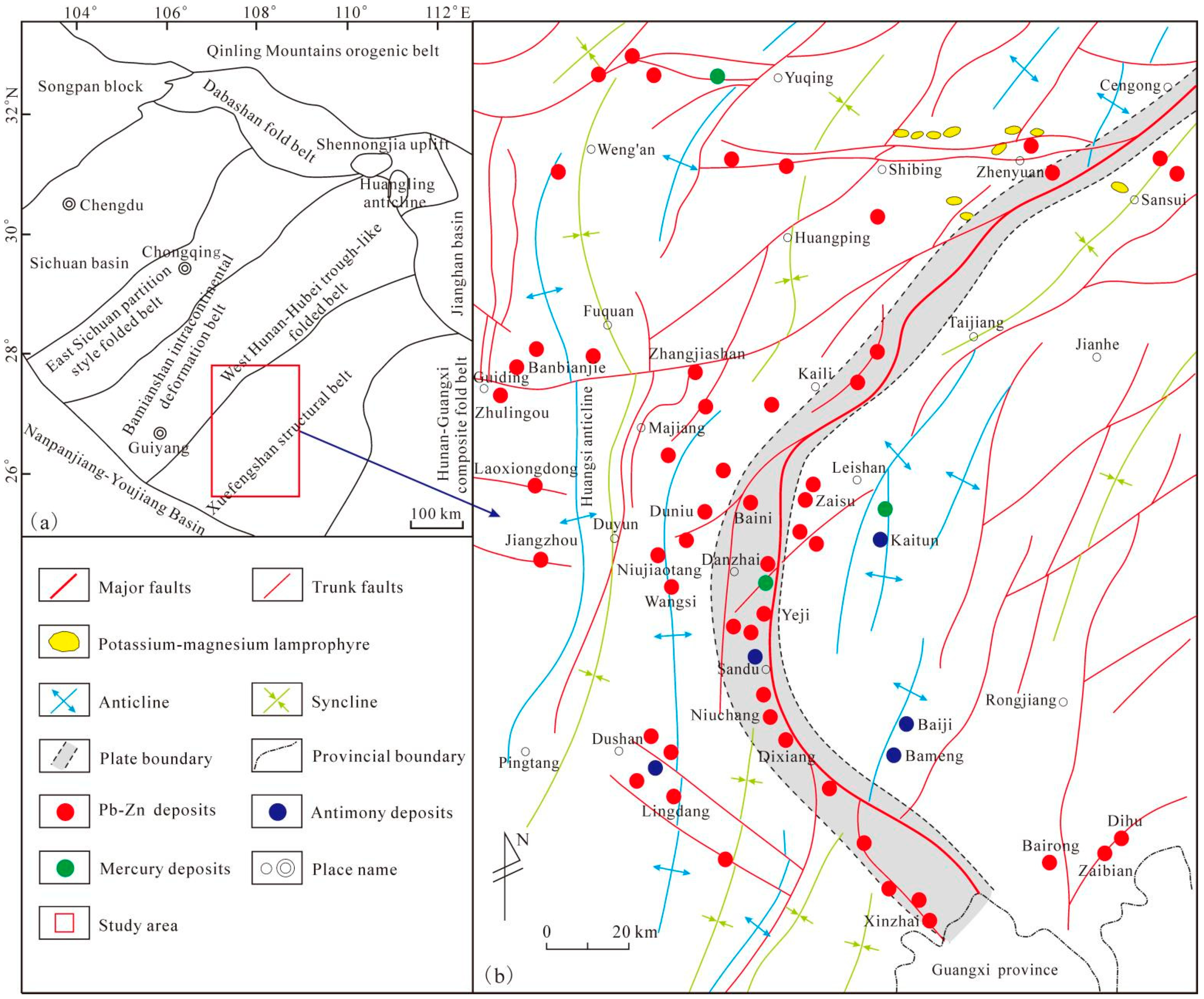
Figure 1.
Geotectonic position of the study area: (
a) according to Ref. [
3] and fault structures, deposits distribution map (
b): according to Ref. [
26].
Figure 1.
Geotectonic position of the study area: (
a) according to Ref. [
3] and fault structures, deposits distribution map (
b): according to Ref. [
26].
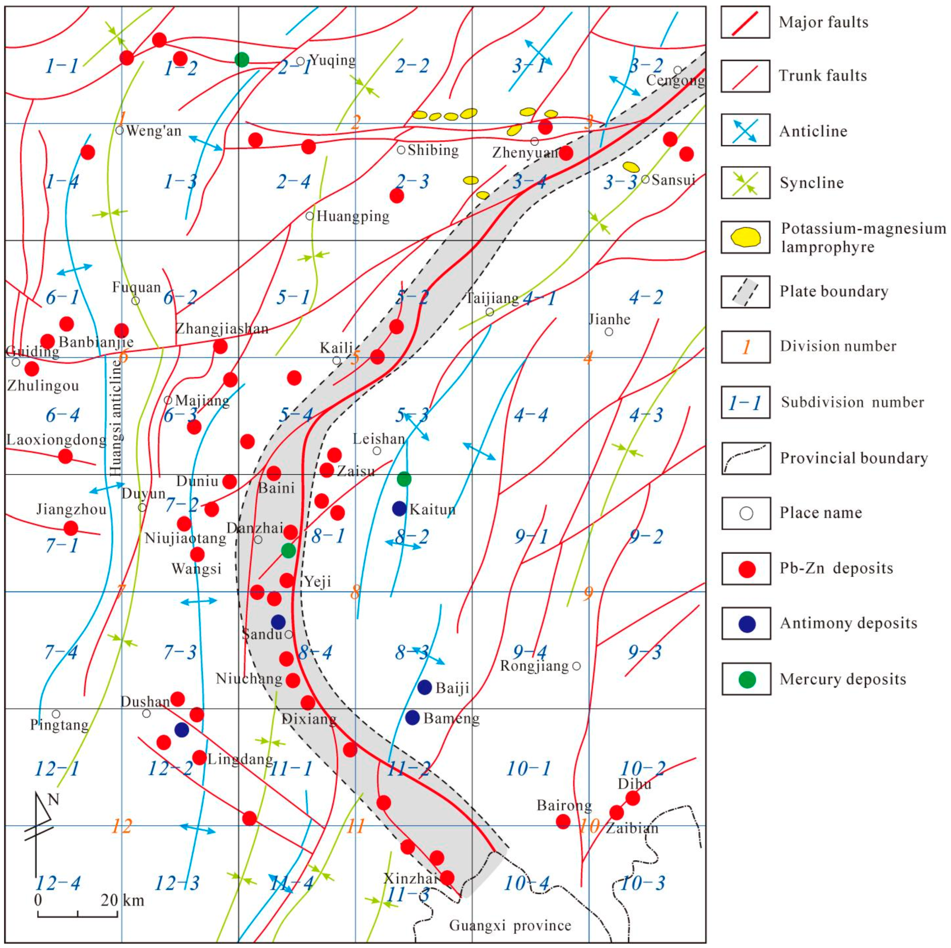
Figure 2.
Computation partition map of fractal dimension (modified from Ref. [
26]).
Figure 2.
Computation partition map of fractal dimension (modified from Ref. [
26]).
Figure 3.
Linear fitting diagrams of the capacity dimension (CPD) calculation for faults in the eastern Guizhou Pb–Zn metallogenic belt (EGMB). The lnr versus lnN(r) plots of CPD data for (a) Integrated faults; (b) NE-trending faults; (c) NW-trending faults; (d) Near-SN-trending faults; (e) Near-EW-trending faults; (f) Major faults; and (g) Plate contact transition zone, showing their linear regression parameters.
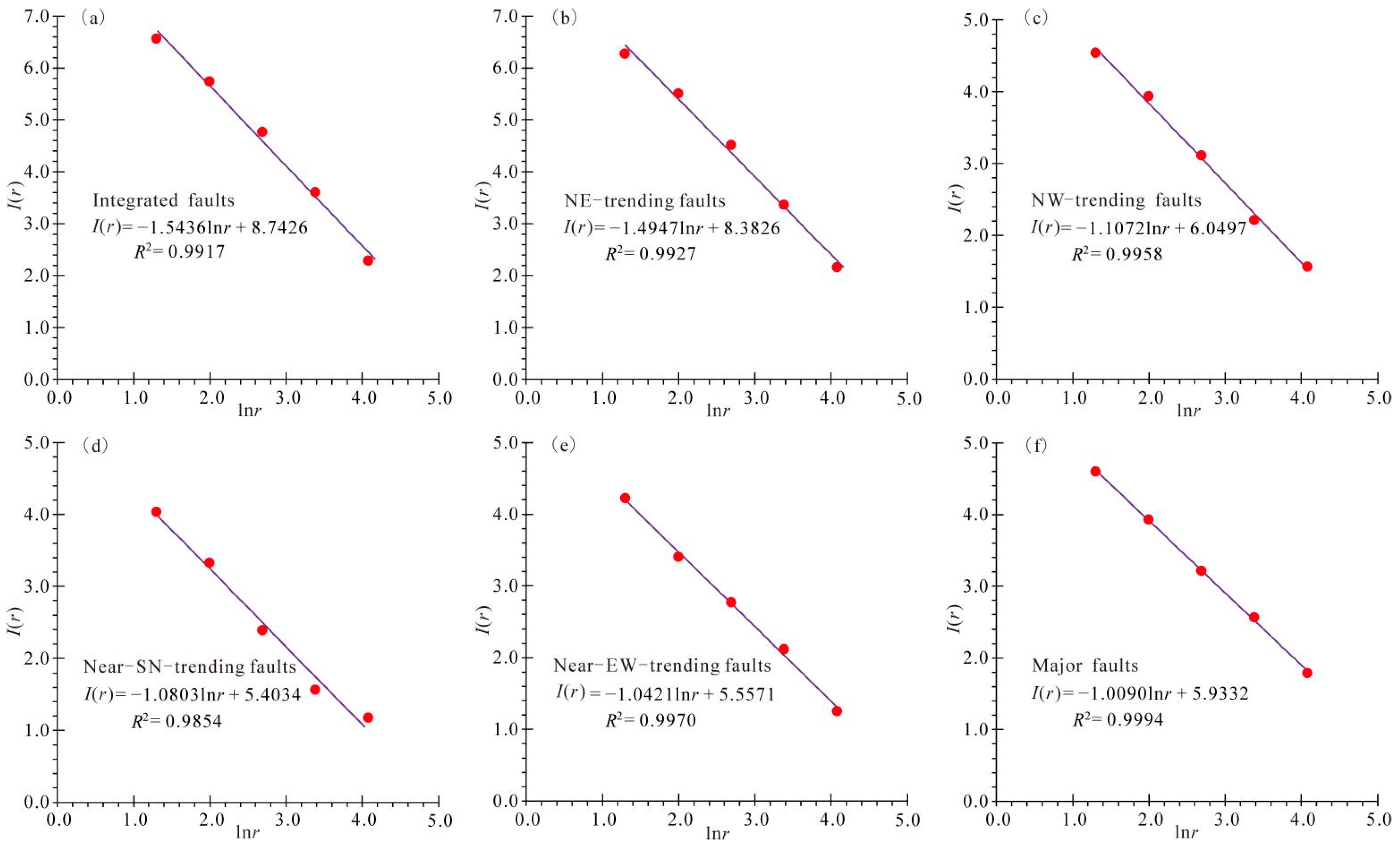
Figure 4.
Linear fitting diagrams of the information dimension (IND) calculation for faults in the eastern Guizhou Pb–Zn metallogenic belt (EGMB). The lnr versus I(r) plots of IND data for (a) Integrated faults; (b) NE-trending faults; (c) NW-trending faults; (d) Near-SN-trending faults; (e) Near-EW-trending faults; and (f) Major faults, showing their linear regression parameters.
Figure 5.
Linear fitting diagrams for the correlation dimension (CRD) calculation of faults in the eastern Guizhou Pb–Zn metallogenic belt (EGMB). The lnr versus I(r) plots of CRD data for (a) Integrated faults; (b) NE-trending faults; (c) NW-trending faults; (d) Near-SN-trending faults; (e) Near-EW-trending faults; and (f) Major faults, showing their linear regression parameters.
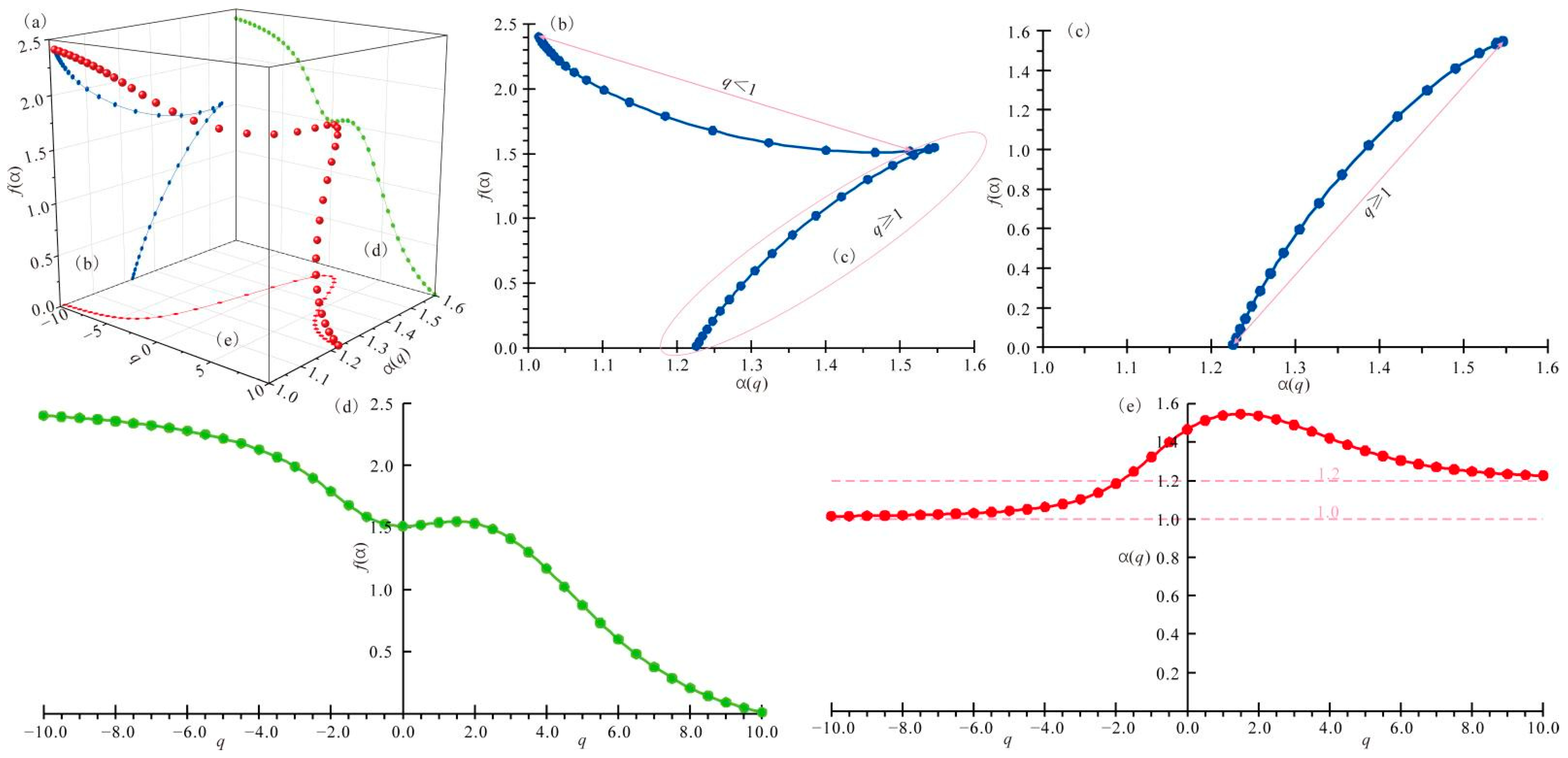
Figure 6.
Multi-fractal spectrum of faults in the study area. (a) 3-D plot of q, α(q), f(α), showing points (q, α(q), f(α)) in the three-dimensional coordinate system is a spiral; (b) 2-D plot of α(q), f(α), showing the curve connected by points (α(q), f(α)) is not a common parabolic (or hook) shape with downward opening, but a combination of two semi-parabolic shapes with opposite opening directions; (c) When the q-order moment ranges from 1 to 10, the curve connecting the points (α(q), f(α)) is a typical semi-parabolic shape; (d) f(α) ranges from 0.0120 to 2.4020, and decreases as a whole and increases locally with the increase of the order moment q; and (e) the singularity index α(q) first increases and then decreases with the increase of the order moment q.
Figure 7.
Linear fitting graph for spatial distribution fractal dimensions (SDD) calculation of ore deposits.
Figure 7.
Linear fitting graph for spatial distribution fractal dimensions (SDD) calculation of ore deposits.
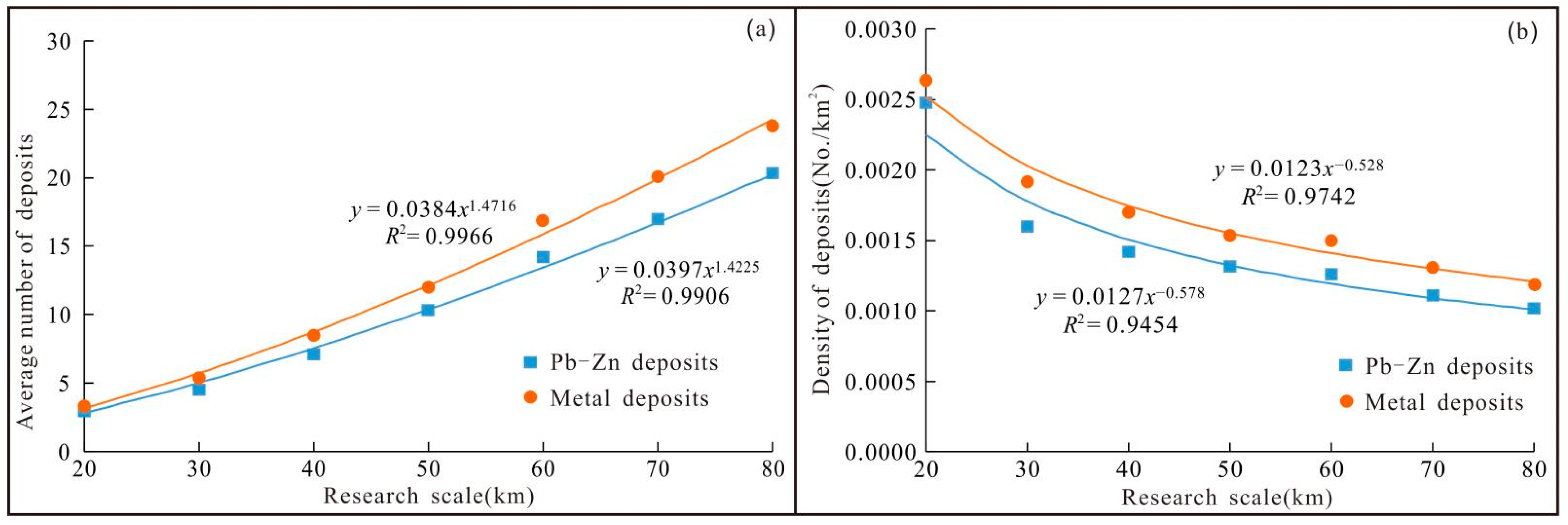
Figure 8.
Fitting diagram of fractal distribution for deposit number (a) and density (b).
Figure 8.
Fitting diagram of fractal distribution for deposit number (a) and density (b).
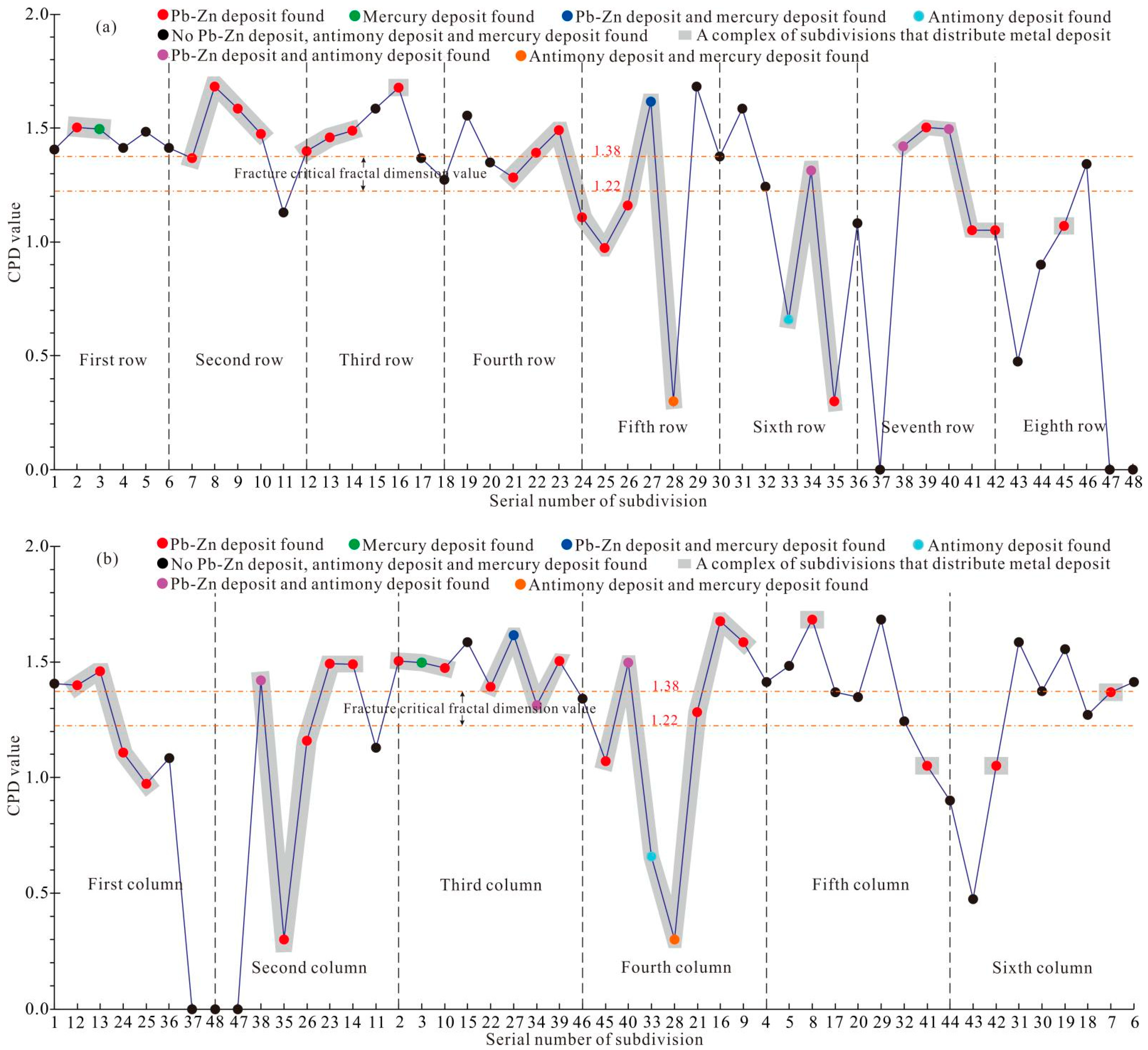
Figure 9.
Vertical and horizontal wave graphs of fractal dimensions. (a) Horizontal wave graphs of fractal dimensions; and (b) Vertical wave graphs of fractal dimensions.
Figure 9.
Vertical and horizontal wave graphs of fractal dimensions. (a) Horizontal wave graphs of fractal dimensions; and (b) Vertical wave graphs of fractal dimensions.
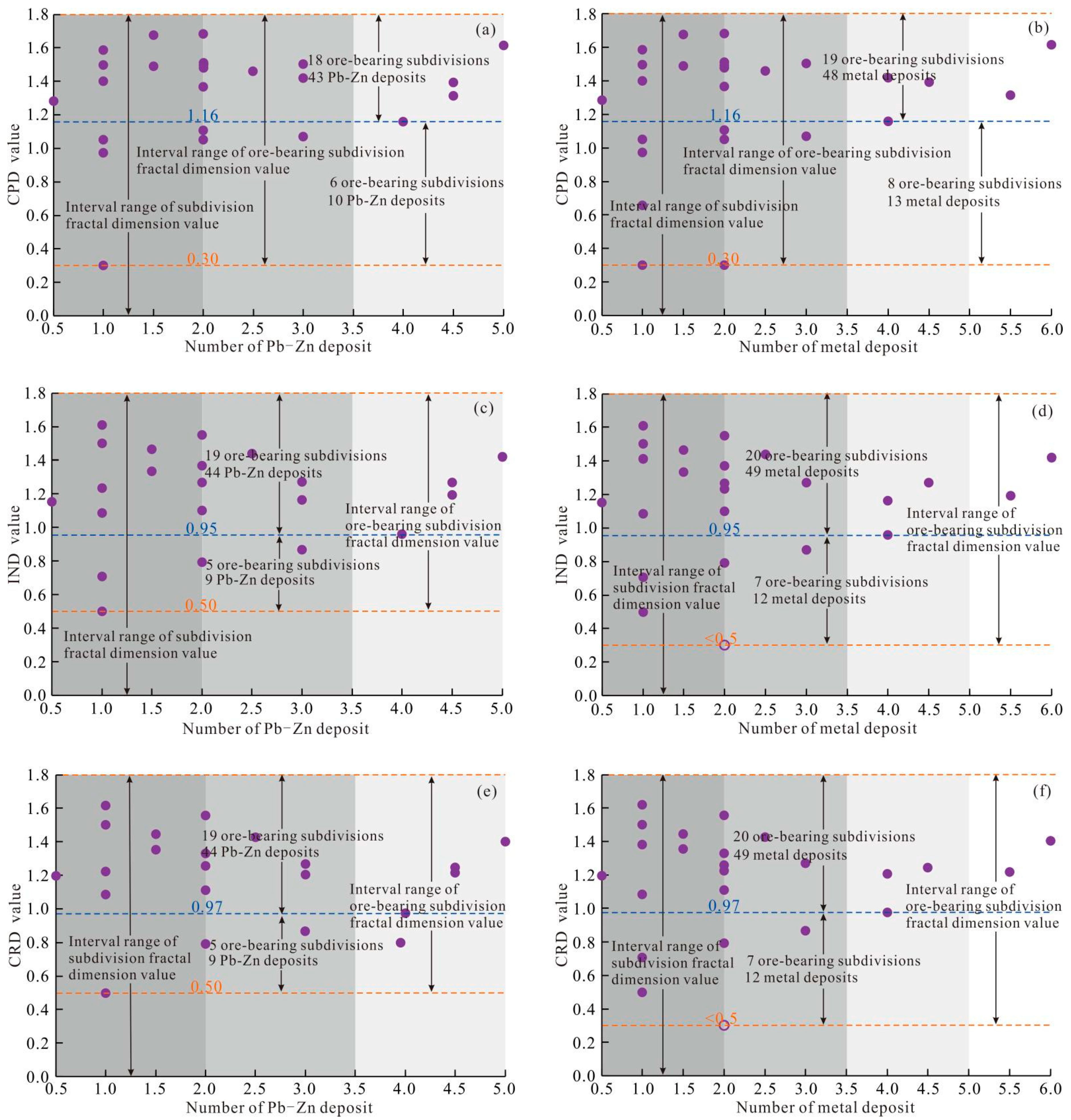
Figure 10.
Subdivision projection maps of deposit quantity versus fractal dimension. (a) Subdivision projection maps of Pb–Zn deposit quantity versus CPD; (b) Subdivision projection maps of all metals deposits quantity versus CPD; (c) Subdivision projection maps of Pb–Zn deposit quantity versus IND; (d) Subdivision projection maps of all metals deposits quantity versus IND; (e) Subdivision projection maps of Pb–Zn deposit quantity versus CRD; and (f) Subdivision projection maps of all metals deposits quantity versus CRD.
Figure 11.
Different types of fractal dimension projection maps of subdivisions. (a) 3-D plot of CPD, IND, CRD of ore-bearing subdivision; (b) CPD versus IND plot of ore-bearing subdivision; (c) CPD versus CRD plot of ore-bearing subdivision; and (d) IND versus CRD plot of ore-bearing subdivision.
Figure 11.
Different types of fractal dimension projection maps of subdivisions. (a) 3-D plot of CPD, IND, CRD of ore-bearing subdivision; (b) CPD versus IND plot of ore-bearing subdivision; (c) CPD versus CRD plot of ore-bearing subdivision; and (d) IND versus CRD plot of ore-bearing subdivision.
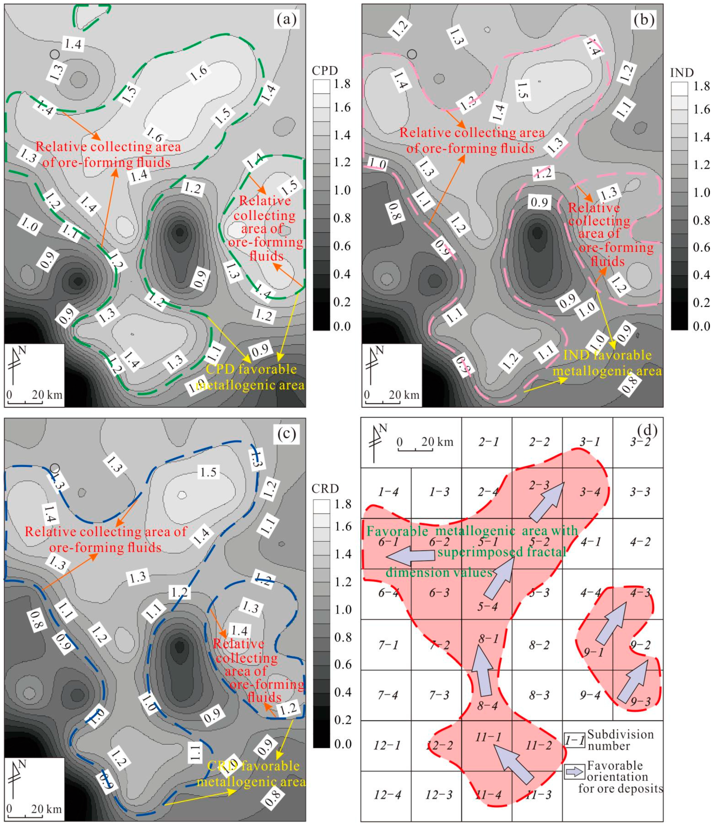
Figure 12.
Fractal dimension favorable mining area. (a) CPD of fault favorable mining area; (b) IND of fault favorable mining area; (c) CRD of fault favorable mining area; and (d) Comprehensive consideration of fault fractal dimension value for favorable metallogenic area.
Figure 12.
Fractal dimension favorable mining area. (a) CPD of fault favorable mining area; (b) IND of fault favorable mining area; (c) CRD of fault favorable mining area; and (d) Comprehensive consideration of fault fractal dimension value for favorable metallogenic area.
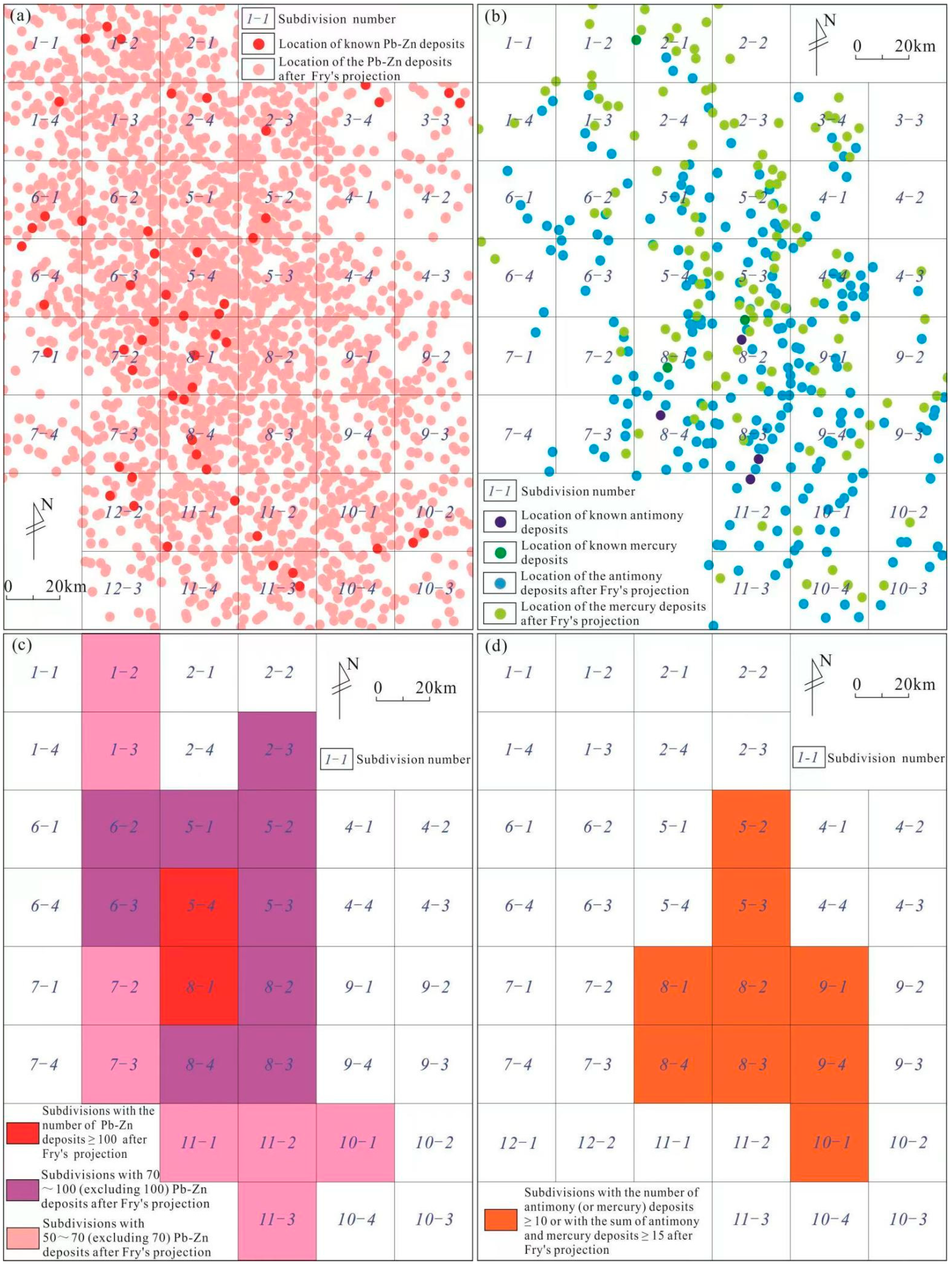
Figure 13.
Fry analysis map of the deposit. (a) Fry analysis diagram of Pb–Zn deposits; (b) Fry analysis diagram of Sb–Hg deposits; (c) Fry point distribution map of Pb–Zn deposits; and (d) Fry point distribution map of Sb–Hg deposits.
Figure 13.
Fry analysis map of the deposit. (a) Fry analysis diagram of Pb–Zn deposits; (b) Fry analysis diagram of Sb–Hg deposits; (c) Fry point distribution map of Pb–Zn deposits; and (d) Fry point distribution map of Sb–Hg deposits.
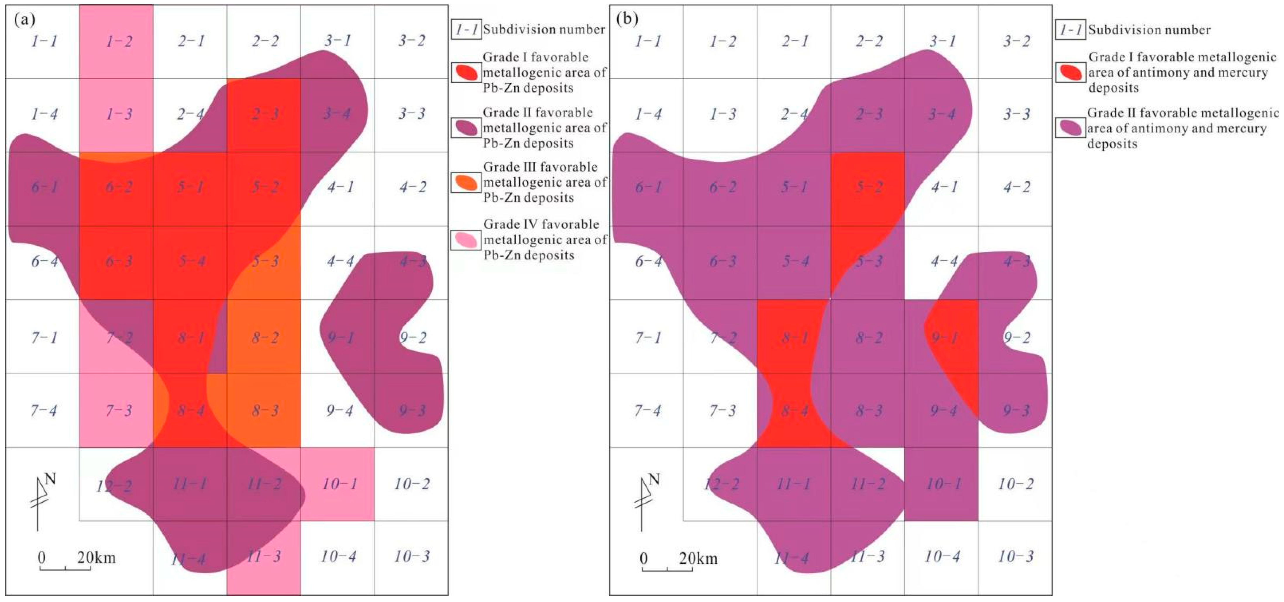
Figure 14.
Distribution map of comprehensive favorable metallogenic areas. (a) Distribution map of Pb–Zn deposits comprehensive favorable metallogenic areas and (b) Distribution map of Sb–Hg deposits comprehensive favorable metallogenic areas.
Figure 14.
Distribution map of comprehensive favorable metallogenic areas. (a) Distribution map of Pb–Zn deposits comprehensive favorable metallogenic areas and (b) Distribution map of Sb–Hg deposits comprehensive favorable metallogenic areas.
Table 1.
Statistical table of calculation parameters of fractal dimensions for fault structures in the eastern Guizhou Pb–Zn metallogenic belt (EGMB).
Table 1.
Statistical table of calculation parameters of fractal dimensions for fault structures in the eastern Guizhou Pb–Zn metallogenic belt (EGMB).
| Category | CPD, D0 | IND, D1 | CRD, D2 |
|---|
| r (km) | N(r) | lnr | lnN(r) | r (km) | lnr | I(r) | r (km) | lnr | I(r) |
|---|
| Integrated faults | 58.716 | 12 | 4.073 | 2.485 | 58.716 | 4.073 | 2.366 | 58.716 | 4.073 | 2.291 |
| 29.358 | 45 | 3.380 | 3.807 | 29.358 | 3.380 | 3.692 | 29.358 | 3.380 | 3.606 |
| 14.679 | 146 | 2.686 | 4.984 | 14.679 | 2.686 | 4.874 | 14.679 | 2.686 | 4.767 |
| 7.340 | 368 | 1.993 | 5.908 | 7.340 | 1.993 | 5.836 | 7.340 | 1.993 | 5.743 |
| 3.670 | 785 | 1.300 | 6.666 | 3.670 | 1.300 | 6.628 | 3.670 | 1.300 | 6.572 |
| NE-trending faults | 58.716 | 11 | 4.073 | 2.398 | 58.716 | 4.073 | 2.257 | 58.716 | 4.073 | 2.165 |
| 29.358 | 37 | 3.380 | 3.611 | 29.358 | 3.380 | 3.475 | 29.358 | 3.380 | 3.369 |
| 14.679 | 114 | 2.686 | 4.736 | 14.679 | 2.686 | 4.628 | 14.679 | 2.686 | 4.518 |
| 7.340 | 281 | 1.993 | 5.638 | 7.340 | 1.993 | 5.582 | 7.340 | 1.993 | 5.509 |
| 3.670 | 570 | 1.300 | 6.346 | 3.670 | 1.300 | 6.316 | 3.670 | 1.300 | 6.275 |
| NW-trending faults | 58.716 | 6 | 4.073 | 1.792 | 58.716 | 4.073 | 1.676 | 58.716 | 4.073 | 1.569 |
| 29.358 | 11 | 3.380 | 2.398 | 29.358 | 3.380 | 2.307 | 29.358 | 3.380 | 2.213 |
| 14.679 | 25 | 2.686 | 3.219 | 14.679 | 2.686 | 3.170 | 14.679 | 2.686 | 3.114 |
| 7.340 | 53 | 1.993 | 3.970 | 7.340 | 1.993 | 3.957 | 7.340 | 1.993 | 3.937 |
| 3.670 | 95 | 1.300 | 4.554 | 3.670 | 1.300 | 4.550 | 3.670 | 1.300 | 4.544 |
| Near-SN-trending faults | 58.716 | 4 | 4.073 | 1.386 | 58.716 | 4.073 | 1.273 | 58.716 | 4.073 | 1.176 |
| 29.358 | 6 | 3.380 | 1.792 | 29.358 | 3.380 | 1.676 | 29.358 | 3.380 | 1.569 |
| 14.679 | 13 | 2.686 | 2.565 | 14.679 | 2.686 | 2.479 | 14.679 | 2.686 | 2.392 |
| 7.340 | 30 | 1.993 | 3.401 | 7.340 | 1.993 | 3.370 | 7.340 | 1.993 | 3.329 |
| 3.670 | 64 | 1.300 | 4.159 | 3.670 | 1.300 | 4.122 | 3.670 | 1.300 | 4.040 |
| Near-EW-trending faults | 58.716 | 4 | 4.073 | 1.386 | 58.716 | 4.073 | 1.311 | 58.716 | 4.073 | 1.259 |
| 29.358 | 10 | 3.380 | 2.303 | 29.358 | 3.380 | 2.211 | 29.358 | 3.380 | 2.120 |
| 14.679 | 18 | 2.686 | 2.890 | 14.679 | 2.686 | 2.834 | 14.679 | 2.686 | 2.774 |
| 7.340 | 34 | 1.993 | 3.526 | 7.340 | 1.993 | 3.469 | 7.340 | 1.993 | 3.409 |
| 3.670 | 71 | 1.300 | 4.263 | 3.670 | 1.300 | 4.248 | 3.670 | 1.300 | 4.226 |
| Major faults | 58.716 | 6 | 4.073 | 1.792 | 58.716 | 4.073 | 1.792 | 58.716 | 4.073 | 1.792 |
| 29.358 | 13 | 3.380 | 2.565 | 29.358 | 3.380 | 2.565 | 29.358 | 3.380 | 2.565 |
| 14.679 | 25 | 2.686 | 3.219 | 14.679 | 2.686 | 3.219 | 14.679 | 2.686 | 3.219 |
| 7.340 | 51 | 1.993 | 3.932 | 7.340 | 1.993 | 3.932 | 7.340 | 1.993 | 3.932 |
| 3.670 | 100 | 1.300 | 4.605 | 3.670 | 1.300 | 4.605 | 3.670 | 1.300 | 4.605 |
| Plate contact transition zone | 58.716 | 8 | 4.073 | 2.079 | - |
| 29.358 | 17 | 3.380 | 2.833 |
| 14.679 | 43 | 2.686 | 3.761 |
| 7.340 | 112 | 1.993 | 4.718 |
| 3.670 | 328 | 1.300 | 5.793 |
Table 2.
Statistical table of fractal dimension for fault structures in some areas of China.
Table 2.
Statistical table of fractal dimension for fault structures in some areas of China.
| Region | Scale Interval
(km) | CPD, D0 | IND, D1 | CRD, D2 | Reference |
|---|
| Activity Area of Continent in China (Diwa Area) | 8–256 | 1.236–1.624 | - | - | [49] |
| Stable Area of Continent in China (platform area) | 8–256 | 0.827–1.074 | - | - |
| Yungui Activity Area | 8–256 | 1.332 | - | - |
| China Continent | 8–256 | 1.493 | - | - |
| Shell Binding Site | 8–256 | >1.5 | - | - |
| Sichuan-Yunnan-Guizhou Pb–Zn Metallogenic Province | 9.336–149.373 | 1.5395 | - | - | [54] |
| Zhaxikang Ore Concentration Area | 0.073–4.7 | 1.249 | - | - | [75] |
| Gudui–Longzi Region, Tibet | 1.875–30 | 1.678 | - | - | [78] |
| Tongling Ore Concentration Area | 0.1–3 | 1.29 | - | - | [52] |
| Jiaojia District, Jiaodong | 0.50–16.00 | 1.3507 | - | - | [79] |
| Sanshandao-Cangshang Gold Mine Field in Jiaojia District | 0.25–4.00 | 1.0103 | - | - |
| Jiaojia Gold Mine Field in Jiaojia District | 0.25–4.00 | 1.3198 | - | - |
| Canzhuang-Lingshangou Gold Mine Field in Jiaojia District | 0.25–4.00 | 1.3656 | - | - |
| Xiyou–Zhuqiao Area in Jiaojia District (Mineral-free Area) | 0.25–4.00 | 1.1315 | - | - |
| Kangguertage Gold Belt in East Tianshan | 1.69412–54.2118 | 0.716 | - | - | [48] |
| South China | 25–400 | 1.4142 | - | - | [80] |
| Jiangnan Diwa Region in South China | 10–160 | 1.5939 | - | - | [81] |
| Southeast Diwa Region in South China | 10–160 | 1.6800 | - | - |
| Xikuangshan–Longshan Sb Ore Belt in Central Hunan | 5–60 | 1.8183 | 1.8102 | - | [82] |
| Simingshan Sb Ore Belt in Central Hunan | 5–60 | 1.7346 | 1.7067 | - |
| Damshenshan Sb Ore Belt in Central Hunan | 5–60 | 1.5975 | 1.5933 | - |
| Zhaoyuan Gold Ore Concentration Area | 1–5 | 1.4806 | - | - | [51] |
| Gold and Silver Metallogenic Area in Southeast Guangxi | 1.25–40 | 1.61 | - | - | [83] |
| Qitianling Ore Concentration Area in Southern Hunan | 0.625–10 | 1.656 | - | - | [84] |
| Hutouya Polymetallic Ore Collection Area, Qinghai Province | 0.15–0.7 | 1.085 | - | - | [85] |
| Gejiu Mining Area in Southeast Yunnan | 0.5–5 | 1.432 | - | - | [86] |
| Malage Ore Field | 0.5–5 | 1.093 | - | - |
| Laochang Ore Field | 0.5–5 | 1.263 | - | - |
| Kafang Ore Field | 0.5–5 | 1.121 | - | - |
| Southern Jiangxi Province | 0.5–10 | 1.2797 | - | - | [87] |
| Faults of Maokou Formation in Southeast Sichuan | 2.5–40 | 1.423 | 1.467 | 1.468 | [50] |
| Xiciwa Area in Bozhong Sag | 0.5–8 | 1.2137 | 1.2903 | 1.3582 | [88] |
| Sichuan Area | 3.75–120 | 1.4524 | 1.5136 | 1.5455 | [89] |
| Shuiyanba Ore Field, Hezhou, Guangxi Province | 0.171875–5.5 | 1.3475 | - | - | [90] |
Yadu-Mangdong Metallogenic
Belt in NW Guizhou Province | 3.371–26.965 | 1.6052 | 1.6051 | - | [91] |
| EGMB | 3.670–58.716 | 1.5095 | 1.5391 | 1.5436 | this article |
Table 3.
Statistical table of division for the capacity dimension (CPD) calculation parameters.
Table 3.
Statistical table of division for the capacity dimension (CPD) calculation parameters.
| Division Number | Fractal Scale, r (km) | CPD, D0 | Coefficient of Determination (R2) |
|---|
| 29.358 | 14.679 | 7.340 | 3.670 |
|---|
| N(r) | 1 | 4 | 12 | 34 | 68 | 1.3765 | 0.9901 |
| 2 | 4 | 14 | 36 | 92 | 1.4934 | 0.9946 |
| 3 | 4 | 15 | 42 | 91 | 1.5009 | 0.9863 |
| 4 | 4 | 15 | 35 | 76 | 1.3967 | 0.9827 |
| 5 | 4 | 14 | 43 | 90 | 1.5095 | 0.9875 |
| 6 | 4 | 14 | 33 | 77 | 1.4038 | 0.9899 |
| 7 | 4 | 9 | 18 | 30 | 0.9721 | 0.9901 |
| 8 | 4 | 11 | 25 | 50 | 1.2116 | 0.9928 |
| 9 | 4 | 16 | 41 | 93 | 1.4976 | 0.9843 |
| 10 | 4 | 8 | 14 | 28 | 0.9230 | 0.9983 |
| 11 | 4 | 14 | 36 | 71 | 1.3812 | 0.9823 |
| 12 | 1 | 4 | 11 | 19 | 1.4204 | 0.9648 |
Table 4.
Statistical table of division for the information dimension (IND) calculation parameters.
Table 4.
Statistical table of division for the information dimension (IND) calculation parameters.
| Division Number | Fractal Scale, r (km) | IND Values, D1 | Coefficient of Determination (R2) |
|---|
| 29.358 | 14.679 | 7.340 | 3.670 |
|---|
| I(r) | 1 | 1.309 | 2.415 | 3.481 | 4.188 | 1.4001 | 0.9905 |
| 2 | 1.339 | 2.563 | 3.496 | 4.472 | 1.4907 | 0.9961 |
| 3 | 1.362 | 2.622 | 3.685 | 4.480 | 1.5028 | 0.9901 |
| 4 | 1.334 | 2.636 | 3.498 | 4.299 | 1.4077 | 0.9855 |
| 5 | 1.382 | 2.575 | 3.694 | 4.461 | 1.4943 | 0.9909 |
| 6 | 1.305 | 2.487 | 3.403 | 4.279 | 1.4192 | 0.9947 |
| 7 | 1.277 | 2.164 | 2.871 | 3.379 | 1.0119 | 0.9856 |
| 8 | 1.288 | 2.322 | 3.166 | 3.892 | 1.2486 | 0.9936 |
| 9 | 1.310 | 2.651 | 3.650 | 4.503 | 1.5262 | 0.9891 |
| 10 | 1.242 | 2.043 | 2.599 | 3.309 | 0.9746 | 0.9956 |
| 11 | 1.295 | 2.582 | 3.545 | 4.240 | 1.4135 | 0.9820 |
| 12 | 0.000 | 1.332 | 2.398 | 2.944 | 1.4282 | 0.9689 |
Table 5.
Statistical table of division for the correlation dimension (CRD) calculation parameters.
Table 5.
Statistical table of division for the correlation dimension (CRD) calculation parameters.
| Division Number | Fractal Scale, r (km) | CRD Values, D2 | Coefficient of Determination (R2) |
|---|
| 29.358 | 14.679 | 7.340 | 3.670 |
|---|
| I(r) | 1 | 1.232 | 2.354 | 3.427 | 4.146 | 1.4161 | 0.9907 |
| 2 | 1.294 | 2.498 | 3.406 | 4.408 | 1.4791 | 0.9966 |
| 3 | 1.339 | 2.546 | 3.626 | 4.440 | 1.4980 | 0.9927 |
| 4 | 1.289 | 2.572 | 3.420 | 4.249 | 1.4035 | 0.9875 |
| 5 | 1.378 | 2.526 | 3.620 | 4.406 | 1.4686 | 0.9931 |
| 6 | 1.241 | 2.358 | 3.301 | 4.192 | 1.4131 | 0.9972 |
| 7 | 1.184 | 2.120 | 2.844 | 3.348 | 1.0412 | 0.9823 |
| 8 | 1.185 | 2.254 | 3.107 | 3.863 | 1.2822 | 0.9936 |
| 9 | 1.242 | 2.537 | 3.573 | 4.457 | 1.5410 | 0.9925 |
| 10 | 1.099 | 1.997 | 2.549 | 3.276 | 1.0222 | 0.9918 |
| 11 | 1.240 | 2.534 | 3.495 | 4.207 | 1.4228 | 0.9828 |
| 12 | 0.000 | 1.273 | 2.398 | 2.944 | 1.4367 | 0.9723 |
Table 6.
Statistical table of subdivision for the capacity dimension (CPD) calculation parameters.
Table 6.
Statistical table of subdivision for the capacity dimension (CPD) calculation parameters.
| Sub-Division Number/Serial Number | Fractal Scale, r (km) | CPD Values, D0 | Coefficient of Determination (R2) |
|---|
| 29.358 | 14.679 | 7.340 | 3.670 |
|---|
| N(r) | 1-1/1 | 1 | 4 | 10 | 19 | 1.4066 | 0.9713 |
| 1-2/2 | 1 | 4 | 11 | 23 | 1.5031 | 0.9809 |
| 1-3/11 | 1 | 2 | 5 | 10 | 1.1288 | 0.9968 |
| 1-4/12 | 1 | 2 | 8 | 16 | 1.4001 | 0.9800 |
| 2-1/3 | 1 | 3 | 9 | 22 | 1.4964 | 0.9977 |
| 2-2/4 | 1 | 4 | 9 | 20 | 1.4136 | 0.9792 |
| 2-3/9 | 1 | 3 | 9 | 27 | 1.5850 | 1.0000 |
| 2-4/10 | 1 | 4 | 9 | 23 | 1.4741 | 0.9859 |
| 3-1/5 | 1 | 3 | 11 | 20 | 1.4841 | 0.9808 |
| 3-2/6 | 1 | 4 | 9 | 20 | 1.4136 | 0.9792 |
| 3-3/7 | 1 | 4 | 9 | 18 | 1.3680 | 0.9718 |
| 3-4/8 | 1 | 4 | 13 | 33 | 1.6834 | 0.9925 |
| 4-1/17 | 1 | 4 | 9 | 18 | 1.3680 | 0.9718 |
| 4-2/18 | 1 | 4 | 8 | 15 | 1.2721 | 0.9597 |
| 4-3/19 | 1 | 4 | 11 | 26 | 1.5561 | 0.9878 |
| 4-4/20 | 1 | 3 | 7 | 17 | 1.3485 | 0.9965 |
| 5-1/15 | 1 | 4 | 12 | 27 | 1.5850 | 0.9865 |
| 5-2/16 | 1 | 4 | 15 | 31 | 1.6770 | 0.9821 |
| 5-3/21 | 1 | 3 | 8 | 14 | 1.2838 | 0.9809 |
| 5-4/22 | 1 | 3 | 8 | 18 | 1.3925 | 0.9955 |
| 6-1/13 | 1 | 3 | 8 | 21 | 1.4593 | 0.9990 |
| 6-2/14 | 1 | 4 | 10 | 23 | 1.4893 | 0.9845 |
| 6-3/23 | 1 | 3 | 10 | 21 | 1.4914 | 0.9911 |
| 6-4/24 | 1 | 4 | 5 | 12 | 1.1077 | 0.9276 |
| 7-1/25 | 1 | 3 | 5 | 8 | 0.9737 | 0.9524 |
| 7-2/26 | 1 | 3 | 7 | 11 | 1.1601 | 0.9684 |
| 7-3/35 | 1 | 1 | 1 | 2 | 0.3000 | 0.6000 |
| 7-4/36 | 1 | 2 | 5 | 9 | 1.0832 | 0.9937 |
| 8-1/27 | 1 | 4 | 12 | 29 | 1.6160 | 0.9899 |
| 8-2/28 | 1 | 2 | 2 | 2 | 0.3000 | 0.6000 |
| 8-3/33 | 1 | 2 | 3 | 4 | 0.6585 | 0.9608 |
| 8-4/34 | 1 | 3 | 8 | 15 | 1.3136 | 0.9862 |
| 9-1/29 | 1 | 4 | 13 | 33 | 1.6834 | 0.9925 |
| 9-2/30 | 1 | 4 | 8 | 19 | 1.3744 | 0.9773 |
| 9-3/31 | 1 | 4 | 12 | 27 | 1.5850 | 0.9865 |
| 9-4/32 | 1 | 4 | 8 | 14 | 1.2423 | 0.9521 |
| 10-1/41 | 1 | 2 | 4 | 9 | 1.0510 | 0.9984 |
| 10-2/42 | 1 | 3 | 6 | 9 | 1.0510 | 0.9565 |
| 10-3/43 | 1 | 1 | 1 | 3 | 0.4755 | 0.6000 |
| 10-4/44 | 1 | 2 | 3 | 7 | 0.9007 | 0.9836 |
| 11-1/39 | 1 | 4 | 11 | 23 | 1.5031 | 0.9809 |
| 11-2/40 | 1 | 4 | 12 | 22 | 1.4964 | 0.9721 |
| 11-3/45 | 1 | 3 | 5 | 10 | 1.0703 | 0.9749 |
| 11-4/46 | 1 | 3 | 8 | 16 | 1.3416 | 0.9903 |
| 12-1/37 | 0 | 0 | 0 | 0 | 0.0000 | - |
| 12-2/38 | 1 | 4 | 11 | 19 | 1.4204 | 0.9648 |
| 12-3/47 | 0 | 0 | 0 | 0 | 0.0000 | - |
| 12-4/48 | 0 | 0 | 0 | 0 | 0.0000 | - |
Table 7.
Statistical table of calculation parameters for the information dimension (IND) and correlation dimension (CRD) of subdivision.
Table 7.
Statistical table of calculation parameters for the information dimension (IND) and correlation dimension (CRD) of subdivision.
| Subdivision Number/Serial Number | r (km) | lnr | I(r) for IND | IND, D1 | R2 | I(r) for CRD | CRD, D2 | R2 |
|---|
| 1-1/1 | 14.679 | 2.686 | 1.332 | 1.1501 | 0.9894 | 1.273 | 1.1740 | 0.9896 |
| 7.340 | 1.993 | 2.272 | 2.231 |
| 3.670 | 1.300 | 2.926 | 2.900 |
| 1-2/2 | 14.679 | 2.686 | 1.321 | 1.2723 | 0.9922 | 1.269 | 1.2684 | 0.9924 |
| 7.340 | 1.993 | 2.338 | 2.281 |
| 3.670 | 1.300 | 3.085 | 3.027 |
| 1-3/11 | 14.679 | 2.686 | 0.637 | 1.1797 | 0.9944 | 0.588 | 1.1853 | 0.9956 |
| 7.340 | 1.993 | 1.561 | 1.504 |
| 3.670 | 1.300 | 2.272 | 2.231 |
| 1-4/12 | 14.679 | 2.686 | 0.693 | 1.5001 | 0.9643 | 0.693 | 1.5001 | 0.9643 |
| 7.340 | 1.993 | 2.079 | 2.079 |
| 3.670 | 1.300 | 2.773 | 2.773 |
| 2-1/3 | 14.679 | 2.686 | 1.079 | 1.4111 | 0.9980 | 1.059 | 1.3828 | 0.9986 |
| 7.340 | 1.993 | 2.133 | 2.079 |
| 3.670 | 1.300 | 3.035 | 2.976 |
| 2-2/4 | 14.679 | 2.686 | 1.277 | 1.2274 | 0.9927 | 1.184 | 1.2767 | 0.9930 |
| 7.340 | 1.993 | 2.254 | 2.197 |
| 3.670 | 1.300 | 2.979 | 2.954 |
| 2-3/9 | 14.679 | 2.686 | 0.995 | 1.6091 | 0.9997 | 0.898 | 1.6179 | 0.9991 |
| 7.340 | 1.993 | 2.079 | 1.962 |
| 3.670 | 1.300 | 3.226 | 3.141 |
| 2-4/10 | 14.679 | 2.686 | 1.352 | 1.2669 | 0.9818 | 1.327 | 1.2578 | 0.9784 |
| 7.340 | 1.993 | 2.023 | 1.974 |
| 3.670 | 1.300 | 3.108 | 3.070 |
| 3-1/5 | 14.679 | 2.686 | 1.055 | 1.3876 | 0.9771 | 1.022 | 1.3936 | 0.9793 |
| 7.340 | 1.993 | 2.272 | 2.231 |
| 3.670 | 1.300 | 2.979 | 2.954 |
| 3-2/6 | 14.679 | 2.686 | 1.330 | 1.1797 | 0.9923 | 1.281 | 1.1853 | 0.9919 |
| 7.340 | 1.993 | 2.272 | 2.231 |
| 3.670 | 1.300 | 2.965 | 2.924 |
| 3-3/7 | 14.679 | 2.686 | 1.332 | 1.1001 | 0.9985 | 1.273 | 1.1112 | 0.9989 |
| 7.340 | 1.993 | 2.146 | 2.088 |
| 3.670 | 1.300 | 2.857 | 2.813 |
| 3-4/8 | 14.679 | 2.686 | 1.311 | 1.5512 | 0.9959 | 1.259 | 1.5555 | 0.9964 |
| 7.340 | 1.993 | 2.505 | 2.449 |
| 3.670 | 1.300 | 3.461 | 3.415 |
| 4-1/17 | 14.679 | 2.686 | 1.330 | 1.1259 | 0.9984 | 1.281 | 1.1610 | 0.9994 |
| 7.340 | 1.993 | 2.164 | 2.120 |
| 3.670 | 1.300 | 2.890 | 2.890 |
| 4-2/18 | 14.679 | 2.686 | 1.330 | 0.9784 | 0.9991 | 1.281 | 0.9911 | 0.9994 |
| 7.340 | 1.993 | 2.043 | 1.997 |
| 3.670 | 1.300 | 2.686 | 2.655 |
| 4-3/19 | 14.679 | 2.686 | 1.369 | 1.3162 | 0.9998 | 1.350 | 1.2674 | 0.9996 |
| 7.340 | 1.993 | 2.303 | 2.197 |
| 3.670 | 1.300 | 3.194 | 3.107 |
| 4-4/20 | 14.679 | 2.686 | 1.099 | 1.2513 | 0.9998 | 1.099 | 1.2513 | 0.9998 |
| 7.340 | 1.993 | 1.946 | 1.946 |
| 3.670 | 1.300 | 2.833 | 2.833 |
| 5-1/15 | 14.679 | 2.686 | 1.321 | 1.3881 | 0.9956 | 1.269 | 1.3680 | 0.9982 |
| 7.340 | 1.993 | 2.393 | 2.287 |
| 3.670 | 1.300 | 3.245 | 3.165 |
| 5-2/16 | 14.679 | 2.686 | 1.373 | 1.4651 | 0.9785 | 1.362 | 1.4442 | 0.9831 |
| 7.340 | 1.993 | 2.649 | 2.590 |
| 3.670 | 1.300 | 3.404 | 3.364 |
| 5-3/21 | 14.679 | 2.686 | 1.040 | 1.1537 | 0.9788 | 0.981 | 1.1962 | 0.9834 |
| 7.340 | 1.993 | 2.043 | 1.997 |
| 3.670 | 1.300 | 2.639 | 2.639 |
| 5-4/22 | 14.679 | 2.686 | 1.079 | 1.2696 | 0.9950 | 1.059 | 1.2424 | 0.9400 |
| 7.340 | 1.993 | 1.850 | 2.297 |
| 3.670 | 1.300 | 2.839 | 2.781 |
| 6-1/13 | 14.679 | 2.686 | 0.974 | 1.4385 | 0.9999 | 0.901 | 1.4264 | 0.9990 |
| 7.340 | 1.993 | 1.951 | 1.834 |
| 3.670 | 1.300 | 2.968 | 2.878 |
| 6-2/14 | 14.679 | 2.686 | 1.215 | 1.3353 | 0.9993 | 1.099 | 1.3540 | 0.9993 |
| 7.340 | 1.993 | 2.098 | 1.994 |
| 3.670 | 1.300 | 3.066 | 2.976 |
| 6-3/23 | 14.679 | 2.686 | 1.099 | 1.3695 | 0.9861 | 1.099 | 1.3292 | 0.9891 |
| 7.340 | 1.993 | 2.243 | 2.187 |
| 3.670 | 1.300 | 2.997 | 2.941 |
| 6-4/24 | 14.679 | 2.686 | 1.386 | 0.7925 | 0.9777 | 1.386 | 0.7925 | 0.9777 |
| 7.340 | 1.993 | 1.792 | 1.792 |
| 3.670 | 1.300 | 2.485 | 2.485 |
| 7-1/25 | 14.679 | 2.686 | 1.099 | 0.7076 | 0.9994 | 1.099 | 0.7076 | 0.9994 |
| 7.340 | 1.993 | 1.609 | 1.609 |
| 3.670 | 1.300 | 2.079 | 2.079 |
| 7-2/26 | 14.679 | 2.686 | 1.040 | 0.9592 | 0.9703 | 0.981 | 0.9738 | 0.9714 |
| 7.340 | 1.993 | 1.906 | 1.856 |
| 3.670 | 1.300 | 2.369 | 2.331 |
| 7-3/35 | 14.679 | 2.686 | 0.000 | 0.5000 | 0.7500 | 0.000 | 0.5000 | 0.7500 |
| 7.340 | 1.993 | 0.000 | 0.000 |
| 3.670 | 1.300 | 0.693 | 0.693 |
| 7-4/36 | 14.679 | 2.686 | 0.693 | 1.0850 | 0.9843 | 0.693 | 1.0850 | 0.9843 |
| 7.340 | 1.993 | 1.609 | 1.609 |
| 3.670 | 1.300 | 2.197 | 2.197 |
| 8-1/27 | 14.679 | 2.686 | 1.369 | 1.4188 | 0.9980 | 1.350 | 1.4023 | 0.9988 |
| 7.340 | 1.993 | 2.428 | 2.380 |
| 3.670 | 1.300 | 3.336 | 3.294 |
| 8-2/28 | 14.679 | 2.686 | 0.693 | <0.5 | - | 0.693 | <0.5 | - |
| 7.340 | 1.993 | 0.693 | 0.693 |
| 3.670 | 1.300 | 0.693 | 0.693 |
| 8-3/33 | 14.679 | 2.686 | 0.693 | 0.5000 | 0.9905 | 0.693 | 0.5000 | 0.9905 |
| 7.340 | 1.993 | 1.099 | 1.099 |
| 3.670 | 1.300 | 1.386 | 1.386 |
| 8-4/34 | 14.679 | 2.686 | 1.055 | 1.1925 | 0.9812 | 1.022 | 1.2165 | 0.9789 |
| 7.340 | 1.993 | 2.079 | 2.079 |
| 3.670 | 1.300 | 2.708 | 2.708 |
| 9-1/29 | 14.679 | 2.686 | 1.358 | 1.4154 | 0.9932 | 1.332 | 1.5472 | 1.0000 |
| 7.340 | 1.993 | 2.479 | 2.392 |
| 3.670 | 1.300 | 3.320 | 3.477 |
| 9-2/30 | 14.679 | 2.686 | 1.330 | 1.1418 | 0.9951 | 1.281 | 1.1464 | 0.9937 |
| 7.340 | 1.993 | 2.025 | 1.966 |
| 3.670 | 1.300 | 2.912 | 2.870 |
| 9-3/31 | 14.679 | 2.686 | 1.352 | 1.3929 | 0.9945 | 1.327 | 1.3968 | 0.9970 |
| 7.340 | 1.993 | 2.441 | 2.388 |
| 3.670 | 1.300 | 3.283 | 3.263 |
| 9-4/32 | 14.679 | 2.686 | 1.386 | 0.9037 | 0.9962 | 1.386 | 0.9037 | 0.9962 |
| 7.340 | 1.993 | 2.079 | 2.079 |
| 3.670 | 1.300 | 2.639 | 2.639 |
| 10-1/41 | 14.679 | 2.686 | 0.693 | 1.0850 | 0.9980 | 0.693 | 1.0850 | 0.9980 |
| 7.340 | 1.993 | 1.386 | 1.386 |
| 3.670 | 1.300 | 2.197 | 2.197 |
| 10-2/42 | 14.679 | 2.686 | 1.099 | 0.7925 | 0.9776 | 1.099 | 0.7925 | 0.9776 |
| 7.340 | 1.993 | 1.792 | 1.792 |
| 3.670 | 1.300 | 2.197 | 2.197 |
| 10-3/43 | 14.679 | 2.686 | 0.000 | 0.7925 | 0.7500 | 0.000 | 0.7925 | 0.7500 |
| 7.340 | 1.993 | 0.000 | 0.000 |
| 3.670 | 1.300 | 1.099 | 1.099 |
| 10-4/44 | 14.679 | 2.686 | 0.637 | 0.9036 | 0.9646 | 0.588 | 0.8958 | 0.9707 |
| 7.340 | 1.993 | 1.055 | 1.022 |
| 3.670 | 1.300 | 1.889 | 1.829 |
| 11-1/39 | 14.679 | 2.686 | 1.352 | 1.2669 | 0.9936 | 1.327 | 1.2578 | 0.9958 |
| 7.340 | 1.993 | 2.352 | 2.297 |
| 3.670 | 1.300 | 3.108 | 3.070 |
| 11-2/40 | 14.679 | 2.686 | 1.352 | 1.2341 | 0.9757 | 1.327 | 1.2242 | 0.9795 |
| 7.340 | 1.993 | 2.441 | 2.388 |
| 3.670 | 1.300 | 3.063 | 3.024 |
| 11-3/45 | 14.679 | 2.686 | 1.099 | 0.8685 | 0.9924 | 1.099 | 0.8685 | 0.9924 |
| 7.340 | 1.993 | 1.609 | 1.609 |
| 3.670 | 1.300 | 2.303 | 2.303 |
| 11-4/46 | 14.679 | 2.686 | 1.040 | 1.2350 | 0.9902 | 0.981 | 1.2560 | 0.9908 |
| 7.340 | 1.993 | 2.043 | 1.997 |
| 3.670 | 1.300 | 2.752 | 2.722 |
| 12-1/37 | 14.679 | 2.686 | 0.000 | 0.0000 | - | 0.000 | 0.0000 | - |
| 7.340 | 1.993 | 0.000 | 0.000 |
| 3.670 | 1.300 | 0.000 | 0.000 |
| 12-2/38 | 14.679 | 2.686 | 1.332 | 1.1631 | 0.9666 | 1.273 | 1.2058 | 0.9616 |
| 7.340 | 1.993 | 2.398 | 2.398 |
| 3.670 | 1.300 | 2.944 | 2.944 |
| 12-3/47 | 14.679 | 2.686 | 0.000 | 0.0000 | - | 0.000 | 0.0000 | - |
| 7.340 | 1.993 | 0.000 | 0.000 |
| 3.670 | 1.300 | 0.000 | 0.000 |
| 12-4/48 | 14.679 | 2.686 | 0.000 | 0.0000 | - | 0.000 | 0.0000 | - |
| 7.340 | 1.993 | 0.000 | 0.000 |
| 3.670 | 1.300 | 0.000 | 0.000 |
Table 8.
Fault multifractal spectrum data table for the study area.
Table 8.
Fault multifractal spectrum data table for the study area.
| Serial Number | q | α (q) | f (α) | Serial Number | q | α (q) | f (α) |
|---|
| 1 | −10.0 | 1.0141 | 2.4020 | 22 | 0.5 | 1.5130 | 1.5203 |
| 2 | −9.5 | 1.0150 | 2.3935 | 23 | 1.0 | 1.5390 | 1.5390 |
| 3 | −9.0 | 1.0161 | 2.3831 | 24 | 1.5 | 1.5463 | 1.5475 |
| 4 | −8.5 | 1.0175 | 2.3713 | 25 | 2.0 | 1.5383 | 1.5328 |
| 5 | −8.0 | 1.0191 | 2.3572 | 26 | 2.5 | 1.5184 | 1.4876 |
| 6 | −7.5 | 1.0212 | 2.3410 | 27 | 3.0 | 1.4900 | 1.4092 |
| 7 | −7.0 | 1.0237 | 2.3233 | 28 | 3.5 | 1.4564 | 1.2999 |
| 8 | −6.5 | 1.0267 | 2.3031 | 29 | 4.0 | 1.4211 | 1.1675 |
| 9 | −6.0 | 1.0306 | 2.2787 | 30 | 4.5 | 1.3867 | 1.0214 |
| 10 | −5.5 | 1.0355 | 2.2506 | 31 | 5.0 | 1.3553 | 0.8724 |
| 11 | −5.0 | 1.0418 | 2.2176 | 32 | 5.5 | 1.3279 | 0.7288 |
| 12 | −4.5 | 1.0503 | 2.1773 | 33 | 6.0 | 1.3048 | 0.5961 |
| 13 | −4.0 | 1.0618 | 2.1286 | 34 | 6.5 | 1.2858 | 0.4775 |
| 14 | −3.5 | 1.0782 | 2.0673 | 35 | 7.0 | 1.2703 | 0.3730 |
| 15 | −3.0 | 1.1018 | 1.9910 | 36 | 7.5 | 1.2580 | 0.2840 |
| 16 | −2.5 | 1.1360 | 1.8974 | 37 | 8.0 | 1.2481 | 0.2073 |
| 17 | −2.0 | 1.1843 | 1.7894 | 38 | 8.5 | 1.2404 | 0.1434 |
| 18 | −1.5 | 1.2480 | 1.6786 | 39 | 9.0 | 1.2343 | 0.0907 |
| 19 | −1.0 | 1.3235 | 1.5845 | 40 | 9.5 | 1.2296 | 0.0472 |
| 20 | −0.5 | 1.4003 | 1.5268 | 41 | 10.0 | 1.2260 | 0.0120 |
| 21 | 0.0 | 1.4662 | 1.5095 | | | | |
Table 9.
Statistical table of calculation parameters for the spatial distribution fractal dimensions (SDD) of deposits.
Table 9.
Statistical table of calculation parameters for the spatial distribution fractal dimensions (SDD) of deposits.
| Deposit Category | Fractal Scale, r (km) | N(r) | lnr | lnN(r) |
|---|
| Metal deposits | 58.716 | 10 | 4.073 | 2.303 |
| 29.358 | 30 | 3.380 | 3.401 |
| 14.679 | 55 | 2.686 | 4.007 |
| 7.340 | 97 | 1.993 | 4.575 |
| Pb–Zn deposits | 58.716 | 10 | 4.073 | 2.303 |
| 29.358 | 27 | 3.380 | 3.296 |
| 14.679 | 48 | 2.686 | 3.871 |
| 7.340 | 87 | 1.993 | 4.466 |
| Sb deposits | 58.716 | 3 | 4.073 | 1.099 |
| 29.358 | 5 | 3.380 | 1.609 |
| 14.679 | 7 | 2.686 | 1.946 |
| 7.340 | 9 | 1.993 | 2.197 |
Table 10.
Statistical table of spatial distribution fractal dimensions (SDD) values of deposits in some areas of China.
Table 10.
Statistical table of spatial distribution fractal dimensions (SDD) values of deposits in some areas of China.
| Location | Kinds of Minerals | Scale Interval (km) | SDD | References |
|---|
| Anhui Province | Coal, Copper, Iron, etc | 17. 8125–285 | 1.3371 | [59] |
| South China | Uranium | 20–400 | 1.0468 | [80] |
| Western and Northern Yunkai Uplift | Gold | 1.25–10 | 0.3552 | [58] |
| 10–160 | 1.2418 |
| China | Gold | 20–150 | 0.2293 | [104] |
| 150–5000 | 1.3073 |
| Zhejiang Province | Gold | 1–20 | 0.1923 | [105] |
| 20–750 | 0.7168 |
| Fluorite | 1–20 | 0.3778 |
| 20–750 | 1.1851 |
| Pb and Zn | 1–20 | 0.1459 |
| 20–750 | 1.1723 |
| Altai Region of Xinjiang | Gold, Copper, Pb, Zn, etc. | 1.25–16.32 | 0.2305 | [56] |
| 16.32–150 | 1.512 |
| Yadu–Mangdong metallogenic belt | Pb and Zn | 6.741–53.930 | 1.3262 | this article |
| EGMB | Pb and Zn | 7.34–58.716 | 1.0193 | this article |
| Sb | 7.34–58.716 | 0.5240 | this article |
| Pb, Zn, Sb, etc. | 7.34–58.716 | 1.0709 | this article |
Table 11.
Statistics of fractal distribution data of deposit number and density.
Table 11.
Statistics of fractal distribution data of deposit number and density.
| Fractal Scale, r (km) | Pb–Zn Deposits | Metal Deposits |
|---|
| Average Number | Density (No./km2) | Average Number | Density (No./km2) |
|---|
| 20 | 3.1 | 0.00248 | 3.3 | 0.00264 |
| 30 | 4.5 | 0.00160 | 5.4 | 0.00192 |
| 40 | 7.1 | 0.00142 | 8.5 | 0.00170 |
| 50 | 10.3 | 0.00132 | 12 | 0.00153 |
| 60 | 14.2 | 0.00126 | 16.9 | 0.00150 |
| 70 | 17 | 0.00111 | 20.1 | 0.00131 |
| 80 | 20.4 | 0.00102 | 23.8 | 0.00119 |


