The Correlation between Macroscopic Image and Object Properties with Bubble Size in Flotation

Abstract

This paper studies the correlation between different macroscopic features of image regions and object properties with the Sauter diameter (D₃₂) of bubble size in flotation. Bubbles were sampled from the collection zone of a two-dimensional flotation cell using a McGill Bubble Size Analyzer, and photographed bubbles were processed using image analysis. The Sauter mean diameters were obtained under different experimental conditions using a semiautomated methodology, in which non-identifiable bubbles were manually characterized to estimate the bubble size distribution. For the same processed images, different image properties from their binary representation were studied in terms of their correlation with D₃₂. The median and variability of the shadow percentage, aspect ratio, power spectral density, perimeter, equivalent diameters, solidity, and circularity, among other image or object properties, were studied. These properties were then related to the measured D₃₂ values, from which four predictors were chosen to obtain a multivariable model that adequately described the Sauter diameter. After removing abnormal gas dispersion conditions, the multivariable linear model was able to represent D₃₂ values (99 datasets) for superficial gas rates in the range of 0.4–2.5 cm/s, for four types of frothers and surfactant concentrations ranging from 0 to 32 ppm. The model was tested with 72 independent datasets, showing the generalizability of the results. Thus, the approach proved to be applicable at the laboratory scale for D₃₂ = 1.3–6.7 mm.

1. Introduction

Flotation rate and efficiency critically depend upon the relationship between particle size and bubble size; both parameters play a significant role in successful collection and froth transport processes [1,2,3,4,5]. Since the development of bubble size analyzers, a better understanding of the impact of gas dispersion on flotation performance has been achieved. The most used analyzers consist of a bubble viewer for sampling along with an image processing tool to characterize bubbles [6,7,8]. These devices proved to have a good trade-off between the number of identified bubbles and their applicability at different flotation scales. More basic image processing algorithms identify bubbles by a single or a variety of shape factors, such as circularity, solidity, and others [9,10,11], removing irregular objects and overlapped bubbles from the analysis. This approach has been widely used in the flotation literature [10,11,12]; however, significant biases have been observed in bubble size estimations, especially in the presence of large bubbles [13,14,15]. To avoid these biases, some applications also incorporate segmentation algorithms to separate or identify bubbles in clusters (i.e., Watershed and Hough transforms) [7,13,16,17,18,19]. In any case, most current algorithms focus on the individualization of bubbles, removing objects that are not identifiable (e.g., complex clusters or cap-shaped bubbles) from a predefined performance criterion or threshold. This strategy has proven to be effective only under specific gas dispersion regimes [20]. Thus, robust bubble size characterizations have been limited to spherical and spherical-ellipsoidal regimes, which hinders the generalization of experimental results to non-ideal conditions.

Some alternative or indirect estimations of bubble size have been proposed in the literature. These approaches take advantage of either signals that are generated from bubble motion or correlations between bubble size with other measurable variables. For example, Steinemann and Buchholz [21] used conductivity measurements to estimate bubble size and bubble velocity. A two-point probe was proposed, in which terminals were disturbed by the rising bubbles. These disturbances generated pulse trains associated with bubble properties. Geometrical and physical relationships allowed for the bubble size estimations, for bubbles larger than 1.0 mm. Meernik and Yuen [22] presented an optical method based on disturbances to laser beams to estimate bubble size. Optical fiber was used at the injection and detection terminals, and a photodiode was employed as a transmitter. The measurement system was limited by the optical beam length to characterize single bubbles. Kracht et al. [23] proposed a stochastic approach based on the covariance function of the image backgrounds to determine bubble size distributions (BSDs). That methodology was successfully tested under a spherical regime from 10 images generated at the laboratory scale. Image simulations also supported this study. Kracht and Moraga [24] estimated the Sauter mean diameter of bubble populations $D_{32}={\sum }^{}{d}_i^3/{\sum }^{}{d}_i^2$ from acoustic measurements. Bubbles were exposed to an acoustic disturbance, whose responses (demodulated signals) were related to bubble size. An approximated linear trend between the signal intensities and the Sauter diameter was observed for D₃₂ ≈ 0.8–2.7 mm. The reference D₃₂ values (ground truth) were estimated from image analysis. Vinnett and Alvarez-Silva [25] related the shadow percent from binary bubble images with D₃₂ at different superficial gas rates, J_G. A linear model was proposed, which incorporated J_G and the shadow percent as predictors. This model presented acceptable results from laboratory and industrial datasets. However, the trends were rather noisy. Vinnett et al. [26] reported a technique to estimate D₃₂ from the power spectral density of pulses generated by bubbles in binary images. The spatial bandwidth proved to be non-linearly correlated with D₃₂. A piecewise algorithm based on conventional image analysis in a spherical regime and a bandwidth correlation of D₃₂ > 2.0 mm was proposed for industrial measurements [20]. Ilonen et al. [27] used the two-dimensional discrete Fourier transform to estimate BSDs in pulp delignification. The results provided by different circle detection techniques were compared with the estimations obtained from the 2D power spectral density. Principal component analysis was employed to reduce dimensionality. In addition, multivariable linear regression was used to obtain the bubble counts in ten size classes from the power spectral density. The technique showed adequate performance in spherical regimes. Bu et al. [28] correlated gas dispersion parameters with the variability of differential pressure measurements in a flotation column. A linear model was proposed for the bubble size, using the standard deviation of the differential pressure as a predictor. This model led to a coefficient of correlation of 0.77. High variability was obtained with this methodology.

The information provided in the previous paragraph shows that bubble size can be determined by several techniques, which involve parameters that can be measured or are influenced by the characteristics and behavior of bubbles in a swarm. Some techniques directly use bubble viewers along with image analysis, whereas other physical parameters may also be correlated with photographed bubble populations (e.g., differential pressure measurements and gas hold-up variability). This paper studies correlations between different image and object properties in binary representation and the Sauter mean diameter of bubble size distributions. These properties and their variability can be automatically determined, with negligible bias. A semiautomated algorithm that allowed all bubbles to be processed was used to obtain the Sauter diameters employed as ground truth. A multivariable linear model is proposed to estimate D₃₂ from image and object features, which does not require the individualization of every single bubble in the photographed populations.

2. Materials and Methods

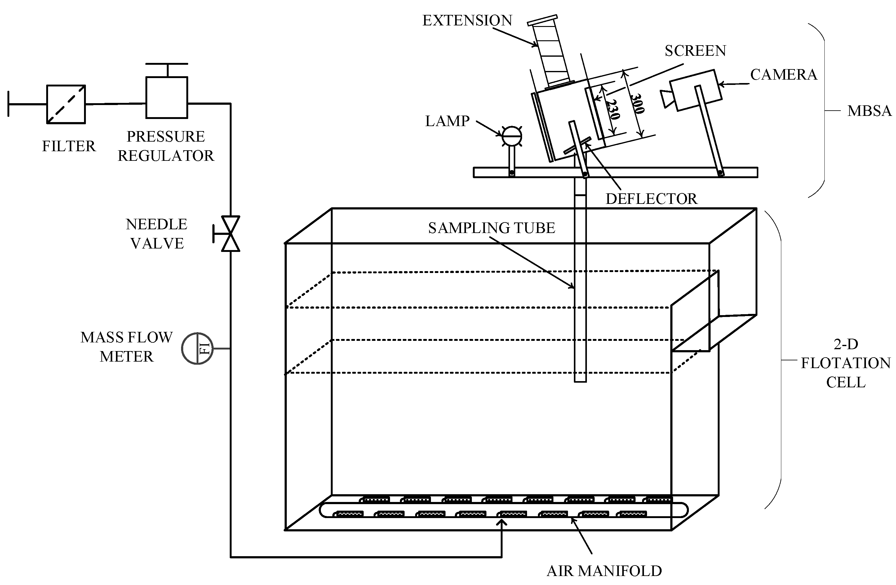
2.1. Experimental Procedure

Bubble size measurements were conducted in the laboratory-scale flotation cell depicted in Figure 1. This 2D cell emulated a slice of an industrial machine with a 140 × 140 cm cross-section and a width of 15 cm. The forced air was controlled and fed from 24 porous spargers. A McGill bubble size analyzer (MBSA) [6] was used for bubble sampling and image recording. This device was initially filled with conditioned water at the same surfactant concentration as in the flotation cell. The rising bubbles were then photographed in a 2D plane with a digital video camera (version, Teledyne Dalsa, Waterloo, ON, Canada), at a sampling rate of one frame per second. All measurements were conducted for 3 minutes at a resolution of 0.056 mm/pxl.

Four types of frothers were studied: methyl isobutyl carbinol (MIBC), AeroFroth^® 70 (Cytec, Woodland Park, NJ, USA), OrePrep^® F-507 (Cytec, Woodland Park, NJ, USA), and Flotanol^® 9946 (Clariant Mining Solutions, Louisville, KY, USA). AeroFroth^® 70 contains MIBC and diisobutyl ketone [30], OrePrep^® F-507 contains glycol and other non-hazardous components [30], and Flotanol^® 9946 corresponds to a 2-ethyl hexanol distillation bottom [31]. The experimental data were divided into training and testing datasets.

Table 1. Flotation tests for training.

Type of Frother	Location	Frother Concentrations, ppm	Superficial Gas Rate, cm/s
MIBC	1 and 2	0, 2, 4, 8, 16	0.5, 1.0, 1.5, 2.0, 2.5
AeroFroth® 70	1	0, 2, 4, 8, 16, 32	0.4, 1.2, 2.0
OrePrep® F-507	1	0, 2, 4, 8, 16, 32	0.4, 1.2, 2.0
Flotanol® 9946	1	0, 2, 4, 8, 16, 32	0.4, 1.2, 2.0

and

Table 2. Flotation tests for testing.

Type of Frother	Location	Frother Concentrations, ppm	Superficial Gas Rate, cm/s
AeroFroth® 70	2	0, 2, 4, 8, 16, 32	0.8, 1.6
		0, 2, 8, 32	0.4, 1.2, 2.0
OrePrep® F-507	2	0, 2, 4, 8, 16, 32	0.8, 1.6
		0, 2, 8, 32	0.4, 1.2, 2.0
Flotanol® 9946	2	0, 2, 4, 8, 16, 32	0.8, 1.6
		0, 2, 8, 32	0.4, 1.2, 2.0

present all the evaluated experimental conditions, including the distribution of the training and testing datasets. Frother concentrations of 0, 2, 4, 8, and 16 ppm were evaluated for all types of frothers, whereas 32 ppm was also assessed for AeroFroth^® 70, OrePrep^® F-507, and Flotanol^® 9946. The superficial gas rates were set to 0.5, 1.0, 1.5, 2.0, and 2.5 cm/s for MIBC, and to 0.4, 0.8, 1.2, 1.6, and 2.0 cm/s for the rest of the frothers. Conditions with high J_G and low concentrations of MIBC favored the transition toward a churn-turbulent regime from an ellipsoidal regime, which was detected in the analysis. All tests were conducted at two locations in the flotation cell. From Table 1 and Table 2, 104 experimental conditions were used in the training procedure and 72 for testing.

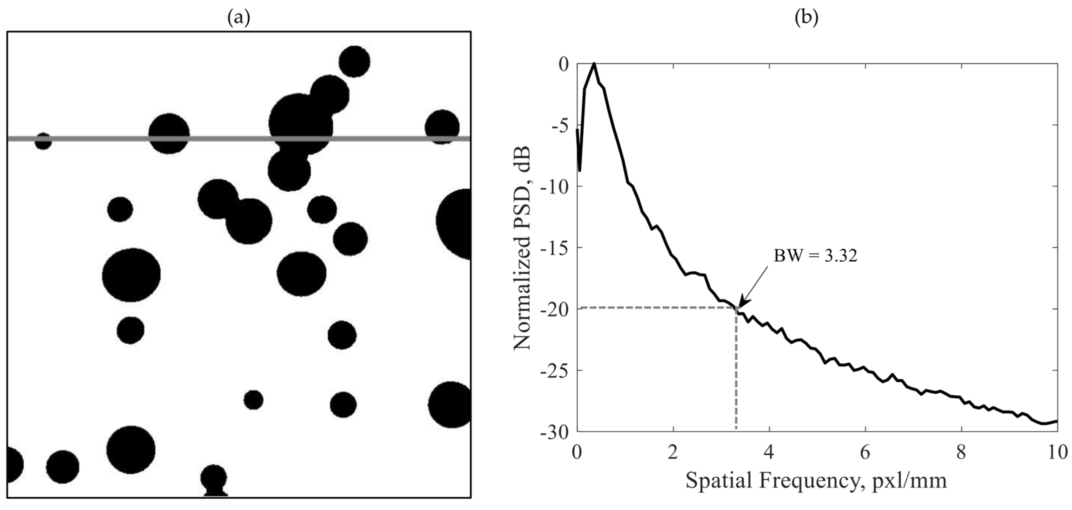
2.2. Semiautomated Image Processing

The BSDs and Sauter mean diameters used as reference (ground truth) were obtained by a semiautomated application based on the Image Processing Toolbox of MATLAB (11.4, The MathWorks Inc., Natick, MA, USA). A field of view of 45 × 35 mm was chosen for image analysis. The images were firstly converted to their binary representation. Bubbles observed as isolated spheres and ellipsoids were identified based on solidity [26]. Objects that presented low solidity were first segmented using Watershed, followed by Hough transforms [13,32]. The previous automated steps were complemented by manual processing: (i) false positives obtained in the automated processing were corrected; (ii) non-identified bubbles (bubbles in clusters and irregular bubbles) were manually estimated. This procedure avoided the biases caused by removing bubbles from the analysis as reported in the literature [13,14,15]. The size of each identified bubble was estimated as an equivalent ellipsoid diameter. The D₃₂ values obtained from the semiautomated algorithm were used as references to evaluate the ability to predict bubble size. We recorded 180 images per experimental condition, from which a subset was randomly chosen to process a minimum of 1500 bubbles per test. However, at least 10 images were processed in all cases. This limit for the number of processed images was especially defined for conditions with a high gas hold-up. All images were analyzed when operating the cell with no frother. For further details on the semiautomated procedure, please refer to Vinnett, Urriola, Orellana, Guajardo and Esteban [29]. Appendix A presents examples of the bubble size distributions obtained by the semiautomated approach.

2.3. Region Properties and Their Association with Bubble Size

The same images that were processed by the semiautomated algorithm were studied in terms of their region properties from their binary representation. The statistical parameters of these properties were analyzed based on their association with the Sauter mean diameter of the BSDs. For example, for the binary image shown in Figure 2a, the object and region properties summarized in

Table 3. List of studied region and object properties.

Property	Variable Symbol	Statistical Index
Shadow Fraction	SF	Median Relative Standard Deviation Relative Interdecile Range Relative Interquintile Range Relative Interquartile Range
$\mathrm{Circularity},4\pi area/P^2$	C
Aspect Ratio, major axis length/minor axis length	AR
Eccentricity	E
Perimeter, mm	P
Solidity	S
$\mathrm{Equivalent}\mathrm{Diameter},\sqrt{4 area/\pi }$, mm	ED
Number of Objects per mm2, 1/mm2	N
Spatial Bandwidth, pxl/mm	BW

were calculated. For each experimental condition and all processed images, the statistics of the properties of all objects (e.g., circularity, solidity, aspect ratio, and perimeter) were estimated to obtain the median and some indicators of variability. In addition, the shadow fraction (black region with respect to the region of interest) and the spatial bandwidth were obtained for each image. The spatial bandwidth was an indicator of the average pulse width generated by the black pixels associated with the bubbles (i.e., disturbances of bubbles over the gray line in Figure 2a). This bandwidth was obtained at −20 dB with respect to the peak in the power spectral density, as shown in Figure 2b [26]. The shadow fraction and the spatial bandwidth have been proven to be correlated with D₃₂ [25,26]. Most of the object features were directly obtained from the Image Processing Toolbox of MATLAB (11.4, The MathWorks Inc., Natick, MA, USA). Circularities, aspect ratios, eccentricities, perimeters, solidities, equivalent diameters, and the number of objects were obtained from the regrionprops function of this toolbox. The estimations of the shadow fractions and spatial bandwidths have been proven to be straightforward, as reported by Vinnett and Alvarez-Silva [25] and Vinnett, Sovechles, Gomez and Waters [26]. Table 3 also presents the variable symbols for each studied feature. The computations of all region and object properties were limited by the bandwidth estimations, whose processing times were proven to be shorter than those of conventional image analysis [26]. The median (subscript 50) along with variability indexes were correlated with D₃₂. Variability was evaluated by the relative standard deviation (subscript RSD), relative interdecile range (subscript RIDR), relative interquintile range (subscript RIQQR), and relative interquartile range (subscript RIQR). Only one variability indicator was used per feature, which was chosen based on the highest level of association with the D₃₂ values.

All properties were related to the measured D₃₂ values using the Pearson coefficient of correlation (R) and the maximal information coefficient [33]. The former measures linear correlation, whereas the latter indicates the level of association between the evaluated variables, not constrained to linear relationships [33]. The maximal information coefficient (MIC) was used to detect variables that were non-linearly related to the Sauter diameter and did not lead to a high coefficient of correlation.

It should be noted that the experimental conditions with no frother and J_G = 0.4, 1.2, and 2.0 cm/s were run six times in different locations of the flotation cell. Manual processing for these three conditions was conducted by 4, 3, and 3 different users, respectively. The relative standard deviations of the estimated D₃₂ were 6.2%, 3.7%, and 2.8%, respectively. These variabilities included the experimental and spatial variability, and uncertainties in the manual processing. The latter was considered acceptable for the purpose of this study.

3. Results

All analyzed region and object properties shown in Table 3 were related to the measured Sauter diameters using the Pearson coefficient of correlation and the maximal information coefficient. Only the training datasets were included in this analysis.

Table 4. Twelve properties that led to the highest coefficients of correlation with D₃₂.

Title	P50	SFRIQQR	ED50	NRSD	BW50	EC50	ARRSD	C50	ECRIDR	N50	AR50	BWRSD
R	0.838	0.831	0.829	0.822	−0.820	0.766	0.762	−0.750	−0.730	−0.717	0.700	0.650
MIC	0.942	0.794	0.960	0.859	1.000	0.813	0.969	0.754	0.798	0.953	0.813	0.477

shows the 12 predictors with the most significant (absolute) coefficients of correlation. From these results, the highest absolute coefficients of correlation did not consistently agree with the highest MICs because the latter were able to detect non-linear associations. Figure 3 presents examples of correlations between some region or image properties and the Sauter diameter of the BSDs. Figure 3a,c illustrate the increasing trends between predictors (relative interquintile range for the shadow fraction and perimeter median) and D₃₂. Except for the variability, which is higher at high D₃₂, these trends are compatible with linear dependencies. The coefficients of correlation between these predictors and D₃₂ thus resulted in higher values compared with other trends. The maximal information coefficients were also high or moderately high for these trends. Figure 3b,d present non-linear trends between the spatial bandwidth and the number of objects per unit area, and D₃₂, respectively. Although clear relationships were observed, the coefficients of correlation resulted in lower values with respect to Figure 3a,b. The maximal information coefficient was therefore effective in determining non-linear associations between the predictors and the Sauter diameter. It should be noted that D₃₂ values greater than 6.0 mm were observed, which were mainly associated with experimental conditions under high superficial gas rates and with MIBC as a frother. These experimental conditions transitioned to churn-turbulent regimes, as exemplified in Appendix B.

The results from Table 4 and Figure 3 show that different fractions of the D₃₂ variability can be explained by the variability of some region and object properties. A multivariable linear model was implemented to obtain the Sauter diameter from all studied predictors. This model was obtained from the training datasets. Predictors that had non-linear trends in relation to D₃₂ were transformed to favor linearity, which was applied to BW₅₀ (Figure 3b), BW_SRSD, and N₅₀ (Figure 3d). Thus, 1/BW₅₀, 1/N₅₀, and ln(BW_SRSD) were employed in the linear regression. The model incorporated a constant term; therefore, 19 parameters were estimated. Robust linear regression was used from the Statistics and Machine Learning toolbox of MATLAB (The MathWorks Inc., Natick, MA, USA). Ordinary least-squares estimation was sensitive to leverage points associated with abnormal gas dispersion conditions, as illustrated in Appendix B. Robust regression performs iteratively reweighted least-squares estimations, assigning a weight to each residual based on its magnitude [34]. This approach was then used to reduce the impact of data points that were far from the main trends. Figure 4 presents the model fitting. A good agreement was observed, except for some tests with D₃₂ > 5.0 mm. According to the procedure reported by Vinnett et al. [35], experimental conditions with relative standard deviations greater than 0.7 in the shadow fraction were removed from the overall dataset, allowing abnormal gas dispersion conditions to be skipped from the analysis.

Five data points were removed from the training dataset. Thus, 99 conditions were used for model fitting. To reduce over-parameterization, ordinary linear regression was conducted using the best-subset approach. All combinations of predictors were used in the model fitting to choose the model structure that led to the lowest predicted residual error sum of squares (PRESS). The PRESS is obtained as the sums of squares of the prediction residuals, after removing one data point at a time. Four predictors were then chosen in the model structure: C₅₀, ED_RIQR, N_RSD and BW₅₀ (reciprocal). The root mean squared error was 0.214 with these four predictors, compared with an RMSE of 0.204 when including all predictors in the regression. Figure 5 shows the model fitting for the training datasets along with the comparisons for the testing datasets. An adequate D₃₂ description was observed for D₃₂ = 1.3–6.7 mm, after removing abnormal gas dispersion conditions. Higher variability was observed for D₃₂ ≥ 4.0 mm, which was caused by the sensitivity of the Sauter diameter to large bubbles. The testing results proved that the model was generalizable to independent datasets. Again, higher dispersion was observed for D₃₂ ≥ 4.0 mm. It should be noted that the modeled D₃₂ values were automatically estimated without individualizing every single bubble. Although the D₃₂ values observed in the 2D cell corresponded to intermediate- and large-size ranges from industrial databases [18,20,36], poorer bubble size estimations are observed for D₃₂ ≥ 2.0 mm by conventional image analysis, as reported by Vinnett, Yianatos, Arismendi and Waters [20]. Thus, the correlation presented here is suitable for ellipsoidal regimes and in the transition toward turbulent regimes. Conventional image analysis (shape factors and object segmentation) is recommended for D₃₂ < 2.0 mm, as no significant bias was observed with this method from industrial data.

Equation (1) presents the D₃₂ model, in which all parameters were significant at the 95% confidence level. All p-values and 95% confidence intervals of the predictors are presented in Appendix C. From Equation (1), a D₃₂ increase is related to variability increases in the number of objects per millimeter square (N_RSD) and in the equivalent diameter (ED_RIQR). The former is caused by the variability in the gas hold-up when transitioning from spherical to ellipsoidal and turbulent conditions [35]. This transition also increased the variability in the equivalent diameter because more irregular bubbles, coexisting with small bubbles, are typically observed at higher D₃₂ values. Lower D₃₂ values were observed at lower median circularities (C₅₀) as small bubbles are consistently observed as spheres in a bubbly regime. As the spatial bandwidth is an indicator of the horizontal and vertical pulse widths that are caused by bubbles (Figure 2a), wider pulses (and lower BW) lead to higher Sauter diameters [26]. A sensitivity analysis proved that BW₅₀ was the most significant predictor. The increases in C₅₀, ED_RIQR, N_RSD, and BW₅₀ from the 25th percentile to the 75th percentile led to D₃₂ variations of −0.13, 0.27, 0.20, and 1.90, respectively. The spatial bandwidth was previously tested with industrial data, adequately explaining the D₃₂ variability for D₃₂ ≈ 2.0–6.0 mm, under normal gas dispersion conditions. Vinnett, Sovechles, Gomez and Waters [26] proposed D₃₂ = α/BW^β to estimate bubble size, obtaining α = 3.7 and β = 1.1 by non-linear regression. As the linear model proposed here incorporates the bandwidth by its reciprocal (β = 1.0), any bias in the industrial variability explained by BW will be moderate with respect to the laboratory results in Figure 5 and Equation (1). It should be noted that Equation (1) only allows for the estimation of the Sauter mean diameter; therefore, additional correlations are required to automatically obtain unbiased BSDs.

$$D_{32}=1.14-1.80C_{50}+0.785E{D}_{\mathrm{RIQR}}+1.52N_{\mathrm{RSD}}+\frac{3.49}{B{W}_{50}}$$

(1)

The results from Table 4 and Figure 3, Figure 4 and Figure 5 show that some image properties were linearly or non-linearly correlated with the Sauter mean diameter. Except for abnormal gas dispersion conditions, these image properties proved to be applicable as predictors to automatically estimate bubble size, without individualizing all single bubbles or removing irregular objects. Additional predictors can be incorporated into the model structure to improve its predictability, using cross-validation to control over-parameterization. The modeling strategy presented here can also be extended to different machine learning tools, considering the continuous improvement in the training stage after increasing D₃₂ and image databases. Thus, gas dispersion data from different flotation machines and scales can be incorporated into the algorithms for model generalizations. Further developments are being made to expand D₃₂ estimations using experimental data from different flotation machines, operating conditions, and flotation scales.

4. Conclusions

One hundred and four images and D₃₂ datasets were studied, correlating different image and object properties (from binary representations) with bubble size. All properties were automatically determined, whereas the D₃₂ values were obtained from a semiautomated approach that did not remove bubbles from the analysis. The main results are summarized as follows:

• Several image and object properties showed moderate or strong correlations, linear and non-linear, with the Sauter diameter.
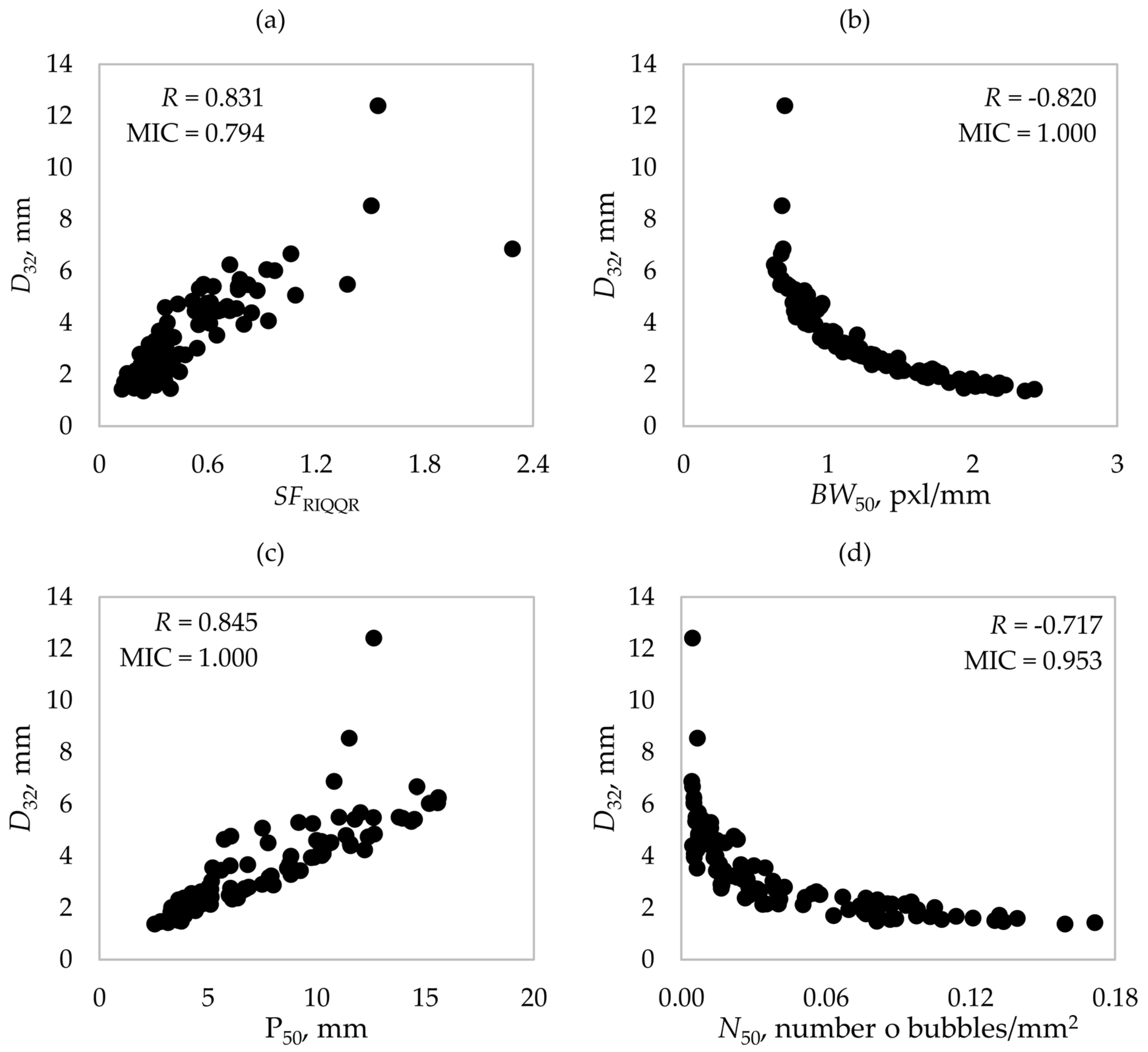
• The maximal information coefficient was successfully used to detect non-linear associations between image and object properties with bubble size. These associations were not clearly detected with the coefficient of correlation. The strongest associations were observed with the median of the spatial bandwidth, median of the equivalent diameter, relative standard deviation of the aspect ratio, and median of the number of objects per unit area.
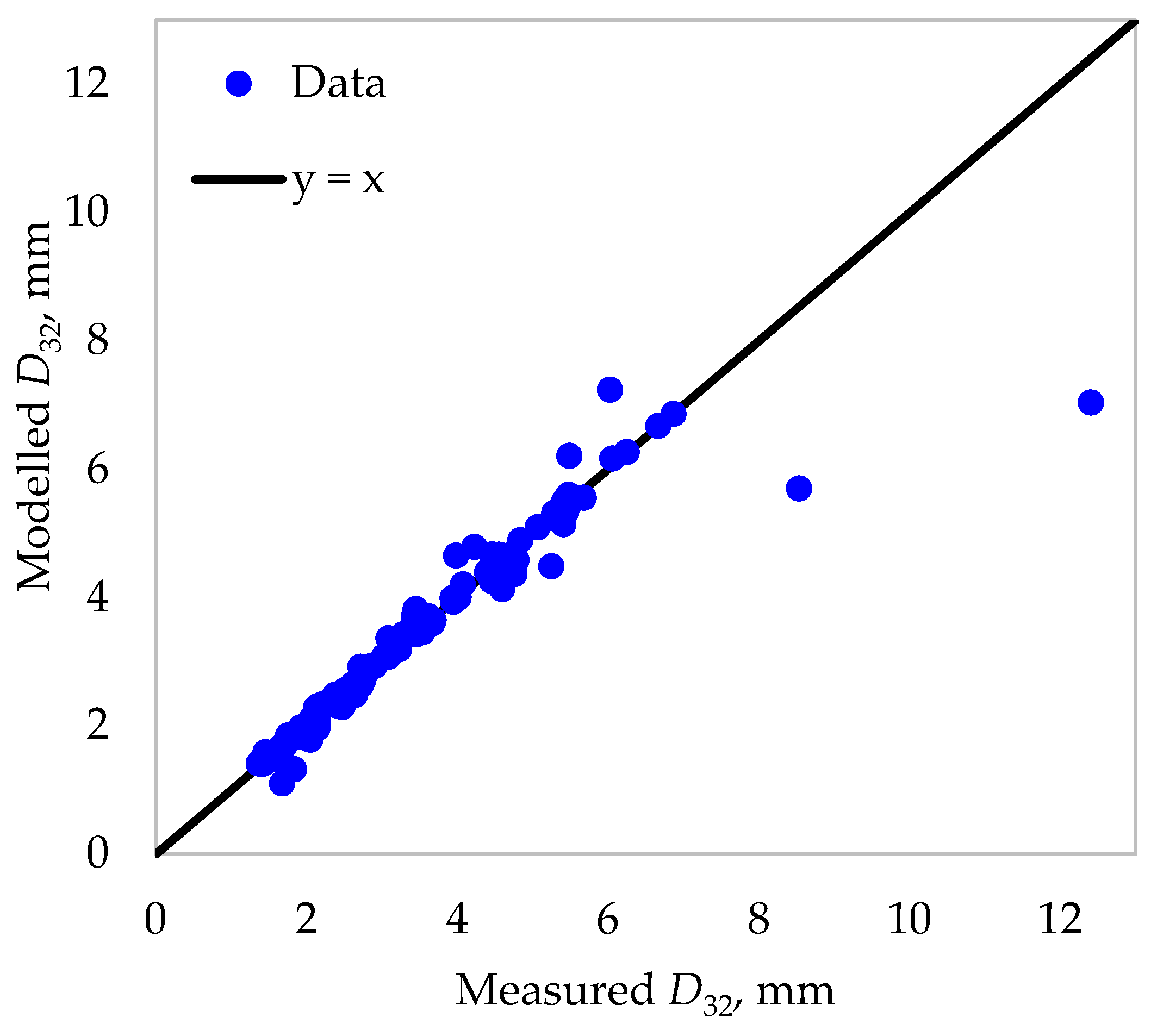
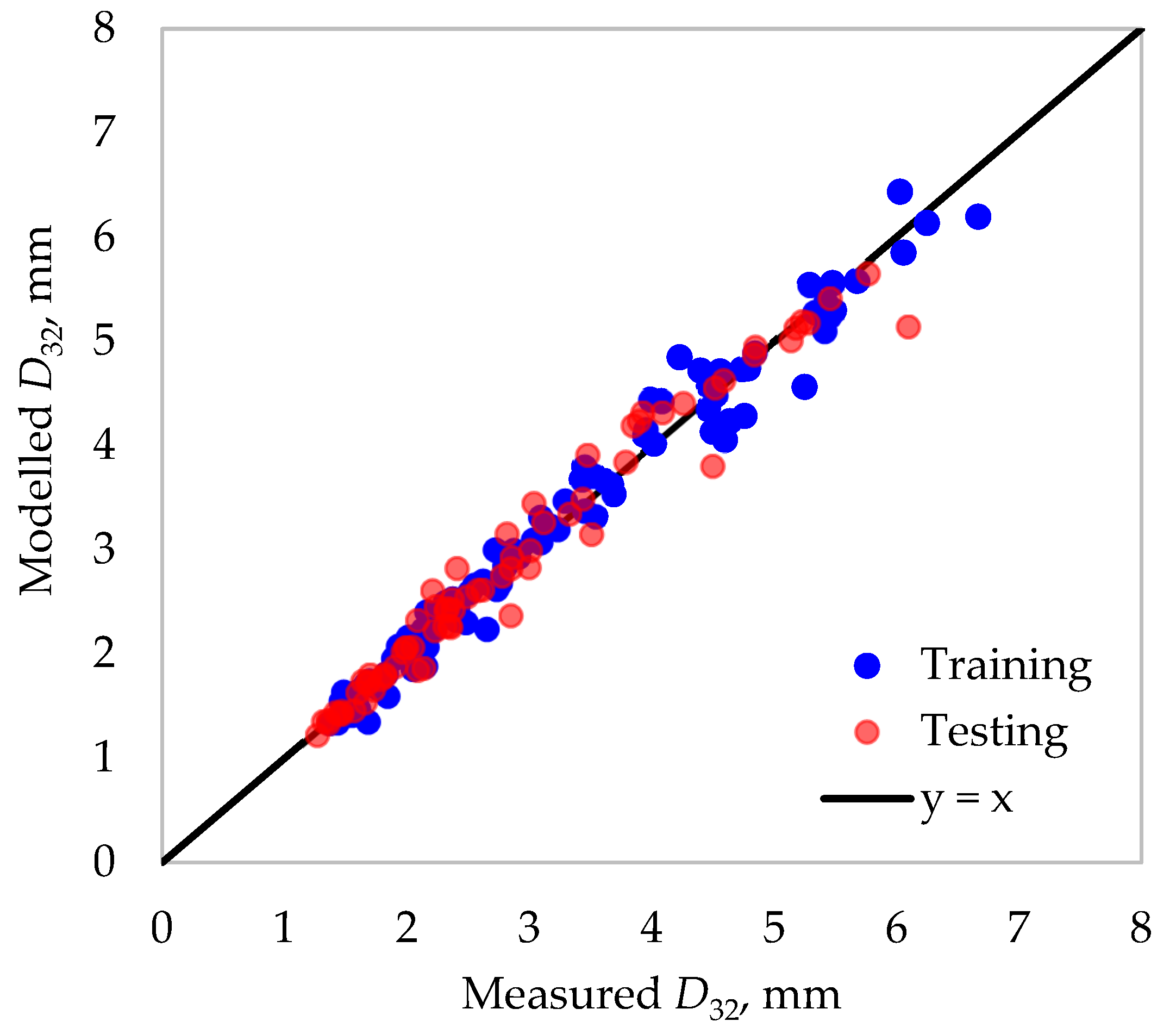
• After removing churn-turbulent conditions and linearizing non-linear associations, a multivariable linear model was proposed, which was able to estimate bubble size in the range 1.3–6.7 mm. This model was obtained from four predictors: median of the circularity, relative interquartile range of the equivalent diameter, relative standard deviation of the number of elements per unit area, and median of the spatial bandwidth. These predictors were chosen from the best subset of all possible linear models, minimizing PRESS.
• The linear model was successfully tested on 72 independent datasets, which showed the generalizability of the model structure.

The strategy to indirectly characterize bubble size from image and object properties proved to be applicable at laboratory scale, without individualizing all single bubbles or removing irregular bubbles and clusters. This approach can be continuously improved by including additional predictors and expanding gas dispersion databases from different experimental conditions.

References

1. Gorain, B.K.; Franzidis, J.P.; Manlapig, E.V. Studies on impeller type, impeller speed and air flow rate in an industrial scale flotation cell. Part 4: Effect of bubble surface area flux on flotation performance. Miner. Eng. 1997, 10, 367–379. [Google Scholar] [CrossRef]
2. Gorain, B.K.; Napier-Munn, T.J.; Franzidis, J.-P.; Manlapig, E.V. Studies on impeller type, impeller speed and air flow rate in an industrial scale flotation cell. Part 5: Validation of k-Sb relationship and effect of froth depth. Miner. Eng. 1998, 11, 615–626. [Google Scholar] [CrossRef]
3. Finch, J.A.; Dobby, G.S. Column Flotation; Pergamon Press: Oxford, UK, 1990. [Google Scholar]
4. Rojas, I.; Vinnett, L.; Yianatos, J.; Iriarte, V. Froth transport characterization in a two-dimensional flotation cell. Miner. Eng. 2014, 66–68, 40–46. [Google Scholar] [CrossRef]
5. Jameson, G.J.; Nam, S.; Young, M.M. Physical factors affecting recovery rates in flotation. Miner. Sci. Eng. 1977, 9, 103–118. [Google Scholar]
6. Hernandez-Aguilar, J.; Gomez, C.; Finch, J. A technique for the direct measurement of bubble size distributions in industrial flotation cells. In Proceedings of the 34th Annual Meeting of the Canadian Mineral Processors, Ottawa, ON, Canada, 22–24 January 2002; pp. 389–402. [Google Scholar]
7. Mesa, D.; Quintanilla, P.; Reyes, F. Bubble Analyser—An open-source software for bubble size measurement using image analysis. Miner. Eng. 2022, 180, 107497. [Google Scholar] [CrossRef]
8. Grau, R.A.; Heiskanen, K. Visual technique for measuring bubble size in flotation machines. Miner. Eng. 2002, 15, 507–513. [Google Scholar] [CrossRef]
9. Acuña, C.; Vinnett, L.; Kuan, S.H. Improving image analysis of online bubble size measurements with enhanced algorithms. In Proceedings of the 12th International Mineral Processing Conference, Procemin, Santiago, Chile, 26–28 October 2016. [Google Scholar]
10. Bailey, M.; Gomez, C.O.; Finch, J.A. Development and application of an image analysis method for wide bubble size distributions. Miner. Eng. 2005, 18, 1214–1221. [Google Scholar] [CrossRef]
11. Sovechles, J.M.; Waters, K.E. Effect of ionic strength on bubble coalescence in inorganic salt and seawater solutions. AIChE J. 2015, 61, 2489–2496. [Google Scholar] [CrossRef]
12. Grau, R.A.; Heiskanen, K. Gas dispersion measurements in a flotation cell. Miner. Eng. 2003, 16, 1081–1089. [Google Scholar] [CrossRef]
13. Riquelme, A.; Desbiens, A.; Bouchard, J.; del Villar, R. Parameterization of Bubble Size Distribution in Flotation Columns. IFAC Proc. Vol. 2013, 46, 128–133. [Google Scholar] [CrossRef]
14. Karn, A.; Ellis, C.; Arndt, R.; Hong, J. An integrative image measurement technique for dense bubbly flows with a wide size distribution. Chem. Eng. Sci. 2015, 122, 240–249. [Google Scholar] [CrossRef]
15. Ma, Y.; Yan, G.; Scheuermann, A.; Bringemeier, D.; Kong, X.-Z.; Li, L. Size distribution measurement for densely binding bubbles via image analysis. Exp. Fluids 2014, 55, 1860. [Google Scholar] [CrossRef]
16. Grau, R.A.; Heiskanen, K. Bubble size distribution in laboratory scale flotation cells. Miner. Eng. 2005, 18, 1164–1172. [Google Scholar] [CrossRef]
17. Lau, Y.M.; Deen, N.G.; Kuipers, J.A.M. Development of an image measurement technique for size distribution in dense bubbly flows. Chem. Eng. Sci. 2013, 94, 20–29. [Google Scholar] [CrossRef]
18. Vinnett, L.; Yianatos, J.; Alvarez-Silva, M. Gas dispersion measurements in industrial flotation equipment. In Proceedings of the 8th Copper International Conference, Copper 2013, Santiago, Chile, 1–4 December 2013. [Google Scholar]
19. Wang, J.; Forbes, G.; Forbes, E. Frother Characterization Using a Novel Bubble Size Measurement Technique. Appl. Sci. 2022, 12, 750. [Google Scholar] [CrossRef]
20. Vinnett, L.; Yianatos, J.; Arismendi, L.; Waters, K.E. Assessment of two automated image processing methods to estimate bubble size in industrial flotation machines. Miner. Eng. 2020, 159, 106636. [Google Scholar] [CrossRef]
21. Steinemann, J.; Buchholz, R. Application of an Electrical Conductivity Microprobe for the Characterization of bubble behavior in gas-liquid bubble flow. Part. Part. Syst. Charact. 1984, 1, 102–107. [Google Scholar] [CrossRef]
22. Meernik, P.; Yuen, M. An optical method for determining bubble size distributions—Part II: Application to bubble size measurement in a three-phase fluidized bed. J. Fluids Eng. 1988, 110, 332–338. [Google Scholar] [CrossRef]
23. Kracht, W.; Emery, X.; Paredes, C. A stochastic approach for measuring bubble size distribution via image analysis. Int. J. Miner. Processing 2013, 121, 6–11. [Google Scholar] [CrossRef]
24. Kracht, W.; Moraga, C. Acoustic measurement of the bubble Sauter mean diameter d32. Miner. Eng. 2016, 98, 122–126. [Google Scholar] [CrossRef]
25. Vinnett, L.; Alvarez-Silva, M. Indirect estimation of bubble size using visual techniques and superficial gas rate. Miner. Eng. 2015, 81, 5–9. [Google Scholar] [CrossRef]
26. Vinnett, L.; Sovechles, J.; Gomez, C.O.; Waters, K.E. An image analysis approach to determine average bubble sizes using one-dimensional Fourier analysis. Miner. Eng. 2018, 126, 160–166. [Google Scholar] [CrossRef]
27. Ilonen, J.; Juránek, R.; Eerola, T.; Lensu, L.; Dubská, M.; Zemčík, P.; Kälviäinen, H. Comparison of bubble detectors and size distribution estimators. Pattern Recognit. Lett. 2018, 101, 60–66. [Google Scholar] [CrossRef]
28. Bu, X.; Zhou, S.; Sun, M.; Alheshibri, M.; Khan, M.S.; Xie, G.; Chelgani, S.C. Exploring the Relationships between Gas Dispersion Parameters and Differential Pressure Fluctuations in a Column Flotation. ACS Omega 2021, 6, 21900–21908. [Google Scholar] [CrossRef]
29. Vinnett, L.; Urriola, B.; Orellana, F.; Guajardo, C.; Esteban, A. Reducing the Presence of Clusters in Bubble Size Measurements for Gas Dispersion Characterizations. Minerals 2022, 12, 1148. [Google Scholar] [CrossRef]
30. Saavedra Moreno, Y.; Bournival, G.; Ata, S. Classification of flotation frothers—A statistical approach. Chem. Eng. Sci. 2022, 248, 117252. [Google Scholar] [CrossRef]
31. Arends, M.A. Reactivos de Flotación: Evaluación de Colectores y Espumantes; Clariant: Muttenz, Switzerland, 2019. [Google Scholar]
32. Grau, R.A. An Investigation of the Effect of Physical and Chemical Variables on Bubble Generation and Coalescence in Laboratory Scale Flotation Cells; Helsinki University of Technology: Helsinki, Finland, 2006. [Google Scholar]
33. Reshef, D.N.; Reshef, Y.A.; Finucane, H.K.; Grossman, S.R.; McVean, G.; Turnbaugh, P.J.; Lander, E.S.; Mitzenmacher, M.; Sabeti, P.C. Detecting novel associations in large data sets. Science 2011, 334, 1518–1524. [Google Scholar] [CrossRef] [Green Version]
34. Holland, P.W.; Welsch, R.E. Robust regression using iteratively reweighted least-squares. Commun. Stat.-Theory Methods 1977, 6, 813–827. [Google Scholar] [CrossRef]
35. Vinnett, L.; Yianatos, J.; Acuña, C.; Cornejo, I. A Method to Detect Abnormal Gas Dispersion Conditions in Flotation Machines. Minerals 2022, 12, 125. [Google Scholar] [CrossRef]
36. Vinnett, L.; Yianatos, J.; Alvarez, M. Gas dispersion measurements in mechanical flotation cells: Industrial experience in Chilean concentrators. Miner. Eng. 2014, 57, 12–15. [Google Scholar] [CrossRef]
Figure 1. Two-dimensional flotation cell and installation of the McGill bubble size analyzer [29].
Minerals 12 01528 g001
Figure 2. (a) Example of binary image, and (b) normalized power spectral density and bandwidth estimation.
Minerals 12 01528 g002
Figure 3. Correlation between different object/image properties and the Sauter diameter: (a) D32 versus SFRIQQR, (b) D32 versus BW50, (c) D32 versus P50, and (d) D32 versus N50.
Minerals 12 01528 g003
Figure 4. Measured versus modelled Sauter diameters: robust linear regression in the presence of churn-turbulent conditions.
Minerals 12 01528 g004
Figure 5. Measured versus modeled Sauter diameters: training and testing datasets, after removing abnormal conditions.
Minerals 12 01528 g005