
Comparison of Fuzzy and Neural Network Computing Techniques for Performance Prediction of an Industrial Copper Flotation Circuit
 ,
,  ,
,
Abstract
:1. Introduction
2. Materials and Methods
2.1. Input and Output Variables
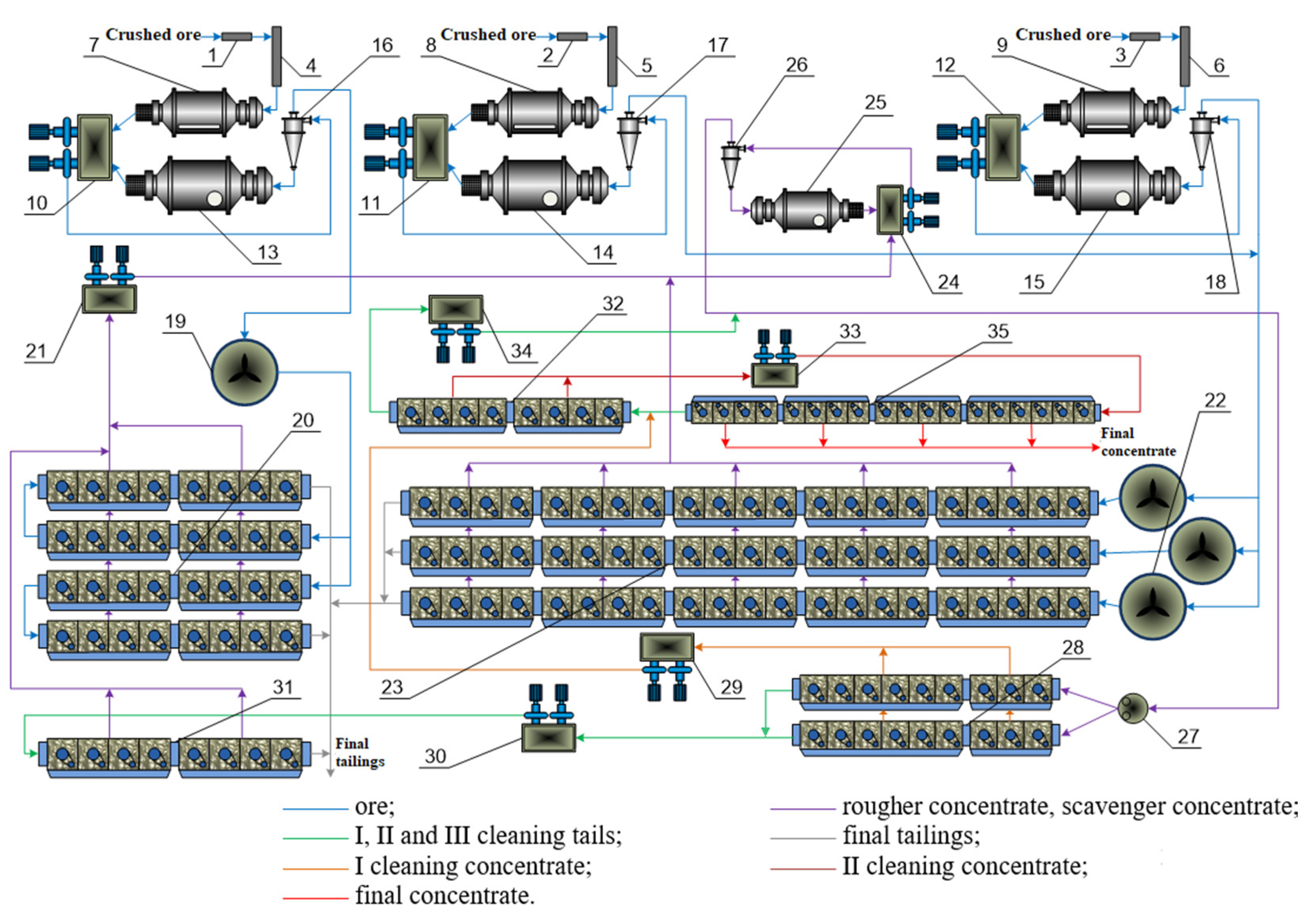
2.1.1. Brief Description of the Veliki Krivelj Flotation Plant
2.1.2. Data Collection
2.1.3. Selection of Variables
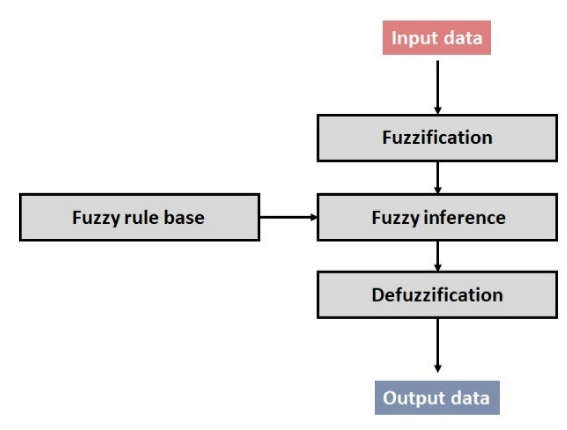
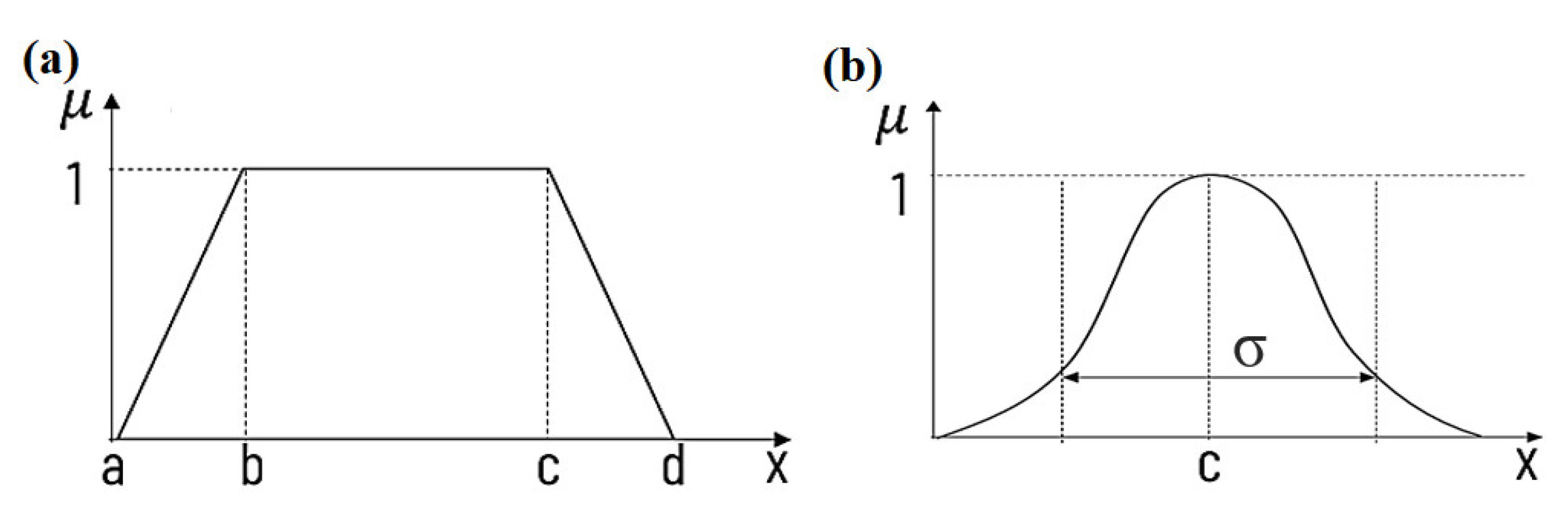
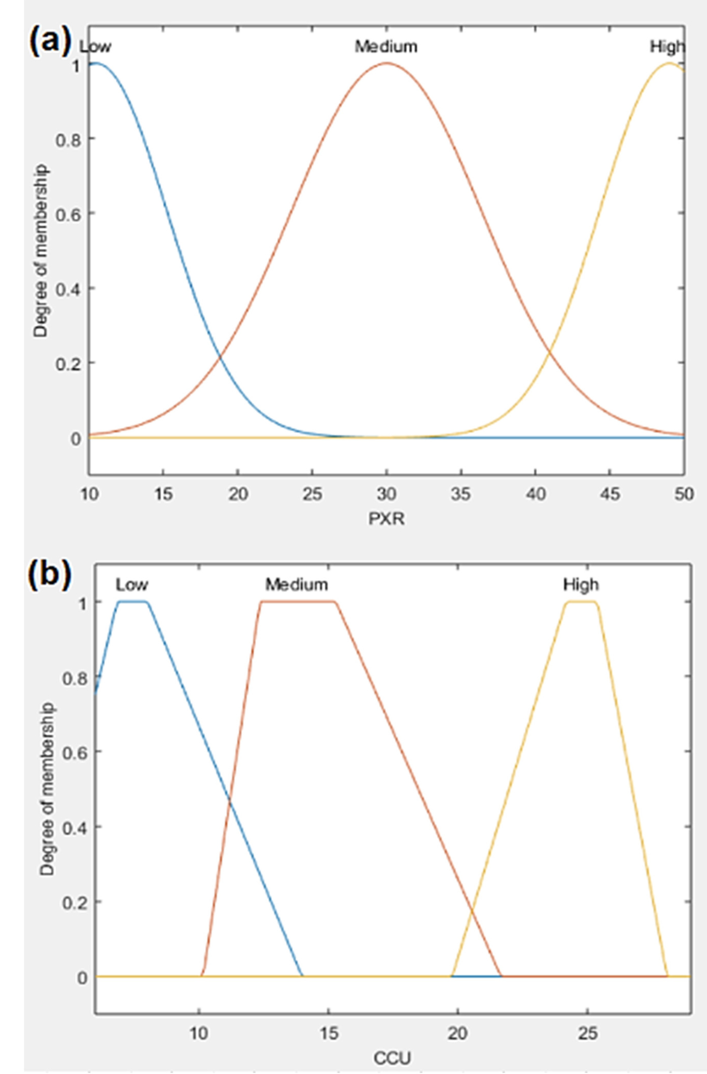
2.2. Methodology of Fuzzy System
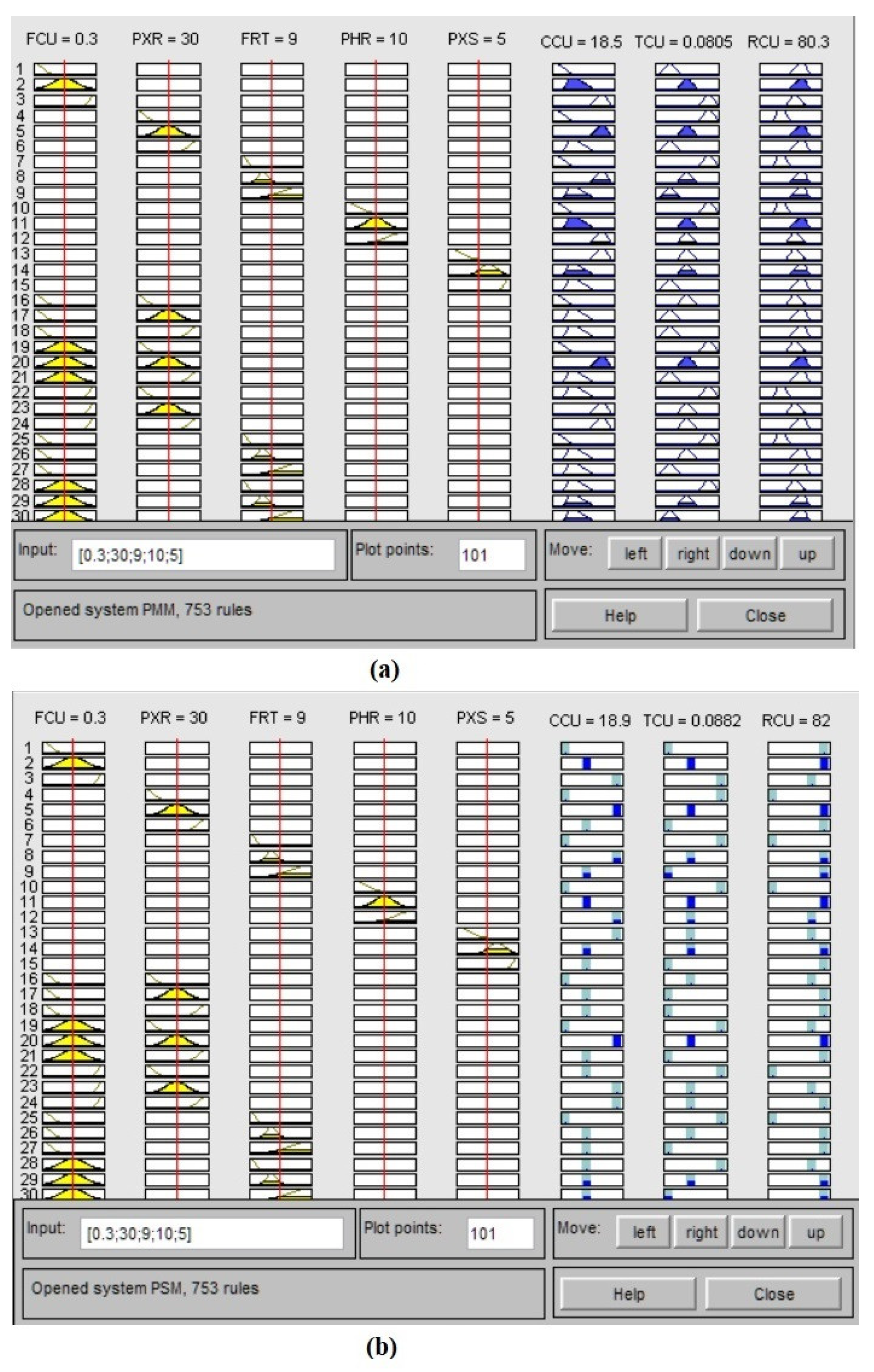
2.2.1. Fuzzy Logic Model Based on Mamdani Inference System—PMM
- Mamdani inference system;
- Applied AND operator in all rules;
- Implication by the minimum method;
- Aggregation by the maximum method; and
- Defuzzification by the centroid method.
- (1)
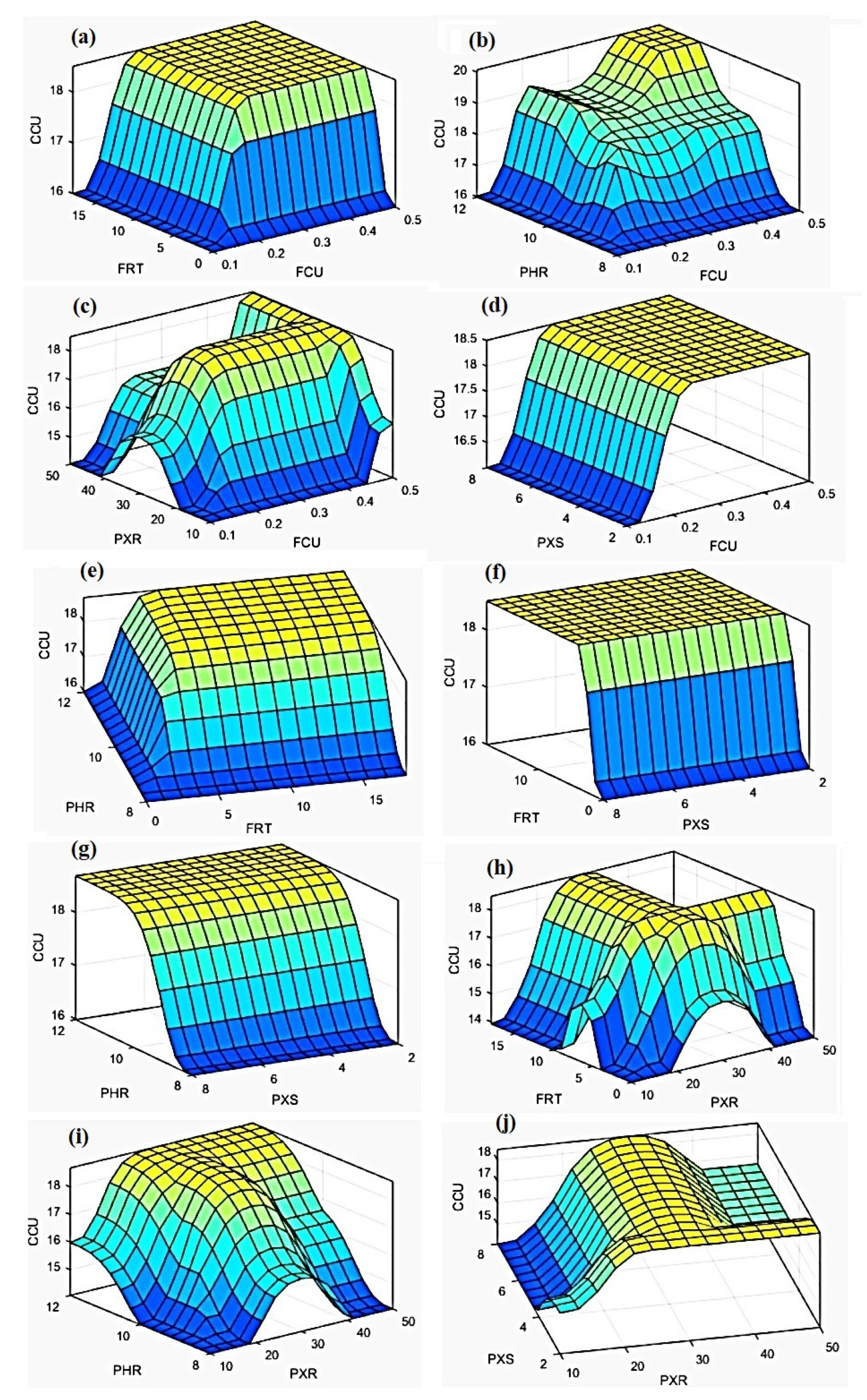
- The surface that shows the dependence of the final concentrate grade (CCU) on copper content in the feed (FCU) and collector consumption at a rougher flotation circuit (PXR), Figure 7c;
- (2)
- The surface that demonstrates dependence of the final grade of tailings (TCU) on the copper content in the feed (FCU) and frother consumption (FRT), Figure 9a.
2.2.2. Fuzzy Logic Model Based on Takagi Sugeno Inference System—PSM
- Takagi-Sugeno inference system; applied AND operator in all rules;
- Implication by the product method;
- Aggregation by the sum method and
- Defuzzification by the weighted average method.
- (1)
- The surface that shows the dependence of the final concentrate grade (CCU) on the copper content in the feed (FCU) and the pulp pH at the rougher circuit (PHR), Figure 10b; and
- (2)
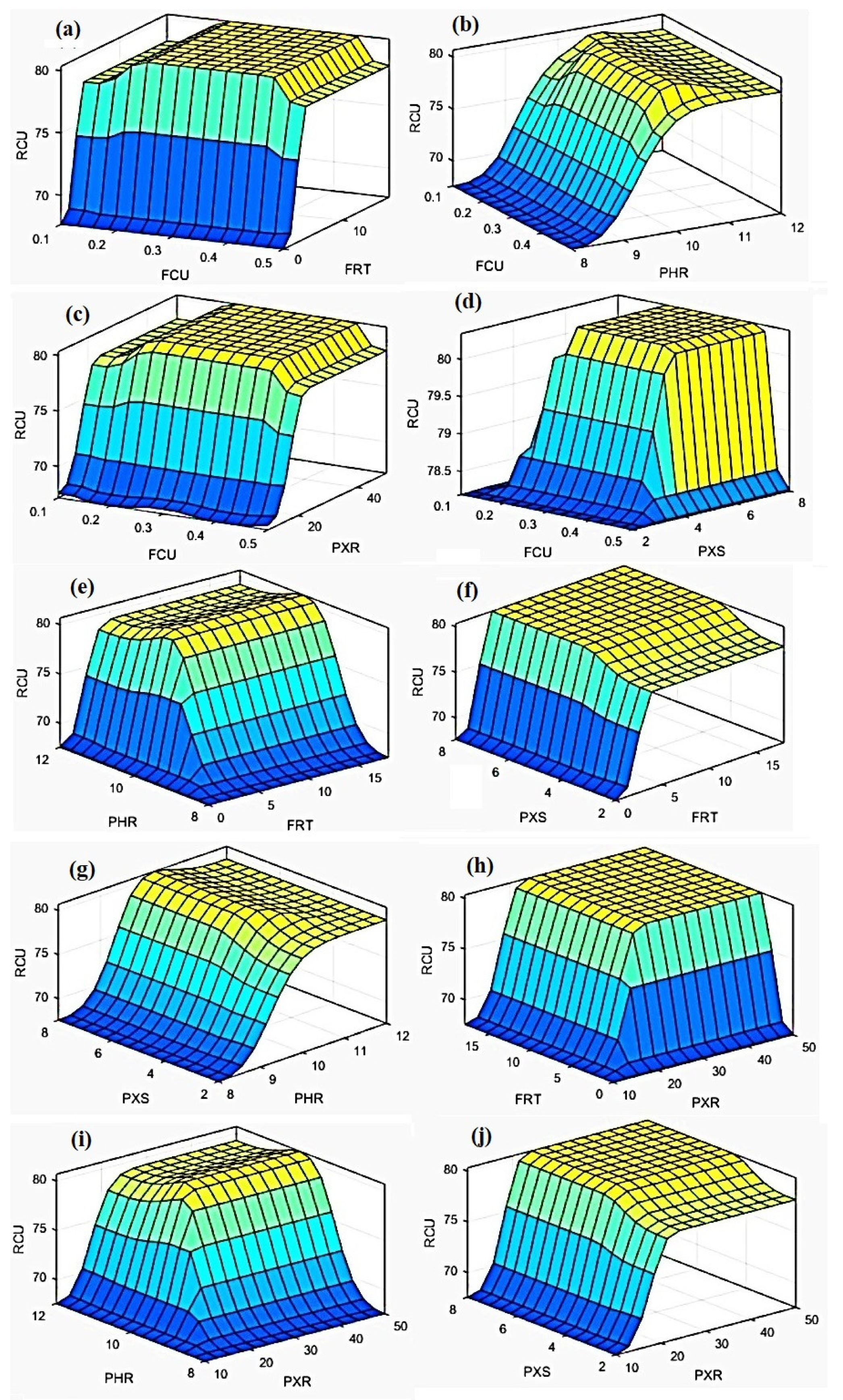
- The surface that displays the dependence of copper recovery in the final concentrate (RCU) on the copper content in the feed (FCU) and the consumption of the collector at the scavenger circuit (PXS), Figure 11d.
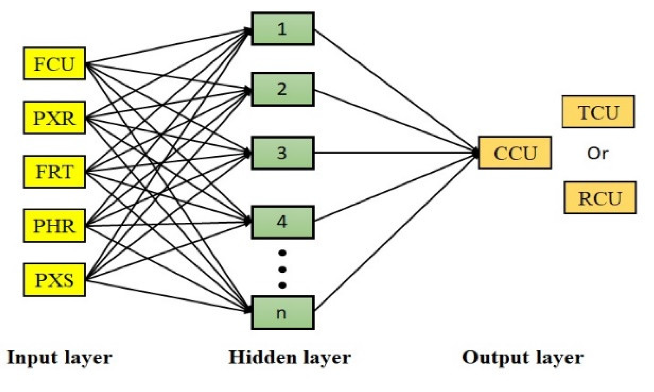
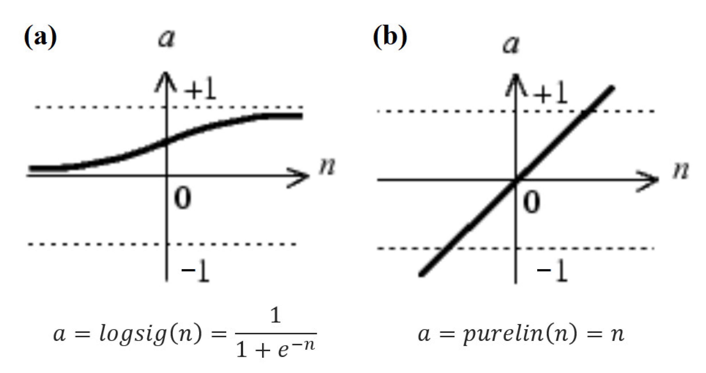
2.3. Artificial Neural Network
3. Results and Discussion
3.1. Performance Evaluation of the Fuzzy Models
3.2. Neural Network-Based Models
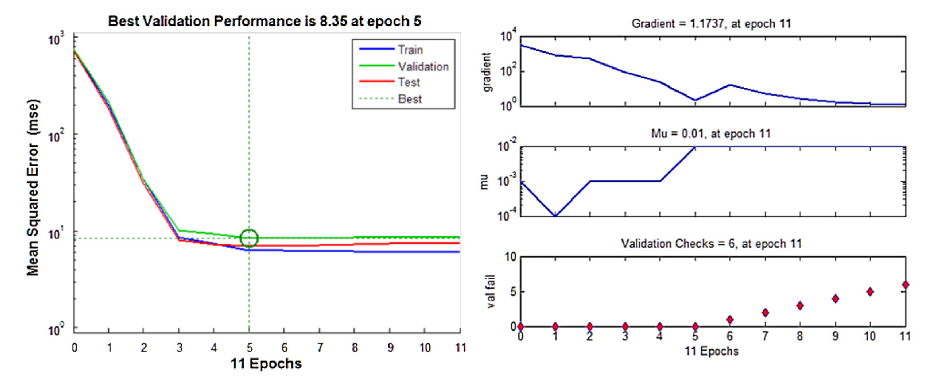
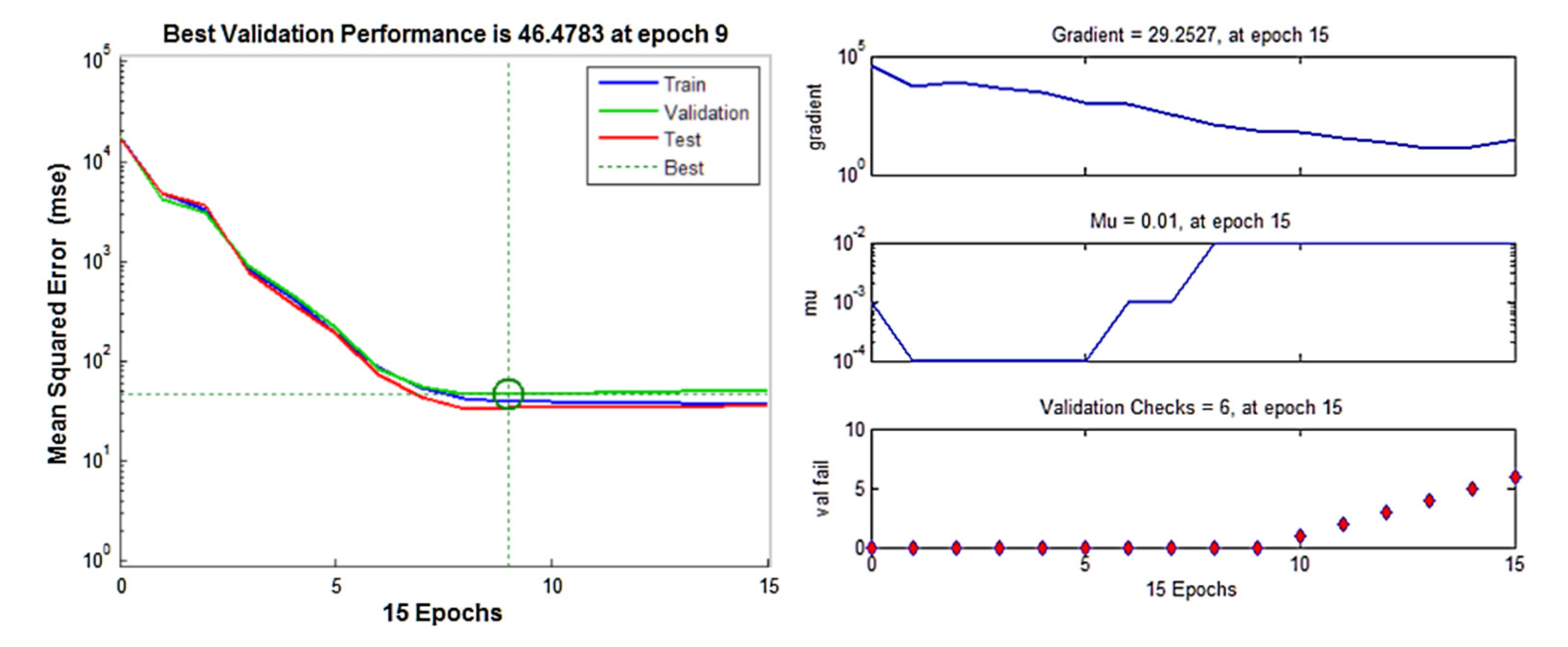
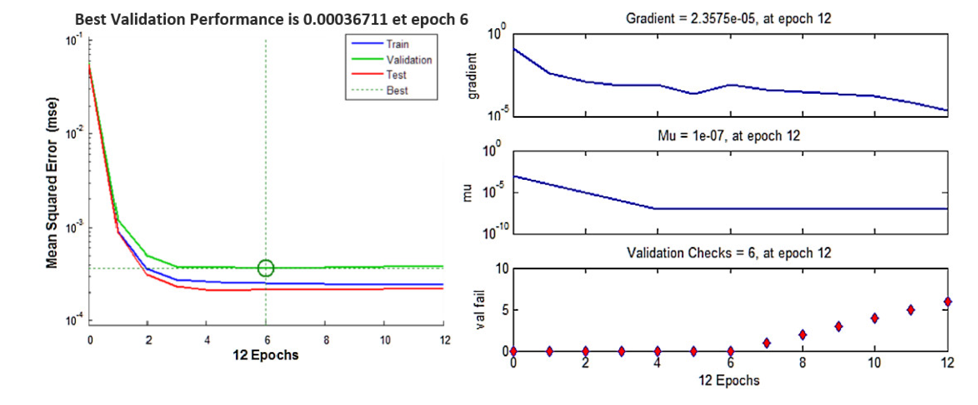
3.2.1. Model Performances
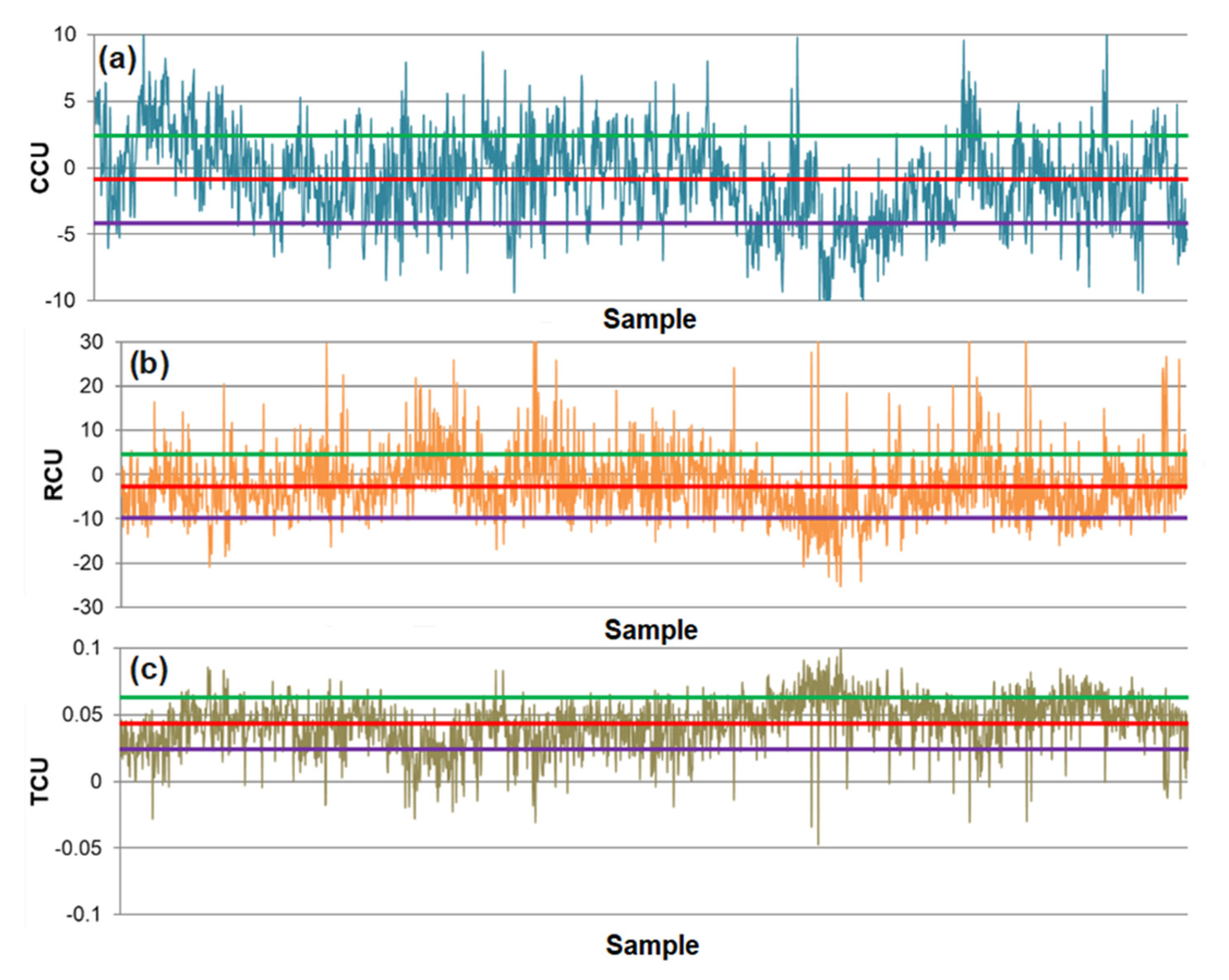
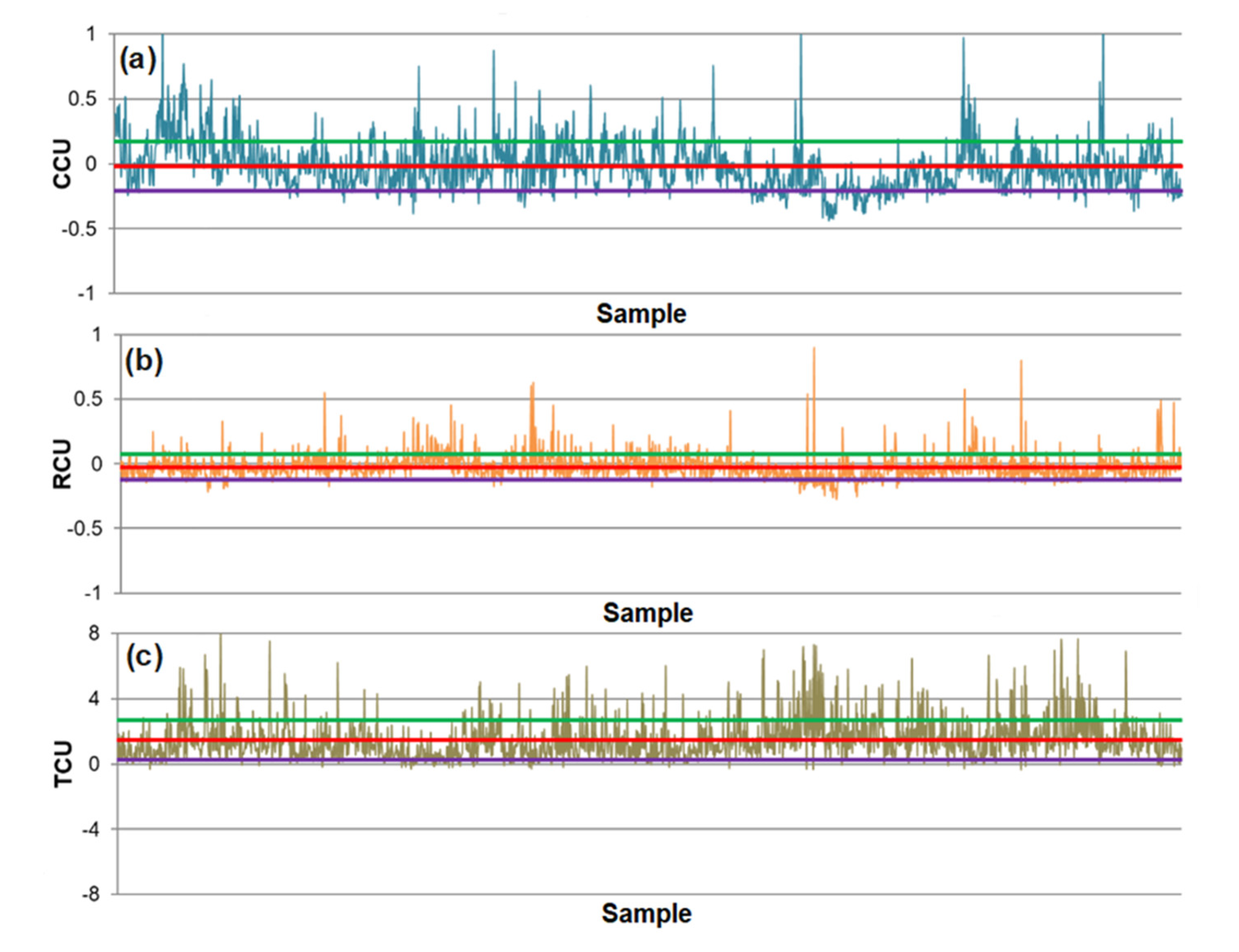
3.2.2. Predictive Abilities of NN-Based Models
3.3. Summary Discussion
4. Conclusions
- The purpose of modeling the production process in the Veliki Krivelj plant is the possibility of implementing the obtained models into an automatic control system of this process. This system would include the application of controllers based on fuzzy logic or artificial neural networks.
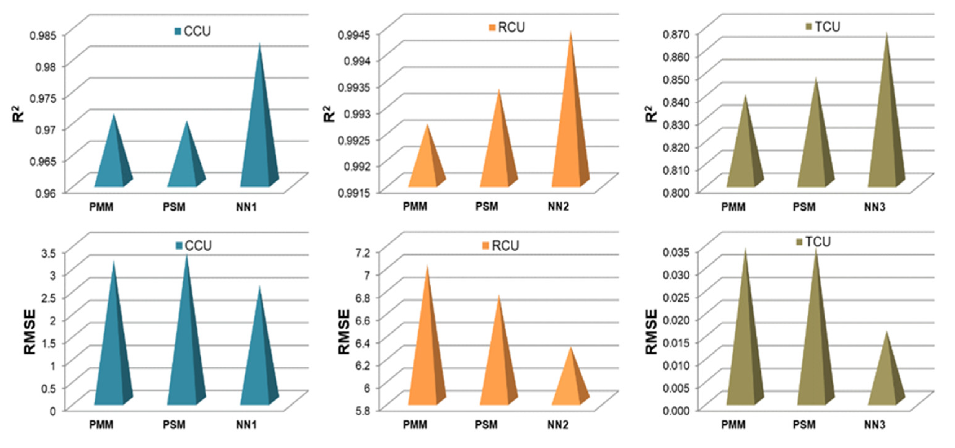
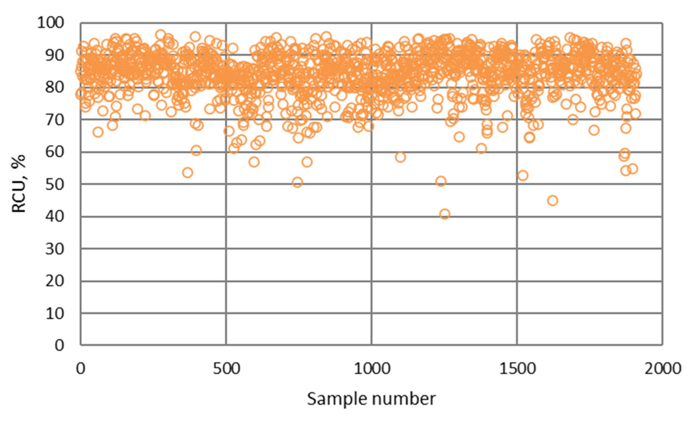
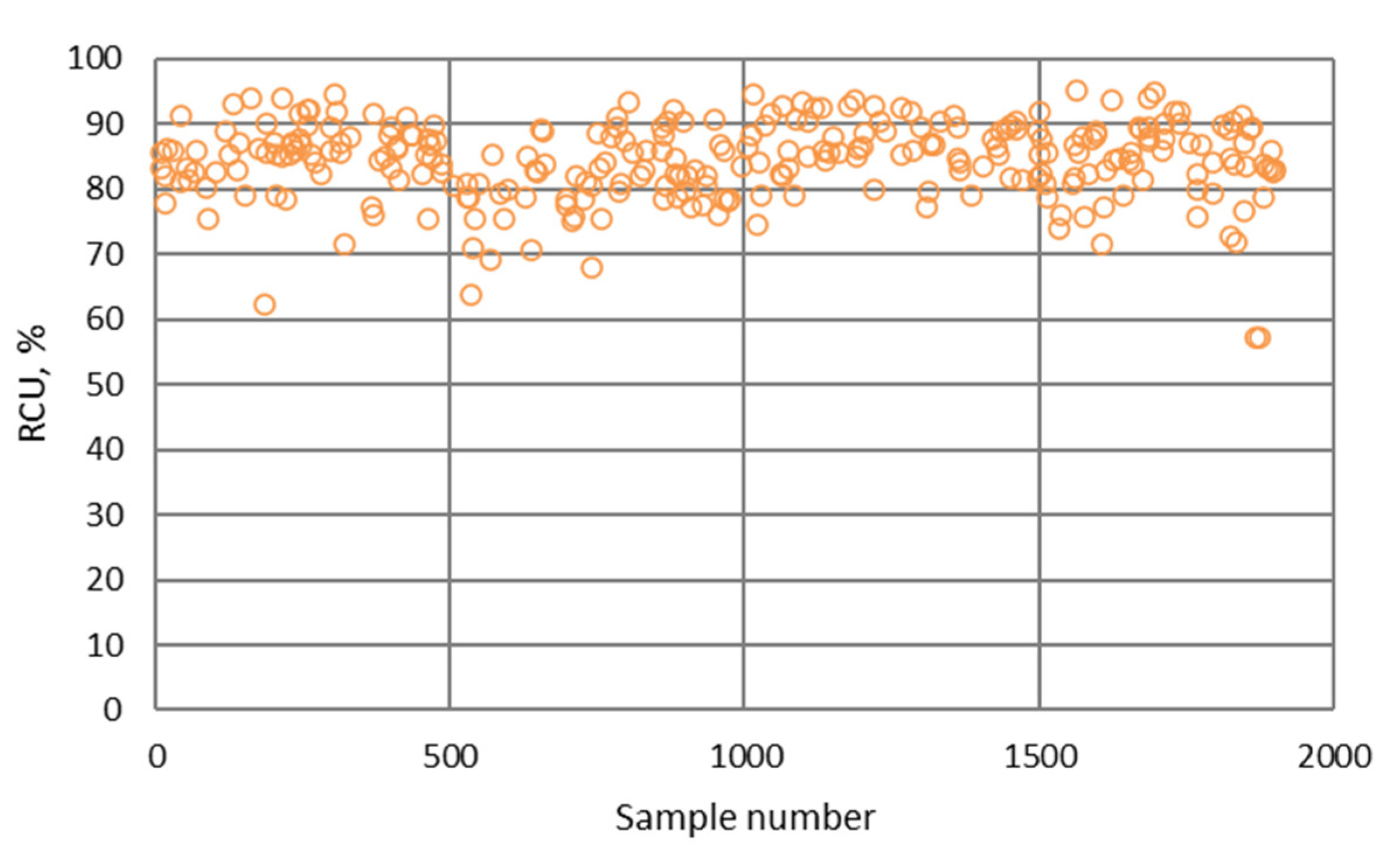
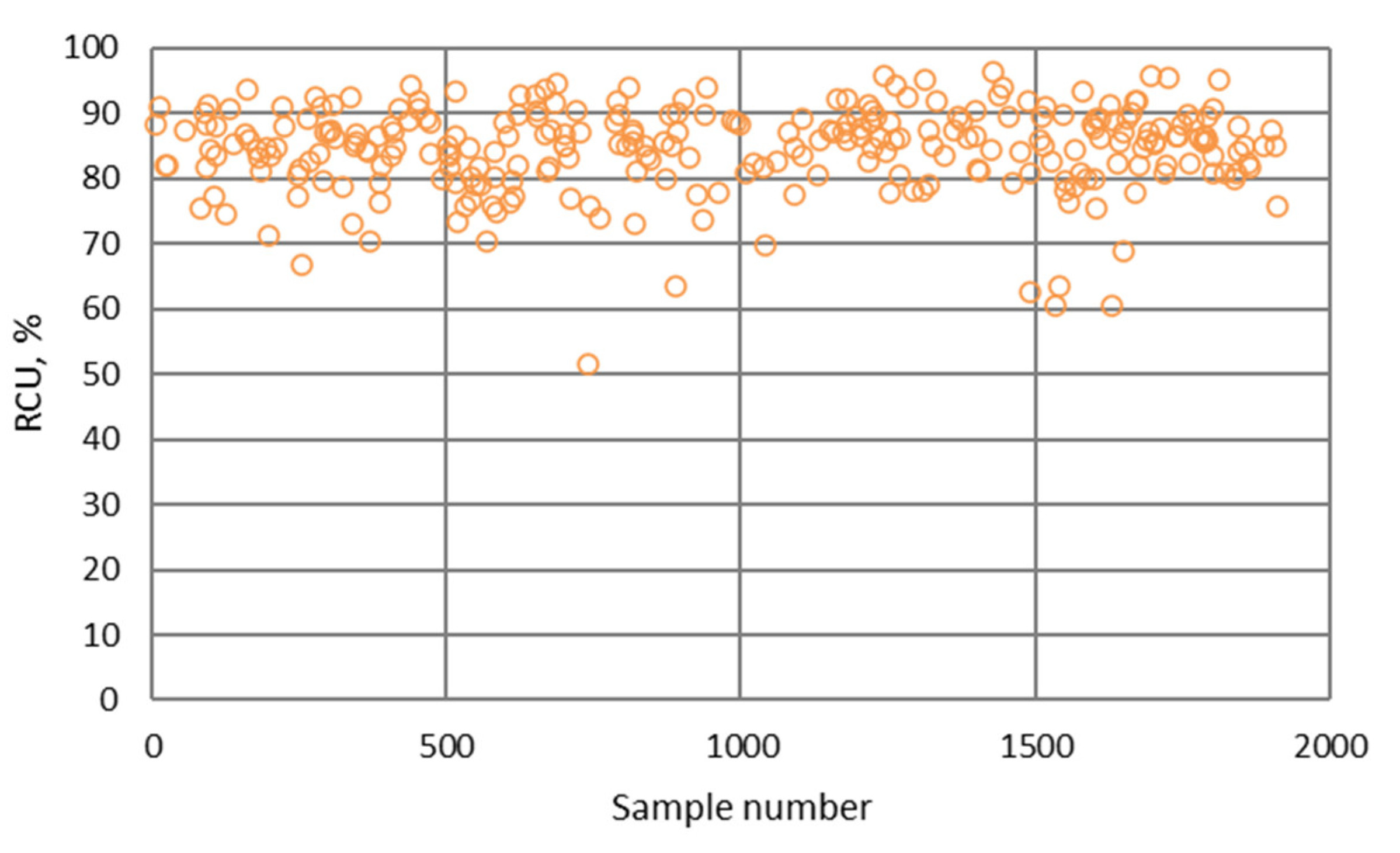
- The NN and fuzzy logic models provided effective estimations due to the high R2 and low RMSE values. However, the NN models were slightly more robust and accurate in predicting the values of metallurgical factors compared to the fuzzy logic models. The RMSE values of the NN models for the prediction of copper grade and recovery of the final concentrate were 2.567 and 6.284, respectively.
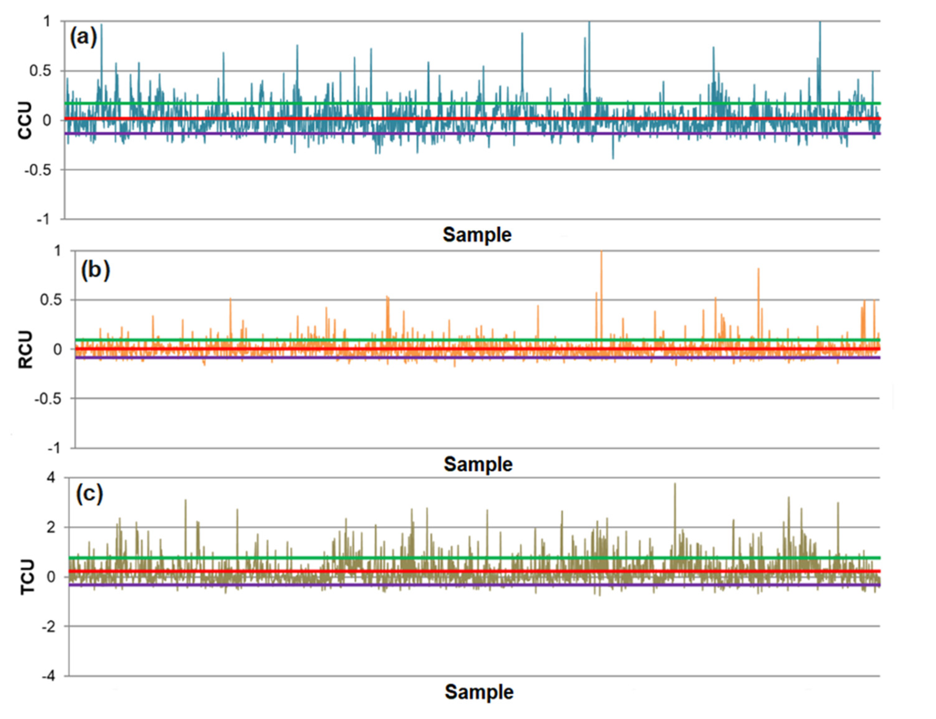
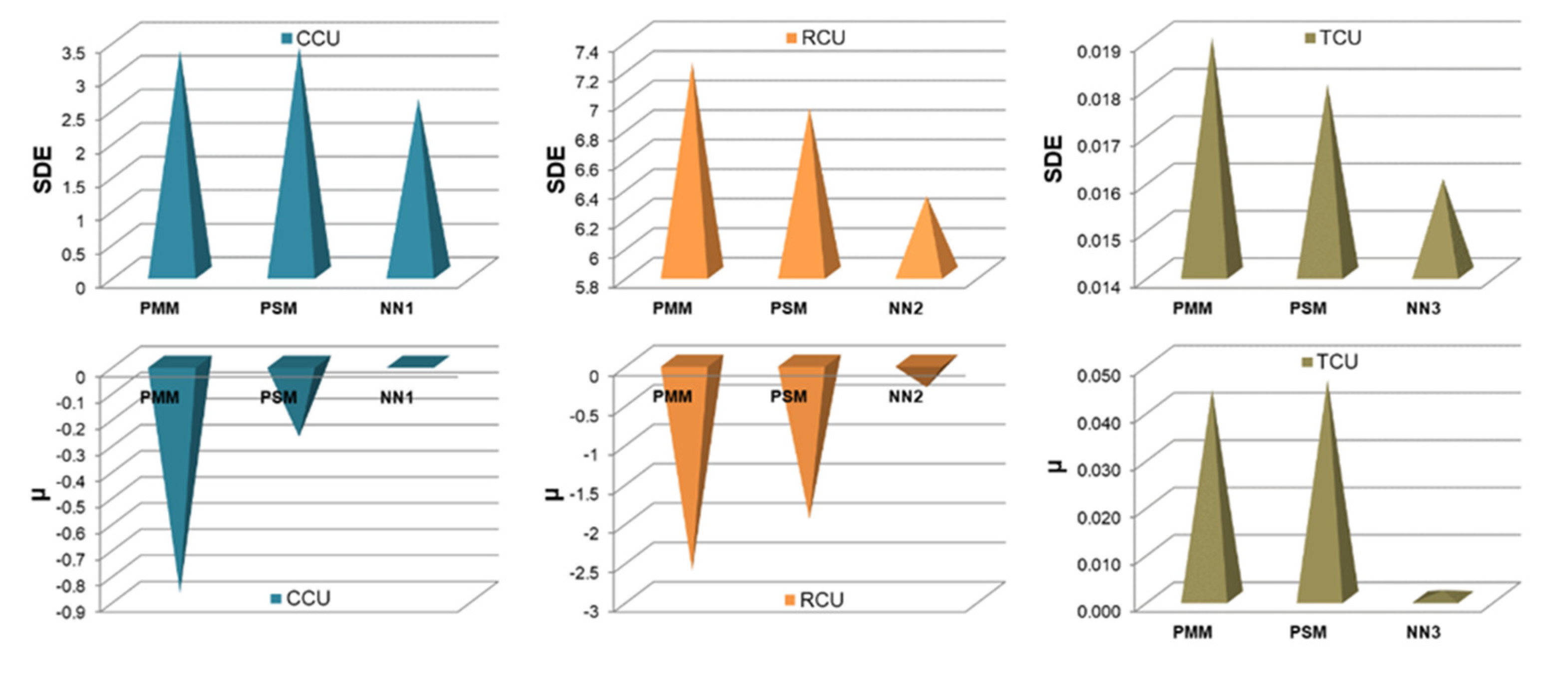
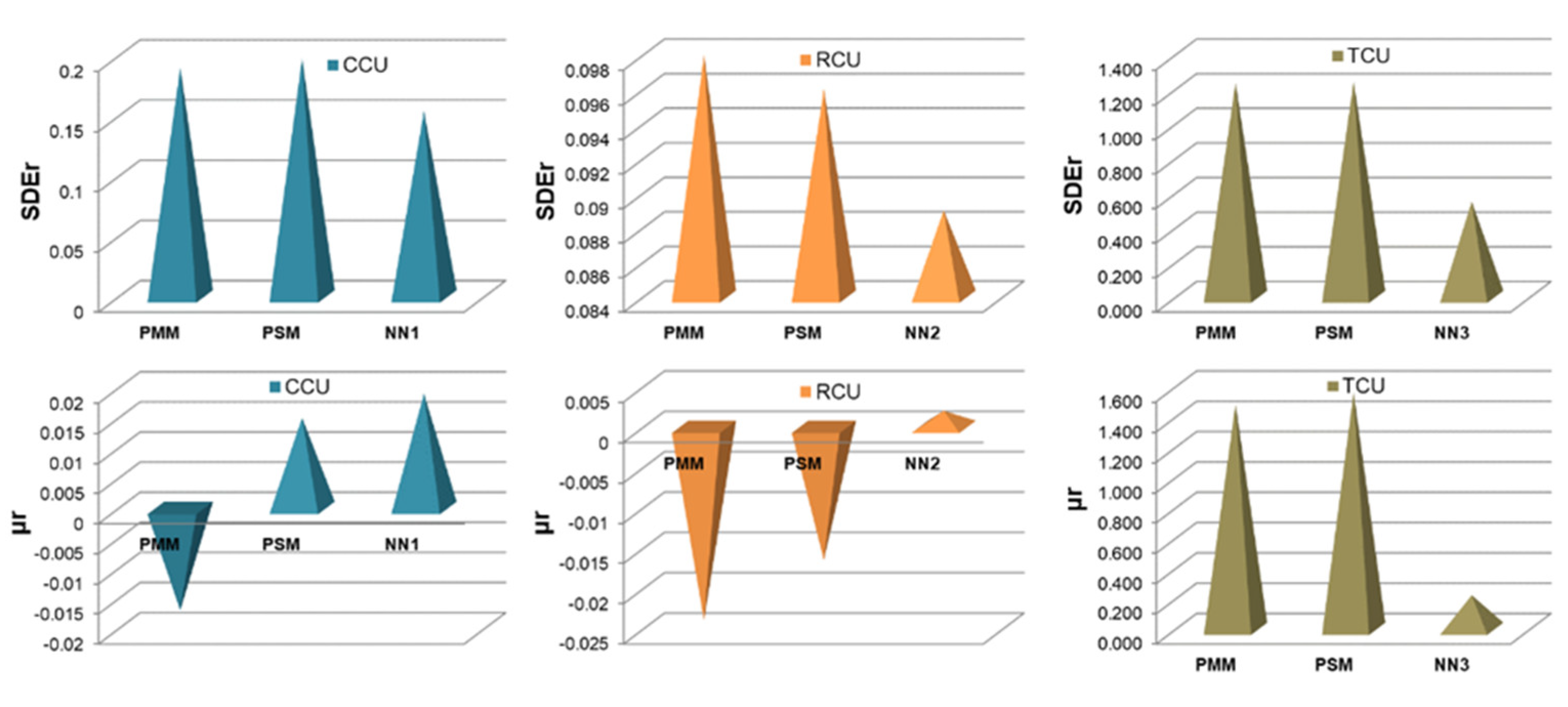
- Neural networks have the smallest standard deviations of the absolute and relative prediction error for all output variables.
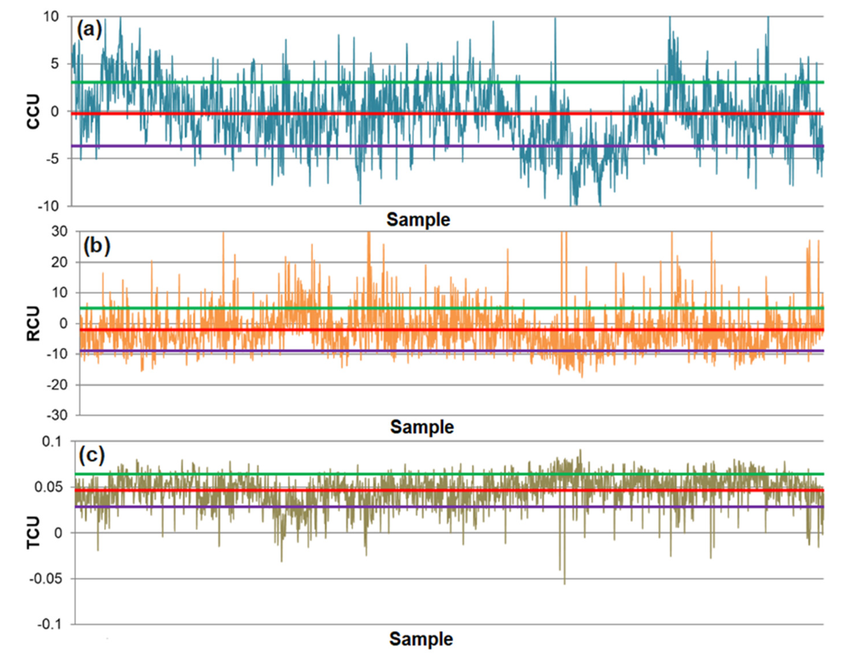
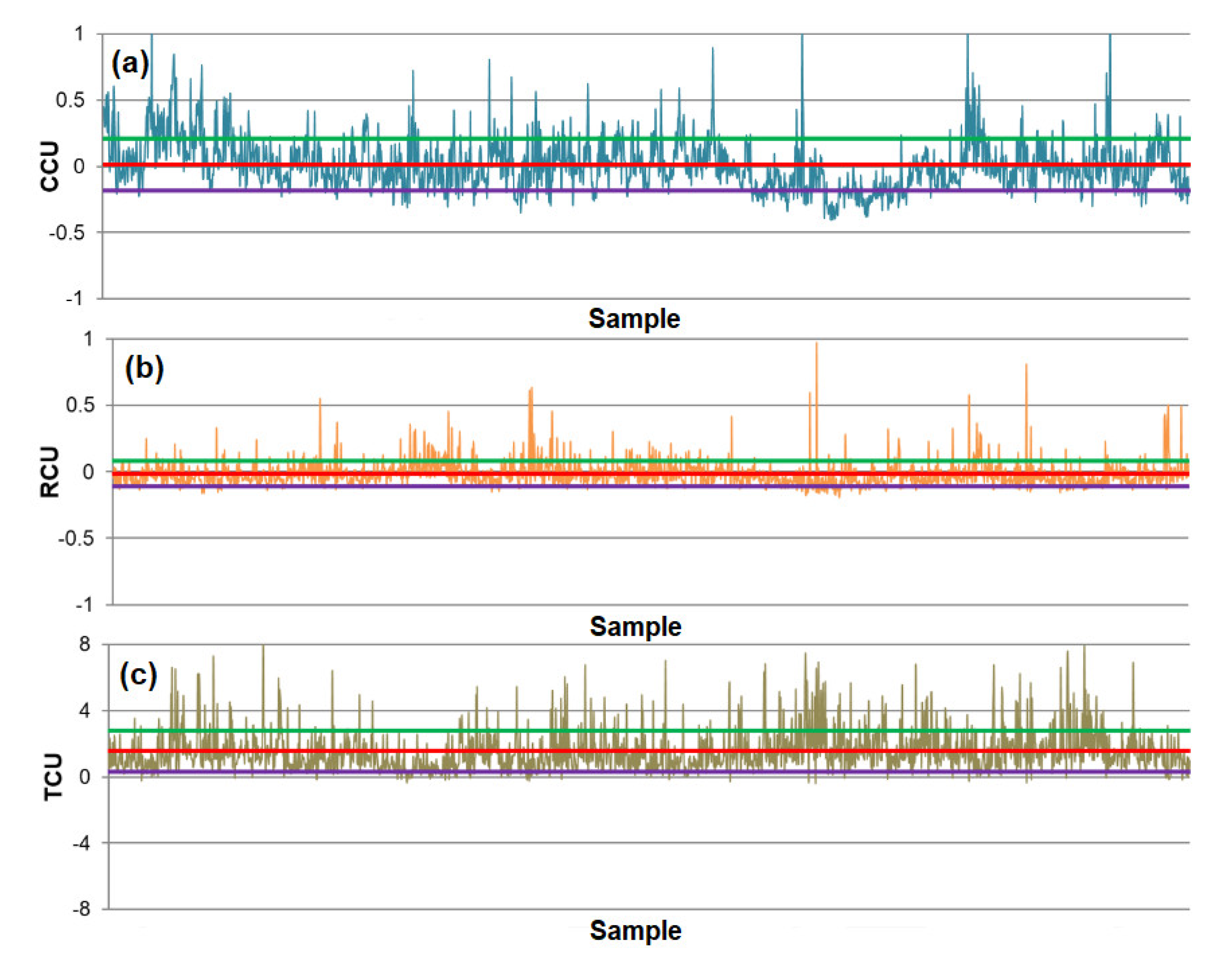
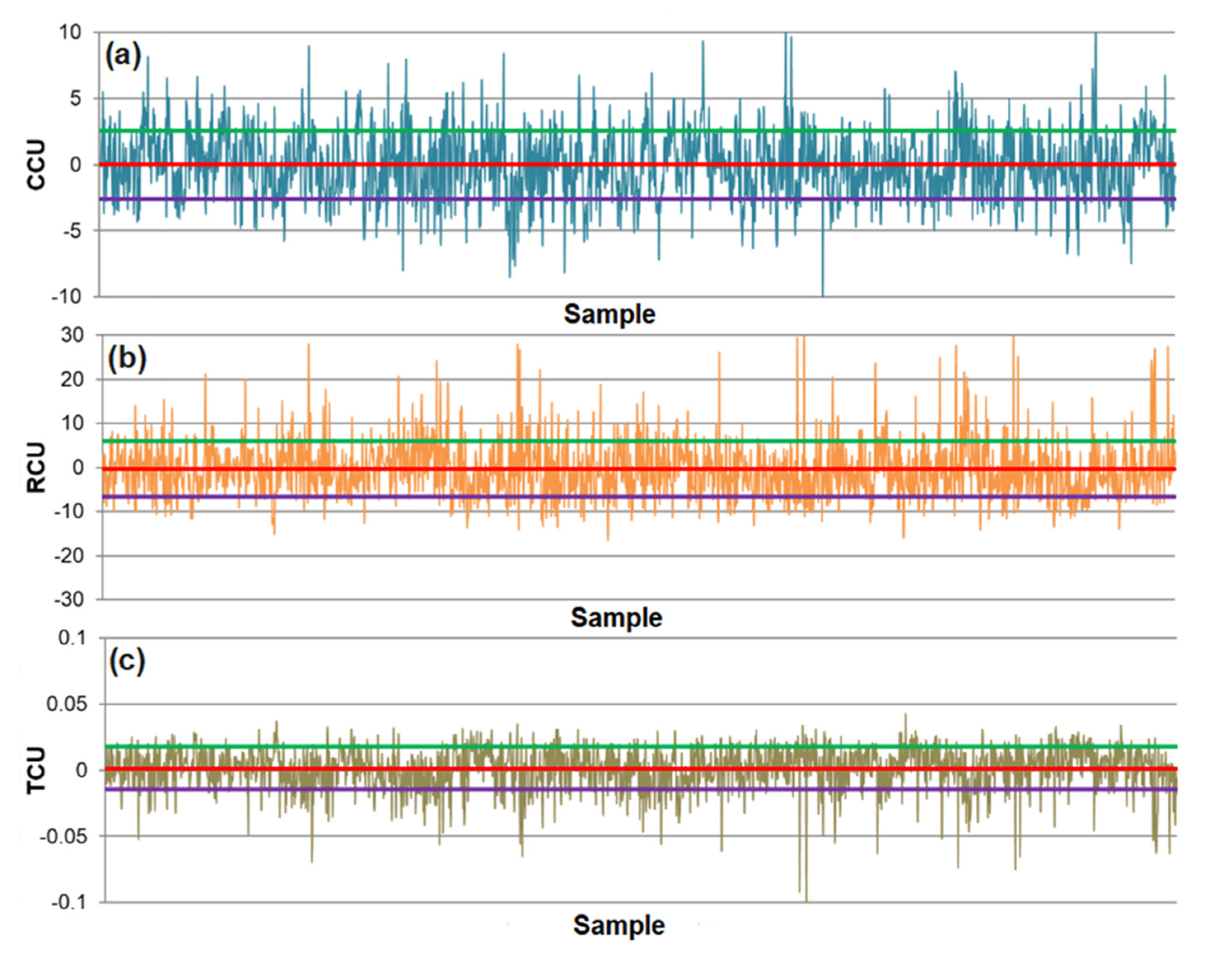
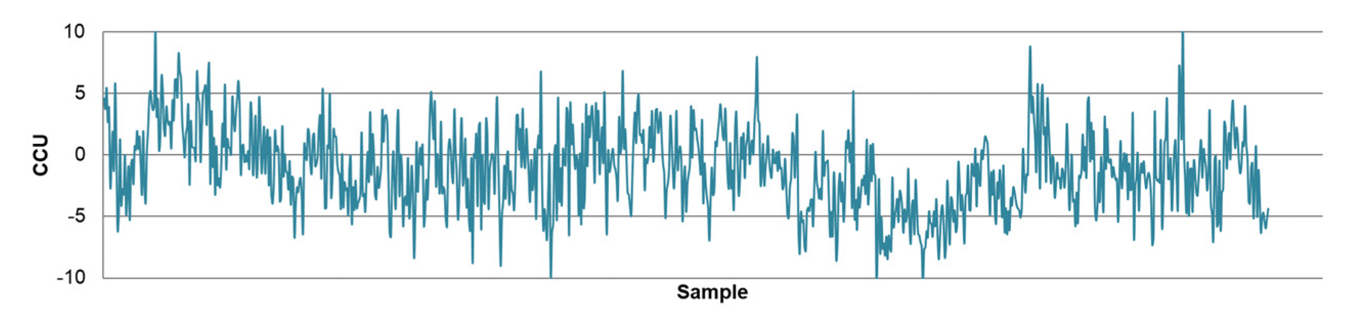
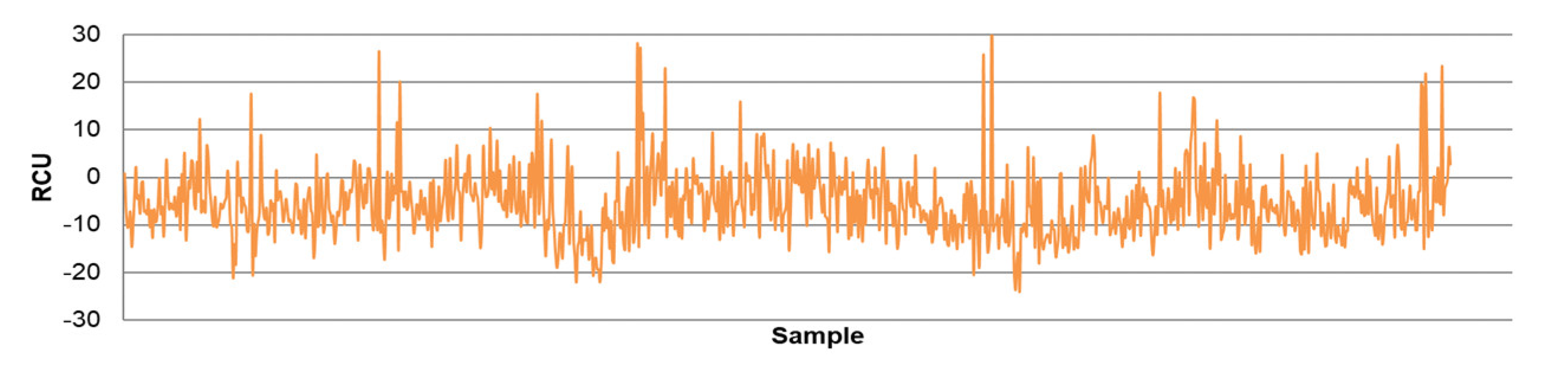
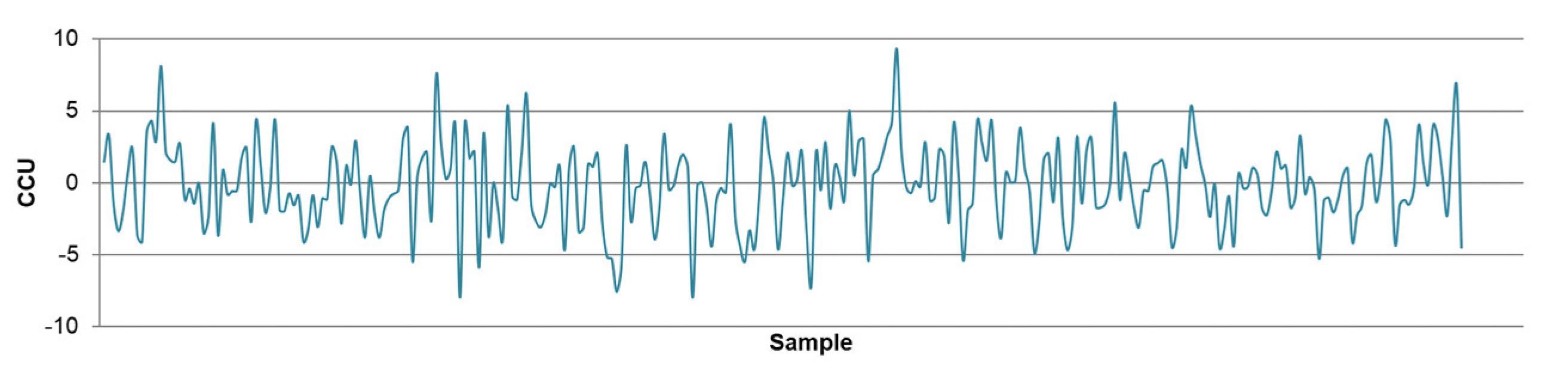
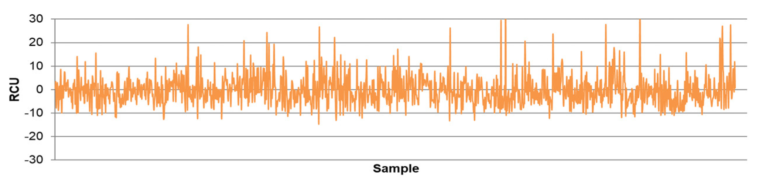
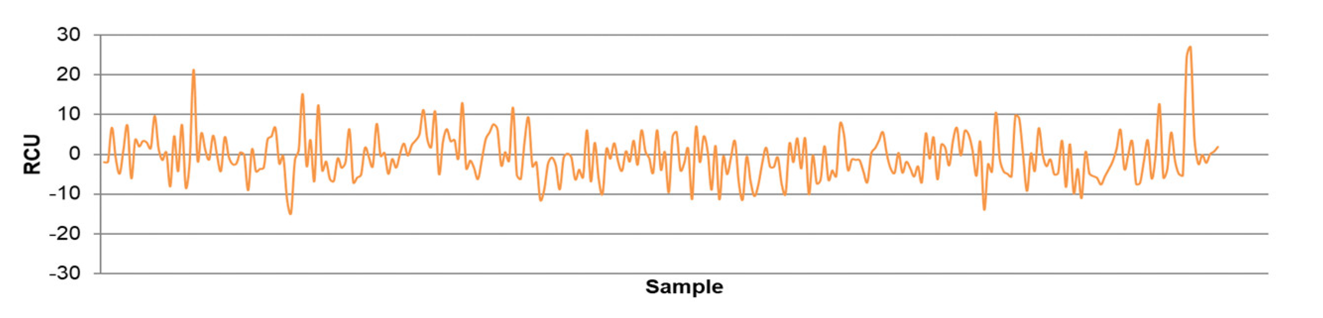
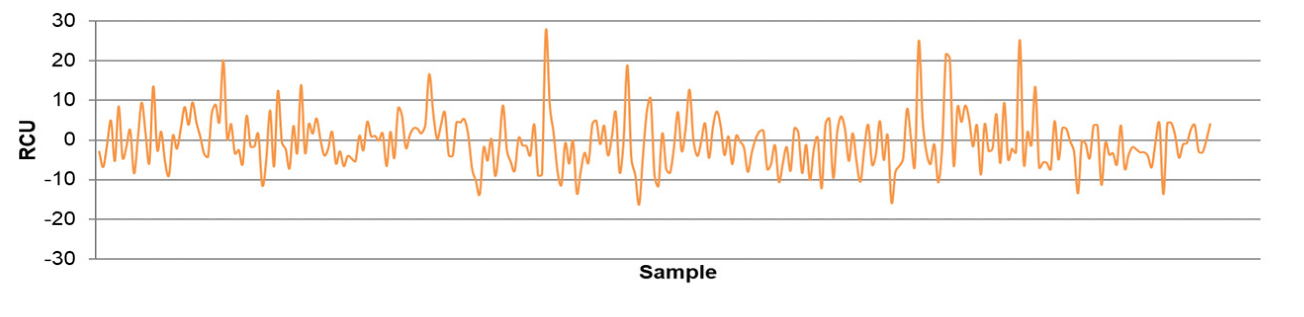
- The differences between predicted and actual values are relatively small for all models. The significant deviations between actual and predicted values most likely occurred due to the fluctuations in real process data that can be caused by various factors, such as changing process dynamics due to the downtime of the plant, oscillations in the process parameters that were considered constant during modeling, changes in the reagents’ quality, changes in process water quality, human factor, etc.
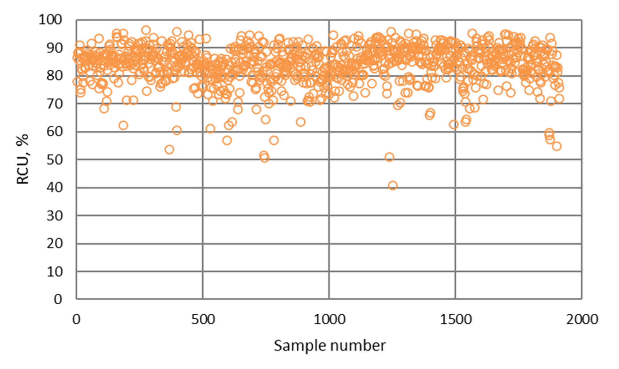
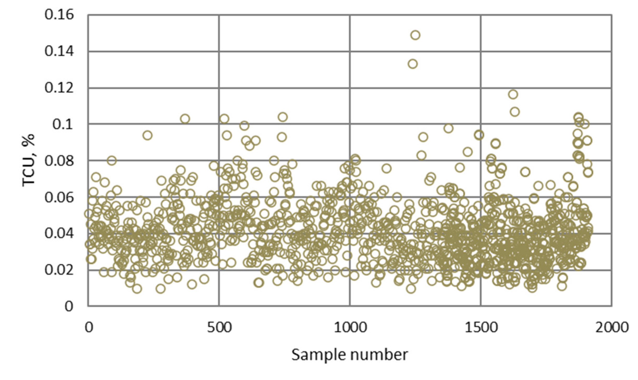
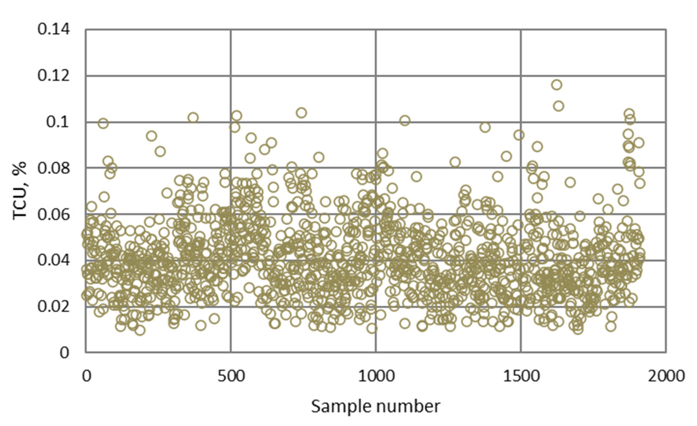
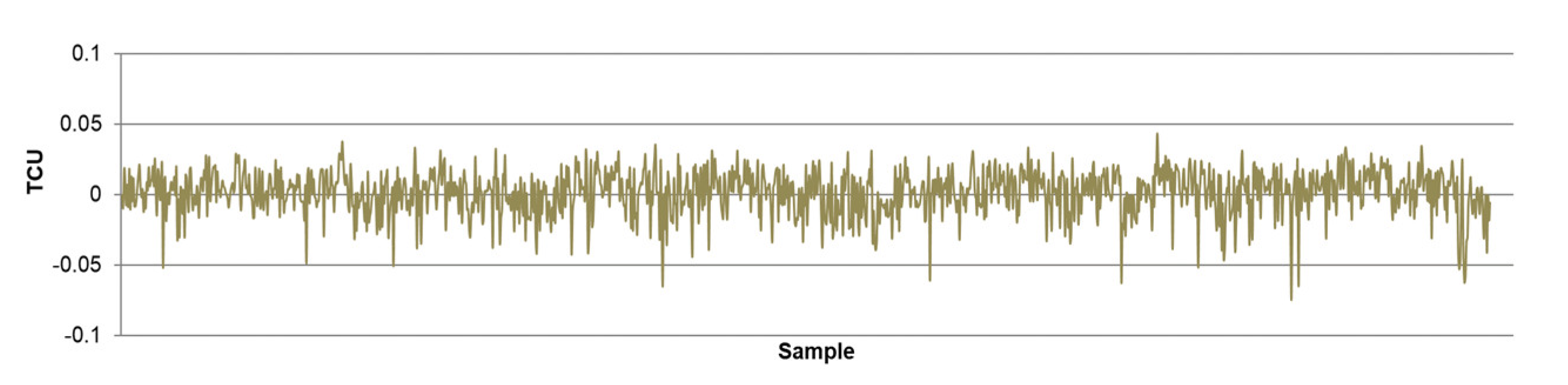
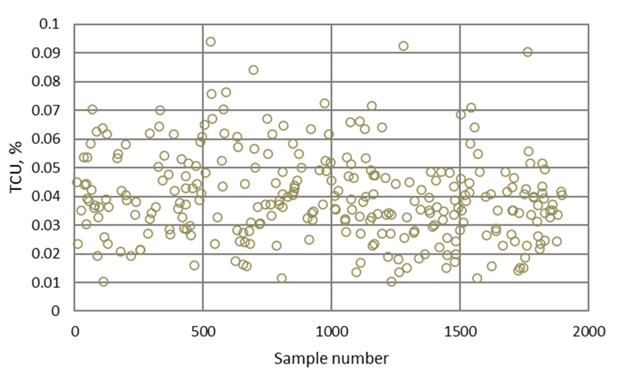
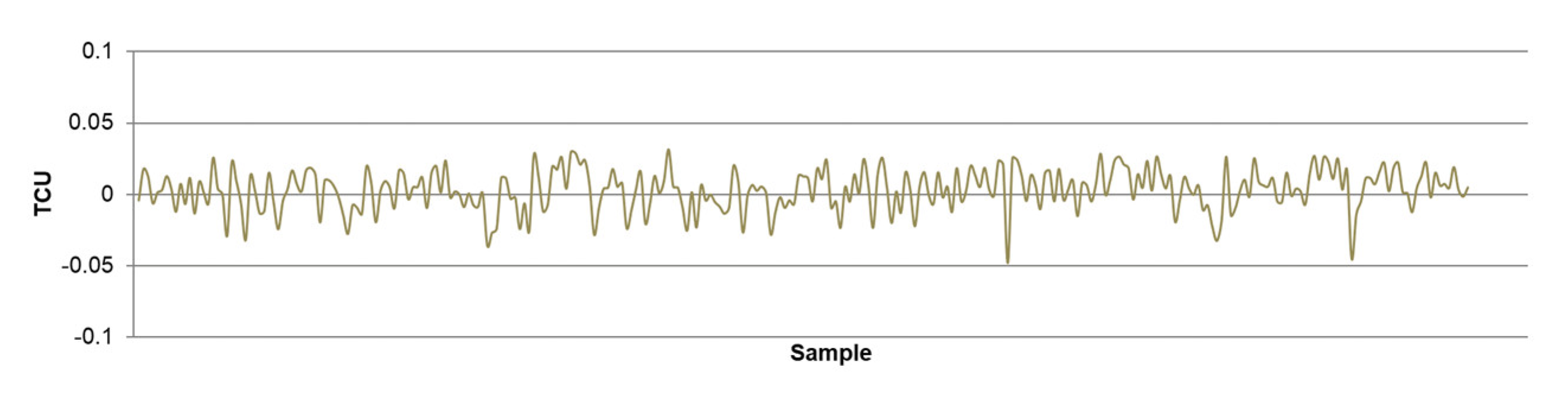
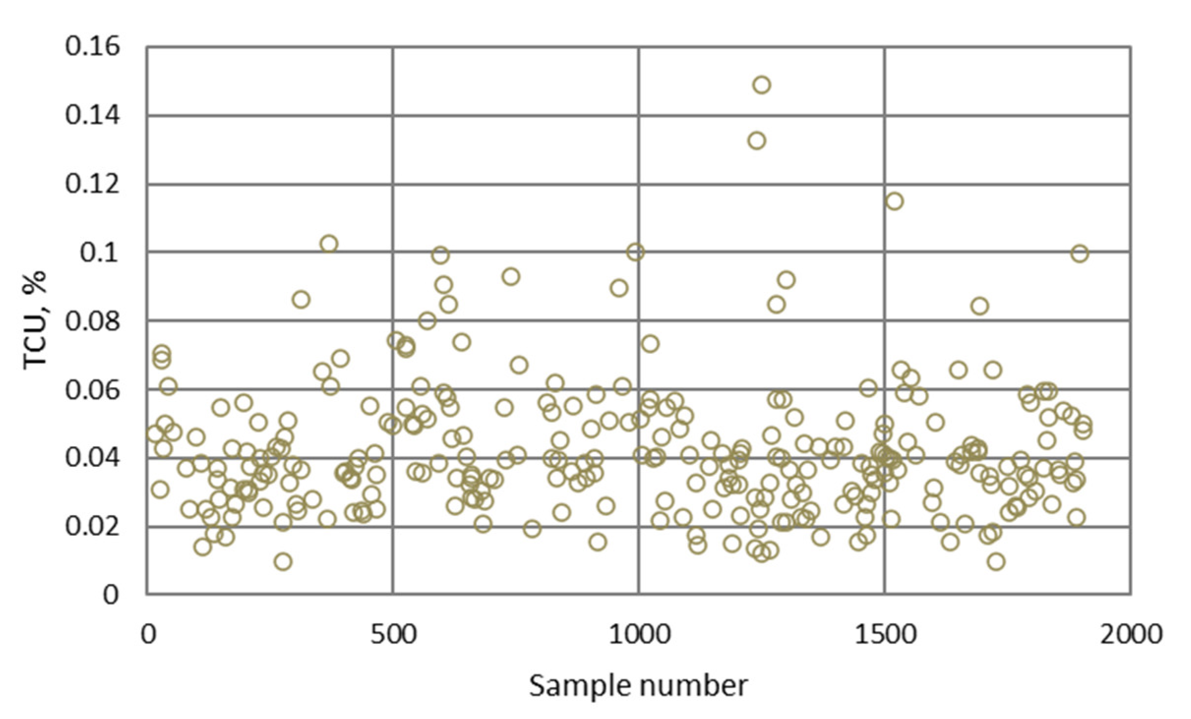
- The highest determination coefficients between actual and predicted values were obtained when modeling the copper recovery in the final concentrate, and the lowest when modeling the copper content in the final tailings. This can be applied to all models. The reason may lie in that the values of copper content in tailings vary in a relatively narrow range in relation to quality and recovery. Therefore, it may happen that the influences of completely different values of input parameters are integrated through very similar or the same copper contents in tailings, without this being taken into account during modeling. Such a situation could significantly affect the determination coefficient. Moreover, possible imperfections during tailings’ sampling (which are particularly linked to instabilities in the operation of the plant) should not be ignored, because the copper content in the samples is extremely low, and therefore proper sampling is of crucial importance for obtaining the precise chemical composition of the tailings.
- In accordance with the previous statement, the smallest standard deviations of the relative prediction error were obtained with the models that predict Cu recovery in the concentrate, and the largest with the models that predict Cu content in the tailings.
- By comparing the results of Mamdani and Takagi Sugeno fuzzy inference systems, it can be inferred that they demonstrate very similar predictive performance.
- Further research will be focused on the inclusion of other independent variables into the models, as well as on the modeling of individual parts of the flotation process depending on the availability (i.e., continual measurement) of process data to evaluate whether prediction results are improved or not.
- Sensitivity analysis of models, especially regarding the parameters considered constant, can be very helpful when it comes to improving the performances of the models and also represents the topic of future research.
- The application of more advanced software tools, as well as other soft computing methods, can also be effective in modeling such systems based on relatively large sets of input and output data.
Author Contributions
Funding
Acknowledgments
Conflicts of Interest
Appendix A
- Particle size analysis of grinding products;
- Pulp density;
- Pulp level;
- Pulp pH value;
- Reagents’ consumption.
Appendix B
Appendix B.1. Input Datasets


Appendix B.2. Output Datasets, Training, Testing and Validation Datasets


Appendix B.2.1. Fuzzy Logic Model Based on Mamdani Inference System—PMM
- Data from every even shift (955 in total) are determined for training,
- Data from every odd shift (955 in total) are determined for testing.
Training Datasets


| Statistical Parameters | Technological Indicator of the Flotation Process | ||
|---|---|---|---|
| CCU | RCU | TCU | |
| R2 | 0.971 | 0.992 | 0.851 |
| RMSE | 3.096 | 6.681 | 0.034 |
Testing Datasets


| Statistical Parameters | Technological Indicator of the Flotation Process | ||
|---|---|---|---|
| CCU | RCU | TCU | |
| R2 | 0.972 | 0.993 | 0.840 |
| RMSE | 3.049 | 6.613 | 0.035 |
Appendix B.2.2. Artificial Neural Network-Based Model for CCU Prediction—NN1
- A total of 60% of the data (1336 in total) are determined for training;
- A total of 15% of the data (287 in total) are determined for testing;
- A total of 15% of the data (287 in total) are determined for validation.


| Statistical Parameters | CCU | ||
|---|---|---|---|
| Training | Testing | Validation | |
| R2 | 0.983 | 0.981 | 0.978 |
| RMSE | 2.489 | 2.635 | 2.854 |
Appendix B.2.3. Artificial Neural Network-Based Model for RCU Prediction—NN2
- A total of 60% of the data (1336 in total) are determined for training;
- A total of 15% of the data (287 in total) are determined for testing;
- A total of 15% of the data (287 in total) are determined for validation.


| Statistical Parameters | RCU | ||
|---|---|---|---|
| Training | Testing | Validation | |
| R2 | 0.994 | 0.995 | 0.993 |
| RMSE | 6.291 | 5.762 | 6.767 |
Appendix B.2.4. Artificial Neural Network-Based Model for TCU Prediction—NN3
- A total of 60% of the data (1336 in total) are determined for training;
- A total of 15% of the data (287 in total) are determined for testing;
- A total of 15% of the data (287 in total) are determined for validation.


| Statistical Parameters | RCU | ||
|---|---|---|---|
| Training | Testing | Validation | |
| R2 | 0.873 | 0.884 | 0.829 |
| RMSE | 0.015 | 0.014 | 0.017 |
References
- Jovanović, I.; Magdalinović, N.; Kržanović, D.; Rajković, R. Comparative analysis of AI models in the modeling of flotation process. In Mining and Metallurgy Engineering Bor 3-4/2018; Mining and Metallurgy Engineering Bor: Bor, Serbia, 2018; pp. 27–32. ISSN 2334-8836. [Google Scholar]
- Nakhaei, F.; Sam, A.; Mosavi, M.R.; Zeidabadi, S. Prediction of copper grade at flotation column concentrate using artificial neural network. In Proceedings of the IEEE 10th International Conference on Signal Processing Proceedings, Beijing, China, 24–28 October 2010; pp. 1421–1424. [Google Scholar]
- Quintanilla, P.; Neethling, S.J.; Brito-Parada, P.R. Modelling for froth flotation control: A review. Miner. Eng. 2021, 162, 106718. [Google Scholar] [CrossRef]
- Jovanović, I. Model Inteligentnog Sistema Adaptivnog Upravljanja Procesom Prerade Rude. Ph.D. Thesis, Rudarsko-geološki Fakultet, Belgrade, Serbia, 2016; p. 217. (In Serbian). [Google Scholar]
- Jovanović, I.; Miljanović, I.; Jovanović, T. Soft computing-based modeling of flotation processes—A review. Miner. Eng. 2015, 84, 34–63. [Google Scholar] [CrossRef]
- Cisternas, L.A.; Lucay, F.A.; Botero, Y.L. Trends in Modeling, Design, and Optimization of Multiphase Systems in Minerals Processing. Minerals 2020, 10, 22. [Google Scholar] [CrossRef] [Green Version]
- Dos Santos, N.A.; Savassi, O.; Peres, A.E.C.; Martins, A.H. Modelling flotation with a flexible approach—Integrating different models to the compartment model. Miner. Eng. 2014, 66–68, 68–76. [Google Scholar] [CrossRef]
- Seppälä, P.; Sorsa, A.; Paavola, M.; Ruuska, J.; Remes, A.; Kumar, H.; Lamberg, P.; Leiviskä, K. Development and calibration of a dynamic flotation circuit model. Miner. Eng. 2016, 96–97, 168–176. [Google Scholar] [CrossRef]
- Suazo, C.J.; Kracht, W.; Alruiz, O.M. Geometallurgical modelling of the Collahuasi flotation circuit. Miner. Eng. 2010, 23, 137–142. [Google Scholar] [CrossRef]
- Al-Thyabat, S. On the optimization of froth flotation by the use of artificial neural network. J. China Univ. Min. Technol. 2008, 18, 418–426. [Google Scholar] [CrossRef]
- Farghaly, M.; Serwa, A.; Ahmed, M. Optimizing the Egyptian Coal Flotation Using an Artificial Neural Network. J. Min. World Express 2012, 1, 27–33. [Google Scholar]
- Jorjani, E.; Mesroghli, S.; Chelgani, S.C. Prediction of operational parameters effect on coal flotation using artificial neural network. J. Univ. Sci. Technol. Beijing 2008, 15, 528–533. [Google Scholar] [CrossRef]
- Nakhaei, F.; Mosavi, M.R.; Sam, A.; Vaghei, Y. Recovery and grade accurate prediction of pilot plant flotation column concentrate: Neural network and statistical techniques. Int. J. Miner. Process. 2012, 110–111, 140–154. [Google Scholar] [CrossRef]
- Nakhaei, F.; Irannajad, M. Comparison between neural networks and multiple regression methods in metallurgical performance modeling of flotation column. Physicochem. Probl. Miner. Process. 2013, 49, 255–266. [Google Scholar]
- Nakhaei, F.; Irannajad, M. Forecasting grade and recovery of flotation column concentrate using radial basis function and layer recurrent neural networks. AWERProcedia Inf. Technol. Comput. Sci. 2013, 4, 454–473. [Google Scholar]
- Jahedsaravani, A.; Marhaban, M.H.; Massinaei, M. Application of statistical and intelligent techniques for modeling of metallurgical performance of a batch flotation process. Chem. Eng. Commun. 2016, 203, 151–160. [Google Scholar] [CrossRef]
- Massinaei, M.; Sedaghati, M.R.; Rezvani, R.; Mohammadzadeh, A.A. Using data mining to assess and model the metallurgical efficiency of a copper concentrator. Chem. Eng. Commun. 2014, 201, 1314–1326. [Google Scholar] [CrossRef]
- Zhang, Y.; Chen, H.; Yang, B.; Fu, S.; Yu, J.; Wang, Z. Prediction of phosphate concentrate grade based on artificial neural network modeling. Results Phys. 2018, 11, 625–628. [Google Scholar] [CrossRef]
- Abdulhussein, S.A.; Alwared, A.I. The use of Artificial Neural Network (ANN) for modeling of Cu (II) ion removal from aqueous solution by flotation and sorptive flotation process. Environ. Technol. Innov. 2019, 13, 353–363. [Google Scholar] [CrossRef]
- Gholami, A.; Movahedifar, M.; Khoshdast, H.; Hassanzadeh, A. Hybrid Serving of DOE and RNN-Based Methods to Optimize and Simulate a Copper Flotation Circuit. Minerals 2022, 12, 857. [Google Scholar] [CrossRef]
- Aldrich, C.; Marais, C.; Shean, B.J.; Cilliers, J.J. Online monitoring and control of froth flotation systems with machine vision: A review. Int. J. Miner. Process. 2010, 96, 1–13. [Google Scholar] [CrossRef]
- Marais, C.; Aldrich, C. The estimation of platinum flotation grade from froth image features by using artificial neural networks. J. South. Afr. Inst. Min. Metall. 2011, 111, 81–85. [Google Scholar]
- Marais, C.; Aldrich, C. Estimation of platinum flotation grades from froth image data. Miner. Eng. 2011, 24, 433–441. [Google Scholar] [CrossRef]
- Jahedsaravani, A.; Marhaban, M.H.; Massinaei, M. Prediction of the metallurgical performances of a batch flotation system by image analysis and neural networks. Miner. Eng. 2014, 69, 137–145. [Google Scholar] [CrossRef]
- Hosseini, M.R.; Haji Amin Shirazi, H.; Massinaei, M.; Mehrshad, N. Modeling the Relationship between Froth Bubble Size and Flotation Performance Using Image Analysis and Neural Networks. Chem. Eng. Commun. 2015, 202, 911–919. [Google Scholar] [CrossRef]
- Wang, J.-S.; Han, S.; Shen, N.-N.; Li, S.-X. Features Extraction of Flotation Froth Images and BP Neural Network Soft-Sensor Model of Concentrate Grade Optimized by Shuffled Cuckoo Searching Algorithm. Sci. World J. 2014, 2014, 208094. [Google Scholar] [CrossRef] [Green Version]
- Haiyang, Z.; Yali, K.; Guanghui, W.; Li, J. Soft Sensor Model for Coal Slurry Ash Content Based on Image grey characteristics. Int. J. Coal Prep. Util. 2014, 34, 24–37. [Google Scholar] [CrossRef]
- Nakhaei, F.; Irannajad, M.; Mohammadnejad, S. Column flotation performance prediction: PCA, ANN and image analysis-based approaches. Physicochem. Probl. Miner. Process. 2019, 55, 1298–1310. [Google Scholar]
- Nakhaei, F.; Irannajad, M.; Mohammadnejad, S. A comprehensive review of froth surface monitoring as an aid for grade and recovery prediction of flotation process. Part A: Structural features. Energy Sources Part A Recovery Util. Environ. Eff. 2019. [Google Scholar] [CrossRef]
- Zhang, H.; Tang, Z.; Xie, Y.; Gao, X.; Chen, Q.; Gui, W. Long short-term memory-based grade monitoring in froth flotation using a froth video sequence. Miner. Eng. 2021, 160, 106677. [Google Scholar] [CrossRef]
- Fu, Y.; Aldrich, C. Flotation froth image recognition with convolutional neural networks. Miner. Eng. 2019, 132, 183–190. [Google Scholar] [CrossRef]
- Pu, Y.; Szmigiel, A.; Chen, J.; Apel, D.B. FlotationNet: A hierarchical deep learning network for froth flotation recovery prediction. Powder Technol. 2020, 375, 317–326. [Google Scholar] [CrossRef]
- Zarie, M.; Jahedsaravani, A.; Massinaei, M. Flotation froth image classification using convolutional neural networks. Miner. Eng. 2020, 155, 106443. [Google Scholar] [CrossRef]
- Wen, Z.; Zhou, C.; Pan, J.; Nie, T.; Zhou, C.; Lu, Z. Deep learning-based ash content prediction of coal flotation concentrate using convolutional neural network. Miner. Eng. 2021, 174, 107251. [Google Scholar] [CrossRef]
- Gao, X.; Tang, Z.; Xie, Y.; Zhang, H.; Gui, W. A layered working condition perception integrating handcrafted with deep features for froth flotation. Miner. Eng. 2021, 170, 107059. [Google Scholar] [CrossRef]
- Jahan, A.; Edwards, K.L.; Bahraminasab, M. Multi-Attribute Decision-Making for Ranking of Candidate Materials. In Multi-criteria Decision Analysis for Supporting the Selection of Engineering Materials in Product Design, 2nd ed.; Jahan, A., Edwards, K.L., Bahraminasab, M., Eds.; Butterworth-Heinemann: Oxford, UK, 2016; pp. 81–126. [Google Scholar]
- Naderloo, L.; Alimardani, R.; Omid, M.; Sarmadian, F.; Javadikia, P.; Torabi, M.Y.; Alimardani, F. Application of ANFIS to predict crop yield based on different energy inputs. Measurement 2012, 45, 1406–1413. [Google Scholar] [CrossRef]
- Amiryousefi, M.R.; Mohebbi, M.; Khodaiyan, F.; Asadi, S. An empowered adaptive neuro-fuzzy inference system using self-organizing map clustering to predict mass transfer kinetics in deep-fat frying of ostrich meat plates. Comput. Electron. Agric. 2011, 76, 89–95. [Google Scholar] [CrossRef]
- Sitorus, F.; Brito-Parada, P.R. Equipment selection in mineral processing—A sensitivity analysis approachfor a fuzzy multiple criteria decision making model. Miner. Eng. 2020, 150, 106261. [Google Scholar] [CrossRef]
- Zhang, W.; Liu, D.; Du, Y.; Liu, R.; Wang, D.; Yu, L.; Wen, S. Mill Feed Control System and Algorithm Based on Python. Minerals 2022, 12, 804. [Google Scholar] [CrossRef]
- Jovanović, I.; Nešković, J.; Petrović, S.; Milanović, D. A hybrid approach to modeling the flotation process from the “Veliki Krivelj” plant. In Mining and Metallurgy Engineering Bor 1-2/2018; Mining and Metallurgy Engineering Bor: Bor, Serbia, 2018; pp. 1–10. ISSN 2334-8836. [Google Scholar]
- Lott, G.D.; Da Silva, M.T.; Cota, L.P.; Guimarães, F.G.; Euzébio, T.A.M. Fuzzy Decision Support System for the Calibration of Laboratory-Scale Mill Press Parameters. IEEE Access 2021, 9, 24901–24912. [Google Scholar] [CrossRef]
- Carvalho, M.T.; Durão, F. Performance of a flotation column fuzzy controller. In Computers and Computational Engineering in Control; Mastorakis, N.E., Ed.; World Scientific and Engineering Society Press: Athens, Greece, 1999; pp. 220–225. [Google Scholar]
- Carvalho, M.T.; Durão, F. Control of a flotation column using fuzzy logic inference. Fuzzy Sets Syst. 2002, 125, 121–133. [Google Scholar] [CrossRef]
- Vieira, S.M.; Sousa, J.M.C.; Durão, F.O. Fuzzy modelling strategies applied to a column flotation process. Miner. Eng. 2005, 18, 725–729. [Google Scholar] [CrossRef]
- Liao, Y.; Liu, J.; Wang, Y.; Cao, Y. Simulating a fuzzy level controller for flotation columns. Min. Sci. Technol. 2011, 21, 815–818. [Google Scholar] [CrossRef]
- Jahedsaravani, A.; Mehrshad, N.; Massinaei, M. Fuzzy-based modeling and control of an industrial flotation column. Chem. Eng. Commun. 2014, 201, 896–908. [Google Scholar]
- Zhou, K.; Zhou, X. Adaptive fuzzy local ternary pattern for mineral flotation froth image edge detection. IFAC Pap. 2018, 51, 235–240. [Google Scholar] [CrossRef]
- Liang, Y.; He, D.; Su, X.; Wang, F. Fuzzy distributional robust optimization for flotation circuit configurations based on uncertainty theories. Miner. Eng. 2020, 156, 106433. [Google Scholar] [CrossRef]
- Ali, S. Mathematical Models for the Efficiency of Flotation Process for North Waziristan Copper. Ph.D. Thesis, University of Education, Lahore, Pakistan, 2007, 2007; p. 167. [Google Scholar]
- Yang, L.; Liu, T.; Ren, W.; Sun, W. Fuzzy Neural Network for Studying Coupling between Drilling Parameters. ACS Omega 2021, 6, 24351–24361. [Google Scholar] [CrossRef]
- Zadeh, L.A. A new direction in AI: Toward a computational theory of perceptions. AI Mag. 2001, 22, 73. [Google Scholar]
- Latha, B.; Senthilkumar, V. Analysis of thrust force in drilling glass fiber-reinforced plastic composites using fuzzy logic. Mater. Manuf. Process. 2009, 24, 509–516. [Google Scholar] [CrossRef]
- Şahin, M.; Erol, R. Prediction of Attendance Demand in European Football Games: Comparison of ANFIS, Fuzzy Logic, and ANN. Comput. Intell. Neurosci. 2018, 2018, 5714872. [Google Scholar] [CrossRef]
- Lerkkasemsan, N.; Achenie, L.E. Pyrolysis of biomass–fuzzy modeling. Renew. Energy 2014, 66, 747–758. [Google Scholar] [CrossRef]
- Bhowmik, S.; Panua, R.; Ghosh, S.K.; Paul, A.; Debroy, D. Prediction of performance and exhaust emissions of diesel engine fuelled with adulterated diesel: An artificial neural network assisted fuzzy-based topology optimization. Energy Environ. 2018, 29, 1413–1437. [Google Scholar] [CrossRef]
- Ghodrati, S.; Nakhaei, F.; VandGhorbany, O.; Hekmati, M. Modeling and optimization of chemical reagents to improve copper flotation performance using response surface methodology. Energy Sources Part A Recovery Util. Environ. Eff. 2020, 42, 1633–1648. [Google Scholar] [CrossRef]
- Asghari, M.; Nakhaei, F.; VandGhorbany, O. Copper recovery improvement in an industrial flotation circuit: A case study of Sarcheshmeh copper mine. Energy Sources Part A Recovery Util. Environ. Eff. 2019, 41, 761–778. [Google Scholar] [CrossRef]
- Ćalić, N. Teorijski Osnovi Pripreme Mineralnih Sirovina; Rudarsko-geološki fakultet Beograd—Faculty of Mining and Geology: Belgrade, Serbia, 1990; p. 496. (In Serbian) [Google Scholar]
- Jassbi, J.; Alavi, S.H.; Serra, P.J.A.; Ribeiro, R.A. Transformation of a Mamdani FIS to First Order Sugeno FIS. In Proceedings of the IEEE International Conference on Fuzzy Systems, London, UK, 23–26 July 2007; pp. 5–10. [Google Scholar]
- Nakhaei, F.; Sam, A.; Mosavi, M.R. Concentrate Grade Prediction in an Industrial Flotation Column using the Artificial Neural Network. Arab. J. Sci. Eng. 2013, 38, 1011–1023. [Google Scholar] [CrossRef]
- Nakhaei, F.; Irannajad, M. Application and comparison of RNN, RBFNN and MNLR approaches on prediction of flotation column performance. Int. J. Min. Sci. Technol. 2015, 25, 983–990. [Google Scholar] [CrossRef]
- Ying, X. An Overview of Overfitting and its Solutions. J. Phys. Conf. Ser. 2019, 1168, 022022. [Google Scholar] [CrossRef]
- Available online: https://towardsdatascience.com/the-secret-neural-network-formula-70b41f0da767 (accessed on 20 October 2020).
- Sarker, I.H. Deep Learning: A Comprehensive Overview on Techniques, Taxonomy, Applications and Research Directions. SN Comput. Sci. 2021, 2, 420. [Google Scholar] [CrossRef] [PubMed]
- Nikolić, I.; Jovanović, I.; Mihajlović, I.; Miljanović, I. Analiza proizvodnje koncentrata bakra sistemskim pristupom (Analysis of copper concentrate production by systemic approach). Bakar 2016, 40, 33–50. (In Serbian) [Google Scholar]


| Type of Variable | Label in the Model | Unit of Measurement |
|---|---|---|
| Copper content in the feed | FCU | % |
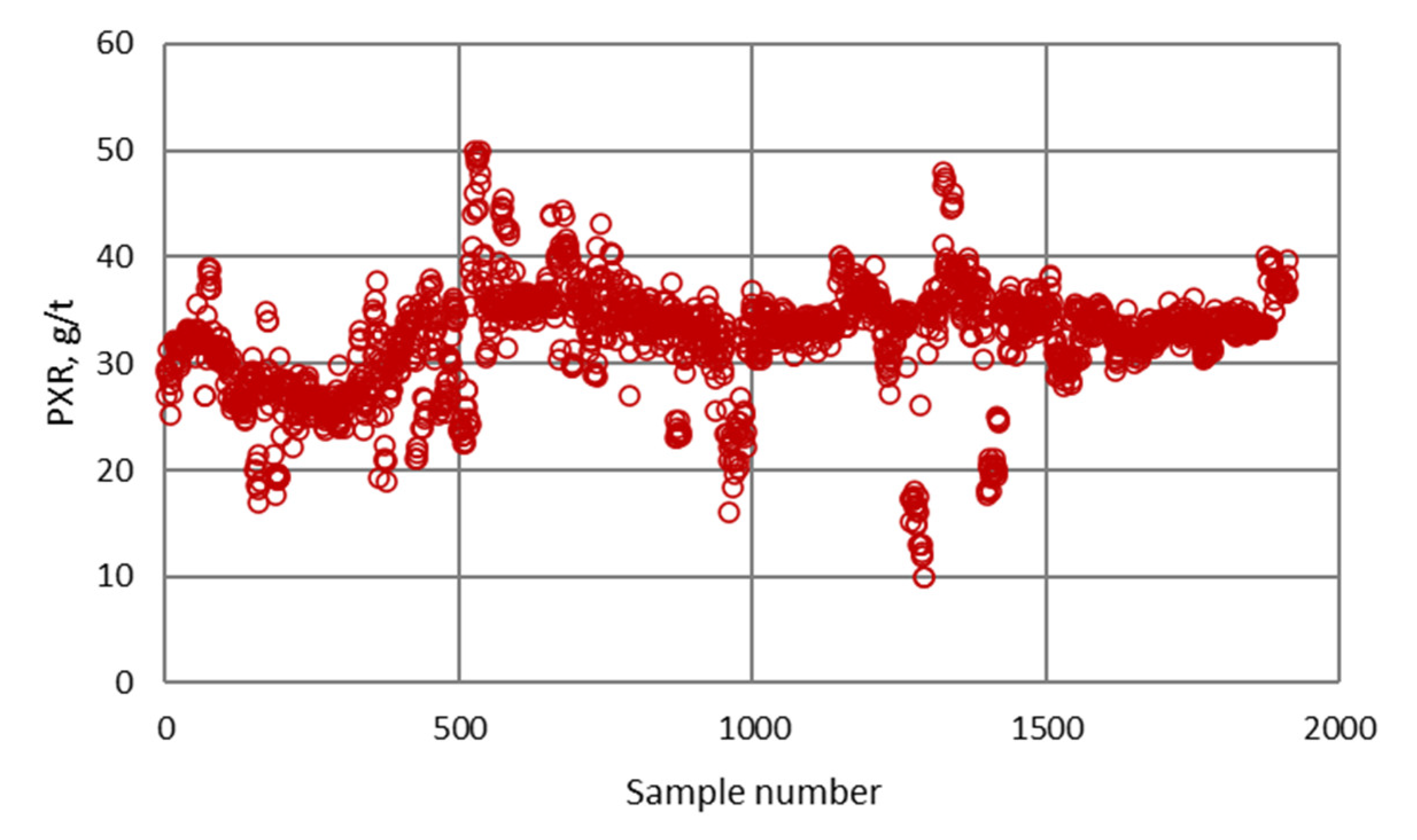
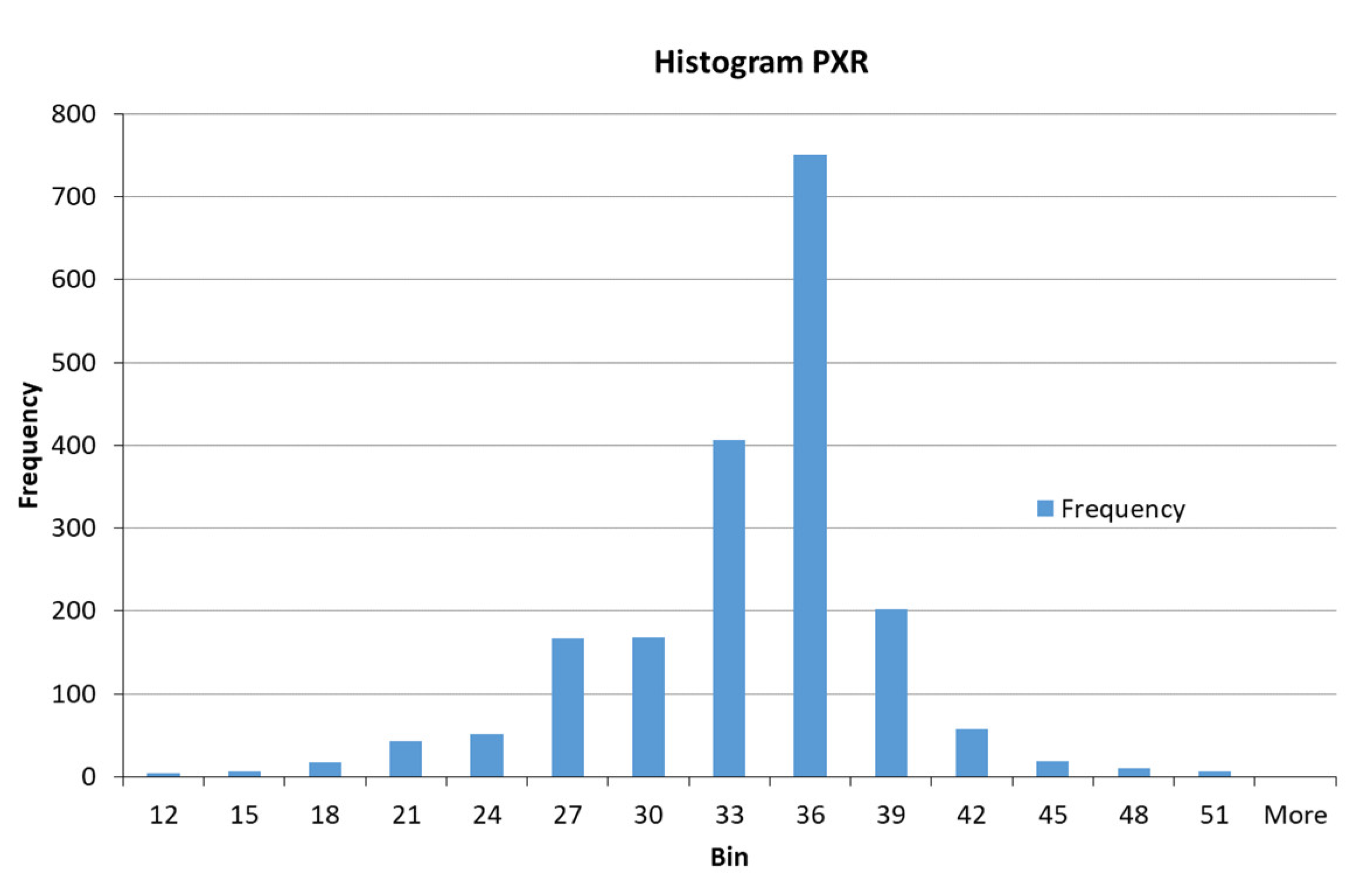
| Collector consumption at rougher flotation circuit | PXR | g/t |
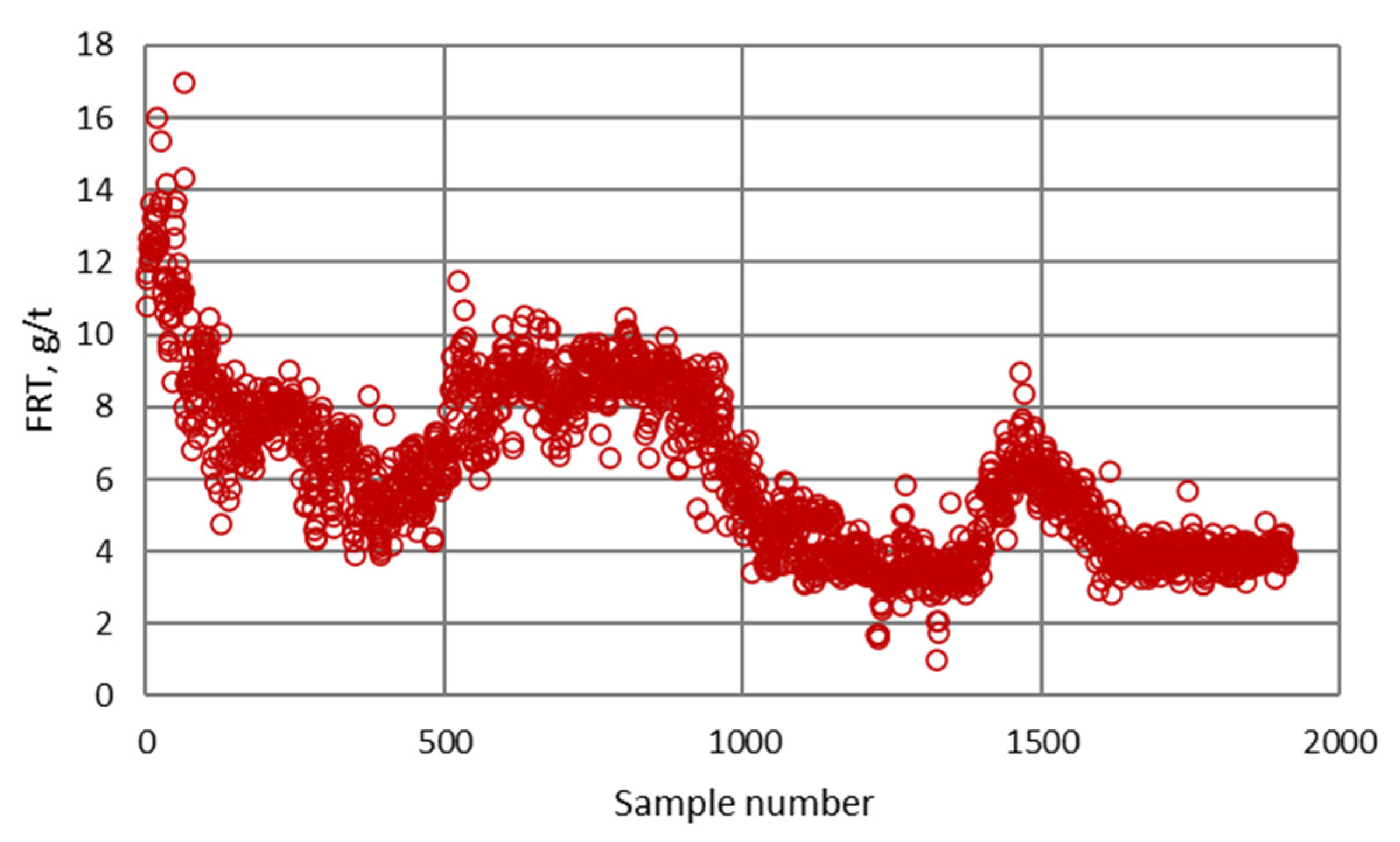
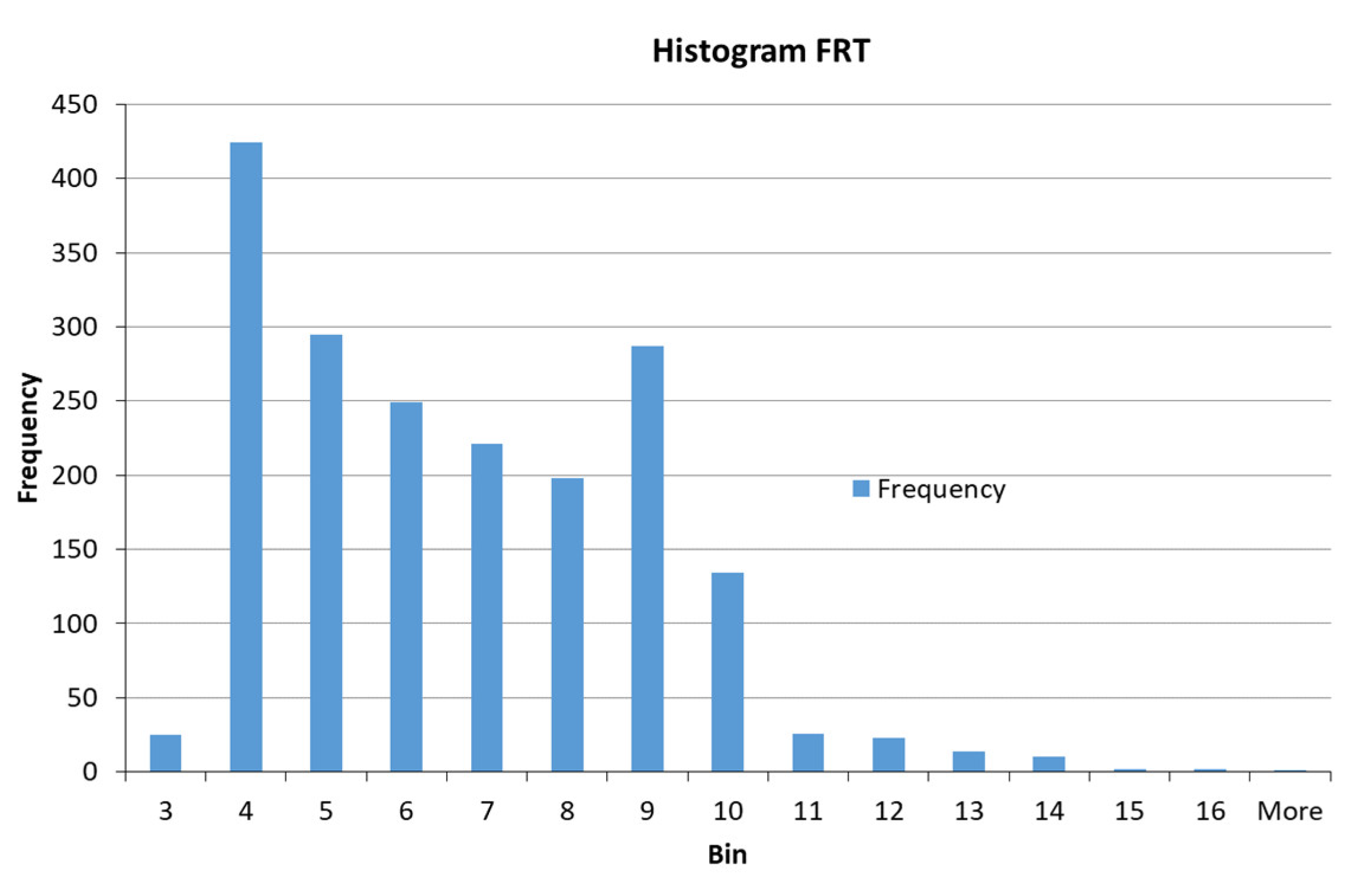
| Frother consumption | FRT | g/t |
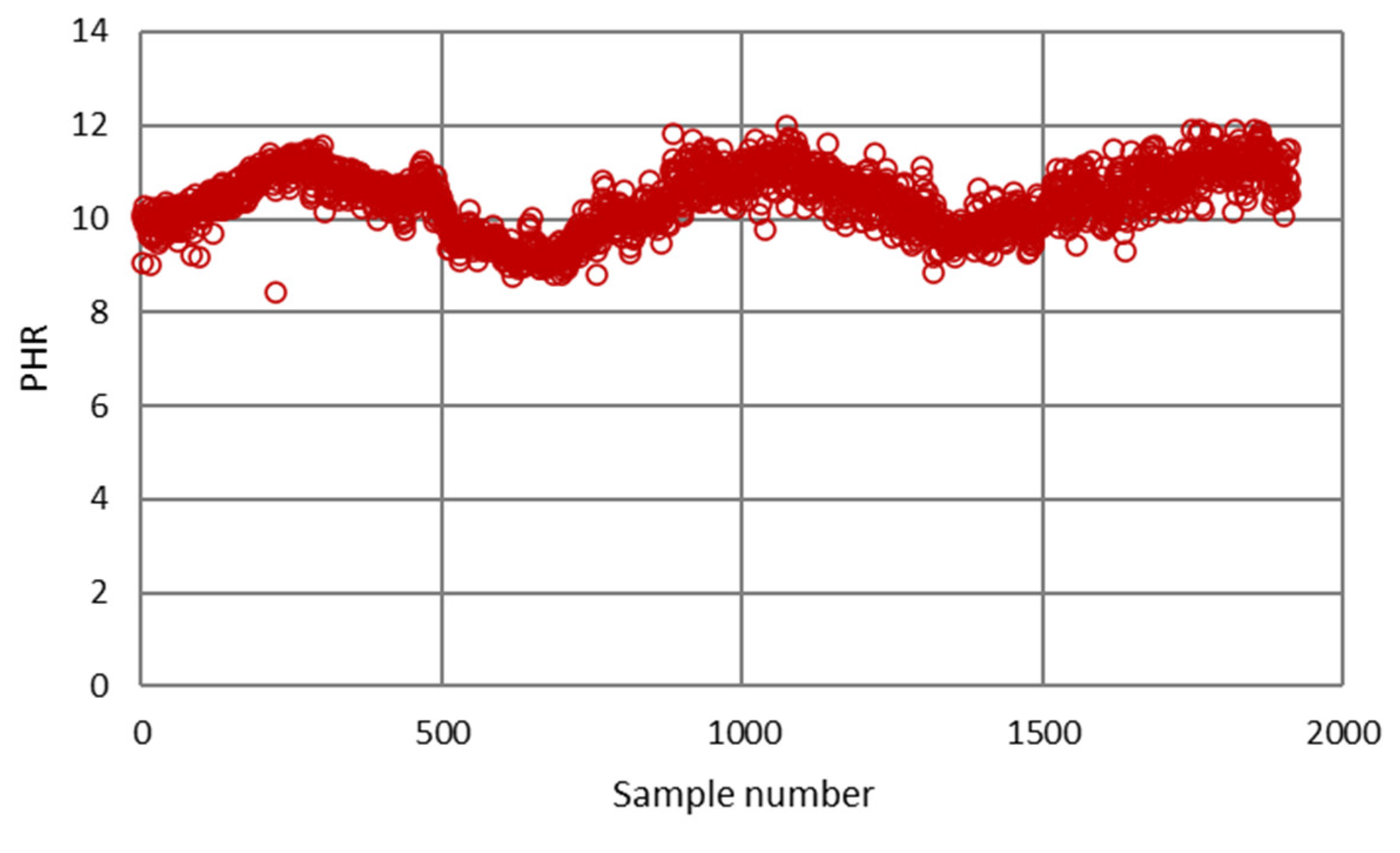
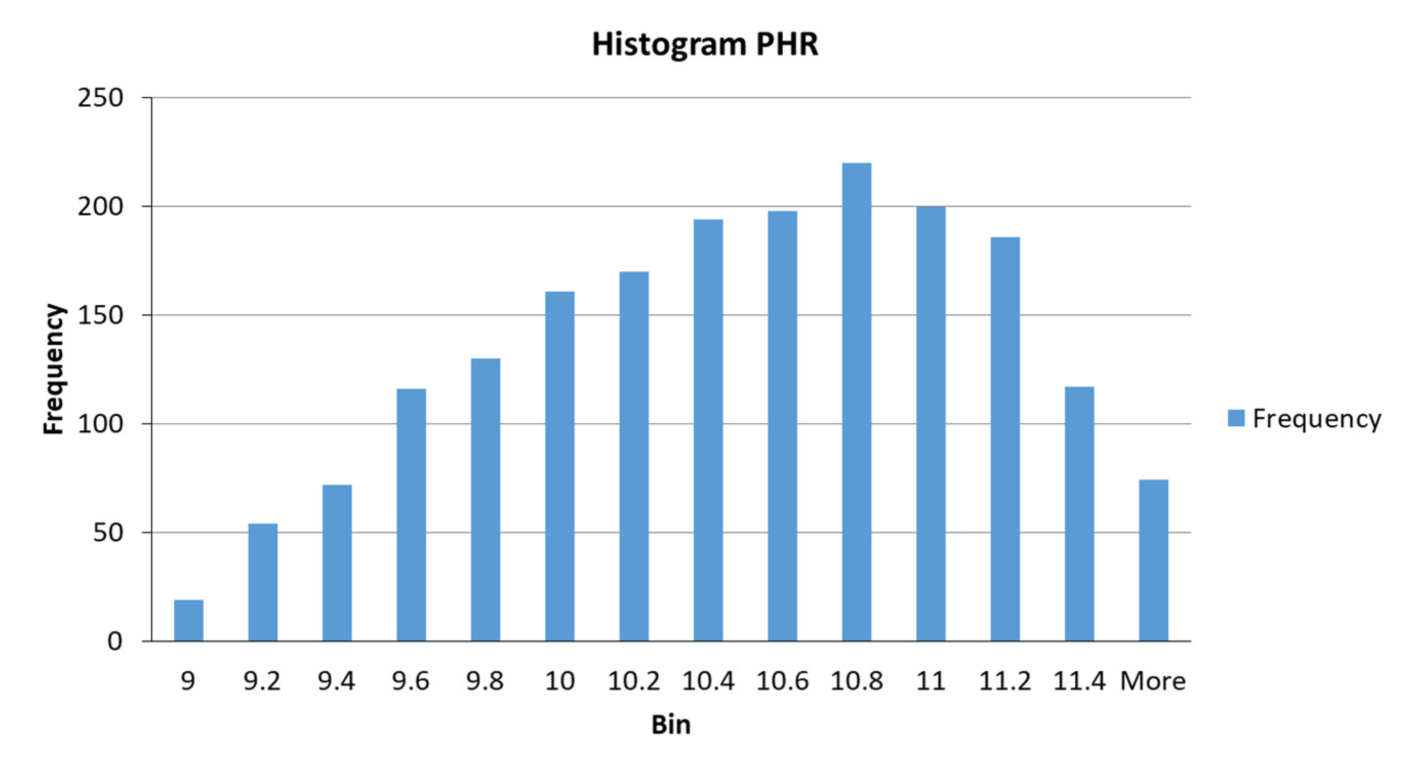
| pH value of slurry at rougher flotation circuit | PHR | - |
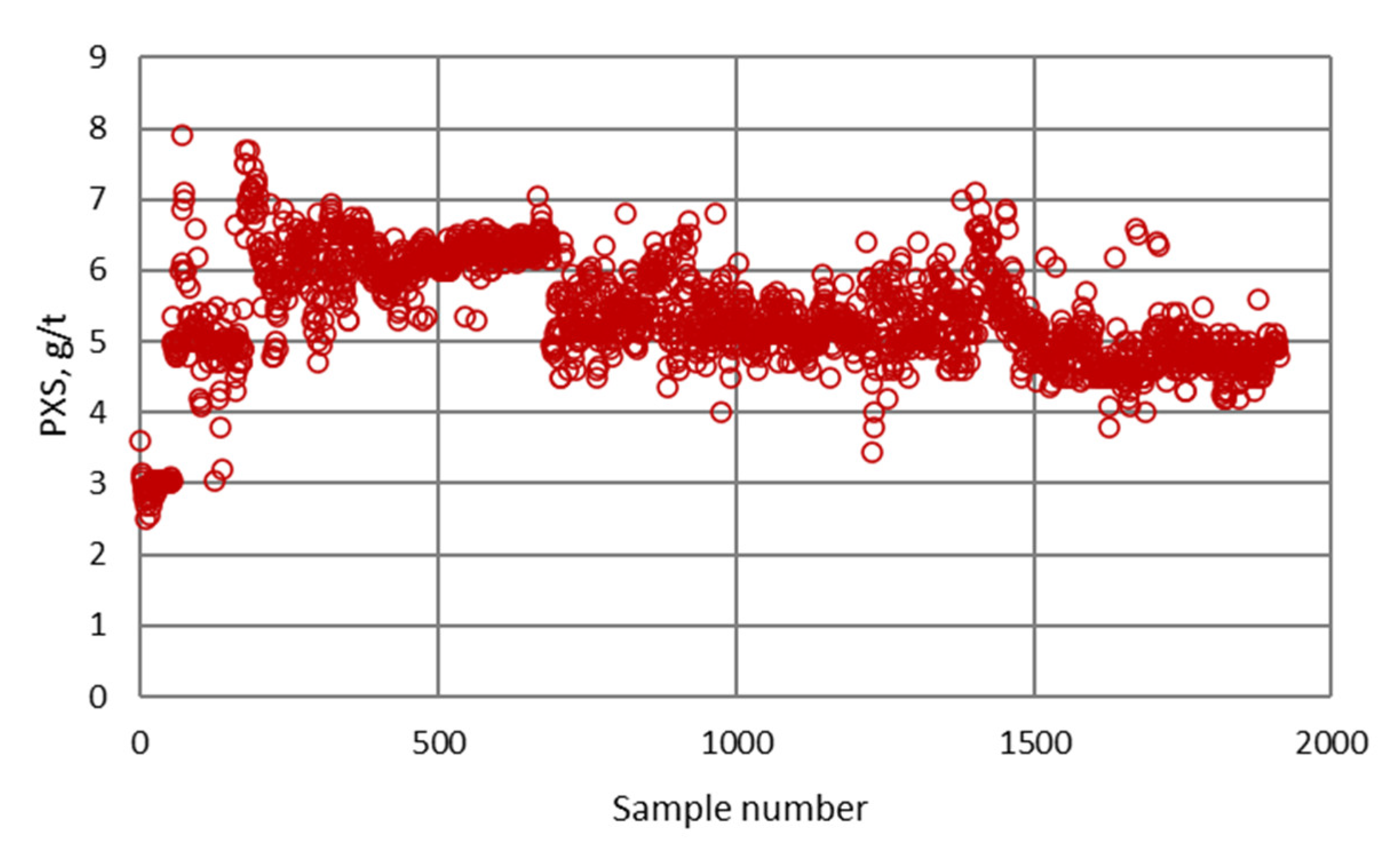
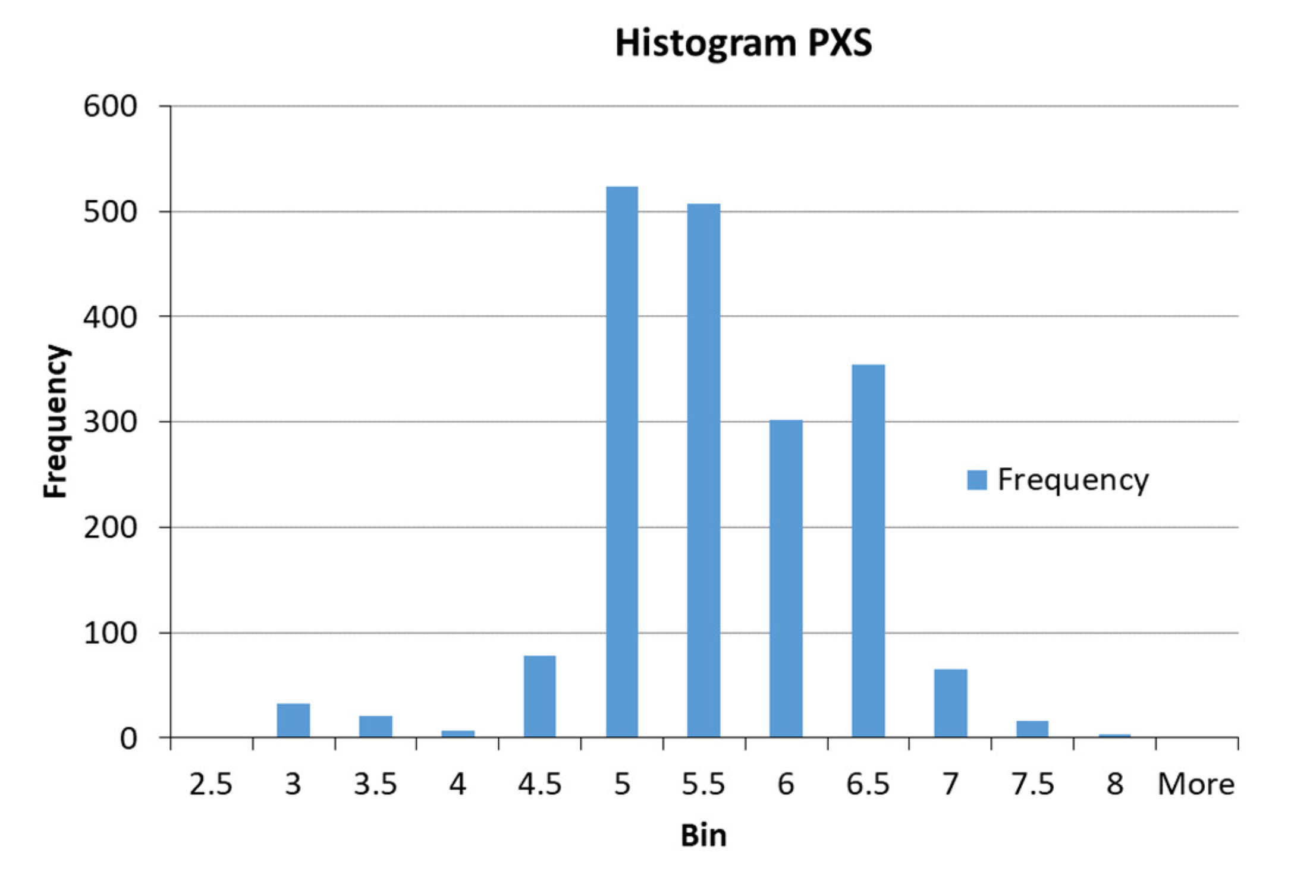
| Collector consumption at scavenger flotation circuit | PXS | g/t |
| Parameter | Value | Unit of Measurement |
|---|---|---|
| Grinding fineness | 58 | % of class −74 + 0 μm |
| Regrinding fineness | 85 | % of class −74 + 0 μm |
| Pulp density in rougher flotation circuit | 1190 | g/L |
| Pulp density in 1st, 2nd and 3rd cleaning | 1150, 1130 and 1125 | g/L |
| Pulp density in scavenger flotation circuit | 1120 | g/L |
| pH value in 1st, 2nd and 3rd cleaning | 11.5, 11.8 and 12 | - |
| pH value in scavenger flotation circuit | 11.5 | - |
| Residence time of rougher flotation circuit | 21 | minutes |
| Residence time of 1st, 2nd and 3rd cleaning | 10, 20 and 19 | minutes |
| Residence time of scavenger flotation circuit | 10 | minutes |
| Type of Variable | Label in the Model | Unit of Measure |
|---|---|---|
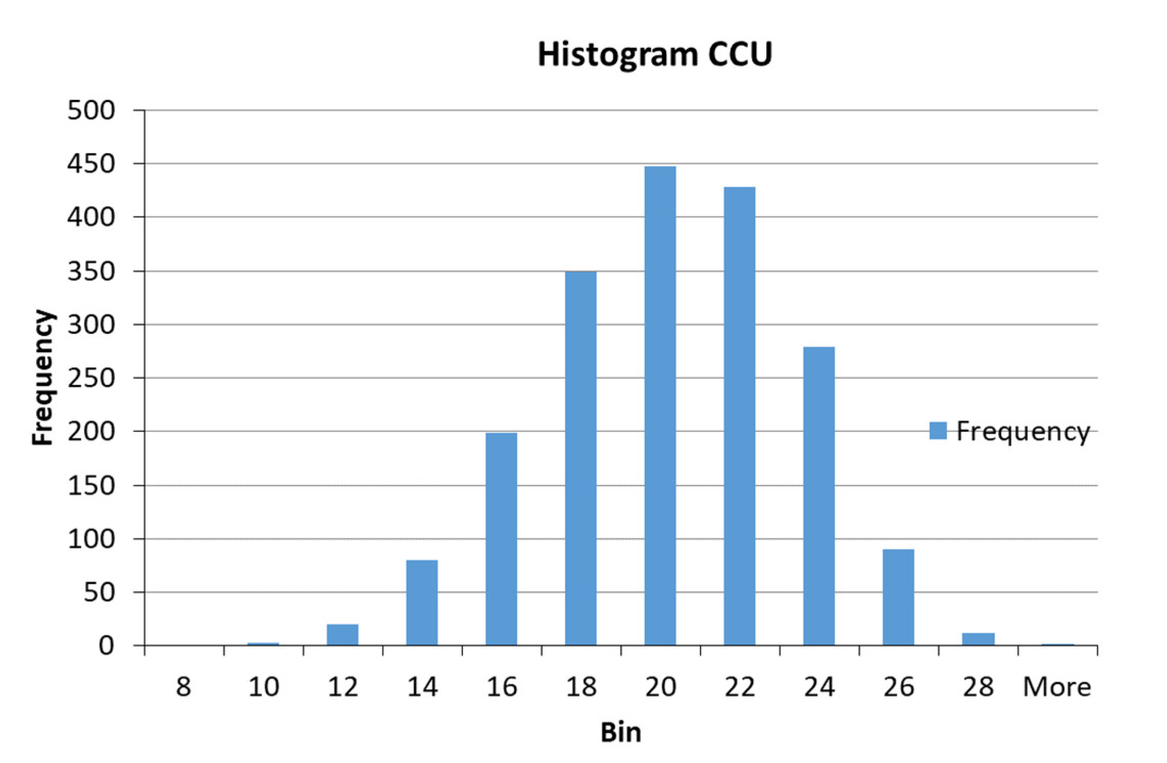
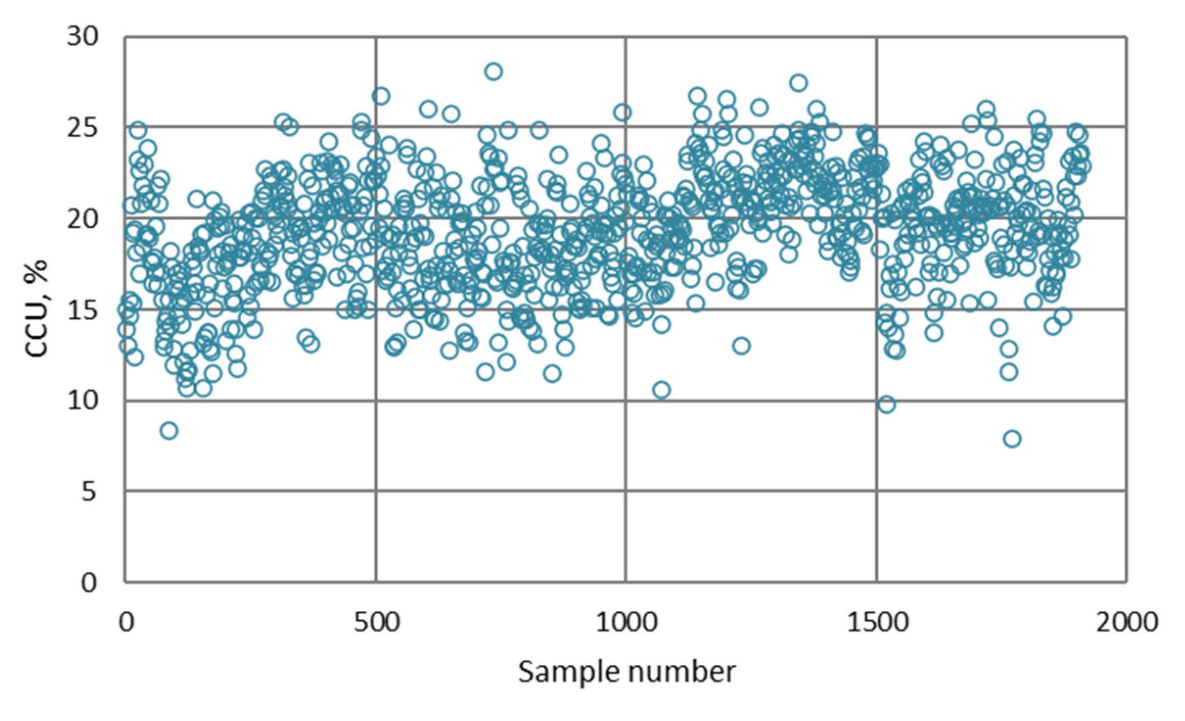
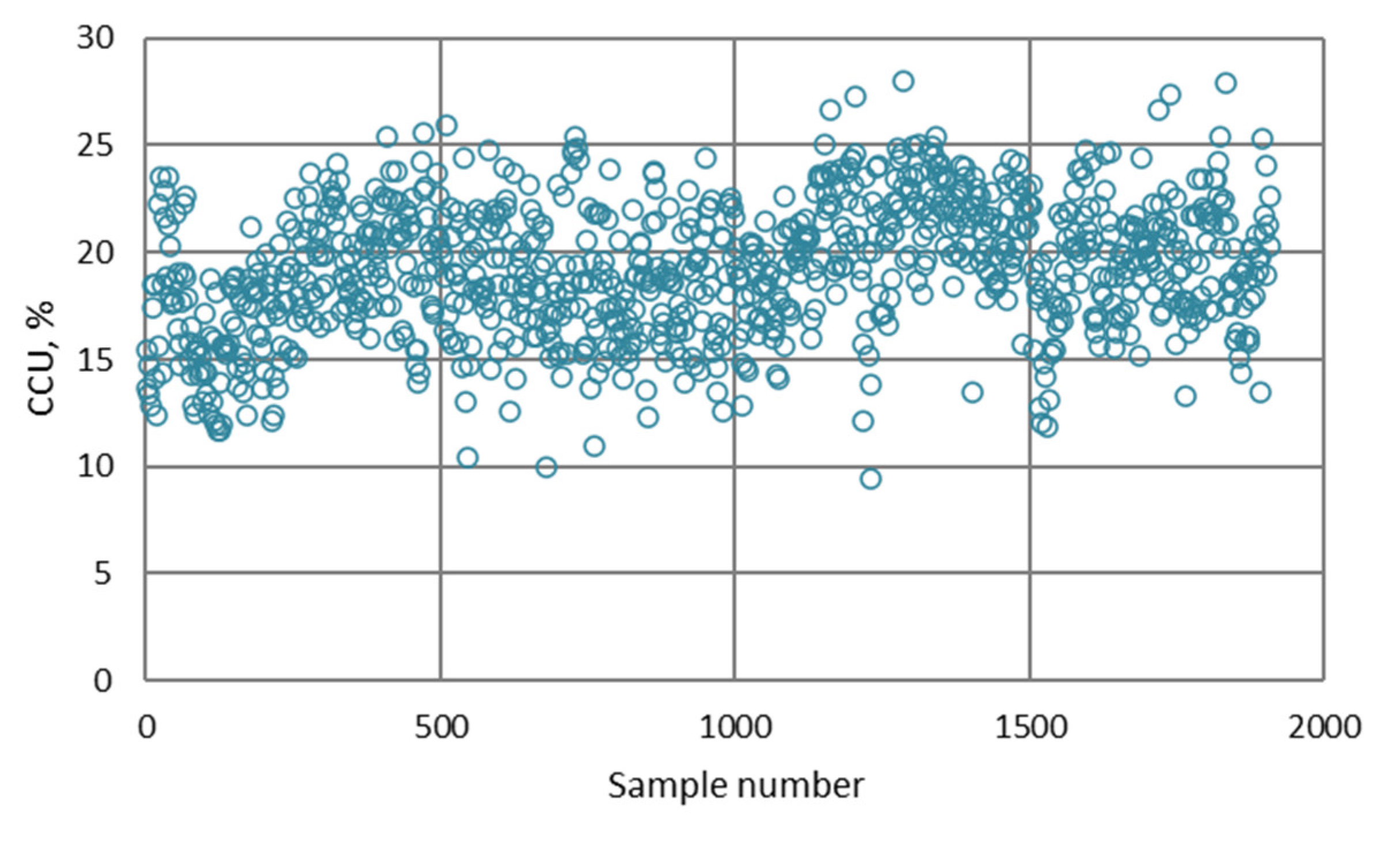
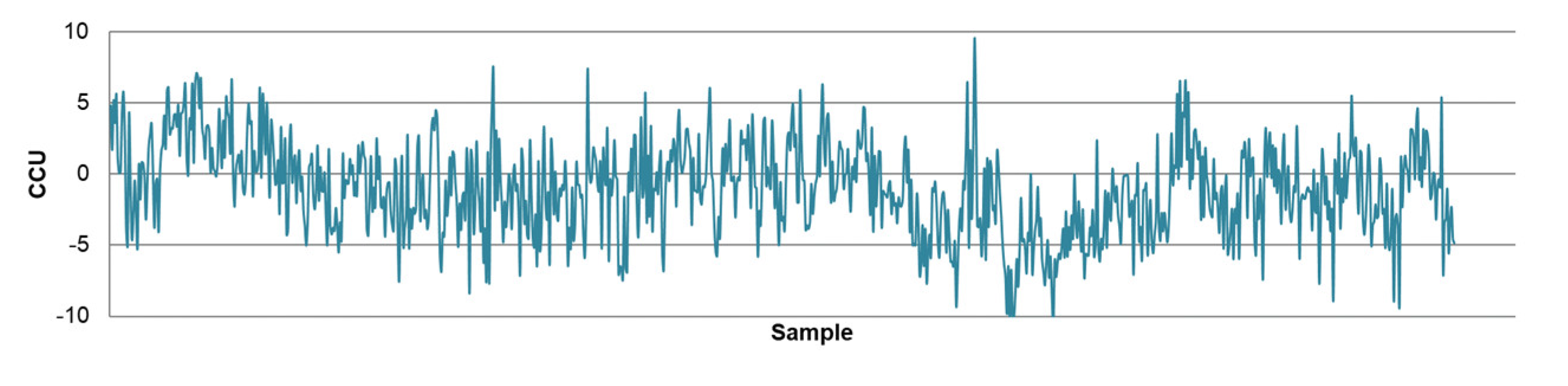
| Copper content in the final concentrate | CCU | % |
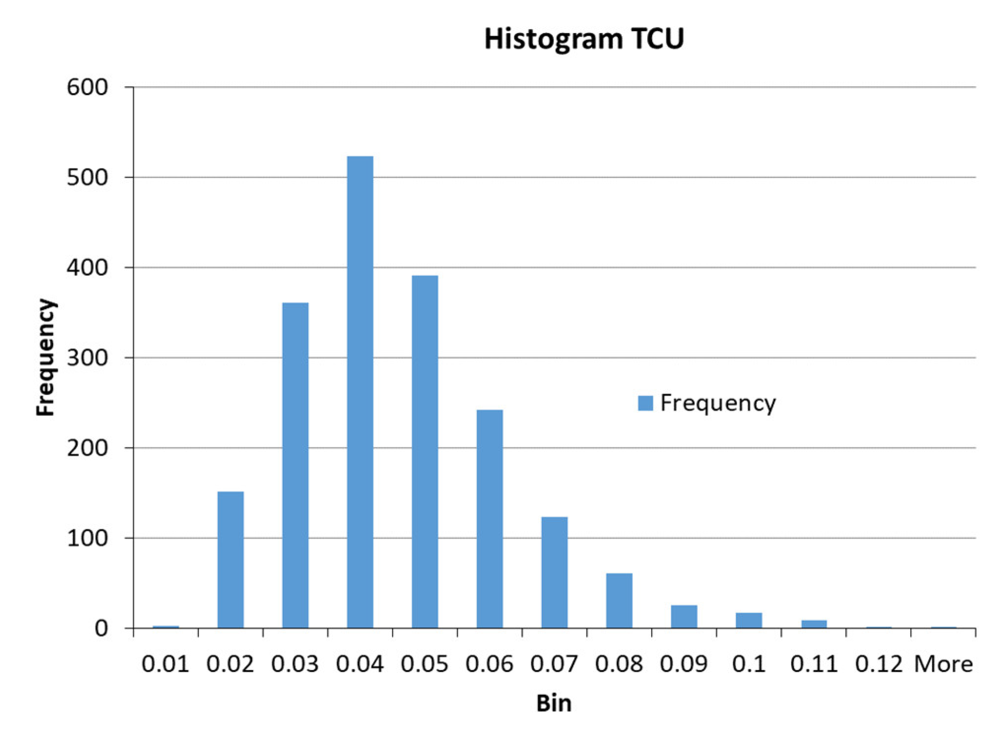
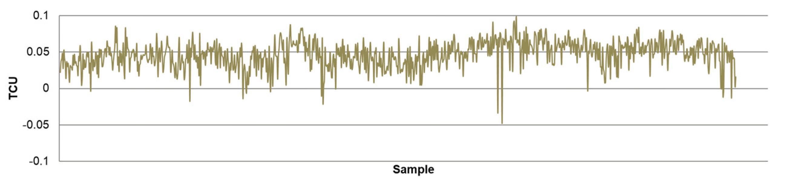
| Copper content in the final tailings | TCU | % |
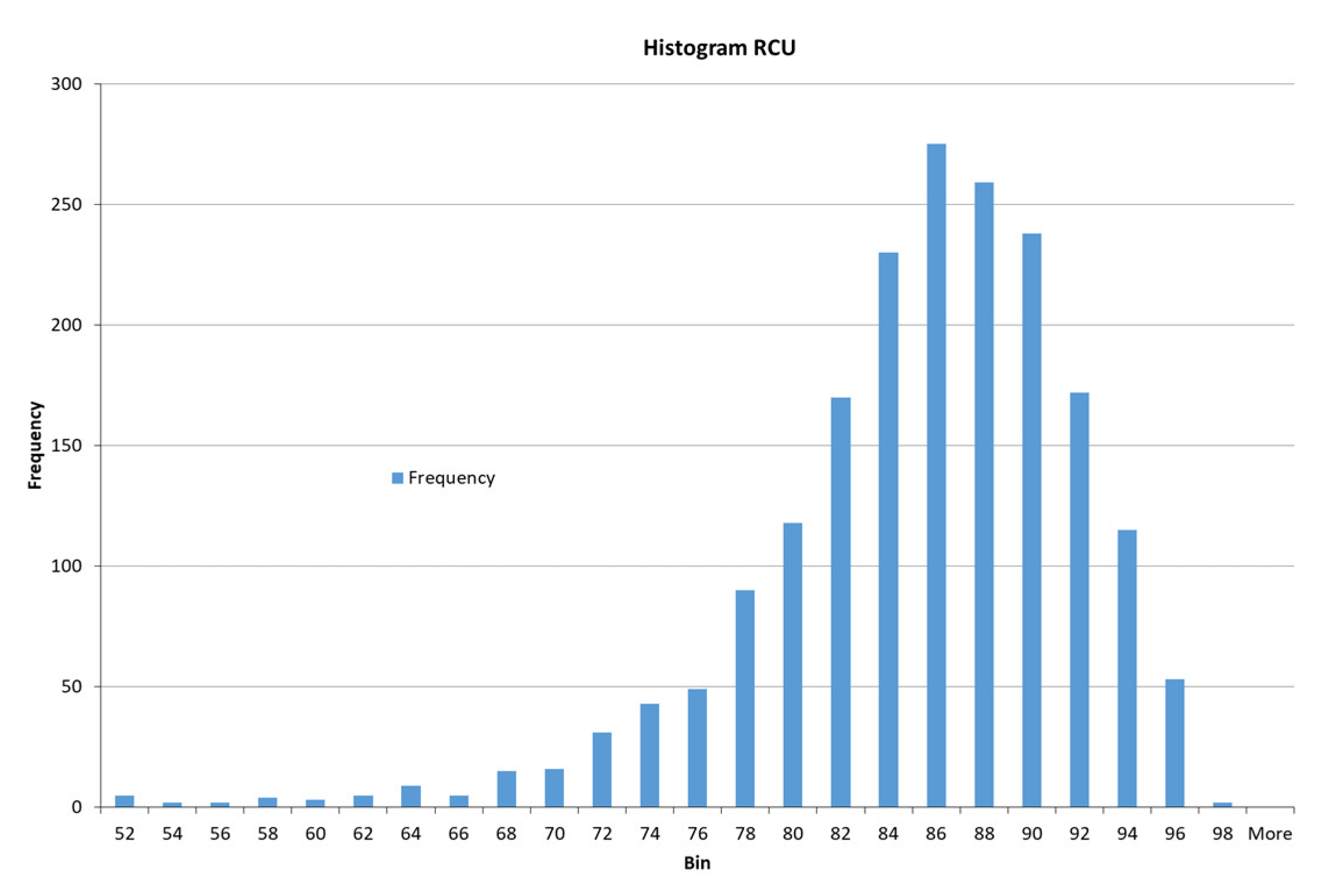
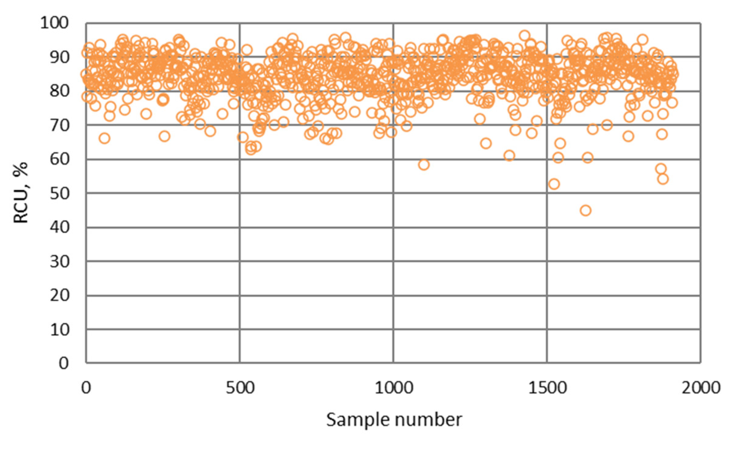
| Copper recovery in the final concentrate | RCU | % |
| Statistical Indicator | Input Variables | Output Variables | ||||||
|---|---|---|---|---|---|---|---|---|
| FCU | PXR | FRT | PHR | PXS | CCU | TCU | RCU | |
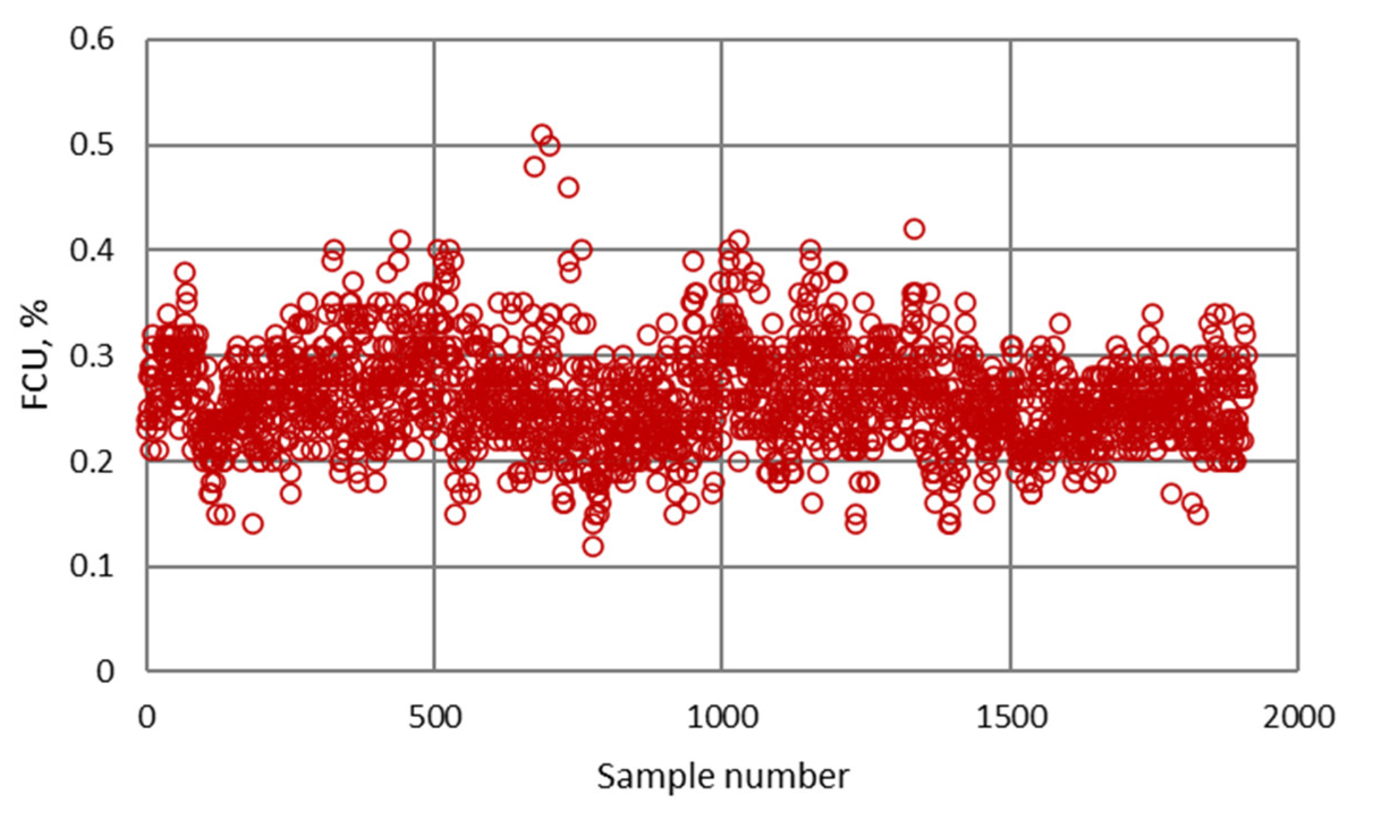
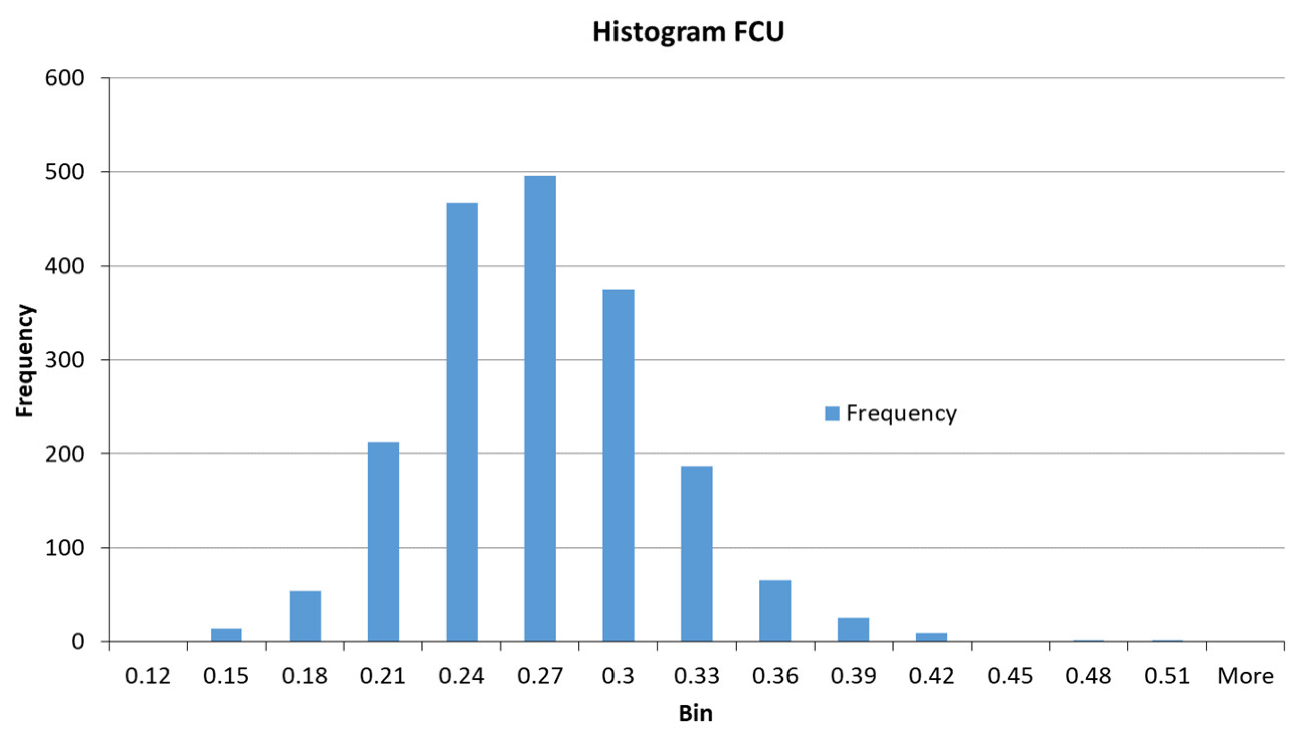
| Minimum | 0.12 | 10.00 | 1.02 | 8.44 | 2.50 | 7.91 | 0.009 | 40.78 |
| Maximum | 0.51 | 49.98 | 16.97 | 11.97 | 7.90 | 28.09 | 0.149 | 96.48 |
| Mean | 0.26 | 32.27 | 6.19 | 10.40 | 5.38 | 19.24 | 0.041 | 84.24 |
| Mod | 0.26 | 33.50 | 3.80 | 9.85 | 5.00 | 18.48 | 0.035 | 90.77 |
| Median | 0.26 | 33.30 | 5.87 | 10.45 | 5.25 | 19.34 | 0.038 | 85.18 |
| Standard deviation | 0.046 | 5.046 | 2.319 | 0.645 | 0.774 | 3.129 | 0.017 | 6.751 |
| Confidence interval | 0.002 | 0.226 | 0.104 | 0.029 | 0.035 | 0.140 | 0.001 | 0.303 |
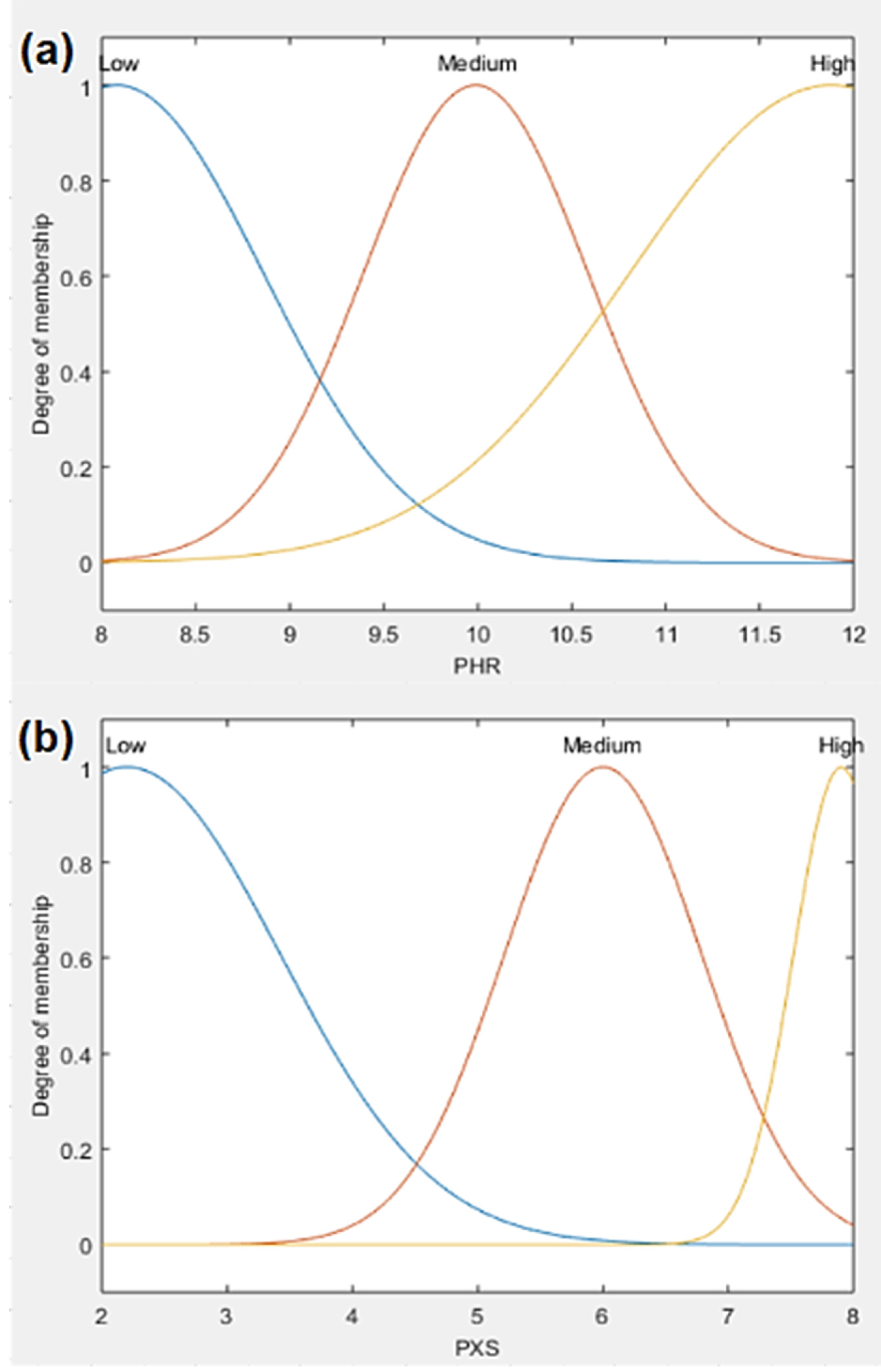
| Variable | Membership Function | Range of Values | Range Fuzzification (Linguistic Value of the Variable) | |
|---|---|---|---|---|
| Input (independent) | FCU | Gaussian | σ/2 = 0.04778; c = 0.112 | Low |
| σ/2 = 0.07976; c = 0.3008 | Medium | |||
| σ/2 = 0.02871; c = 0.492 | High | |||
| PXR | Gaussian | σ/2 = 4.743; c = 10.5 | Low | |
| σ/2 = 6.37; c = 30.0 | Medium | |||
| σ/2 = 4.678; c = 49.0 | High | |||
| FRT | Gaussian | σ/2 = 1.362; c = 0.325 | Low | |
| σ/2 = 1.486; c = 6.5 | Medium | |||
| σ/2 = 5.335; c = 17.4 | High | |||
| PHR | Gaussian | σ/2 = 0.779; c = 8.08 | Low | |
| σ/2 = 0.598; c = 9.989 | Medium | |||
| σ/2 = 1.071; c = 11.88 | High | |||
| PXS | Gaussian | σ/2 = 1.225; c = 2.2 | Low | |
| σ/2 = 0.7887; c = 6.0 | Medium | |||
| σ/2 = 0.3802; c = 7.9 | High | |||
| Output PMM | CCU | Trapezoidal | a = 3.439; b = 6.845; c = 8.015; d = 13.98 | Low |
| a = 10.16; b = 12.36; c = 15.28; d = 21.66 | Medium | |||
| a = 19.78; b = 24.18; c = 25.38; d = 28.08 | High | |||
| RCU | Trapezoidal | a = 34.32; b = 43.92; c = 54.12; d = 65.73 | Low | |
| a = 56.05; b = 71.45; c = 76.15; d = 94.35 | Medium | |||
| a = 61.90; b = 82.32; c = 89.90; d = 100.0 | High | |||
| TCU | Trapezoidal | a = 0.0124; b = 0.0394; c = 0.0461; d = 0.0731 | Low | |
| a = 0.0609; b = 0.0878; c = 0.0946; d = 0.1216 | Medium | |||
| a = 0.1227; b = 0.1497; c = 0.1565; d = 0.1834 | High | |||
| Output PSM | CCU | Constant | z = 8.8 | Low |
| z = 15.08 | Medium | |||
| z = 24.25 | High | |||
| RCU | Constant | z = 49.61 | Low | |
| z = 74.69 | Medium | |||
| z = 83.07 | High | |||
| TCU | Constant | z = 0.0427 | Low | |
| z = 0.0912 | Medium | |||
| z = 0.153 | High | |||
| Independent Variable | Action 1 | ||
|---|---|---|---|
| CCU | RCU | TCU | |
| FCU | ↑ | ↓ | ↑ |
| PXR | ↑ | ↑ | ↓ |
| FRT | ↓ | ↑ | ↓ |
| PHR | ↑ | ↓ | ↑ |
| PXS | ↓ | ↑ | ↓ |
| IF FCU is “low” AND PXR is “high” AND FRT is “medium” AND PHR is “medium” AND PXS is “high” THEN CCU is “medium” AND TCU is “low” AND RCU is “high” |
| IF FCU is “medium” AND PXR is “medium” AND FRT is “high” AND PHR is “low” AND PXS is “medium” THEN CCU is “medium” AND TCU is “medium” AND RCU is “high” |
| IF FCU is “high” AND PXR is “medium” AND FRT is “medium” AND PHR is “high” AND PXS is “low” THEN CCU is “high” AND TCU is “medium” AND RCU is “medium” |
| ⋮ etc. |
| Statistical Parameters | Technological Indicator of the Flotation Process | ||
|---|---|---|---|
| CCU | RCU | TCU | |
| R2 | 0.971 | 0.992 | 0.839 |
| RMSE | 3.126 | 7.007 | 0.034 |
| Mean of prediction error, μ | −0.886 | −2.666 | 0.044 |
| SDE | 3.306 | 7.227 | 0.019 |
| Maximum positive error (maximum) | 10.644 | 36.739 | 0.100 |
| Minimum positive error | 0.00069 | 0.00689 | 0.00015 |
| Minimum negative error | −0.01968 | −0.01318 | −0.00001 |
| Maximum negative error (minimum) | −10.743 | −25.233 | −0.047 |
| Mean of relative prediction error, μr | −0.017 | −0.024 | 1.485 |
| SDEr | 0.190 | 0.098 | 1.238 |
| Statistical Parameters | Technological Indicator of the Flotation Process | ||
|---|---|---|---|
| CCU | RCU | TCU | |
| R2 | 0.970 | 0.993 | 0.847 |
| RMSE | 3.291 | 6.739 | 0.034 |
| Mean of prediction error | −0.288 | −2.008 | 0.046 |
| SDE | 3.374 | 6.915 | 0.018 |
| Maximum positive error (maximum) | 10.961 | 39.619 | 0.091 |
| Minimum positive error | 0.00473 | 0.00232 | 0.00128 |
| Minimum negative error | −0.01028 | −0.01190 | −0.00019 |
| Maximum negative error (minimum) | −10.354 | −17.502 | −0.056 |
| Mean of relative prediction error, μr | 0.015 | −0.0165 | 1.562 |
| SDEr | 0.198 | 0.096 | 1.244 |
| Statistical Parameters | Technological Indicator of the Flotation Process | ||
|---|---|---|---|
| CCU | RCU | TCU | |
| R2 | 0.982 | 0.994 | 0.867 |
| RMSE | 2.567 | 6.284 | 0.015 |
| Mean of prediction error | −0.017 | −0.338 | 0.0015 |
| SDE | 2.589 | 6.323 | 0.016 |
| Maximum positive error (maximum) | 10.933 | 44.501 | 0.043 |
| Minimum positive error | 0.00102 | 0.00694 | 0.000003 |
| Minimum negative error | −0.00230 | −0.01246 | −0.00004 |
| Maximum negative error (minimum) | −10.892 | −16.341 | −0.113 |
| Mean of relative prediction error, μr | 0.019 | 0.002 | 0.222 |
| SDEr | 0.154 | 0.089 | 0.551 |
Publisher’s Note: MDPI stays neutral with regard to jurisdictional claims in published maps and institutional affiliations. |
© 2022 by the authors. Licensee MDPI, Basel, Switzerland. This article is an open access article distributed under the terms and conditions of the Creative Commons Attribution (CC BY) license (https://creativecommons.org/licenses/by/4.0/).
Share and Cite
Jovanović, I.; Nakhaei, F.; Kržanović, D.; Conić, V.; Urošević, D. Comparison of Fuzzy and Neural Network Computing Techniques for Performance Prediction of an Industrial Copper Flotation Circuit. Minerals 2022, 12, 1493. https://doi.org/10.3390/min12121493
Jovanović I, Nakhaei F, Kržanović D, Conić V, Urošević D. Comparison of Fuzzy and Neural Network Computing Techniques for Performance Prediction of an Industrial Copper Flotation Circuit. Minerals. 2022; 12(12):1493. https://doi.org/10.3390/min12121493
Chicago/Turabian StyleJovanović, Ivana, Fardis Nakhaei, Daniel Kržanović, Vesna Conić, and Daniela Urošević. 2022. "Comparison of Fuzzy and Neural Network Computing Techniques for Performance Prediction of an Industrial Copper Flotation Circuit" Minerals 12, no. 12: 1493. https://doi.org/10.3390/min12121493