
Aspects of Estimation and Reporting of Mineral Resources of Seabed Polymetallic Nodules: A Contemporaneous Case Study

Abstract
:1. Introduction
1.1. Mineral Owners
1.2. Mineral Developers
1.3. Reporting Rules
- Materiality;
- Transparency;
- Competence and responsibility.
2. History of Evaluation of Polymetallic Nodule Deposits
3. Reporting Standards and the International Seabed Authority
4. Methods for the Evaluation of Polymetallic Nodule Deposits
4.1. Contrasting Estimation of Terrestrial Mineral Resources and Polymetallic Nodule Mineral Resources
4.2. Geology of Polymetallic Nodule Deposits
4.3. Sampling
4.3.1. Physical Sampling
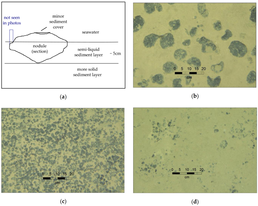
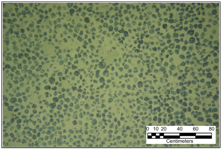
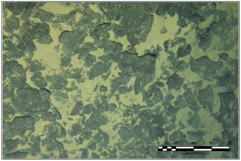
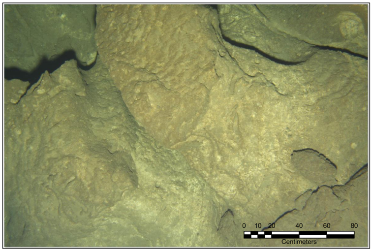
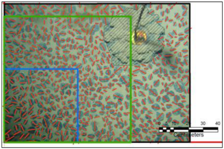
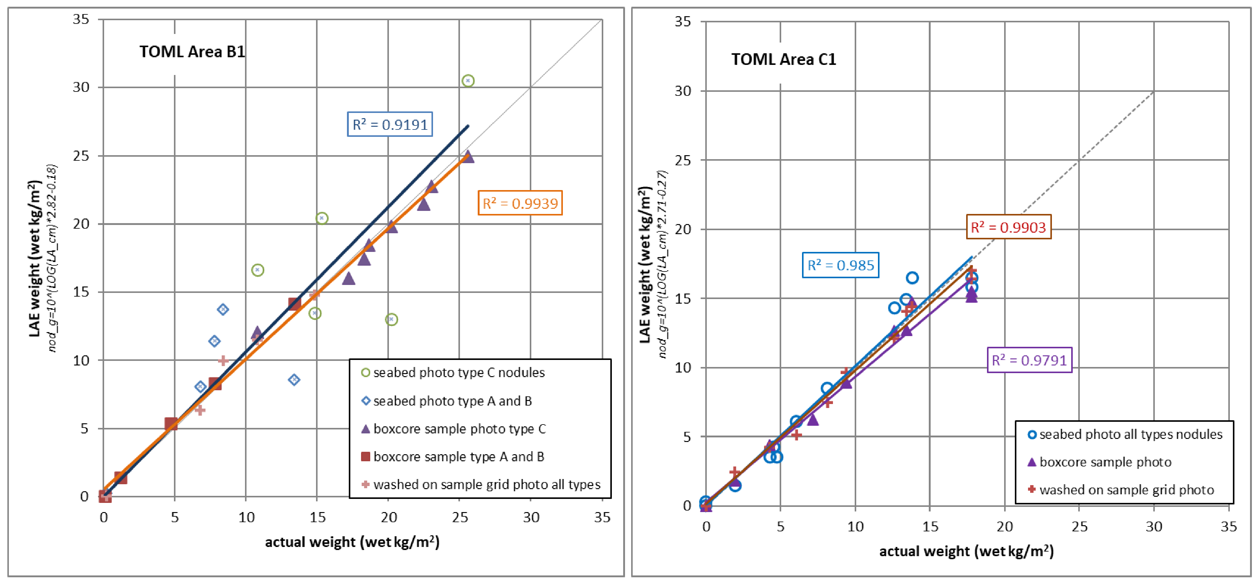
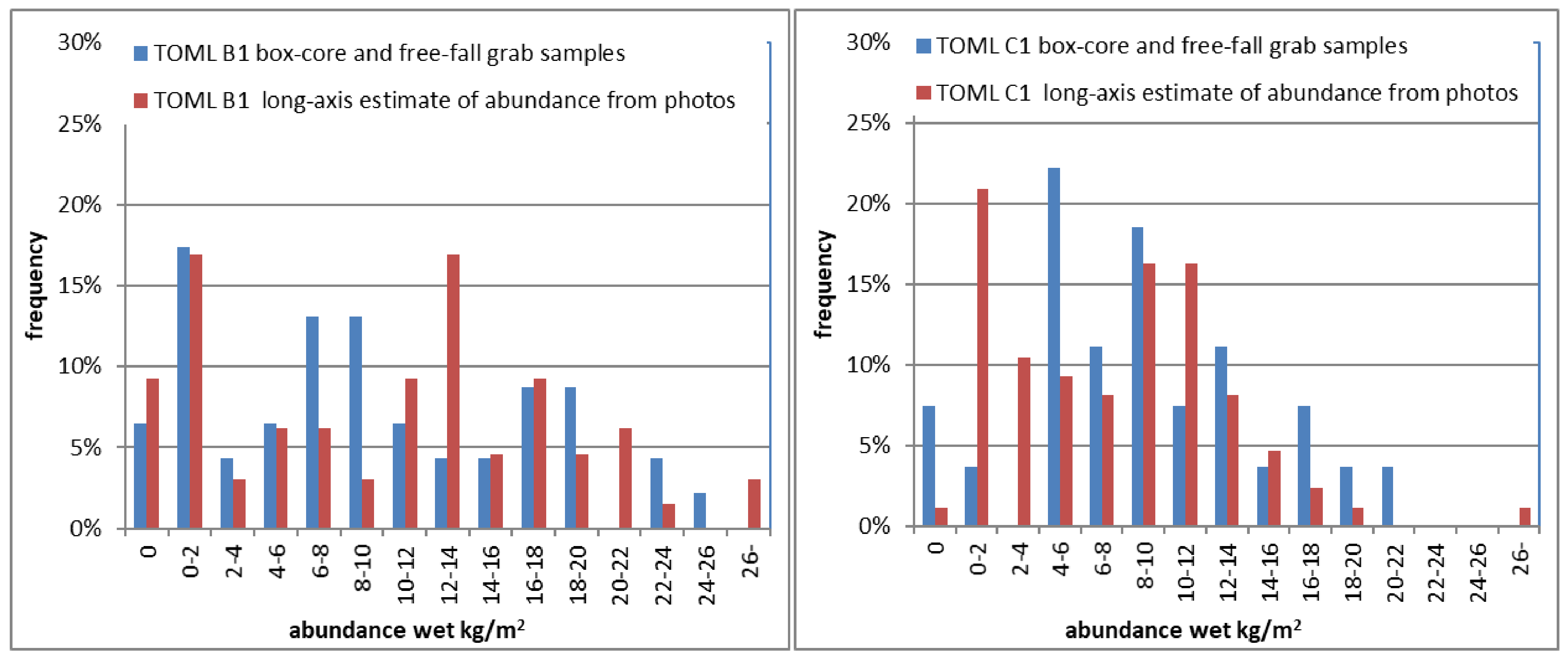
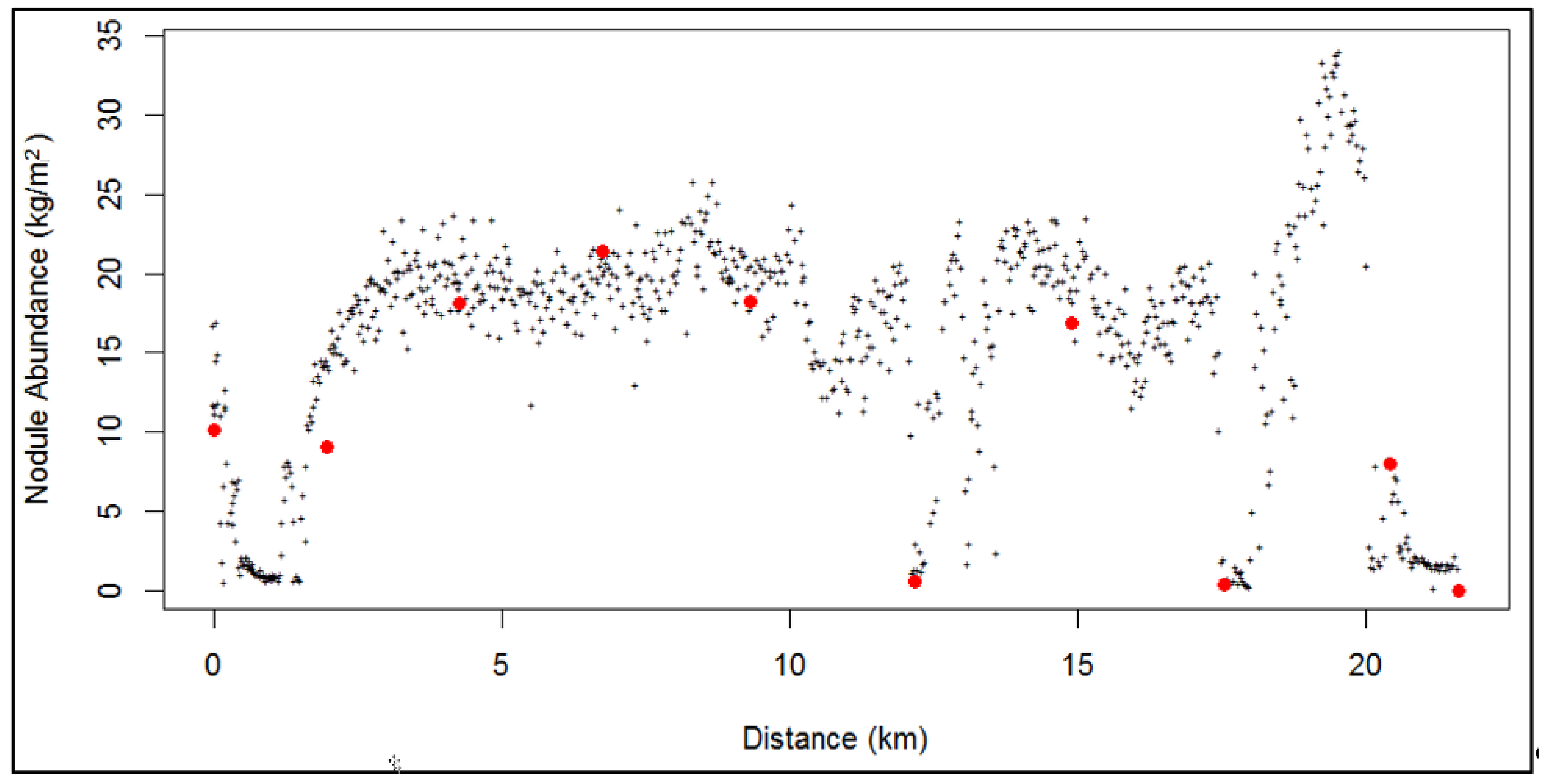
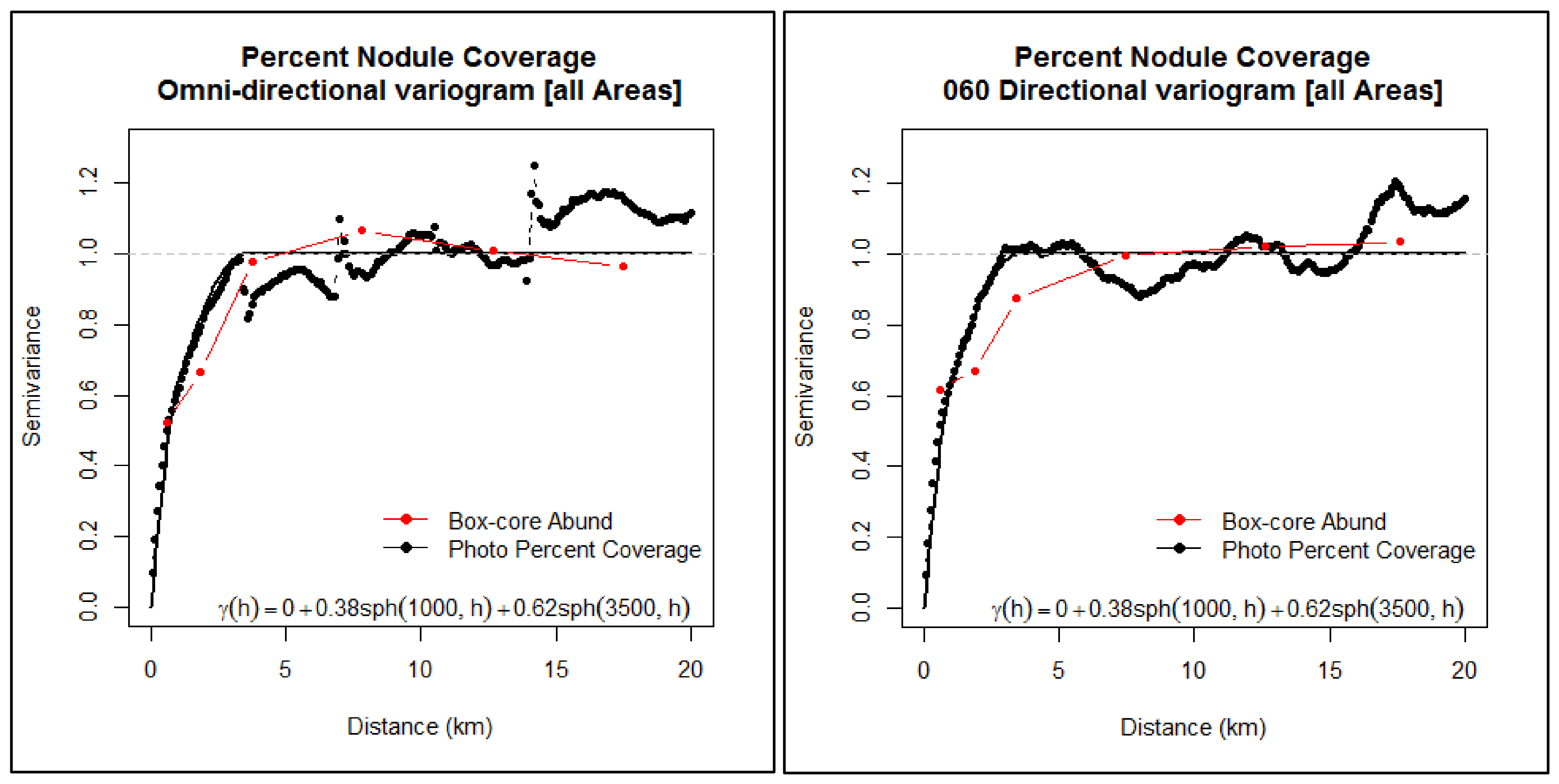
4.3.2. Seafloor Photographs and Long-Axis Estimates of Abundance
- Site-scale variations in the local regression relationships (mostly likely due to site-based variations in the thickness of the geochemically active layer and thus the thickness of the nodules);
- Varying scales in the towed photo images (e.g., a slightly oblique perspective when taking the photograph due to flaring of the towed systems resulting from vessel heave);
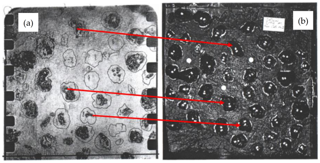
- Partial sediment cloaking or covering of the edges of nodules (Figure 5);
- Imprecision in the manual digitising process.
4.3.3. Assaying
- Split the nodules into representative aliquots;
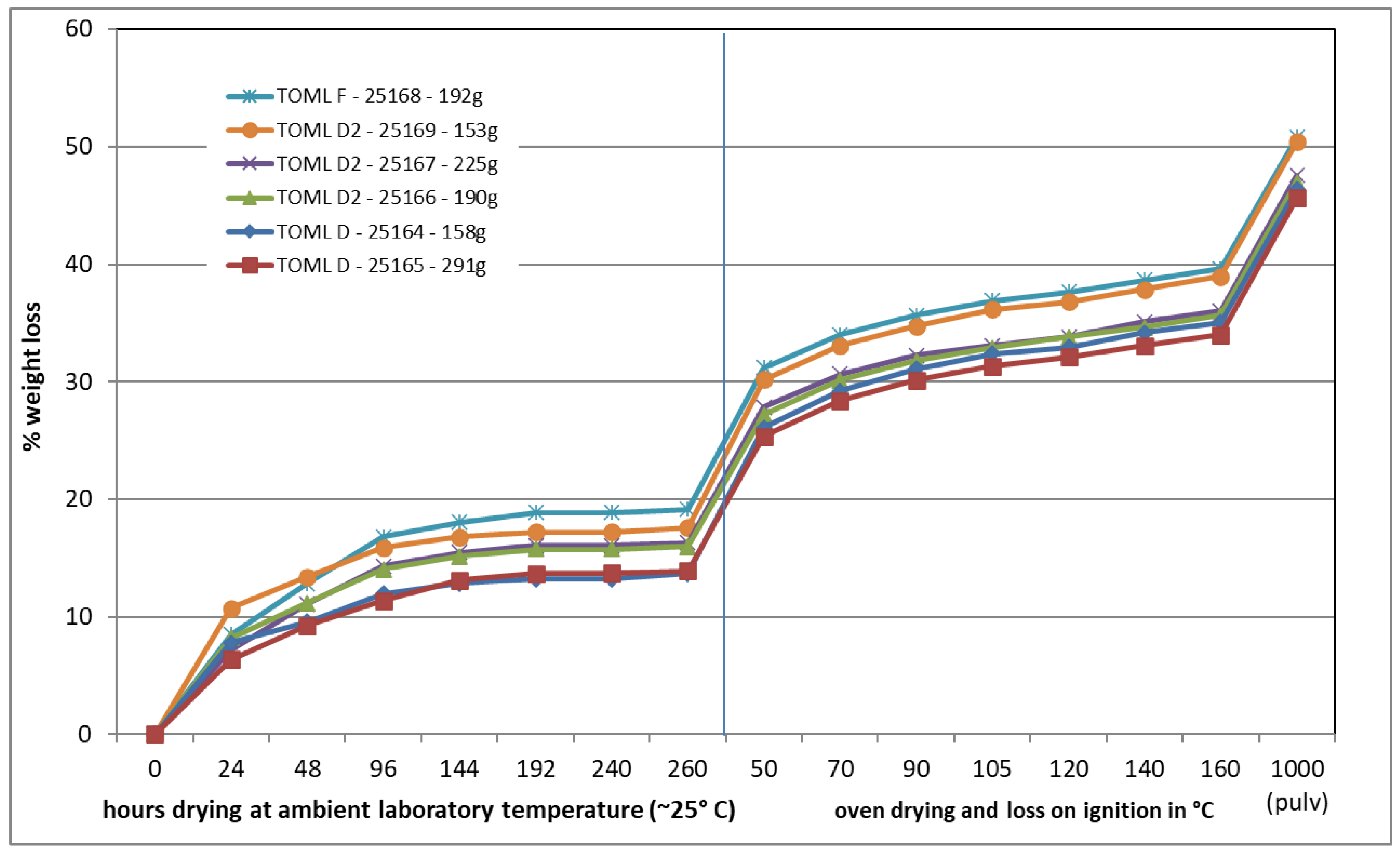
- Dry the nodules and then crush and pulverise them, reducing the sample size between each step with splitters;
- Analyse a wide range of elements using a mixture of X-ray fluorescence (XRF) and inductively coupled plasma spectrometric (ICP) methods. Measure loss on ignition using a thermogravimetric analysis furnace;
- Use blanks, duplicates, and certified reference materials not known to the laboratory to confirm the precision and accuracy of the analyses.
- Water of crystallisation included within the manganese and iron oxide minerals. This was determined in TOML test work to consistently be around 16% by wet weight (including the likely trace levels of other volatiles) [12]. A very small amount of water from crystallisation likely starts to be removed at temperatures as low as 50–70 °C through a transformation of the manganese mineral buserite into birnessite, but most manganese and iron oxide minerals are stable until reaching higher temperatures (115 °C and greater; Novikov and Bogdanova [71]);
- Free water included within pores and other cavities within the nodules, including water adsorbed onto mineral surfaces—this is estimated to be around 28% by wet weight depending on the micro and macro void space in the nodules. Air-drying may remove approximately 16% (absolute) of this, with the rest removed by oven drying (up to 105 °C).
4.3.4. Historical Samples
- Corroborate the ISA-supplied historical results by comparing the data between different original collection organisations and with other published data (non-ISA) from the CCZ nodule deposit. This was possible due to the large size of the CCZ deposit and the relative homogeneity of the grades across vast areas.
- Demonstrate a level of quality control by directly requesting information on sample collection and analysis from the original groups, also noting that the ISA, as an independent and accountable organisation, would need to check the data they received, as these data were used to define retained and released mineral rights under the groups’ administration.
- Retain the services of an independent qualified person with direct experience in sample collection from the CCZ.
5. Estimation Case Study—Tonga Offshore Mining Limited Contract Area
5.1. Samples and Related Data
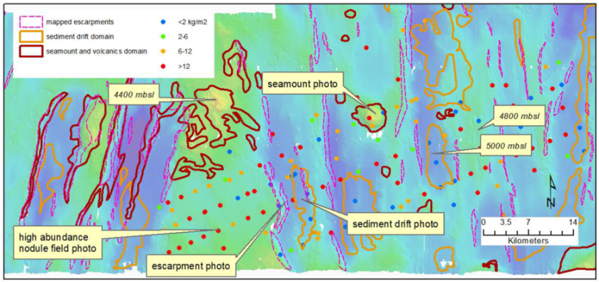
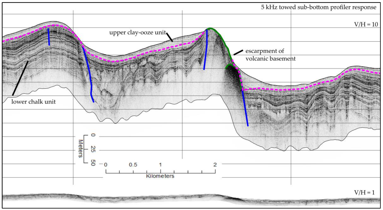
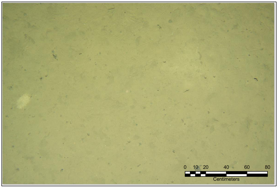
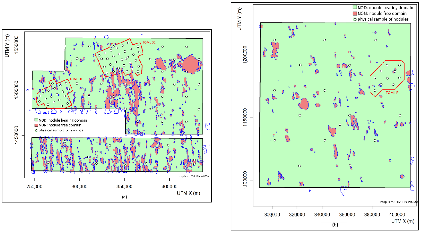
5.2. Domains and Model
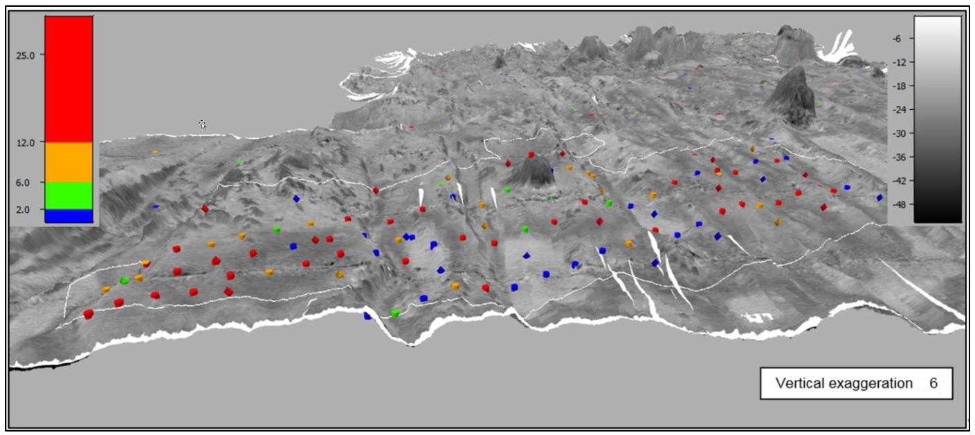
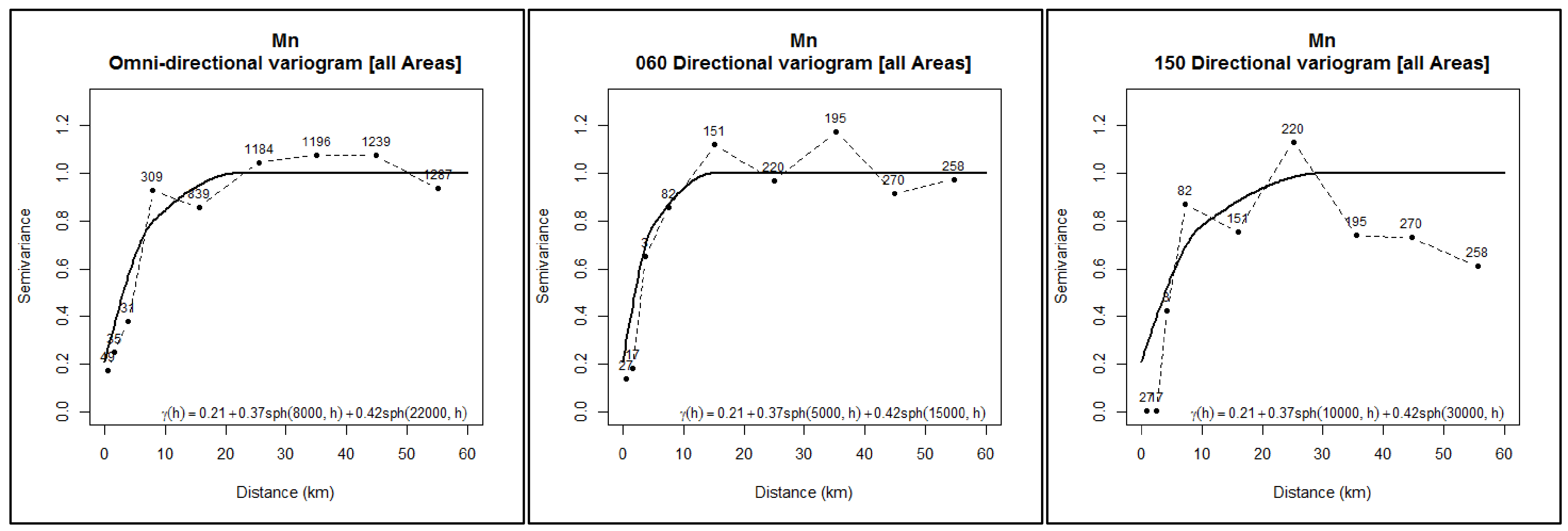
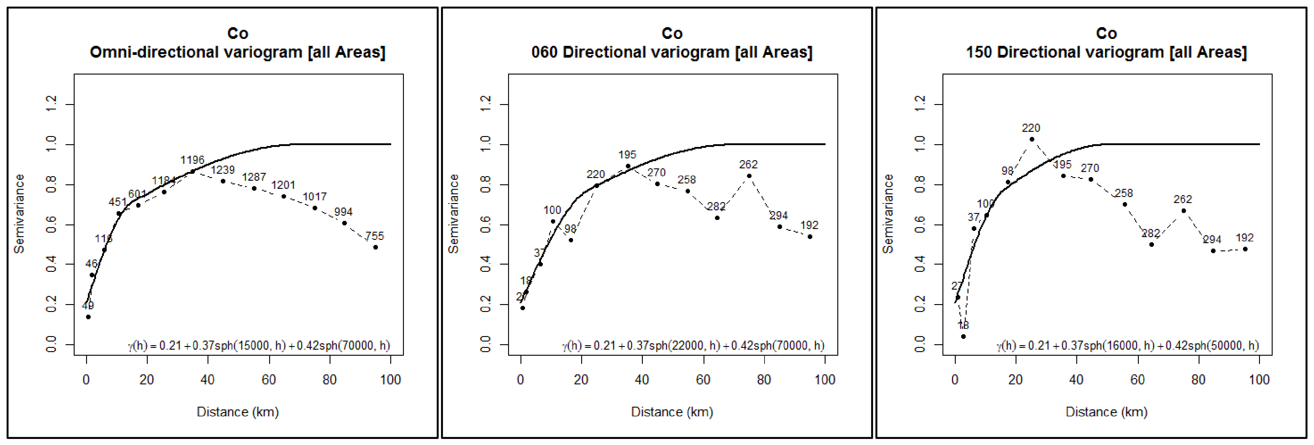
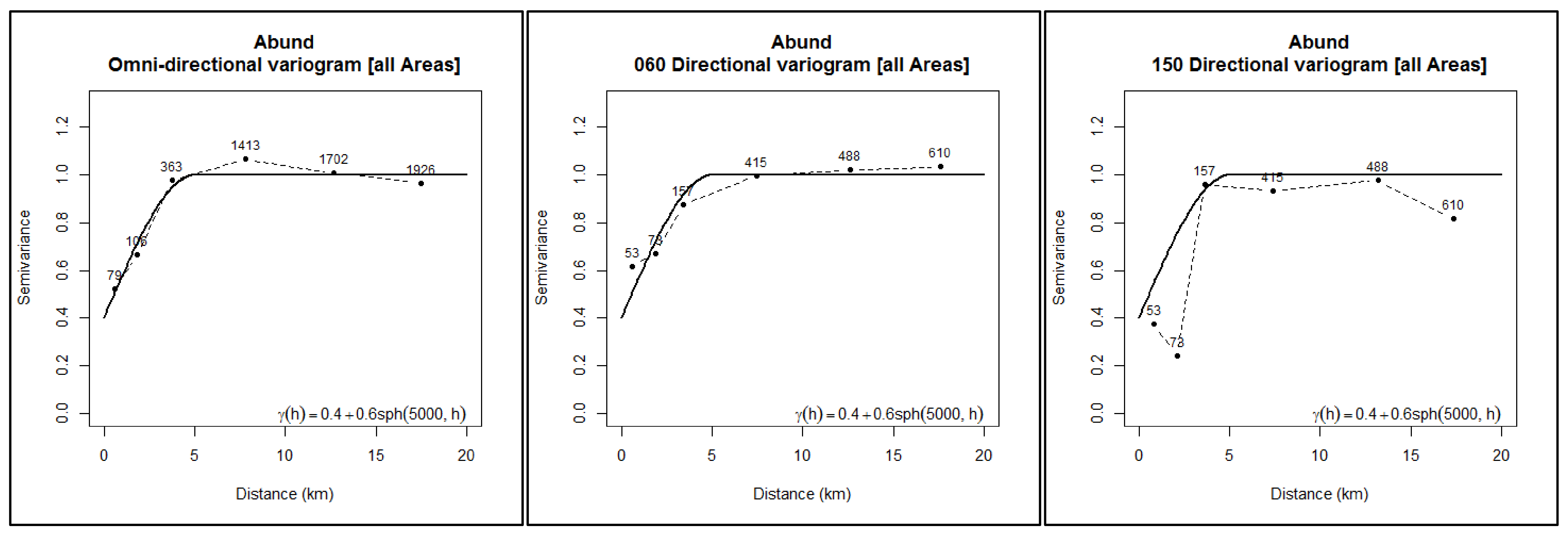
5.3. Geostatistics and Model Estimation
6. Discussion
6.1. Reasonable Prospects of Eventual Economic Extraction
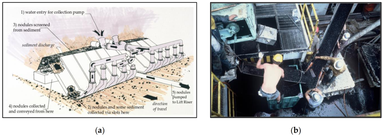
- In the foreseeable future, mining of polymetallic nodules from the seafloor would be technically feasible.
- Processing of polymetallic nodules to extract nickel copper, cobalt, and manganese products would likely be feasible using a combination of existing extractive technologies (e.g., Haynes et al. [74]).
- The metal products would have a market because there is anticipated to be increasing demand for these metals for traditional purposes supported by increased demand for electrochemical cells (batteries).
- The entire process, from seafloor collection to the delivery of metalliferous products, could be achieved in an economically viable manner.
- Success in the pilot mining of polymetallic nodules in the CCZ by two groups in the late 1970s (e.g., Brockett et al. [51]).
- Successful sub-sea operations at similar or greater water depths, including tasks such as the installation of oil and gas production facilities at circa 2500 m; the spudding of drill holes at circa 3000 m; cable laying and retrieval at circa 5000 m; and the collection of samples at circa 11,000 m.
- Demonstration of various lift systems from water depths such as the CCZ, including cable, pumping, and airlift solutions.
- Demonstration of operating offshore production vessels including the transfer of product.
- The similarities of some proposed metallurgical processing routes to existing facilities for terrestrial ore sources.
- Higher grades than some terrestrial ore sources and upsides in terms of recoverable metals.
- Lack of overburden and no need to cut rock, at least in part, compensating for working at a depth. Reduced mine infrastructure outside of the production system.
- Transport distances for product comparable with those of other seaborne bulk commodities.
- Benefits of homogenous mineralogy in metallurgical optimisation and cost reduction.
6.2. Marine Environment
6.3. Qualified Persons, Independence, and Transparency
6.4. Property Inspection and Chain Of Custody
- The inclusion of a QP who had actually spent 3 months working in the CCZ;
- A documented chain of custody around the collection of box core samples and seafloor images; and
- The fact that numerous other independent organisations had explored the deposit in the past and reported essentially similar results.
7. Conclusions
Author Contributions
Funding
Institutional Review Board Statement
Informed Consent Statement
Data Availability Statement
Acknowledgments
Conflicts of Interest
References
- International Seabed Authority. Establishment of a geological model of the polymetallic nodule resources in the Clarion-Clipperton Fracture Zone of the Equatorial North Pacific Ocean. In Proceedings of the International Seabed Authority workshop, Nadi, Fiji, 13–20 May 2003. [Google Scholar]
- Mukhopadhyay, R.; Chosh, A.K.; Iyer, S.D. The Indian Ocean Nodule Field—Geology and Resource Potential, 2nd ed.; Elsevier: Amsterdam, The Netherlands, 2018; ISBN 978-0-12-805474-1. [Google Scholar]
- Watzel, R.; Rühlemann, C.; Vink, A. Mining mineral resources from the seabed: Opportunities and challenges. Mar. Policy 2020, 114, 103828. [Google Scholar] [CrossRef]
- Toro, N.; Robles, P.; Jeldres, R.I. Seabed mineral resources, an alternative for the future of renewable energy: A critical review. Ore Geol. Rev. 2020, 126, 103699. [Google Scholar] [CrossRef]
- Hein, J.R.; Koschinsky, A.; Kuhn, T. Deep-ocean polymetallic nodules as a resource for critical materials. Nat. Rev. Earth Environ. 2020, 1, 158–169. [Google Scholar] [CrossRef]
- Andreev, S.; Burskey, A.Z.; Gramberg, I.S.; Anikeeva, I.I.; Ivanova, A.M.; Kotlinski, R.; Zadornov, M.M.; Miletenki, N.V.; Mirchink, I.M. Metallogenic Map of the World Ocean, 2nd ed.; Andreev, S., Ed.; Vniiokeangeologia: St Petersburg, Russia, 2008. [Google Scholar]
- Matthews, K.J.; Müller, R.D.; Wessel, P.; Whittaker, J.M. The tectonic fabric of the ocean basins. J. Geophys. Res. 2011, 116, B12109. [Google Scholar] [CrossRef] [Green Version]
- United Nations Division for Ocean Affairs and the Law of the Sea. The United Nations Convention on the Law of the Sea (A historical perspective 1998). Available online: https://www.un.org/Depts/los/convention_agreements/convention_historical_perspective.htm (accessed on 20 December 2020).
- International Seabed Authority. The Law of the Sea—Compendium of Basic Documents; Authority, I.S., Ed.; International Seabed Authority: Kingston, Jamaica; United Nations: New York, NY, USA, 2001; ISBN 976-610-374-7. [Google Scholar]
- Madureira, P.; Brekke, H.; Cherkashov, G.; Rovere, M. Exploration of polymetallic nodules in the Area: Reporting practices, data management and transparency. Mar. Policy 2016, 70, 101–107. [Google Scholar] [CrossRef] [Green Version]
- National Oceanic and Atmospheric Administration Seabed Management. Available online: http://www.gc.noaa.gov/gcil_seabed_management.html (accessed on 4 April 2016).
- Lipton, I.; Nimmo, M.; Parianos, J. TOML Clarion Clipperton Zone Project, Pacific Ocean; AMC Consultants Pty Ltd.: Brisbane, Australia, 2016. [Google Scholar]
- International Seabed Authority. Available online: www.isa.org.jm (accessed on 19 July 2020).
- Sparenberg, O. A historical perspective on deep-sea mining for manganese nodules, 1965–2019. Extr. Ind. Soc. 2019, 6, 842–854. [Google Scholar] [CrossRef]
- Marine Regions Martime Boundaries v11. 2019. Available online: https://marineregions.org/downloads.php (accessed on 5 October 2020).
- Committee for Mineral Reserves International Reporting Standards Committee for Mineral Reserves International Reporting Standards (CRIRSCO). Available online: http://www.crirsco.com/background.asp (accessed on 19 July 2020).
- Joint Ore Reserves Committee. The Australasian Code for Reporting of Exploration Results, Mineral Resources and Ore Reserves—The JORC Code; The Australasian Institute of Mining and Metallurgy, Australian Institute of Geoscientists and Minerals Council of Australia: Carlton, Australia, 2012. [Google Scholar]
- CIM. CIM Definitions Standards—For Mineral Resources and Mineral Reserves; Canadian Institute of Mining, Metallurgy and Petroleum: Westmount, QC, Canada, 2010. [Google Scholar]
- CIM. CIM Definition Standards—For Mineral Resources and Mineral Reserves; Canadian Institute of Mining, Metallurgy and Petroleum: Westmount, QC, Canada, 2014. [Google Scholar]
- CIM Mineral Resource & Mineral Reserve Committee. CIM Estimation of Mineral Resources & Mineral Reserves Best Practice Guidelines; Canadian Institute of Mining, Metallurgy and Petroleum: Westmount, QC, Canada, 2019. [Google Scholar]
- Committee for Mineral Reserves International Reporting Standards (CRIRSCO). International Reporting Template for the Public Reporting of Exploration Targets, Exploration Results, Mineral Resources and Mineral Reserves; Committee for Mineral Reserves International Reporting Standards (CRIRSCO): Clayton, Australia, 2019. [Google Scholar]
- Nimmo, M.; Morgan, C.; Banning, D. Clarion-Clipperton Zone Project, Pacific Ocean; Golder Associates Ltd.: Brisbane, Australia, 2013. [Google Scholar]
- DeWolfe, J.; Ling, P. NI 43-101 Technical Report for the NORI Clarion - Clipperton Zone Project, Pacific Ocean; Golder Associates Ltd.: Vancouver, Canada, 2018. [Google Scholar]
- Lipton, I.; Nimmo, M.; Stevenson, I. NORI Area D Clarion Clipperton Zone Mineral Resource Estimate; AMC Consultants Pty Ltd.: Brisbane, Australia, 2019. [Google Scholar]
- Lipton, I.; Nimmo, M.; Stevenson, I. NORI Area D Clarion Clipperton Zone Mineral Resource Estimate—Update; AMC Consultants Pty Ltd.: Brisbane, Australia, 2021. [Google Scholar]
- Murray, J.; Renard, A.F. Deep-Sea Deposits (Based on the Specimens Collected during the Voyage of HMS Challenger in the Years 1872 to 1876); Eyre and Spottiswoode: London, UK, 1891. [Google Scholar]
- Menard, H.W.; Shipek, C.J. Surface Concentrations of Manganese Nodules. Nature 1958, 182, 1156–1158. [Google Scholar] [CrossRef]
- Mero, J. The Mineral Resources of the Sea; Elsevier Oceanography Series: Amsterdam, Holland, 1965. [Google Scholar]
- United Nations Ocean Economics and Technology Branch. Assessment of Manganese Nodule Resources, 1st ed.; Graham and Trotman: London, UK, 1982; ISBN 0860103471. [Google Scholar]
- Pasho, D.W.; McIntosh, J. Recoverable nickel and copper from manganese nodules in the northeast equatorial Pacific—Preliminary results. Can. Inst. Min. Metall. Bull. 1976, 69, 15. [Google Scholar]
- Bastien-Thiry, H.; Lenoble, J.-P.; Rogel, P. French exploration seeks to define minable nodule tonnages on Pacific floor. Eng. Min. J. 1977, 171, 86–87. [Google Scholar]
- McKelvey, V.E.; Wright, N.A.; Rowland, R. Manganese nodule resources in the northeastern equatorial Pacific. In Marine Geology and Oceanography of the Pacific Manganese Nodule Province; Bishoff, J.L., Piper, D.Z., Eds.; Plenum: New York, NY, USA, 1979. [Google Scholar]
- Lenoble, J.-P. Polymetallic nodules resources and reserves in the North Pacific from the data collected by AFERNOD. Ocean Manag. 1981, 7, 9–24. [Google Scholar] [CrossRef]
- Kotlinski, R.; Zadornov, M. Peculiarities of nodule ore potential of the eastern part of the Clarion-Clipperton field (prospecting area of Interoceanmetal). In Proceedings of the Minerals of the Ocean; Ministry of Natural Resources, Russian Academy of Sciences, St. Petersburg, Russia, 23 December 2002; pp. 21–24. [Google Scholar]
- De Souza, K. International Seabed Authority’s resource assessment of the metals found in polymetallic nodule deposits in the Area. In Establishment of a Geological Model of Polymetallic Nodule Deposits in the Clarion-Clipperton Fracture Zone of the Equatorial North Pacific Ocean, Proceedings of the International Seabed Authority workshop, Nadi, Fiji, 13–20 May 2003; Office of Resources and Environmental Monitoring, Ed.; International Seabed Authority: Kingston, Jamaica, 2003; pp. 28–41. [Google Scholar]
- De L’Etoile, R. Geostatistical analysis and evaluation of the metals contained in polymetallic nodules in reserved areas. In The Geological Model of Polymetallic Nodule Deposits in the Clarion-Clipperton Fracture Zone of the Equatorial North Pacific Ocean, Proceedings of the International Seabed Authority workshop, Nadi, Fiji, 13–20 May 2003; Office of Resources and Environmental Monitoring, Ed.; International Seabed Authority: Kingston, Jamaica, 2003; pp. 42–69. [Google Scholar]
- Morgan, C. Proposed model data inputs. In the Geological Model of Polymetallic Nodule Deposits in the Clarion-Clipperton Fracture Zone of the Equatorial North Pacific Ocean, Proceedings of the International Seabed Authority workshop, Nadi, Fiji, 13–20 May 2003; Office of Resources and Environmental Monitoring, Ed.; International Seabed Authority: Kingston, Jamaica, 2003; pp. 80–95. [Google Scholar]
- International Seabed Authority. A Geological Model of Polymetallic Nodule Deposits in the Clarion-Clipperton Fracture Zone; International Seabed Authority: Kingston, Jamaica, 2010. [Google Scholar]
- Ruhlemann, C.; Kuhn, T.; Wiedicke, M.; Kasten, S.; Mewes, K.; Picard, A. Current status of manganese nodule exploration in the German licence area. In Proceedings of the Ninth (2011) ISOPE Ocean Mining Symposium, Maui, HI, USA, 19–24 June 2011; pp. 19–24. [Google Scholar]
- International Seabed Authority. Outcomes of the international workshop on polymetallic nodule resource classification held in Goa, India, from 13 to 17 October 2014. Available online: https://www.isa.org.jm/sites/default/files/files/documents/isba-21ltc-7_1.pdf (accessed on 15 December 2020).
- International Seabed Authority. Polymetallic Nodule Resource Classification Workshop. Briefing Paper 01/2016; International Seabed Authority: Kingston, Jamaica, 2016. [Google Scholar]
- State Scientific Center Yuzhmorgeologia. The concept of the Russian exploration area polymetallic nodules resource and reserve categorization. In Polymetallic Nodule Resources Classification, Proceedings of the International Seabed Authority and Ministry of Earth Sciences, Government of India Workshop, Goa, India, 13–17 October 2014; International Seabed Authority: Kingston, Jamaica, 2014. [Google Scholar]
- Korea Institute of Ocean Science and Technology Status of Korea Activities in Resource Assessment and Mining Technologies. Polymetallic Nodule Resources Classification; International Seabed Authority: Kingston, Jamaica, 2014. [Google Scholar]
- Deep Ocean Resources Development Co., Ltd. Polymetallic Nodule Resources Evaluation—How we are doing. In Proceedings of the Workshop on Polymetallic Nodule Resources Classification, Proceedings of the International Seabed Authority and Ministry of Earth Sciences, Government of India Workshop, Goa, India, 13–17 October 2014; International Seabed Authority: Kingston, Jamaica, 2014. [Google Scholar]
- International Seabed Authority. Interoceanmetal Joint Organization Activities of the IOM within the scope of geological exploration for polymetallic nodule resources. In Polymetallic Nodule Resources Classification, Proceedings of the International Seabed Authority and Ministry of Earth Sciences, Government of India Workshop, Goa, India, 13–17 October 2014; International Seabed Authority: Kingston, Jamaica, 2014. [Google Scholar]
- Parianos, J. Tonga Offshore Mining Limited CCZ Nodules Project—2013 Mineral Resource Estimate per NI43-101. In Polymetallic Nodule Resources Classification, Proceedings of the International Seabed Authority and Ministry of Earth Sciences, Government of India Workshop, Goa, India, 13–17 October, 2014; International Seabed Authority, Ed.; International Seabed Authority: Kingston, Jamaica, 2014; p. 12. [Google Scholar]
- Global Sea Mineral Resources. Environmental Impact Statement; DEME Group: Zwijndrecht, Belgium, 2018. [Google Scholar]
- International Seabed Authority. Recommendations for the Guidance of Contractors on the Content, Format and Structure of Annual Reports: Annex V Reporting Standard of the International Seabed Authority for Mineral Exploration Results Assessments, Mineral Resources and Mineral Reserves; International Seabed Authority: Kingston, Jamaica, 2015. [Google Scholar]
- CRIRSCO. Revised Annex III Bridging Document Between the CRIRSCO Template and UNFC-2009; Committee for Mineral Reserves International Reporting Standards (CRIRSCO): Clayton, Australia, 2015. [Google Scholar]
- United Nations Economic Commission for Europe. United Nations Framework Classification; United Nations: New York, NY, USA, 2019. [Google Scholar]
- Brockett, T.; Huizingh, J.; McFarlane, J. Updated analysis of the capital and operating costs of a manganese nodule deep ocean mining system developed in the 1970s. In Proceedings of the Workshop on Polymetallic Nodule Mining Technology—Current Status and Challenges Ahead, Chennai, India, 18–22 February 2008. [Google Scholar]
- International Seabed Authority. A Prospector’s Guide for Polymetallic Nodule Deposits in the Clarion-Clipperton Fracture Zone; International Seabed Authority: Kingston, Jamaica, 2010. [Google Scholar]
- Kennish, M.J. Practical Handbook of Marine Science, 3rd ed.; CRC Press: Boca Raton, FL, USA, 2000; ISBN 9780429075230. [Google Scholar]
- Fouquet, Y.; Depauw, G.; GEMONOD Polymetallic Nodules Resource. Polymetallic Nodule Resources Classification. In Proceedings of the International Seabed Authority and Ministry of Earth Sciences, Government of India Workshop, Goa, India, 13–17 October 2014; International Seabed Authority: Kingston, Jamaica, 2014. [Google Scholar]
- International Seabed Authority. China Ocean Mineral Resources Research and Development Association Environmental Work. In Proceedings of the International Workshop for the Establishment of a Regional Environmental Management Plan for the Clarion-Clipperton Zone in the Central Pacific, Kingston, Jamaica, 8–12 November 2010. [Google Scholar]
- Chunhui, T.; Xiaobing, J.; Aifei, B.; Hongxing, L.; Xianming, D.; Jianping, Z.; Chunhua, G.; Tao, W.; Wilkens, R. Estimation of Manganese Nodule Coverage Using Multi-Beam Amplitude Data. Mar. Georesources Geotechnol. 2015, 33, 283–288. [Google Scholar] [CrossRef]
- Knobloch, A.; Kuhn, T.; Rühlemann, C.; Hertwig, T.; Zeissler, K.-O.; Noack, S. Predictive Mapping of the Nodule Abundance and Mineral Resource Estimation in the Clarion-Clipperton Zone Using Artificial Neural Networks and Classical Geostatistical Methods. In Deep-Sea Mining; Springer International Publishing: Cham, Switzerland, 2017; pp. 189–212. [Google Scholar]
- Wong, L.J.; Kalyan, B.; Chitre, M.; Vishnu, H. Acoustic Assessment of Polymetallic Nodule Abundance Using Sidescan Sonar and Altimeter. IEEE J. Ocean. Eng. 2016, 4, 1–11. [Google Scholar] [CrossRef]
- Gazis, I.-Z.; Schoening, T.; Alevizos, E.; Greinert, J. Quantitative mapping and predictive modeling of Mn nodules’ distribution from hydroacoustic and optical AUV data linked by random forests machine learning. Biogeosciences 2018, 15, 7347–7377. [Google Scholar] [CrossRef] [Green Version]
- Lee, G.C.; Kim, J.; Chi, S.B.; Ko, Y.T.; Ham, D.J. Examination for correction factor for manganese nodule abundance using the free fall grab and box corer. J. Korean Soc. Oceanogr. 2008, 13, 280–285. [Google Scholar]
- Museum National d’Histoire Naturelle Box Corer. 2006. Available online: http://www.mnhn.fr/mnhn/geo/Collection_Marine/moyens_mer/Engins_de_prelevements_eng.htm (accessed on 20 February 2016).
- Hennigar, H.F.; Dick, R.E.; Foell, E.J. Derivation of Abundance Estimates for Manganese Nodule Deposits: Grab Sampler Recoveries to Ore Reserves. In Proceedings of the Offshore Technology Conference, Offshore Technology Conference, Houston, TX, USA, 12 January 2021; pp. 147–151. [Google Scholar] [CrossRef]
- Sharma, R. Computation of Nodule Abundance from Seabed Photos. In Proceedings of the Offshore Technology Conference, Offshore Technology Conference, Houston, TX, USA, 12 January 2021; pp. 201–212. [Google Scholar] [CrossRef]
- Park, S.-H.P.C.-Y. An Image Analysis Technique for Exploration of Manganese Nodules. Mar. Georesources Geotechnol. 1999, 17, 371–386. [Google Scholar] [CrossRef]
- Ellefmo, S.L.; Kuhn, T. Application of Soft Data in Nodule Resource Estimation. Nat. Resour. Res. 2020, 1–23. [Google Scholar] [CrossRef]
- Felix, D. Some problems in making nodule abundance estimates from sea floor photographs. Mar. Min. 1980, 2, 293–302. [Google Scholar]
- Kaufman, R.; Siapno, W.D. Future needs of deep ocean mineral exploration and surveying. Offshore Technol. Conf. Prepr. 1972, 2, 309–332. [Google Scholar]
- Schöning, T.; Kuhn, T.; Nattkemper, T.W. Estimation of polymetallic nodule coverage in benthic images. In Proceedings of the UMI 2012: Marine Minerals: Finding the RIght Balance of Sustainable Development and Environmental Protection, Shanghai, China, 15–17 October 2012; p. 11. [Google Scholar]
- Mucha, J.; Wasilewska-Błaszczyk, M. Estimation Accuracy and Classification of Polymetallic Nodule Resources Based on Classical Sampling Supported by Seafloor Photography (Pacific Ocean, Clarion-Clipperton Fracture Zone, IOM Area). Minerals 2020, 10, 263. [Google Scholar] [CrossRef] [Green Version]
- Wasilewska-Błaszczyk, M.; Mucha, J. Possibilities and Limitations of the Use of Seafloor Photographs for Estimating Polymetallic Nodule Resources—Case Study from IOM Area, Pacific Ocean. Minerals 2020, 10, 1123. [Google Scholar] [CrossRef]
- Novikov, G.V.; Bogdanova, O.Y. Transformations of Ore Minerals in Genetically Different Oceanic Ferromanganese Rocks. Lithol. Miner. Resour. 2007, 42, 303–317. [Google Scholar] [CrossRef]
- Lagendijk, H.; Jones, R.T. Production of ferronickel from nickel laterites in a DC-arc furnace. In Proceedings of the Nickel-Cobalt 97, 36th Annual Conference of Metallurgists, Sudbury, Canada, 17–20 August 1997; pp. 151–162. [Google Scholar]
- Blöthe, M.; Wegorzewski, A.; Müller, C.; Simon, F.; Kuhn, T.; Schippers, A. Manganese-Cycling Microbial Communities Inside Deep-Sea Manganese Nodules. Environ. Sci. Technol. 2015, 49, 7692–7700. [Google Scholar] [CrossRef] [PubMed]
- Haynes, B.W.; Law, S.L.; Barron, D.C.; Kramer, G.W.; Maeda, R.; Magyar, M. Pacific manganese nodules: Characterisation and processing. United States Geol. Surv. Bull. 1985, 679, 44. [Google Scholar]
- Volkmann, S.E.; Lehnen, F. Production key figures for planning the mining of manganese nodules. Mar. Georesources Geotechnol. 2018, 36, 360–375. [Google Scholar] [CrossRef] [Green Version]
- International Seabed Authority. ISBA/18/C/22 Decision of the Council relating to an environmental management plan for the Clarion-Clipperton Zone. In Proceedings of the Eighteenth Session of the International Seabed Authority, Kingston, Jamaica, 16–27 July 2012; p. 5. [Google Scholar]


| Contractor | Tonnage | Abundance | Grades | Comments |
|---|---|---|---|---|
| State Scientific Center Yuzhmorgeologia [42] | 448 Mt (dry) | Not provided | 1.39% Ni 1.1% Cu 0.23% Co 29.3% Mn | Used classification of State Commission on Mineral Reserves of the Russian Federal Government Agency |
| Korea Institute of Ocean Science and Technology [43] | 188.4 Mt (?dry) | 10.4 kg/m2 (?dry) | Relates to a Priority Mining Area (PMA) with an area of 18,113 km2 and an estimate that 60% is mineable | |
| Deep Ocean Resources Development Co., Ltd. [44] | 643 Mt (wet) | 8.57 kg/m2 | 1.35% Ni, 1.06% Cu, 0.23% Co and 27.85% Mn, 29.02% total moisture | Global estimate for their entire 75,000-km2 contract area, referenced the JORC code but did not mention the role of competent persons |
| Interoceanmetal Joint Organization [45] | 48.1 Mt (wet) | Not provided | 1.31% Ni, 1.29% Cu, 0.16% Co, 32.6% Mn | H11 sub-area |
| Tonga Offshore Mining Limited [46] | 410 Mt (wet) | 9.4 kg/m2 | 1.2% Ni 1.1% Cu 0.24% Co, 26.9% Mn | Abundance cut-off of 6 kg/m2. To NI 43-101 standard, from Nimmo et al. [22] |
| Data Type | 2013 Inferred Estimate | 2016 Inferred Estimate | 2016 Indicated Estimate | 2016 Measured Estimate |
|---|---|---|---|---|
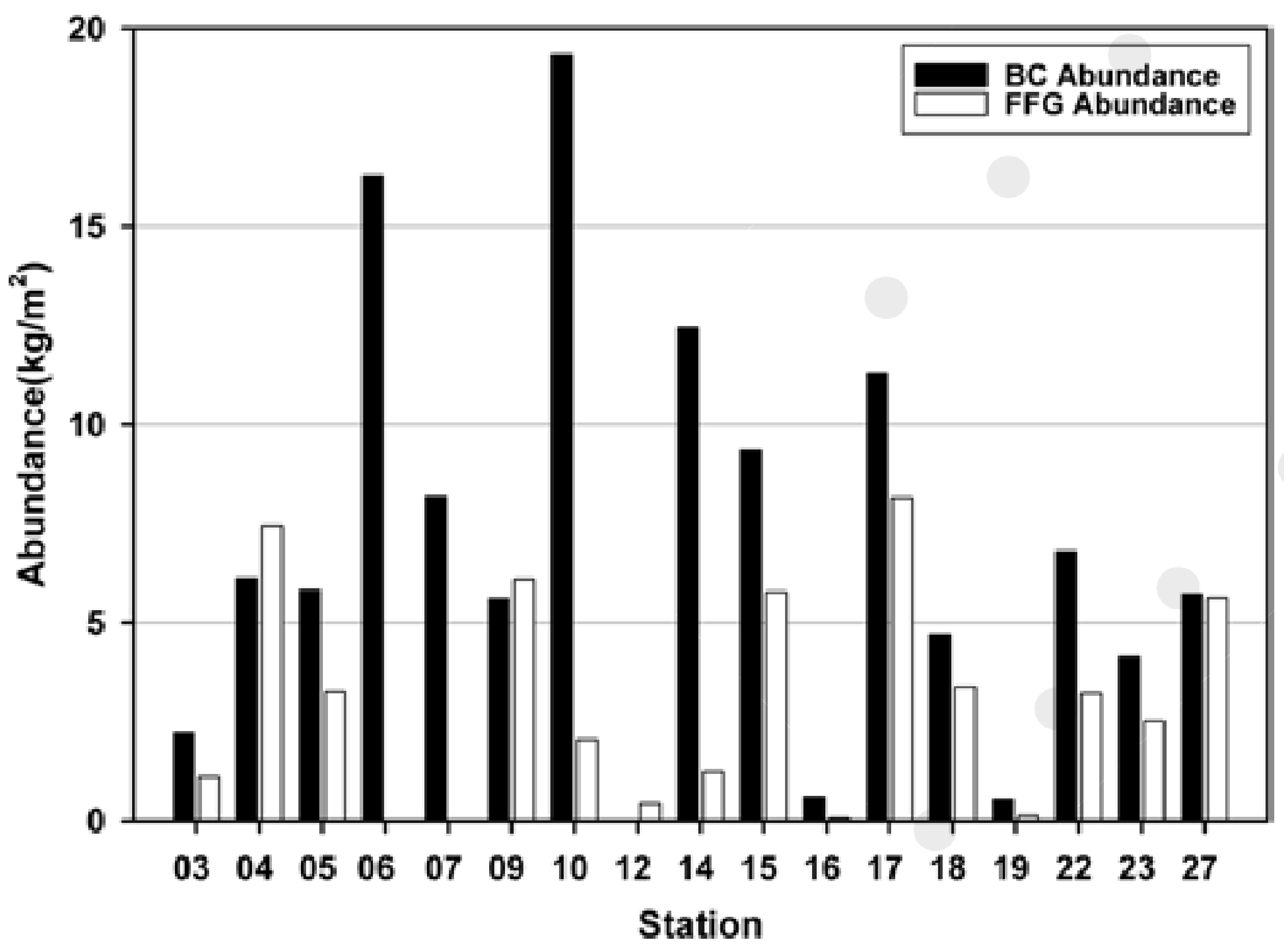
| Historical samples from FFG and BC | Critical for grades and abundance estimates | Critical for grades and abundance estimates | Support for grades and abundance estimates | Not needed |
| Multibeam bathymetry and backscatter | Not available | Used in some areas for model domaining | Needed for model domaining | Needed for model domaining |
| BC physical samples with full QA/QC and chain of custody | Not available | Used in TOML Area F for grades and abundance estimates | Critical for grades and abundance estimates | Critical for grades and abundance estimates |
| Long-axis estimates of nodule abundance | Not available | Not available | Support for estimates in some areas | Critical for estimates |
| Higher-resolution side-scan sonar seafloor mapping | Not available | Not available | Not needed | Support for model domains |
| Criterium | TOML B5338 | TOML B1 | TOML C1 | TOML D1, D2 | TOML F1 | TOML F | Other Areas |
|---|---|---|---|---|---|---|---|
| Level of confidence | measured | indicated | indicated | indicated | indicated | inferred | inferred |
| Block size | 1.75 × 1.75 km | 3.5 × 3.5 km | 3.5 × 3.5 km | 3.5 × 3.5 km | 3.5 × 3.5 km | 7 × 7 km | 7 × 7 km |
| Historic sampling | referred to | included | included | included | included | referred to | generally, < 20 × 20 km |
| Box-core spacing | ~7 × 7 km | ~7 × 7 km | ~15 × 15 km offset | ~7 × 7 km | ~7 × 7 km | ~20 × 20 km offset | not needed |
| Photo-profile (abundance only) | relied at ~3 km × 3.5 km, (verified at ~30 m × 3.5 km) | included at ~3 km × 7 km | relied at ~3 km × 7 km | not used (clay-ooze cover) | not used (operational reasons) | not needed | not needed |
| Variable | Samples | Minimum | Mean | Median | Maximum | Var | CV |
|---|---|---|---|---|---|---|---|
| Abundance (kg/m2) | 527 | 0 | 10.20 | 9.16 | 30.77 | 39.35 | 0.61 |
| Mn (%) | 338 | 6.54 | 28.09 | 28.71 | 33.79 | 10.414 | 0.11 |
| Ni (%) | 338 | 0.33 | 1.26 | 1.31 | 1.55 | 0.03 | 0.14 |
| Cu (%) | 338 | 0.22 | 1.11 | 1.16 | 1.51 | 0.045 | 0.19 |
| Co (%) | 338 | 0.02 | 0.22 | 0.22 | 0.35 | 0.003 | 0.24 |
| Variable | Nugget | Spherical Structure 1 | Spherical Structure 2 | Anisotropy Ratio | ||||
|---|---|---|---|---|---|---|---|---|
| C0 | C1 | Range H1 | C1 | Range H2 | ||||
| 060° (km) | 150° (km) | 060° (km) | 150° (km) | |||||
| Mn | 0.21 | 0.37 | 5 | 10 | 0.42 | 15 | 30 | 0.5 |
| Ni | 0.21 | 0.37 | 5 | 10 | 0.42 | 15 | 30 | 0.5 |
| Cu | 0.21 | 0.37 | 22 | 22 | 0.42 | 70 | 70 | 1.0 |
| Co | 0.21 | 0.37 | 22 | 16 | 0.42 | 70 | 50 | 0.714 |
| Variable | Nugget | Spherical Structure 1 | Spherical Structure 2 | Anisotropy Ratio | ||||
|---|---|---|---|---|---|---|---|---|
| C0 | C1 | Range H1 | C1 | Range H2 | ||||
| 060˚ (km) | 150˚ (km) | 060˚ (km) | 150˚ (km) | |||||
| Abundance | 0.40 | 0.60 | 5 | 5 | – | – | – | 1.0 |
Publisher’s Note: MDPI stays neutral with regard to jurisdictional claims in published maps and institutional affiliations. |
© 2021 by the authors. Licensee MDPI, Basel, Switzerland. This article is an open access article distributed under the terms and conditions of the Creative Commons Attribution (CC BY) license (http://creativecommons.org/licenses/by/4.0/).
Share and Cite
Parianos, J.; Lipton, I.; Nimmo, M. Aspects of Estimation and Reporting of Mineral Resources of Seabed Polymetallic Nodules: A Contemporaneous Case Study. Minerals 2021, 11, 200. https://doi.org/10.3390/min11020200
Parianos J, Lipton I, Nimmo M. Aspects of Estimation and Reporting of Mineral Resources of Seabed Polymetallic Nodules: A Contemporaneous Case Study. Minerals. 2021; 11(2):200. https://doi.org/10.3390/min11020200
Chicago/Turabian StyleParianos, John, Ian Lipton, and Matthew Nimmo. 2021. "Aspects of Estimation and Reporting of Mineral Resources of Seabed Polymetallic Nodules: A Contemporaneous Case Study" Minerals 11, no. 2: 200. https://doi.org/10.3390/min11020200