Article

Possibilities and Limitations of the Use of Seafloor Photographs for Estimating Polymetallic Nodule Resources—Case Study from IOM Area, Pacific Ocean

by
Monika Wasilewska-Błaszczyk
* and
Jacek Mucha
Department of Geology of Mineral Deposits and Mining Geology, Faculty of Geology, Geophysics and Environmental Protection, AGH University of Science and Technology, 30-059 Cracow, Poland
*
Author to whom correspondence should be addressed.
Minerals 2020, 10(12), 1123; https://doi.org/10.3390/min10121123
Submission received: 25 September 2020 / Revised: 9 December 2020 / Accepted: 11 December 2020 / Published: 14 December 2020
(This article belongs to the Special Issue Exploration of Polymetallic Nodules)

Abstract

:
Direct seafloor sampling using, e.g., box corers is insufficient to obtain an acceptable accuracy of nodule resource estimates in small parts of potential deposits. In order to increase the reliability of the estimates, it was rational to use the results of photographic surveys of the seafloor. However, the estimation of nodule abundance based on seafloor photographs is associated with a number of problems and limitations. The main goal of the study was a statistical analysis of the role and interrelationships of selected factors affecting the accuracy of nodule abundance assessment based on seafloor photographs from the H22 exploration block located in the Interoceanmetal Joint Organization (IOM) area in the Pacific. A statistically significant, but only moderately strong, correlation was found between the abundance of nodules and seafloor nodule coverage (quantitative variables), the nodule abundance and genetic type of nodules (ordinal variable estimated visually from photos), and between seafloor coverage with nodules and sediment coverage of nodules (ordinal variable estimated visually from photos). It was suggested that the nodule abundance could be effectively and more accurately predicted using a general linear model that includes both quantitative and ordinal variables.

1. Introduction

The amount of polymetallic nodule resources and the metals they contain is among the more important factors in considering nodule deposits as attractive from the point of view of their future exploitation. Direct sampling of the ocean floor with the use of box corers (or grab sampling, trawl sampling) is insufficient to obtain an acceptable accuracy of resource estimates, especially in small parts of potential deposits, which is important for the development of a detailed exploitation scenario.
In this situation, in order to increase the reliability of the estimates, it was natural and rational to pay attention to the possibility of using indirect methods of determining nodule accumulations, such as the results of hydroacoustic surveys and photographic surveys of the seafloor, carried out systematically and continuously along the course of the research vessel.
The latter method, despite many limitations, significantly supplements the direct sampling and may result in a significant increase in the accuracy of estimation of the nodule abundance. This issue has been the subject of many studies for many years. The nodule parameters (nodule axis lengths, areas of individual nodules, the total area of the seafloor nodule coverage) determined on the basis of subsequent photographs can be treated as soft data [1].
The literature on the subject presents many statistical formulas combining the nodule abundance with the percentage of seafloor nodule coverage [1,2] or nodule parameters determined on the basis of seafloor photographs [3,4,5]. The estimation of seafloor nodule coverage on the seafloor photographs is based on manual or automatic (using computer software) contouring of nodules. Multi-beam data [6] were also used for this purpose.
The estimation of nodule abundance based on seafloor photographs is associated with a number of problems and limitations, including:
  • The quality of photos and the accuracy of determining the seafloor area covered by each photograph;
  • Errors associated with automatic image processing [7,8];
  • The coverage of nodules with sediments [9];
  • The size distribution of nodules [10,11].
The research conducted for the area administered by Interoceanmetal Joint Organization (IOM) in the Pacific (Clarion–Clipperton Zone) showed that the theoretical relative standard errors of the resource estimates based on direct sampling, in blocks with an area of 300 km2, corresponding approximately to the individual areas to be mined in one year, were in the range of 10–27% with a median equal to 13.0% [12]. They were significantly high and resulted mainly from the large distances between adjacent seafloor sampling stations, ranging from 3.3 to 15 km depending on the stage of exploration in the different parts of IOM area. In the case of continental equivalents of oceanic ore deposits, the sampling intervals are many times smaller. The long distances between sampling sites are forced by the costly and time-consuming exploration of a vast area, which in the case of a pioneering investor, such as the IOM, is 75,000 km2.
Combining the box corer data with photographic data resulted in a clear reduction in the theoretical standard errors of estimation from 10–27% to approx. 3–9% with a median of 6% [12]. However, these errors are somewhat underestimated; in the resource estimation method used (ordinary kriging), the authors did not take into account the errors of nodule abundance estimation using the linear regression model that links them to the seafloor nodule coverage determined from photographs.
In the Clarion–Clipperton zone (CCZ), there are three genetic types of nodules (H, HD, and D) [13,14,15]. The individual genetic types of nodules differ in, among others, geometric features, dominant morphotypes, textures, dominant Mn minerals, and the average contents of major metals, which is discussed in detail by Kotliński [14]. Some of the geometric parameters allow an initial visual assessment of the genetic type of nodule based on seafloor photographs. These include range of size, average size, mean diameter, and the fraction distribution. The literature confirms the strong relationship between the individual nodule wet weight and its geometrical features such as nodule long axis [5] or nodule area [16]. The use of this relationship in practice is limited because of the natural coverage of nodules with sediments. The degree of covering the nodules with sediments may be very different. Therefore, the underestimation of the nodule abundance is highly variable. The issue, related to sediment layer obscuring portions of some nodules and completely covering others, was pointed out by Felix [3], Kuhn and Rathke [16], and Sharma [17,18,19]. Owing to the variable burial of nodules under the top sediment layers, Sharma et al. [20] proposed correction factors for empirical formulas. In addition, Jung et al. [9] included the coverage of nodules with sediments in the regression equations.
It is also worth mentioning that in addition to the often successful, indirect nodule sampling methods (using seafloor photography or the results of various hydroacoustic surveys), new techniques for analyzing the data on nodule abundance, such as, for example, geostatistical simulations [21], artificial neural networks [22,23], random forests machine learning [24], and for bottom sediments—multivariate geostatistics [25] are also being proposed.
The main reason of interest in marine mineral deposits such as polymetallic (manganese) nodules, Co-rich ferromanganese crusts, and massive sulfide deposits is increasing demand for critical metals [26,27], i.e., those that have high supply risk and whose shortfall can have a major economic impact [28]. Over the next two decades, a substantial increase in the global consumption of nickel, copper, and cobalt metals that are contained in high concentrations in the mineral resources of the deep sea and are highly important to the economy of the European Union, is expected [29].
These and other metals are essential for the fabrication of high technology, green technology, emerging industries, and military applications (e.g., computer chips, electric vehicles, wind turbines, cellular phones) [26,28,29,30,31]. The decrease in the supply of metals, important for advanced technologies, is the result of the depletion of terrestrial metal deposits and the continuous reduction in their content in ores [26,27,31,32].
Polymetallic marine nodules are an attractive metal source due to the scarcity of high-grade metals in onshore deposits [33]. Nodules contain large variety of metals such as: Cu, Ni, Co, Li, Mo, Te, Ti, Y, Pt, Zn, Zr, Ge, REEs, and Mn [30,31,32,33,34,35,36].
Deep-sea polymetallic nodules are traditionally considered as a vast potential resource for such metals as Cu, Ni, Co, Fe, and Mn, the latter being the most abundant with an average content of around 24% [31,33]. In 2020, the European Commission published a new list of critical raw materials, including metals such as cobalt, HREEs, lithium, and LREEs occurring in significant amounts in nodules [37].
The Clarion–Clipperton Fracture Zone (CCZ) in the tropical NE Pacific is the area of greatest economic interest for nodules [32]. Nodule resources are conservatively estimated to total 21 billion dry tons [30].

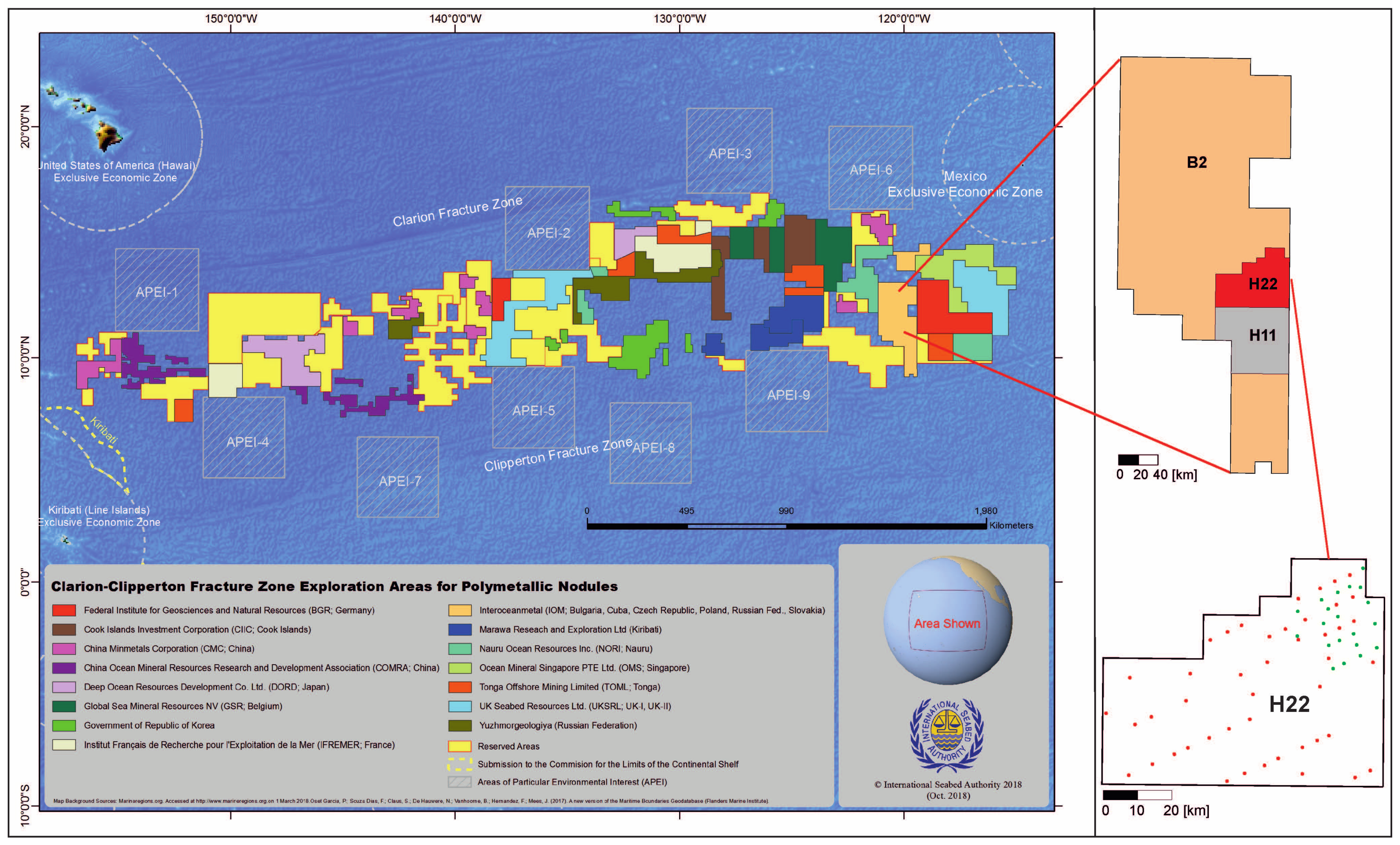
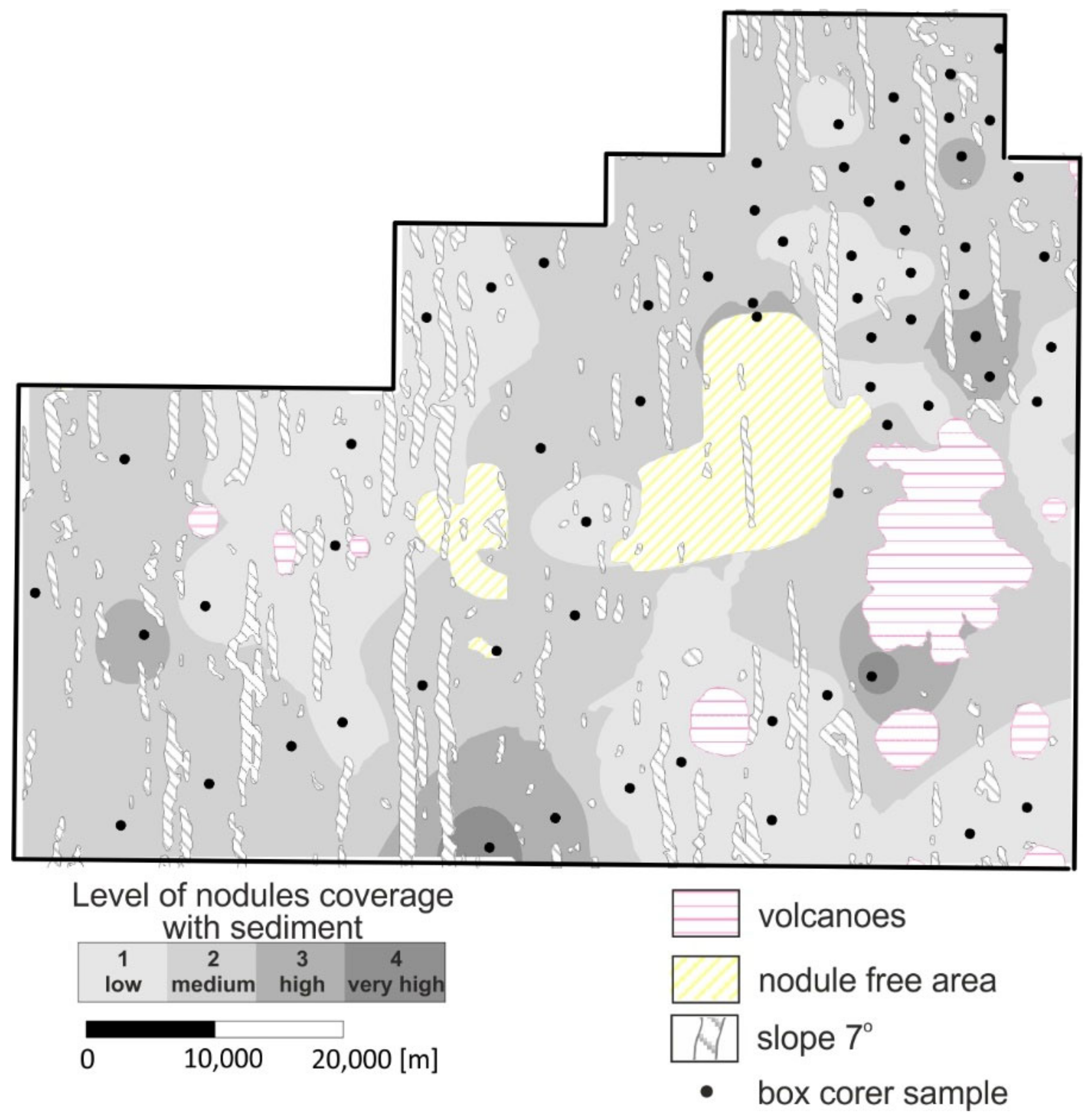
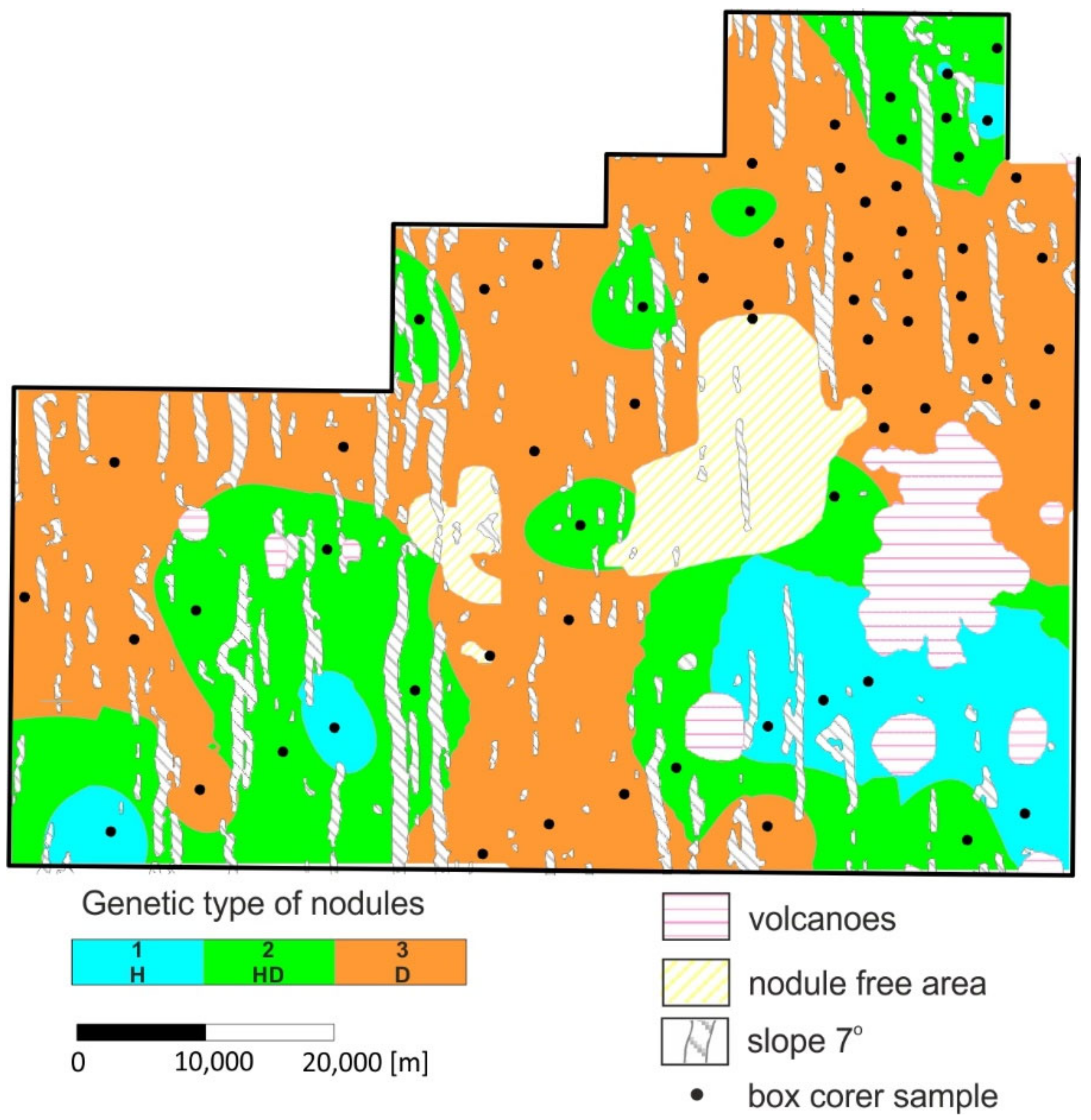
2. Research Objective and Study Area

The main goal of the research was to analyze the role and interrelationships of factors affecting the accuracy of nodule abundance assessment based on seafloor photographs from the H22 exploration block located in IOM area in the Pacific (Figure 1). In particular, the study examined the following factors:
  • The percentage of seafloor nodule coverage at seafloor photography sites;
  • Genetic types of nodules in the context of their fraction distribution;
  • Coverage of nodules with bottom sediments;
  • Nodules fraction distributions.
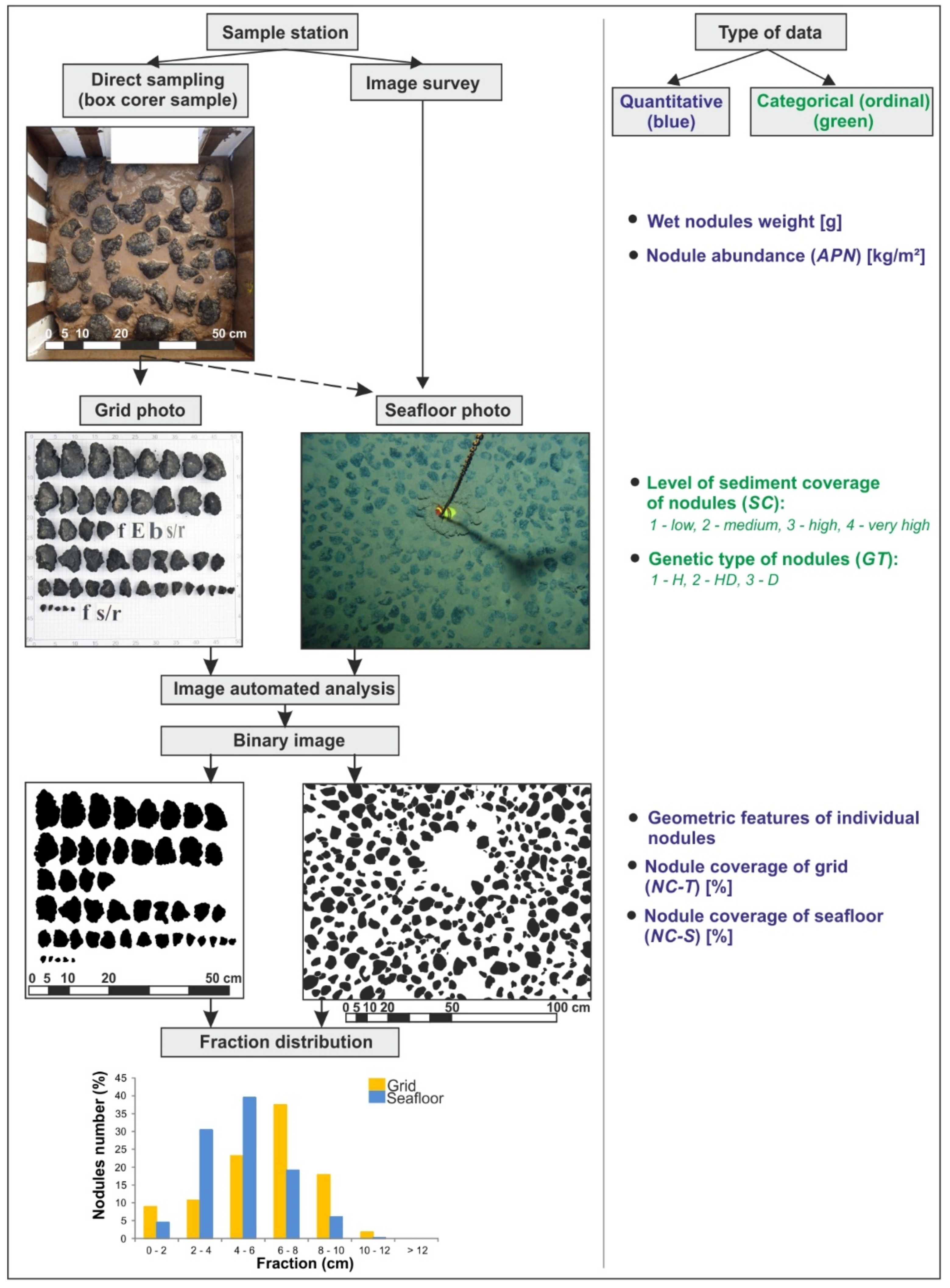
Figure 1. Location of B2 Interoceanmetal Joint Organization (IOM) area and H22 and H11 exploration blocks against the background of Clarion–Clipperton Zone Exploration Areas for Polymetallic Nodules [45]; location of box corer sampling sites and seafloor photographs in H22 exploration block (red—2014 cruise, green—2019 cruise).
Minerals 10 01123 g001
The second goal was to indicate, on the basis of the conducted analysis, the possibility of including significant factors in statistical, advanced regression models in order to increase the accuracy of the prediction of the nodule abundance.
The intergovernmental consortium IOM is a contractor of International Seabed Authority and in accordance with UNCLOS convention has exclusive rights to deep sea exploration, evaluation, and exploitation of polymetallic nodule deposits within a 75,000 km2 area situated in the Clarion−Clipperton Fracture Zone in tropical eastern Pacific region [31,38,39,40]. They cover large seafloor spaces at depths greater than 3500 m. The IOM exploration area is located between 10° and 15° north and consists of two sectors: B1 (with an area of 12,000 km2) and B2 (63,000 km2). The larger B2 sector is more abundant in polymetallic nodules (Figure 1). It is generally believed that the exploitation of ore fields with wet nodule abundance above 10 kg/m2 [31,41] and Ni + Cu + Co content above 2.5% [42,43] or with mean Fe/Mn ratio of 0.3 [44] may be economically viable in the future. The most promising exploration blocks H22 (4200 km2) and H11 (5300 km2), with wet nodule abundance often significantly exceeding 10 (kg/m2) are part of the B2 sector and show a large potential for future exploitation (Figure 1).

3. Materials

The basic material of the research included the results of direct sampling and routine photographic seafloor surveys in the H22 exploration block, performed during two research cruises, which took place in 2014 (48 samples) and 2019 (20 samples) (Figure 1). It was selected for sampling as a block with the highest degree of exploration in the entire IOM area. The high abundance of nodules is the reason why the exploitation of nodule deposits is expected. Other significant factors were uniform methods of sampling and photographic surveying of the seafloor during the cruises in 2014 and 2019, emphasizing the homogeneity of the obtained data sets from the point of view of their reliability and measurement accuracy.
Direct sampling used a box corer [46] with dimensions of 0.5 m × 0.5 m × 0.5 m (Figure 2); therefore, at each sampling station, the area of the sampled seafloor was 0.25 m2. The quantitative measure of the seafloor nodule coverage was the nodule abundance (APN (kg/m2)) [15], defined as the ratio of the mass of the extracted wet nodules to the area of the horizontal cross section of the box corer. An image of the seafloor was taken just before sampling with the box corer (Figure 2). The seafloor area covered by the photograph was variable and ranged from 1.23 to 1.80 m2, with an average value of 1.58 m2. The exact location of the sampling site in relation to the seafloor area covered by the photograph was not known, but it can be assumed with a high probability that the sample was collected within its limits. In the case of 6 out of 68 sampling sites, no seafloor photo was taken before the box corer sample was collected; therefore, seafloor photographs obtained from photo-profiling (the device Neptun C-M1, Russia [47]), covering an area of approximately 5 m2 located at a distance of 5–50 m from the direct box corer sampling site, were used.
The abundance of nodules (APN (kg/m2)) was determined for all sampling stations based on box corer samples; the percentage of grid coverage with nodules after their removal from the box corer (NC-T) and the percentage of seafloor nodule coverage determined based on seafloor photographs (NC-S) were assessed. The dominant genetic type of nodules was determined based on seafloor photographs and the level of the nodule coverage with sediments was assessed visually; both parameters were coded as categorical or, more precisely, ordinal variables (Figure 2). Contouring of nodules in seafloor photographs for the purpose of determining the coverage (NC-S) was conducted automatically (manual contouring was conducted for control purposes). The granulometric distributions of the nodules (fraction distributions) were determined for the collected samples and seafloor nodule photographs.
Because of the approximately six times smaller horizontal surface of the box corer and of the seafloor area covered by the photographs, the nodule abundances measured directly and estimated indirectly from the photographs can be clearly differentiated. This difference may be due to a number of factors. Natural factors include the local variability in the seafloor nodule coverage within the sampled bottom areas and the local variability in the nodule coverage with sediments and their partially burial in the sediment. The method of contouring nodules in the photograph (manual or automatic) is a technical factor whose impact on the observed differences in abundances is relatively small. According to Sharma et al. [7], the good positive correlation (with a determination coefficient > 0.98) recorded between visual and computed estimates confirms that both estimation methods are highly reliable. However, the digitally computed estimates were approximately 10% higher than the visual estimates of the same images. Schoening et al. presented a computational image analysis approach using artificial neural network to quantify nodule coverage with a correlation of 0.95 between the expert’s estimate and the automated approach [48]. The method of automatic nodule contouring described by Kuhn and Rathke [16] gives good results for nodules of various sizes; however, the accuracy of this method is limited when the nodules are covered with sediments.
The correlation relationship between the seafloor nodule coverage determined manually and automatically (using computer software) was examined for the part of the data set (from 2014). A very strong linear correlation between the seafloor nodule coverage determined manually (NC-S(M)) and automatically (NC-S(A)), with the correlation coefficient 0.966 (R2 = 93.3%), was found. The least squares linear regression equation is:
NC-S(M) [%] = −6.86 + 1.06∙NC-S(A) [%]
The Student’s t test showed (at the significance level of 0.05) that in the case of the slope, there was no reason to reject the hypothesis that it is 1 in the general population (p-value = 0.188 for the two-tailed test), while in the case of intercept, the hypothesis that it is equal to 0 should be rejected (p-value = 0.000 for two-tailed test). The obtained results indicated the fixed bias [49] in the manual assessment (NC-S(M)) based on the automatic assessment (NC-S(A)).
Generally, the manual method gave more conservative (more careful) estimates of the seafloor nodule coverage, on average about 7% lower than the automatic method. This is in line with the observations made by Sharma et al. [7] who estimated this difference at approximately 10%.
It should be noted, however, that reordering the variables may lead to slightly different conclusions. The relationship model is expressed as follows:
NC-S(A) [%] = 8.60 + 0.88∙NC-S(M) [%]
In the case of perfect agreement between both measurements in the equation of dependence, the intercept is equal to zero and the slope is equal to 1.
In this case, the Student’s t test showed (at the significance level of 0.05) that the hypothesis that the slope value in the general population is 1 should be rejected (p-value = 0.002 for the two-tailed test), and the hypothesis that the intercept is 0 should be also rejected (p- value = 0.002 for a two-tailed test). The obtained results indicate both the proportional and fixed bias [39] in the automatic assessment (NC-S(A)) based on the manual assessment (NC-S(M)).
Based on the above-mentioned results, it can be stated that providing the value of the correlation coefficient (which is a common practice) is not enough when determining the relationship between the variables. The analysis of the parameters of the model aimed at determining the occurrence of potential biases expressed by statistically significant deviations of the intercept from 0 (which is demonstrated by the fixed bias) and slope from 1 (which is demonstrated by the proportional bias) is required.

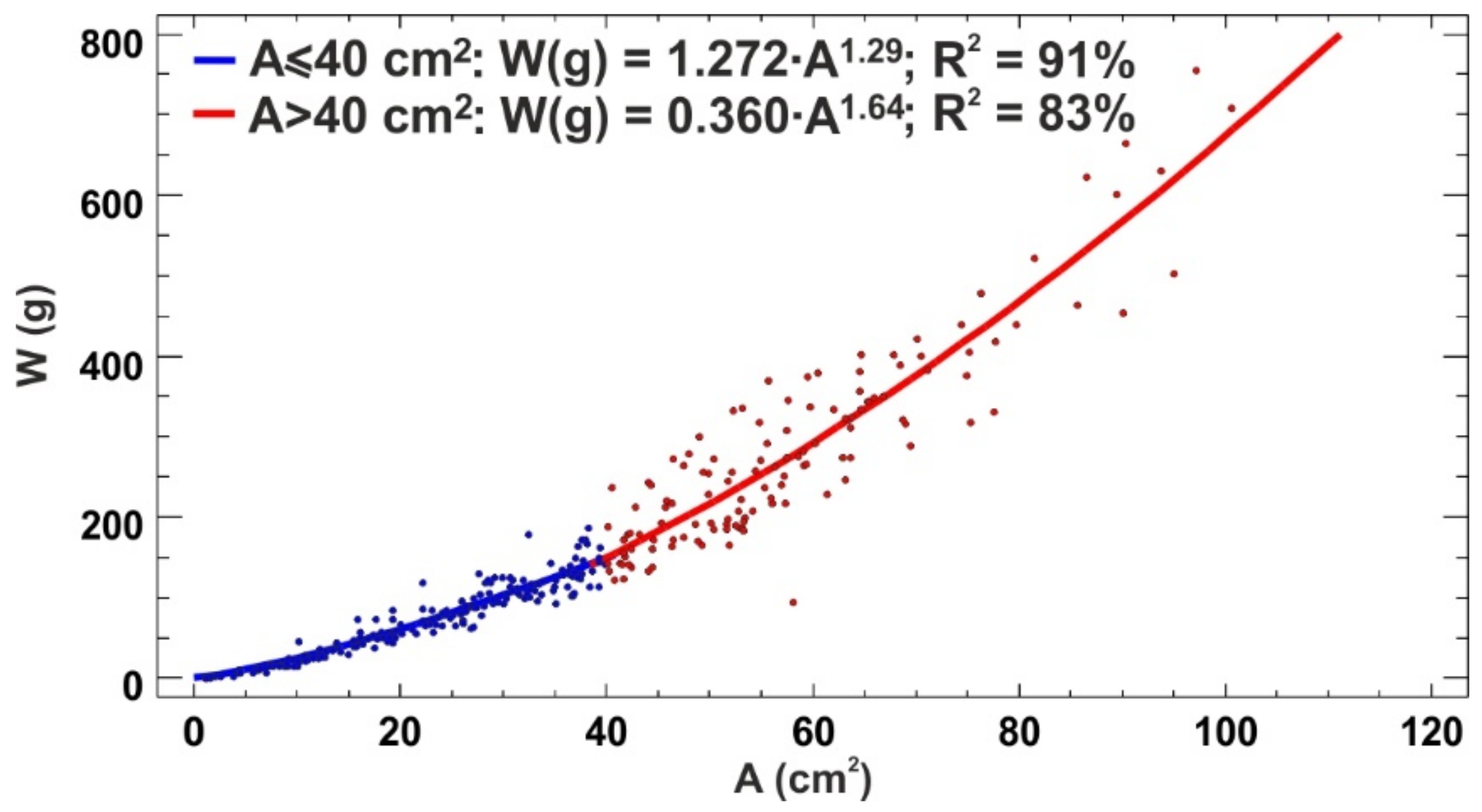
4. Analysis of the Factors Affecting the Effectiveness of the Use of Photography to Assess the Nodule Abundance

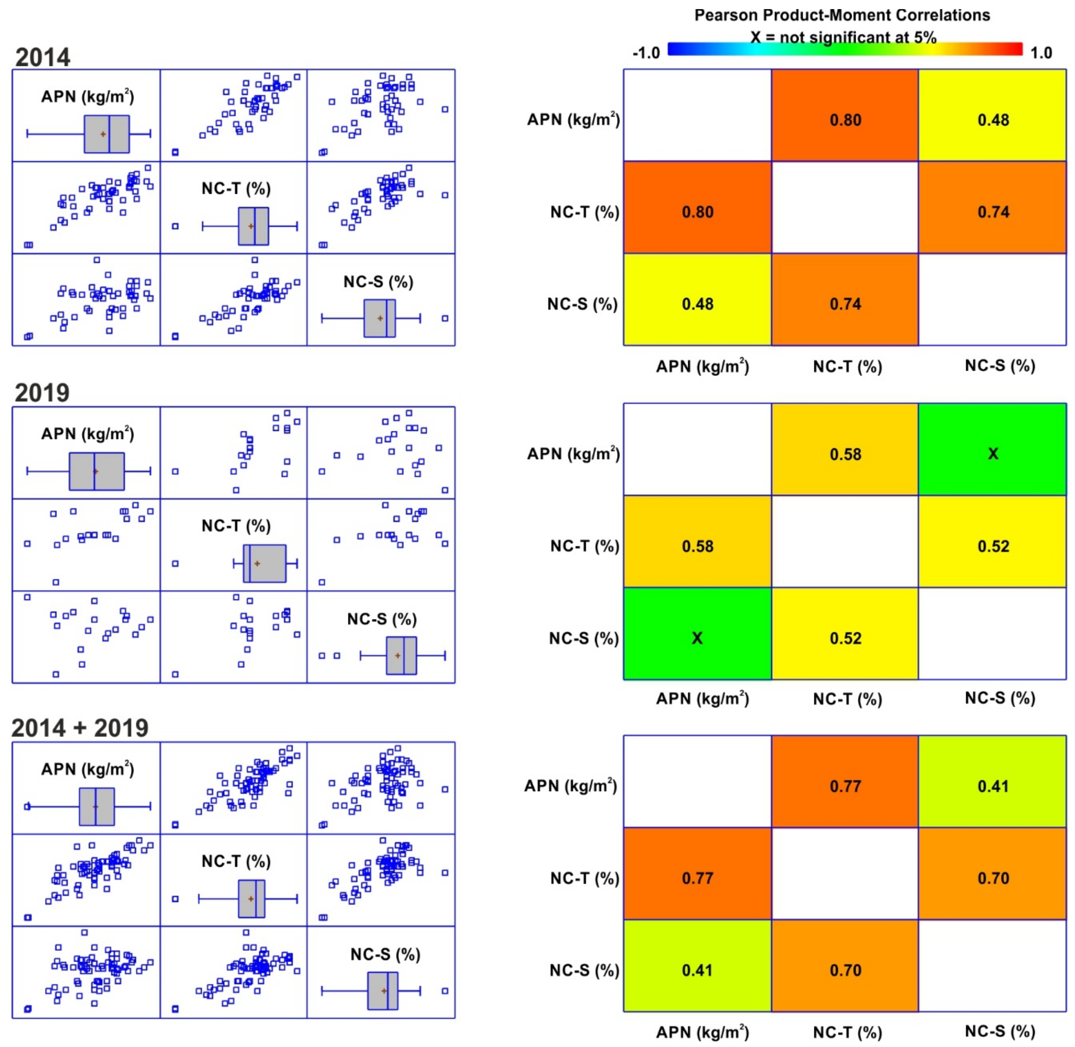
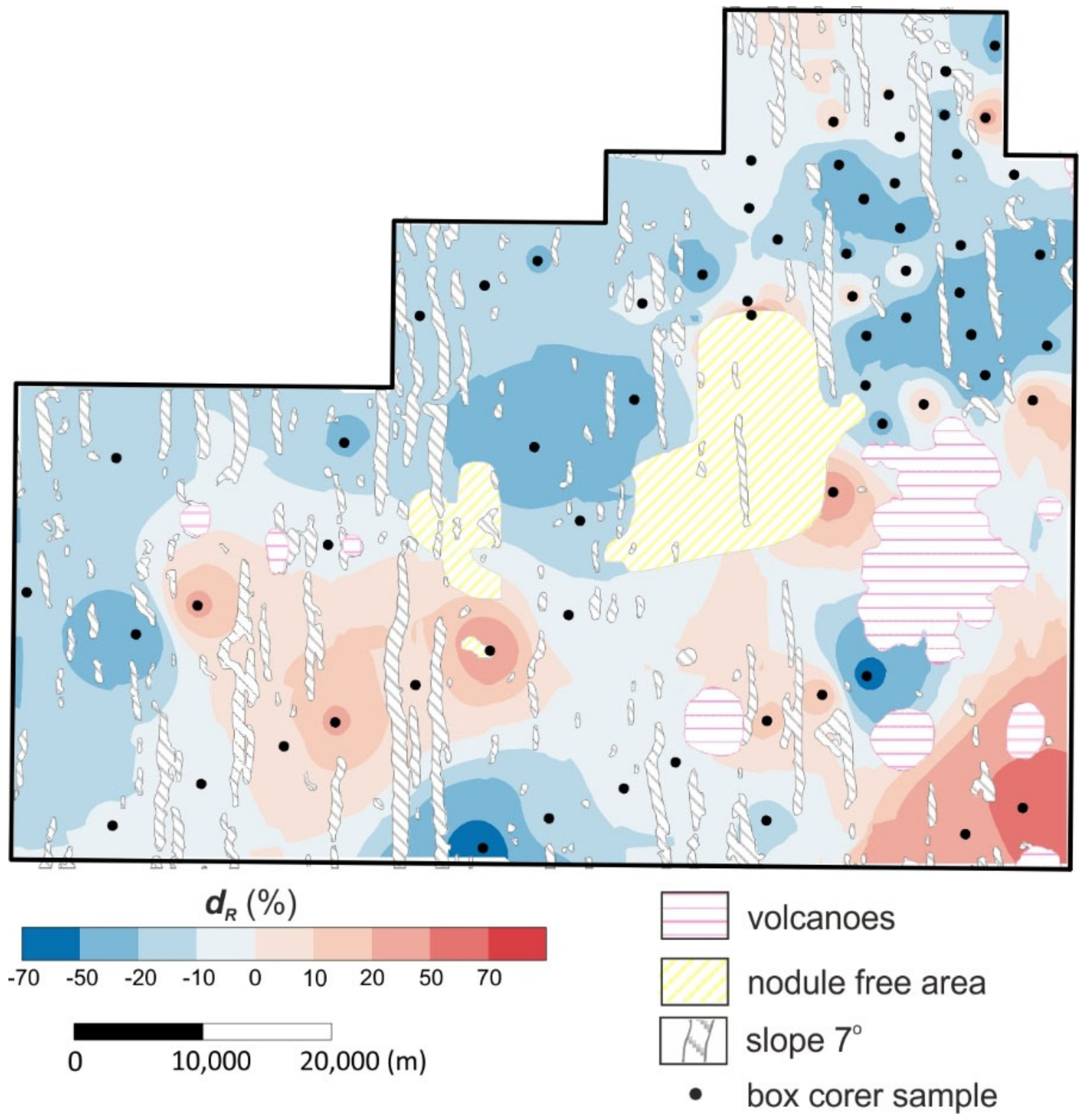
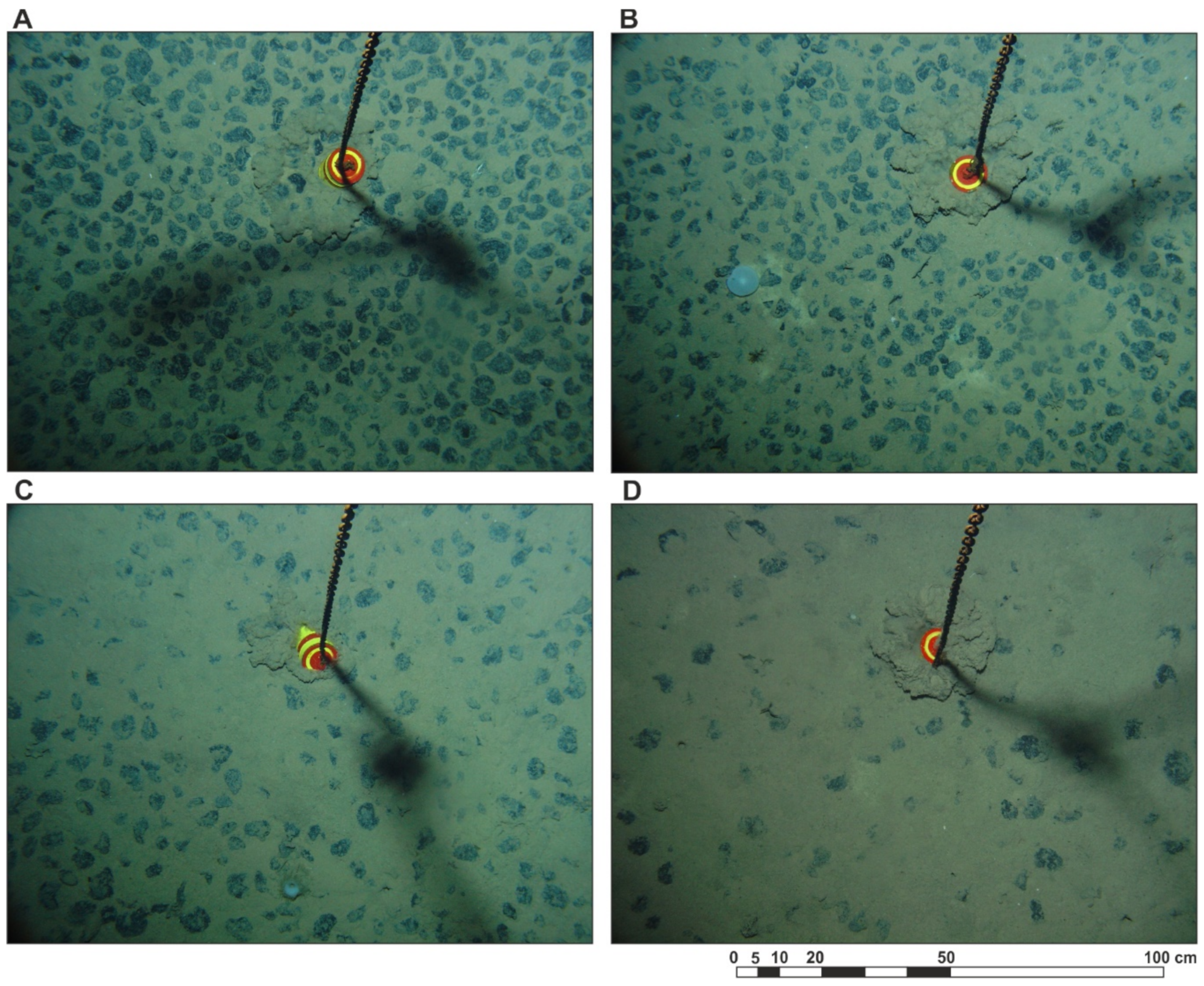
4.1. Statistics of the Nodule Coverage of the Seafloor and the Grid and the Nodule Abundance in Block H22

The values of the basic statistical parameters of nodule abundance (APN), seafloor coverage with nodules in the photograph (NC-S), and nodule coverage of the grid (NC-T) are summarized in Table 1, while the strength of the linear correlation between the parameters is shown in Figure 3.
The ranges of nodule coverage of the seafloor and the grid were very similar (from 5.0% to 72.0%) (Table 1). However, in line with previous experience, the average seafloor nodule coverage (NC-S) was lower than the average grid nodule coverage (NC-T) and for the considered data set it was approximately 6%, although for other parts of the IOM area, it sometimes exceeded 10%. The empirical distributions of all three parameters showed negative asymmetry and their variability with the coefficient of variation (CV) in the range of 29–35% can be described as average or moderate. It was much lower than for the entire B2 sector, where it was about 60% [50] and which may be associated with a slight upward trend in the nodule abundance in the N-S direction.
For the combined subsets of dataset from 2014 and 2019, the nodule abundance (APN) showed a strong linear correlation with the nodule coverage in the grid photo (with the correlation coefficient r = 0.77) and weak with the nodule seafloor coverage determined automatically from the photos (r = 0.41). It should be noted, however, that the strength of the correlation varied depending on the considered data subset. For example, in the H22 exploration block, for data from all samples collected before the last cruise in 2019, the linear correlation coefficient for the pair (APN)–(NC-S) was much higher and amounted to 0.64 [12]. According to Kuhn and Rathke [16] in the German license area of CCZ, the correlation (APN)–(NC-S) does not occur at all, which the authors associate with the occurrence of nodules of large size.
The nodules occurring on the seafloor are usually visible in the photographs. The nodules are partly or fully embedded in clays and siliceous oozes of the geochemically active layer (2–12 cm thick), in which they were formed [14]. This layer is known as the sediment–water interface boundary (SWIB layer) [51]. The degree of embedding depends on the thickness of the SWIB layer and directly affects the accuracy of nodule abundance estimation from seafloor photographs [14]. Nodules are considered to be covered with sediments if they are at a depth of up to 10 cm, while the buried nodules lie beneath the active sediment–water boundary layer [52]. The buried nodules are not taken into account when calculating the abundance of surface nodules and, therefore, they are not the subject of this paper. From the point of view of future exploitation, both the surface nodules and nodules covered with sediment (up to 10 cm) are considered to be recoverable.
The measure of the degree of coverage of nodules with sediments used in the literature is the ratio of the area of the grid covered by the nodules to the seafloor area covered with nodules [14], which usually ranges from 1 to over 10. Sometimes, however, it takes a value less than 1, which proves that the seafloor nodule coverage is greater than that found for the box core sample. This measure for the H22 exploration block ranges from 0.6 to 2.6. Values less than 1 can be explained by the local variability of the seafloor nodule coverage.
The lack of information about the location of the box corer in the seafloor photograph requires the comparison of nodule coverage on two significantly different surfaces: 0.25 m2 (horizontal box corer area) and approximately 1.6 m2 (photographed seafloor area). However, because of local changes in the coverage of nodules with sediments and the nodule coverage of the seafloor, this measure has serious shortcomings and can be treated as an approximate one.
This study used a different measure of nodule coverage based on calculating the relative difference in the percentage of seafloor nodule coverage (NC-S) and grid (NC-T) at each sampling station from the following formula:
d R = NC - S     NC - T NC - T × 100 %
This measure is also imperfect and approximate but does not cause numerical problems when no nodules are found in the grid (NC-T = 0%) but the nodule coverage is visible in the seafloor photographs. Negative values indicate a greater influence of local variability of nodule abundance, while positive values indicate a greater influence of coverage of nodules with sediments. The measures of coverage of nodules with sediments expressed in this way in the H22 exploration block are presented in the form of contour maps in Figure 4. The relative differences ranged from −62% to 68%. They were negative, i.e., NC-S was smaller than NC-T, in approximately 60% of the sampling stations; in other stations, the situation was the opposite. The relative differences (dR) were significant, i.e., less than −20% or greater than 20%, in more than 40% of the sampling stations in the H22 exploration block (Figure 4).
For the assessment of the nodule coverage with sediments visible in the seafloor photographs, a visual assessment performed by a geologist experienced in the photographic evaluations seems more appropriate and effective.
In the research area, the seafloor photographs showed different degrees of coverage of nodules with sediments (examples are shown in Figure 5). The local increase in coverage of nodules with sediments was often visible only in a part of the seafloor photograph. The increased coverage of nodules with sediments usually affects from a few to even 50% of the area of the photographed seafloor. The experience gained during the manual contouring of nodules on 48 photographs of the seafloor made it possible to subjectively distinguish 4 degrees of their coverage with bottom sediment, which were assigned numerical identifiers from 1 to 4 in accordance with the increasing level of coverage: low coverage (1), medium coverage (2), high coverage (3), and very high coverage (4). The assumed degrees of coverage are visualized in Figure 5 using 4 photographs illustrating the increase in the seafloor sediment coverage. Because of their ordered character, numerical identifiers were treated in the further analysis as ordinal qualitative variables.
The varying degree of coverage of nodules with sediments presented in Figure 5 is clearly reflected in the distributions of the number of nodules for individual fractions, determined on the basis of the grid photograph and seafloor photograph (Figure 6). The distributions of the number of nodules for both data types (photographs) are very similar at low or moderate seafloor coverage with sediments (Figure 6A,B). In this case, the slight differences in the distributions can be explained mainly by the variability of the number of nodules in different parts of the photographed section of the seafloor and variable measurement areas on grid and seafloor photographs. With a high and very high coverage with sediments, the distributions show significant differences expressed in the dominance of smaller fractions (<6 cm) for seafloor photograph and the dominance of large fractions (>8 cm) for grid photograph (Figure 6C,D). This premise justifies the use of at least an approximate visual assessment of the degree of seafloor coverage on the basis of its photographs, which can then be taken into account in regression models linking the nodule abundance (APN) with the seafloor nodule coverage (NC-S).
Based on the subjectively assumed degrees of coverage of nodules with sediments, a map for the H22 exploration block was constructed (Figure 7). It is suggested that the arrangement of the assumed degrees of nodule coverage with sediments is not purely random, although no clear regularities or trends of occurrence within the H22 exploration block were observed. In addition, the visually determined nodule coverage with sediments does not correlate with the distribution of relative differences of percentage nodule coverage of the seafloor and the grid (dR) (Figure 4). A lower or higher degree of coverage of nodules with sediments leads to an underestimation of the size and area of the nodules at the sampling stations, and consequently to systematic errors (underestimation) of the weight assessment of individual nodules based on regression models and, after summing up the weights, the abundance of nodules.
Under laboratory conditions, the regression relationships linking the longer axis or the surface area of the nodule with its weight are strong for nodules cleared of sediments. This is illustrated in the example shown in Figure 8 for a nonlinear (segmented) regression between the nodule surface area and weight. The coefficients of determination were very high and amounted to 0.83 for the fraction with an area of ≤40 cm2 and 0.91 for the fraction with an area >40 cm2, which means that the regression model explains, respectively, 83% and 91% of the variability of the nodule weights. Such a strong relationship allows the determination of weight and, consequently, the nodule abundance with high accuracy. In the case of measurements of surface areas of nodule occurrence in the seafloor photographs, the regression model gave satisfactory results only in those parts of the seafloor in which the nodules were not covered with sediments, which is very rarely observed. This leads to the conclusion that regression models should take into account the degree of coverage of nodules with sediments defined visually and expressed by ordinal variables.

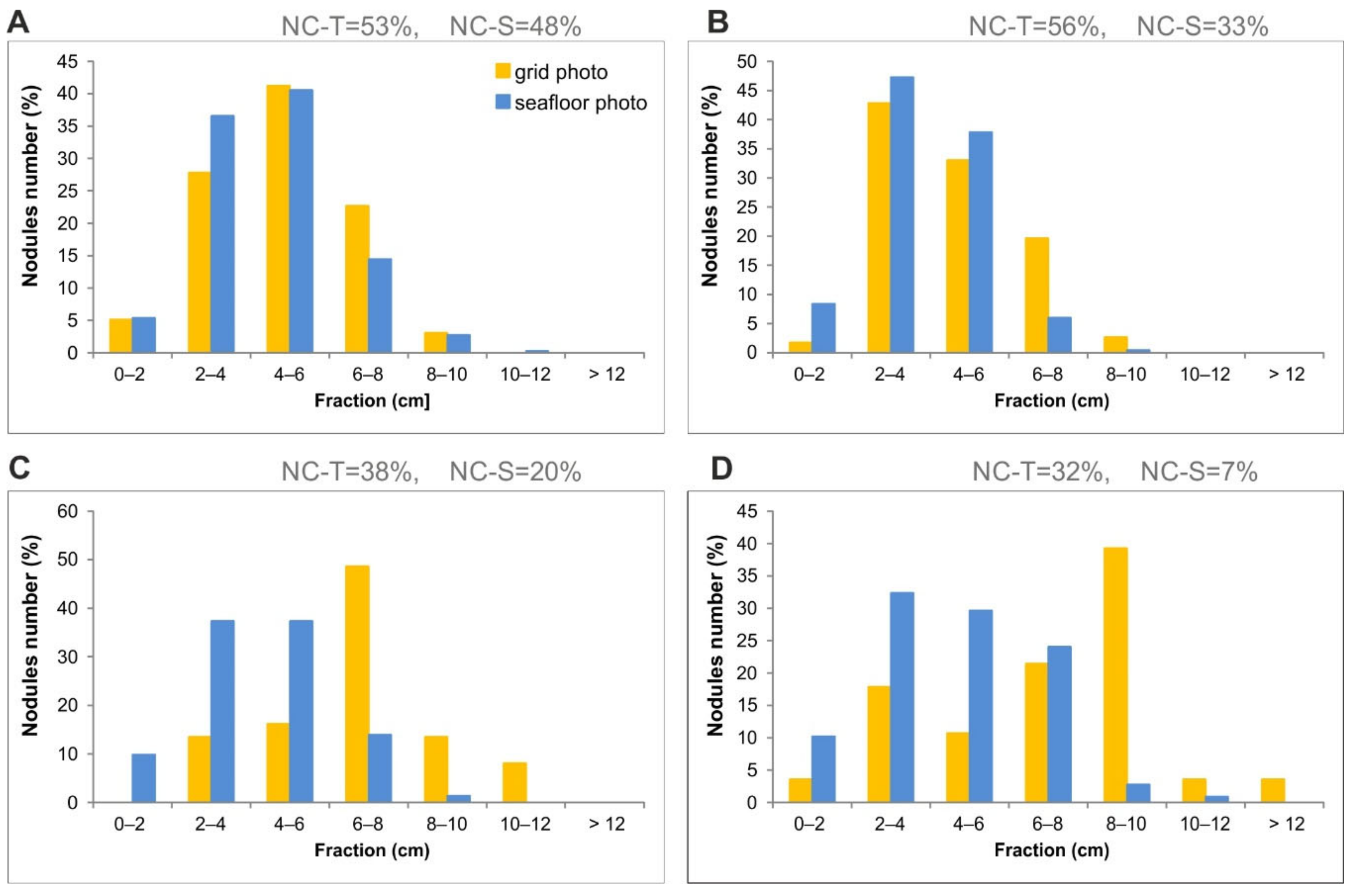
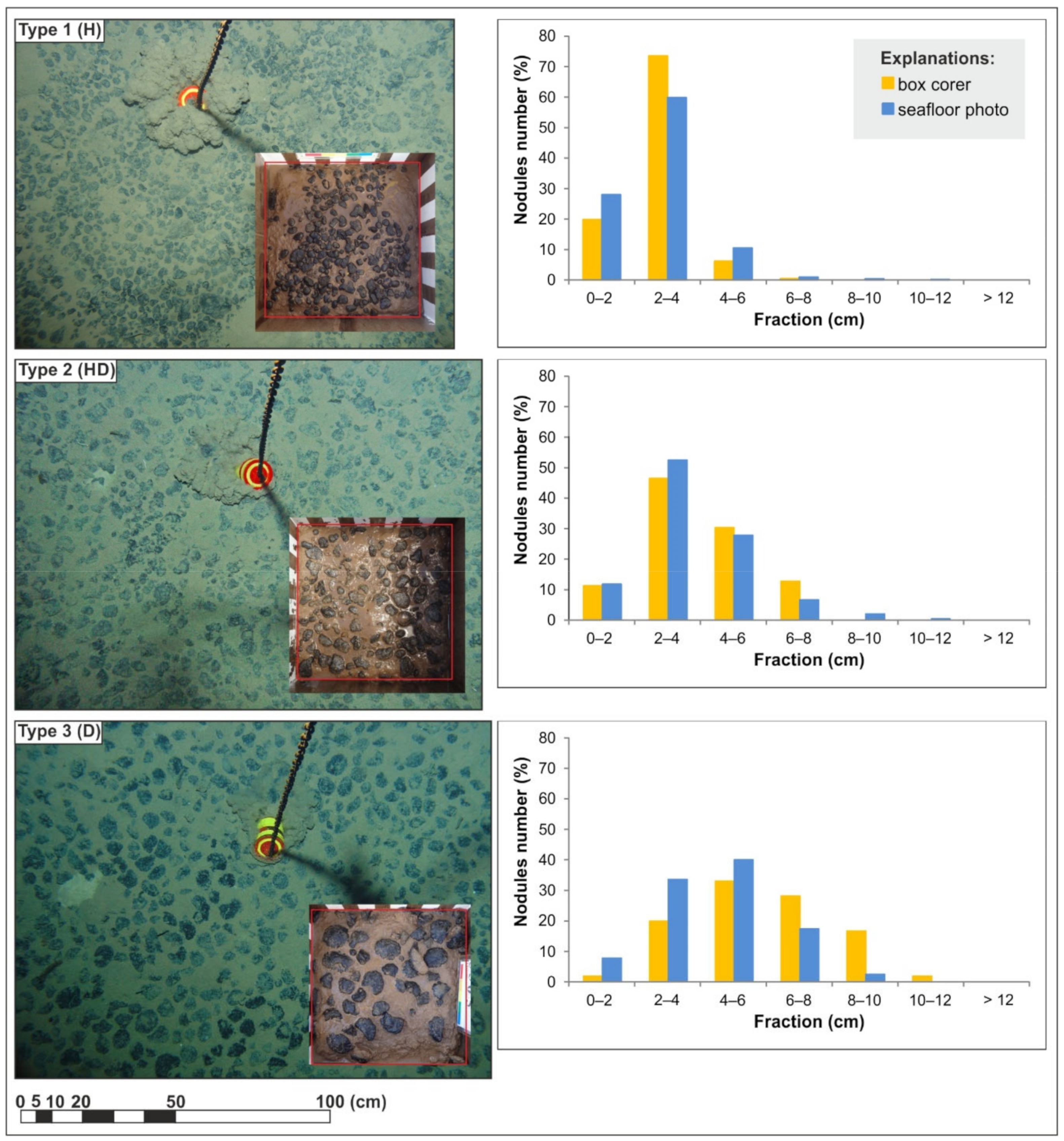
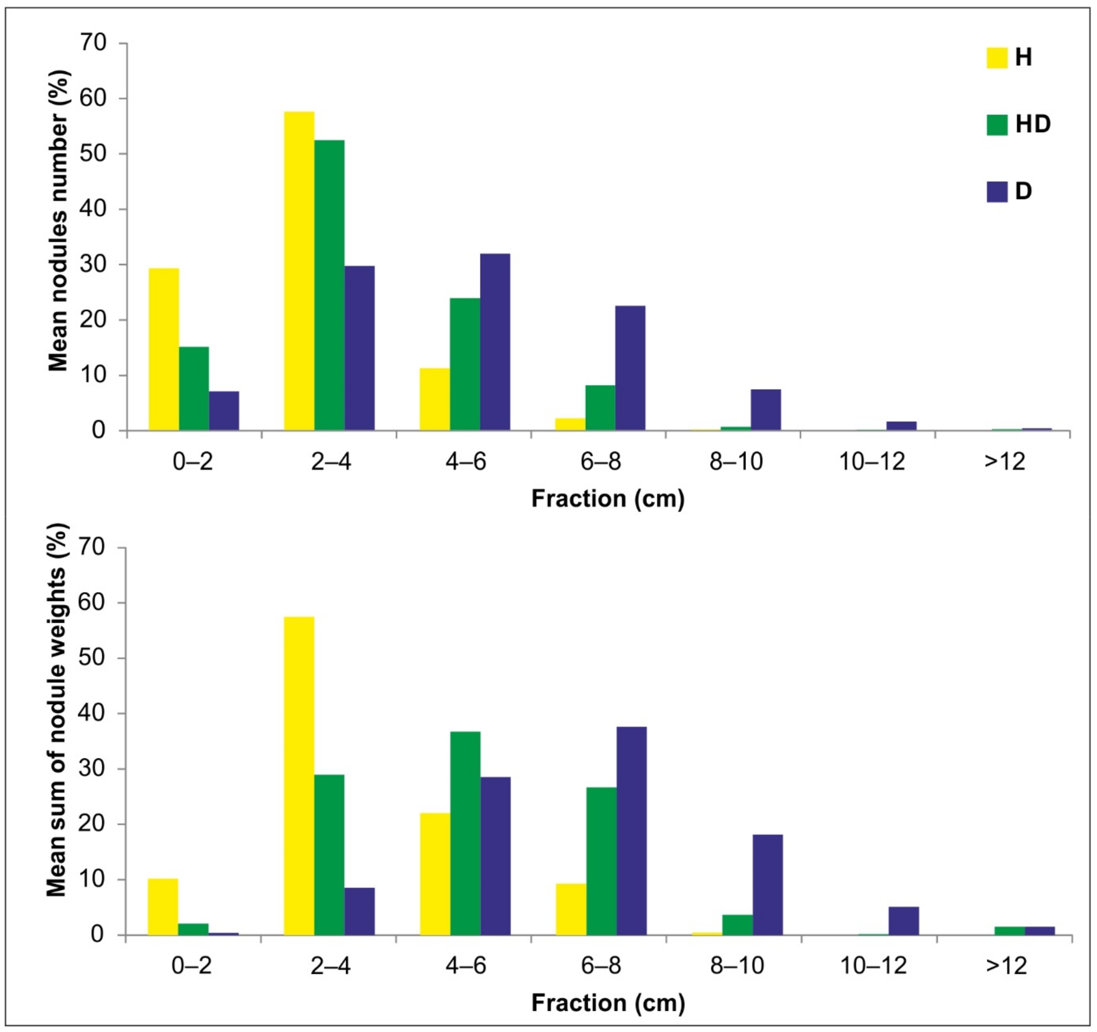
4.2. Genotypes of Nodules and Fraction Distribution

Nodules occurring in the CCZ are most commonly classified into three genetic types [14,15] (Figure 9):
  • Type 1: H (hydrogenetic)—small nodules up to 3 cm [14] or up to 4 cm [15] in diameter, most frequently spheroidal and with smooth surfaces;
  • Type 2: HD (hydrogenetic-diagenetic)—nodules intermediate in size (by convention, from 3 to 6 cm in diameter) with smooth upper and rough lower surface, predominantly ellipsoidal, flattened, and plate-shaped;
  • Type 3: D (diagenetic)—large nodules, 6–12 cm in diameter, predominantly discoidal and ellipsoidal in shape and with rough surfaces.
Figure 9. Seafloor and box corer photographs for three genetic types of nodules (left); fraction distributions of nodules defined on the basis of the box corer and seafloor photographs (right).
Minerals 10 01123 g009
Within the genetic type D, the D1 subtype is distinguished, which differs from type D by a different relation of Ni and Cu contents.
Above, only the morphological features (appearance, size, and the character of outer surface) of the nodules are presented, since only these can be determined from the seafloor photographs. The distinguished genetic types also differ in other features that can be determined under laboratory conditions, such as, e.g., chemical composition.
Figure 9 shows examples of seafloor and box corer photographs with three genetic types of nodules from sample stations from the H22 exploration block. The seafloor photographs are characterized by a relatively small and similar coverage of nodules with sediments. This allowed us to perform a preliminary comparison between the distribution of nodule fractions determined on the basis of box corer and seafloor photographs. Visually, in the case of all three types of nodules, the fraction distributions for these two are quite similar despite the different size of the sampled seafloor area (directly and indirectly). Therefore, it is possible to assume a relatively small local variability (for the scale of observation corresponding to the photographed seafloor area at an individual sampling station) of the seafloor nodule coverage for the three genetic types, and, consequently, for the nodule abundance.
The numbers and weights of nodules averaged for all sampling stations for individual fractions, determined on the basis of seafloor photographs, are shown in Figure 10. They show a clear difference in fraction distributions between the distinguished genetic types of nodules with different class ranges in which there is a dominant (modal value) of weights: 2–4 cm for hydrogenetic, 4–6 cm for hydrogenetic-diagenetic, and 6–8 cm for diagenetic.
Based on the scaled seafloor photographs, it is possible to determine the dominant fractions of nodules, and thus, with high probability, the genetic type of nodules (Figure 9). The factor limiting this action may be a high degree of nodule coverage with sediments. An increased (high) coverage of with sediments often concerns only a part of the photograph. In such a situation, it is possible to determine the dominant nodule type only on the basis of a fragment of the photograph, where the coverage is relatively small. Approximate (initial) information about the size of nodules (predominantly small nodules or large nodules) can be obtained using the acoustic backscatter map [41].
For indicative purposes, the spatial distribution of genetic types of nodules in the H22 exploration block is presented in Figure 11. Generally, the grouping of sampling sites with the same genetic type of nodules, especially diagenetic, is noticeable. This indicates a non-random distribution of genotypes in the analyzed area and the presence of certain regularities in their spatial distribution.
The comparison of the maps presented in Figure 4, Figure 7 and Figure 11 does not allow us to clearly decide whether there is a relationship between genetic types of nodules and their coverage by sediments. It can be provisionally concluded that relatively high nodule coverage with sediments (usually medium or high, and less commonly low) was observed for the genetic type D (diagenetic). However, low nodule coverage with sediments usually was observed in the case of H and HD-type nodules.

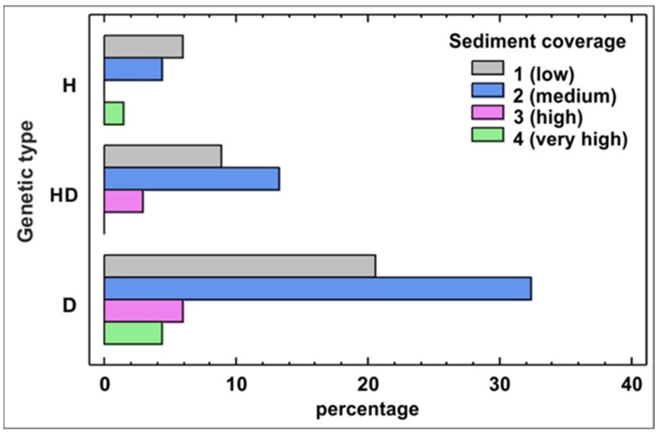
4.3. Homogeneity and Correlation of the Studied Variables

The analysis of correlation was preceded by the examination of the homogeneity of the distinguished genetic types due to three continuous variables characterizing them: nodule abundance (APN) determined on the basis of box corer samples and (1) nodule coverage of the seafloor (NC-S) and (2) nodule coverage of the grid (NC-T), both determined on the basis of photographs. The Games-Howell test, belonging to the family of multiple comparison tests, was used for this purpose [53,54]. Contrary to other tests of this type, its advantage is the possibility of comparing sets with unequal sample sizes or variances.
In the case of APN, it was found that all the analyzed genetic types were heterogeneous and characterized by statistically significant differences of the mean values of this parameter (Table 2). Similar results were obtained for all data from the entire B2 sector (IOM area) (Figure 1) [55].
Surprisingly, the other two variables (NC-S and NC-T) did not show statistically significant differences of means and formed homogeneous sets regardless of the genetic type of nodules. This result suggests that the relationship between APN and NC-S, which should theoretically occur and manifest itself in a similar arrangement of homogeneous groups, is disturbed by the nodule coverage with sediments and masking some parts of nodules. This is confirmed by the results of the correlation analysis presented in Table 3.
Two types of variables were used in the correlation analysis:
  • • Continuous: nodule abundance (APN) and percentage coverage of the seafloor with nodules (NC-S);
  • • Categorical (ordinal): genotype of nodules (GT) (hydrogenetic—1, hydrogenetic-diagenetic—2, diagenetic—3) and the degree of nodule coverage (SC) with sediments (low—1, medium—2, high—3, very high—4).
The strength of the correlation for pairs of variables (continuous–ordinal and ordinal–ordinal) was determined using two measures provided for such variables: Spearman’s rank correlation coefficient and Kendall’s Tau-b correlation coefficient (Table 3) [54]. Similar to the Pearson’s linear correlation coefficient, both measures were in the range [−1, 1], where values close to zero mean no correlation, while an increase in the absolute values of the coefficients to 1 means an increase in the strength of correlation. The statistical significance of the correlation was verified using the p-value for a significance level of 0.05 (p-value ≤ 0.05 means a statistically significant relationship, while p-value > 0.05 indicates no grounds for rejecting the hypothesis of correlation independence of variables). In the case of the correlation of continuous variables (APN-NCS), the values of the Pearson’s linear correlation coefficient were used (Table 3) due to the linear nature of the relationship (Figure 3) and empirical distributions of these variables not drastically different from the normal distribution (Table 1).
The results of testing the statistical significance of correlation were consistent for both measures of dependence represented by Spearman’s and Kendall’s Tau-b correlation coefficients (Table 3). The strongest and statistically significant correlations (for the significance level of 0.05) were observed for the pairs: APN–GT with Spearman’s and Kendall’s correlation coefficients (0.62 and 0.51, respectively), NC-S–SC (−0.69 and −0.57), and APN–NC-S with Pearson’s correlation coefficient of 0.41, while a much weaker correlation was observed for the NC-S–GT pair (−0.26 and −0.21, respectively). However, there are no grounds to reject the hypothesis that there is no correlation relationship between the APN-SC and GT-SC pairs.
This is confirmed by the visual evaluation of the bar chart presented in Figure 12. It can be stated that low and medium coverage with sediments prevailed significantly for all genetic types of nodules. High or very high coverage occurred, however, in all 3 genetic types of nodules, but in similar percentage share from 12% to 16%. Therefore, it can be concluded that the degree of sediment coverage is similar for 3 genetic types of nodules. This is in line with the results of a study on the German license area by Kuhn and Rathke [16], who concluded that sediment coverage did not depend on the size of the nodules.

5. Discussion and Conclusions

The assessment of the abundance and resources of polymetallic nodules in the Pacific based on the results of box corer sampling is subject to significant errors due to the long distances, up to several kilometers between sampling stations. The risk of a meaningful estimation error increases as smaller and smaller parts of the deposit, e.g., intended for exploitation over short periods, e.g., a year or a quarter, are considered. In this situation, it is rational to use a large set of seafloor photographs, taken routinely along the course of the research vessel performing, among others, direct bottom sampling, for the estimation process. The determination of the percentage of seafloor nodule coverage in the photographs treated as soft data should, despite their lower reliability, result in a noticeable increase in the accuracy of the estimation of nodule resources, especially in small parts of the deposit. Theoretically, there should be a strong correlation between the nodule abundance determined based on box corer data and the seafloor nodule coverage at the sampling site. In the H22 exploration block, with the highest degree of exploration in the entire area administered by the IOM, the strength of their correlation varied from moderate (with a correlation coefficient of 0.64) to a statistically insignificant correlation (data from the last cruise in 2019). The lower than expected strength of the correlation resulted from a number of factors, some of which were discussed in numerous previous studies and the present analysis of the H22 exploration block. These included differences between the coverage of the seafloor with nodules (depending on the photographic technique, from 1.5 m2 to 5 m2) and the horizontal surface area of the box corer (0.25 m2), and the inability to precisely locate the box corer sampling station within the seafloor area covered by the photograph. Therefore, the seafloor nodule coverage estimated on the basis of photographs was averaged over a larger area and did not correspond to the coverage at the box corer sampling site. The possible impact of this factor was demonstrated by the correlation between the nodule abundance based on box corer data with the nodule coverage of the grid. For all data from the entire H22 block under consideration, the correlation coefficient between these variables was 0.77, while for the seafloor coverage it was only 0.41. Significant differences between the correlation coefficients can also be explained by the variability of the seafloor nodule coverage at a small (local) observation scale: sections with an area of 0.25 m2 (horizontal box corer section) within the photographed section of the seafloor with an area of 1.5 to 5 m2. This factor is also affected by differences in the coverage of the seafloor with sediments. This makes it difficult to correctly determine the percentage of seafloor coverage with nodules, as evidenced by high and statistically significant correlations between the seafloor coverage with nodules (NC-S) and sediments (SC). It (NC-S) is also related, albeit much weaker, to the genetic type of nodules (GT) or, more precisely, to the sizes of nodules represented by the classes of the dominant nodule fractions. Genetic types of nodules differ in granulometric distributions with modal values of diameters increasing from hydrogenetic type through to hydrogenetic–diagenetic and ending with diagenetic. However, they do not show any correlation with the nodule coverage with sediments. The strong correlation between the nodule abundance and their genetic type is also worth noting.
Based on the obtained results, the following conclusions regarding the possibility of increasing the accuracy of resource estimates can be drawn:
  • Estimation of the abundance of polymetallic nodules at seafloor photographic stations should be based not only on the quantitative assessment of the percentage of seafloor covered with nodules, but also on an approximate visual assessment of the coverage with bottom sediments, and the dominant genetic type of nodules;
  • Visual assessment of the degree of seafloor coverage with sediments based on their photographs should be performed by a geologist experienced in photograph analysis or a specialist in related fields and recorded at the ordinal measurement scale as discrete variables;
  • Preliminary assessment of the genetic type of nodules based on photographs can be made by determining the dominant classes of the distribution of diameters (fractions) of nodules.
To estimate the nodule abundance at seafloor photographic stations where no box corer samples were collected, statistical methods of multiple regression can be used, including general linear models, which take into account both quantitative variable (percentage of seafloor nodule coverage) and categorized ordinal variables (degree of seafloor coverage with sediments, genetic type of nodules). Preliminary multiple regression analysis aimed at estimating nodule resources as a function of the percentage coverage of the seafloor with nodules, visual assessment of the coverage with bottom sediments, and the genetic type of nodules yielded promising results. A significant increase in the accuracy of the prediction of the nodule abundance at seafloor photographic stations compared to the seafloor nodule coverage estimated on the basis of photographs was obtained. The detailed results will be published in a separate paper.

Author Contributions

Conceptualization, M.W.-B. and J.M.; methodology, M.W.-B. and J.M.; software, M.W.-B.; writing—Original draft preparation, M.W.-B.; writing—Review and editing, J.M.; visualization, M.W.-B. All authors have read and agreed to the published version of the manuscript.

Funding

This research was financed from the AGH University of Science and Technology grant no. 16.16.140.315 in 2020.

Acknowledgments

The authors thank Tomasz Abramowski, General Director of the INTEROCEANMETAL Joint Organization, for access to data and kind permission for data processing and publication.

Conflicts of Interest

The authors declare no conflict of interest.

References

  1. Ellefmo, S.L.; Kuhn, T. Application of Soft Data in Nodule Resource Estimation. Nat. Resour. Res. 2020. [Google Scholar] [CrossRef]
  2. Kuhn, T.; Rühlemann, C.; Wiedicke-Hombach, M.M. Development of Methods and Equipment for the Exploration of Manganese Nodules in the German License Area in the Central Equatorial Pacific; The International Society of Offshore and Polar Engineers: Maui, HI, USA, 2011; pp. 174–177. [Google Scholar]
  3. Felix, D. Some Problems in Making Nodule Abundance Estimates from Seafloor Photographs. Mar. Min. 1980, 2, 293–302. [Google Scholar]
  4. Handa, K.; Tsurusaki, K. Manganese Nodules: Relationship between Coverage and Abundance in the Northern Part of Central Pacific Basin. Geol. Surv. Jpn. 1981, 15, 184–217. [Google Scholar]
  5. Lipton, I.; Nimmo, M.; Stevenson, I. NORI Area D Clarion Clipperton Zone Mineral Resource Estimate. Deep Green Metals Inc. Pacific Ocean; AMC Project 318010; AMC Consultants Pty Ltd.: Perth, WA, Australia, 2019. [Google Scholar]
  6. Chunhui, T.; Xiaobing, J.; Aifei, B.; Hongxing, L.; Xianming, D.; Jianping, Z.; Chunhua, G.; Tao, W.; Wilkens, R. Estimation of Manganese Nodule Coverage Using Multi-Beam Amplitude Data. Mar. Georesour. Geotechnol. 2015, 33, 283–288. [Google Scholar] [CrossRef]
  7. Sharma, R.; Sankar, S.J.; Samanta, S.; Sardar, A.A.; Gracious, D. Image Analysis of Seafloor Photographs for Estimation of Deep-Sea Minerals. Geo Mar. Lett. 2010, 30, 617–626. [Google Scholar] [CrossRef]
  8. Tsune, A.; Okazaki, M. Some Considerations about Image Analysis of Seafloor Photographs for Better Estimation of Parameters of Polymetallic Nodule Distribution. Proceedings of The Twenty-fourth International Ocean and Polar Engineering Conference, International Society of Offshore and Polar Engineers, Busan, Korea, 5–20 June 2014; pp. 72–77. [Google Scholar]
  9. Jung, M.Y.; Kim, I.K.; Kang, J.K. Analysis of Manganese Nodule Abundance in KODOS Area. Econ. Environ. Geol. 1995, 28, 429–437. [Google Scholar]
  10. Park, C.-Y.; Park, S.-H.; Kim, C.-W.; Kang, J.-K.; Kim, K.-H. An Image Analysis Technique for Exploration of Manganese Nodules. Mar. Georesour. Geotechnol. 1999, 17, 371–386. [Google Scholar] [CrossRef]
  11. Tsune, A. Effects of Size Distribution of Deep-Sea Polymetallic Nodules on the Estimation of Abundance Obtained from Seafloor Photographs Using Conventional Formulae. In Proceedings of the Eleventh Ocean Mining and Gas Hydrates Symposium, Big Island, HI, USA, 21–27 June 2015; International Society of Offshore and Polar Engineers: Kona, HI, USA, 2015; p. 7. [Google Scholar]
  12. Mucha, J.; Wasilewska-Błaszczyk, M. Estimation Accuracy and Classification of Polymetallic Nodule Resources Based on Classical Sampling Supported by Seafloor Photography (Pacific Ocean, Clarion-Clipperton Fracture Zone, IOM Area). Minerals 2020, 10, 263. [Google Scholar] [CrossRef] [Green Version]
  13. Halbach, P.; Scherhag, C.; Hebisch, U.; Marchig, V. Geochemical and Mineralogical Control of Different Genetic Types of Deep-Sea Nodules from the Pacific Ocean. Miner. Depos. 1981, 16, 59–84. [Google Scholar] [CrossRef]
  14. Kotliński, R. Relationships Between Nodule Genesis and Topography. In The Eastern Area of the C-C Region; International Seabed Authority: Nadi, Fiji, 2003. [Google Scholar]
  15. ISA, International Seabed Authority. A Geological Model of Polymetallic Nodule Deposits in the Clarion-Clipperton Fracture Zone. ISA Technical Study; Technical Study: No. 6; ISA, International Seabed Authority: Kingston, Jamaica, 2010; p. 211. [Google Scholar]
  16. Kuhn, T.; Rathke, M. Report on Visual Data Acquisition in the Field and Interpretation for SMnN. Blue Mining Project; Blue Mining Deliverable D1.31.; European Commission Seventh Framework Programme; Blue Mining; European Commission: Brussels, Belgium, 2017; p. 34. [Google Scholar]
  17. Sharma, R. Computation of Nodule Abundance from Seabed Photos. In Proceedings of the Offshore Technology Conference, Houston, TX, USA, 1–4 May 1989; pp. 201–212. [Google Scholar] [CrossRef]
  18. Sharma, R. Assessment of Distribution Characteristics of Polymetallic Nodules and Their Implications on Deep-Sea Mining. In Deep-Sea Mining: Resource Potential, Technical and Environmental Considerations; Sharma, R., Ed.; Springer International Publishing: Cham, Switzerland, 2017; pp. 229–256. [Google Scholar] [CrossRef]
  19. Sharma, R. Environmental Factors for Design and Operation of Deep-Sea Mining System: Based on Case Studies. In Environmental Issues of Deep-Sea Mining; Sharma, R., Ed.; Springer International Publishing: Cham, Switzerland, 2019; pp. 315–344. [Google Scholar] [CrossRef]
  20. Sharma, R.; Khadge, N.H.; Jai Sankar, S. Assessing the Distribution and Abundance of Seabed Minerals from Seafloor Photographic Data in the Central Indian Ocean Basin. Int. J. Remote Sens. 2013, 34, 1691–1706. [Google Scholar] [CrossRef]
  21. Chautru, J.-M.; Morel, Y.; Herrouin, G. Geostatistical Simulation of a Commercial Polymetallic Nodule Mining Site. In Proceedings of the Twentieth International Symposium on the Application of Computers and Mathematics in the Mineral Industries; SAIMM: Johannesburg, South Africa, 1987; Volume 3, pp. 177–185. [Google Scholar]
  22. Knobloch, A.; Kuhn, T.; Rühlemann, C.; Hertwig, T.; Zeissler, K.-O.; Noack, S. Predictive Mapping of the Nodule Abundance and Mineral Resource Estimation in the Clarion-Clipperton Zone Using Artificial Neural Networks and Classical Geostatistical Methods. In Deep-Sea Mining: Resource Potential, Technical and Environmental Considerations; Sharma, R., Ed.; Springer International Publishing: Cham, Switzerland, 2017; pp. 189–212. [Google Scholar] [CrossRef]
  23. Wong, L.J.; Kalyan, B.; Chitre, M.; Vishnu, H. Acoustic Assessment of Polymetallic Nodule Abundance Using Sidescan Sonar and Altimeter. IEEE J. Ocean. Eng. 2020, 1–11. [Google Scholar] [CrossRef]
  24. Gazis, I.-Z.; Schoening, T.; Alevizos, E.; Greinert, J. Quantitative Mapping and Predictive Modeling of Mn Nodules’ Distribution from Hydroacoustic and Optical AUV Data Linked by Random Forests Machine Learning. Biogeosciences 2018, 15, 7347–7377. [Google Scholar] [CrossRef] [Green Version]
  25. Maciąg, Ł.; Harff, J. Application of Multivariate Geostatistics for Local-Scale Lithological Mapping–Case Study of Pelagic Surface Sediments from the Clarion-Clipperton Fracture Zone, North-Eastern Equatorial Pacific (Interoceanmetal Claim Area). Comput. Geosci. 2020, 139, 104474. [Google Scholar] [CrossRef]
  26. Toro, N.; Robles, P.; Jeldres, R.I. Seabed Mineral Resources, an Alternative for the Future of Renewable Energy: A Critical Review. Ore Geol. Rev. 2020, 126, 103699. [Google Scholar] [CrossRef]
  27. Petersen, S.; Krätschell, A.; Augustin, N.; Jamieson, J.; Hein, J.R.; Hannington, M.D. News from the Seabed–Geological Characteristics and Resource Potential of Deep-Sea Mineral Resources. Mar. Policy 2016, 70, 175–187. [Google Scholar] [CrossRef]
  28. Toro, N.; Jeldres, R.I.; Órdenes, J.A.; Robles, P.; Navarra, A. Manganese Nodules in Chile, an Alternative for the Production of Co and Mn in the Future—A Review. Minerals 2020, 10, 674. [Google Scholar] [CrossRef]
  29. Watzel, R.; Rühlemann, C.; Vink, A. Mining Mineral Resources from the Seabed: Opportunities and Challenges. Mar. Policy 2020, 114, 103828. [Google Scholar] [CrossRef]
  30. Hein, J.R.; Koschinsky, A.; Kuhn, T. Deep-Ocean Polymetallic Nodules as a Resource for Critical Materials. Nat. Rev. Earth Environ. 2020, 1, 158–169. [Google Scholar] [CrossRef]
  31. Abramowski, T.; Stoyannova, V. Deep-Sea Polymetallic Nodules: Renewed Interest as Resources for Environmentally Sustainable Development. In Proceedings of the 12th International Multidisciplinary Scientific GeoConference, SGEM2012 Conference Proceedings, Albena, Bulgaria, 17–23 June 2012; Volume 1, pp. 515–522. [Google Scholar] [CrossRef]
  32. Hein, J.R.; Mizell, K.; Conrad, T.A. Deep-Ocean Mineral Deposits as a Source of Critical Metals for High- and Green-Technology Applications: Comparison with Land-Based Resources. Ore Geol. Rev. 2013, 51, 1–14. [Google Scholar] [CrossRef]
  33. Pérez, K.; Villegas, Á.; Saldaña, M.; Jeldres, R.I.; González, J.; Toro, N. Initial Investigation into the Leaching of Manganese from Nodules at Room Temperature with the Use of Sulfuric Acid and the Addition of Foundry Slag—Part II. Sep. Sci. Technol. 2020, 1–6. [Google Scholar] [CrossRef]
  34. Toro, N.; Saldaña, M.; Castillo, J.; Higuera, F.; Acosta, R. Leaching of Manganese from Marine Nodules at Room Temperature with the Use of Sulfuric Acid and the Addition of Tailings. Minerals 2019, 9, 289. [Google Scholar] [CrossRef] [Green Version]
  35. Usui, A.; Hino, H.; Suzushima, D.; Tomioka, N.; Suzuki, Y.; Sunamura, M.; Kato, S.; Kashiwabara, T.; Kikuchi, S.; Uramoto, G.-I.; et al. Modern Precipitation of Hydrogenetic Ferromanganese Minerals during On-Site 15-Year Exposure Tests. Sci. Rep. 2020, 10, 3558. [Google Scholar] [CrossRef] [PubMed] [Green Version]
  36. Usui, A.; Nishi, K.; Sato, H.; Nakasato, Y.; Thornton, B.; Kashiwabara, T.; Tokumaru, A.; Sakaguchi, A.; Yamaoka, K.; Kato, S.; et al. Continuous Growth of Hydrogenetic Ferromanganese Crusts since 17Myr Ago on Takuyo-Daigo Seamount, NW Pacific, at Water Depths of 800–5500 m. Ore Geol. Rev. 2017, 87, 71–87. [Google Scholar] [CrossRef] [Green Version]
  37. Blengini, G.A.; Latunussa, C.E.; Eynard, U.; de Torres Matos, C.; Wittmer, D.; Georgitzikis, K.; Pavel, C.; Carrara, S.; Mancini, L.; Unguru, M.; et al. Study on the EU’s List of Critical Raw Materials–Final Report; European Commission: Luxemburg, 2020. [Google Scholar]
  38. Kotlinski, R.A. Activities of the Interoceanmetal Joint Organization (IOM) in Relation to Deep Seabed Mineral Resources Development. In Proceedings of the Seabed: The New Frontier, Madrid, Spain, 24–26 February 2010; ISA: Madrid, Spain, 2010; p. 29. [Google Scholar]
  39. Polish Geological Institute—National Research Institute. Technical Report on the Interoceanmetal Joint Organization Polymetallic Nodules Project in the Pacific Ocean Clarion-Clipperton Fracture Zone. Part 1; Polish Geological Institute—National Research Institute: Warsaw, Poland, 2016; p. 147. [Google Scholar]
  40. Balaz, P.; Krawcewicz, A.; Abramowski, T. 30 Years of Deep Seabed Exploration; Interoceanmetal: Szczecin, Poland, 2017. [Google Scholar]
  41. Rühlemann, C.; Kuhn, T.; Wiedicke, M.; Kasten, S.; Mewes, K.; Picard, A. Current Status of Manganese Nodule Exploration In the German License Area. In Proceedings of the Ninth (2011) ISOPE Ocean Mining Symposium, Maui, HI, USA, 19–24 June 2011; The International Society of Offshore and Polar Engineers: Maui, HI, USA, 2011; pp. 168–173. [Google Scholar]
  42. Glasby, G.P.; Li, J.; Sun, Z. Deep-Sea Nodules and Co-Rich Mn Crusts. Mar. Georesour. Geotechnol. 2015, 33, 72–78. [Google Scholar] [CrossRef]
  43. Kazmin, Y. Existing Geological Information in Respect of Polymetallic Nodules. In Establishment of a Geological Model of Polymetallic Nodule Deposits in the Clarion-Clipperton Fracture Zone of the Equatorial North Pacific Ocean; ISA: Kingston, Jamaica, 2009; pp. 106–144. [Google Scholar]
  44. Hein, J.R.; Koschinsky, A.; Halbach, P.; Manheim, F.T.; Bau, M.; Kang, J.-K.; Lubick, N. Iron and Manganese Oxide Mineralization in the Pacific. Geol. Soc. Spec. Publ. 1997, 119, 123138. [Google Scholar] [CrossRef]
  45. Clarion-Clipperton Fracture Zone Exploration Areas for Polymetallic Nodules. Available online: https://www.isa.org.jm/contractors/exploration-areas (accessed on 20 January 2020).
  46. Sterk, R.; Stein, J.K. Seabed Mineral Deposits: An Overview of Sampling Techniques and Future Developments; Deep Sea Mining Summit: Aberdeen, Scotland, 2015; p. 29. [Google Scholar]
  47. Dreiseitl, I. Deep Sea Exploration for Metal Reserves–Objectives, Methods and Look into the Future. In Deep Sea Mining Value Chain: Organization, Technology and Development; Abramowski, T., Ed.; Interoceanmetal Join Organization: Szczecin, Poland, 2016; pp. 105–117. [Google Scholar]
  48. Schoening, T.; Kuhn, T.; Nattkemper, T.W. Estimation of Poly-Metallic Nodule Coverage in Benthic Images. In Proceedings of the 41st Conference of the Underwater Mining Institute (UMI), Shanghai, China, 15–20 October 2012. [Google Scholar]
  49. Sinclair, A.J.; Blackwell, G.H. Applied Mineral Inventory Estimation; Cambridge University Press: Cambridge, NY, USA; Melbourne, VIC, Australia, 2006. [Google Scholar]
  50. Mucha, J.; Wasilewska-Blaszczyk, M.; Kotlinski, R.A.; Maciag, L. Variability and Accuracy of Polymetallic Nodules Abundance Estimations in the IOM Area-Statistical and Geostatistical Approach. In Proceedings of the Tenth ISOPE Ocean Mining and Gas Hydrates Symposium; Szczecin, Poland, 22–26 September 2013, International Society of Offshore and Polar Engineers: Szczecin, Poland, 2013; pp. 27–31. [Google Scholar]
  51. Sharma, R.; Kodagali, V.N. Influence of Seabed Topography on the Distribution of Manganese Nodules and Associated Features in the Central Indian Basin: A Study Based on Photographic Observations. Mar. Geol. 1993, 110, 153–162. [Google Scholar] [CrossRef]
  52. Kotlinski, R.; Stoyanova, V. Buried and Surface Polymetallic Nodule Distribution in the Eastern Clarion-Clipperton Zone: Main Distinctions and Similarities. In Advances in Geosciences; Advances in Geosciences; World Scientific Publishing Company: Singapore, 2007; Volume 9, pp. 67–74. [Google Scholar] [CrossRef]
  53. Games, P.A.; Howell, J.F. Pairwise Multiple Comparison Procedures with Unequal N’s and/or Variances: A Monte Carlo Study. J. Educ. Stat. 1976, 1, 113–125. [Google Scholar] [CrossRef]
  54. STATGRAPHICS® Centurion XVII User Manual. Available online: http://statvision.com/user_guide.htm (accessed on 10 November 2020).
  55. Mucha, J.; Wasilewska-Blaszczyk, M. Estimating the Resources of Polymetallic Nodules in the Pacific on the Basis of Their Genetic Characteristics and Geostatistical Methods (Clarion-Clipperton Zone, The Interoceanmetal Area). In Proceedings of the 18th International Multidisciplinary Scientific Geoconference SGEM 2018, Albena, Bulgaria, 2–8 July 2018; Exploration and Mining: Albena, Bulgaria, 2018; Volume 18, pp. 407–414. [Google Scholar] [CrossRef]
Figure 2. Type and method of data collection (quantitative or ordinal) based on direct sampling and seafloor photographs.
Minerals 10 01123 g002
Figure 3. Graphs of linear correlation coefficients between nodule abundance (APN), nodule coverage of grid photo (NC-T), and seafloor (NC-S).
Minerals 10 01123 g003
Figure 4. Contour map of relative differences (dR) between percentage nodule coverage of the seafloor (NC-S) and the grid (NC-T).
Minerals 10 01123 g004
Figure 5. Examples of seafloor photographs showing different degrees of coverage of nodules with sediments (the values of the ordinal variables are given in parentheses): (A)—low coverage (1), (B)—medium coverage (2), (C)—high coverage (3), and (D)—very high coverage (4).
Minerals 10 01123 g005
Figure 6. Examples of differences in the distributions of nodule fractions in the grid and seafloor photographs for 4 different degrees of nodule coverage with sediments (see photographs in Figure 5); NC-T—nodule coverage of grid, NC-S—seafloor nodule coverage. (A)—low coverage (1), (B)—medium coverage (2), (C)—high coverage (3), and (D)—very high coverage (4).
Minerals 10 01123 g006
Figure 7. Map of nodule coverage with bottom sediments visually estimated based on seafloor photography (exploration block H22).
Minerals 10 01123 g007
Figure 8. Example of the scatter plot and the corresponding regression lines and equations for the relationship between weight (mass) of the nodules (W) and their surface area (A); based on IOM data for individual nodules; R2—coefficient of determination.
Minerals 10 01123 g008
Figure 10. Distributions of the mean number of nodules (top) and the mean sum of nodule weights (bottom) defined on the basis of the box corer samples from all 68 sampling stations in the H22 exploration block.
Minerals 10 01123 g010
Figure 11. Map of dominant genetic types of nodules in the H22 exploration block.
Minerals 10 01123 g011
Figure 12. Bar chart for genetic type by sediment coverage (SC) determined visually on the basis of photographs.
Minerals 10 01123 g012
Table 1. Statistics of nodule abundance (APN) and nodule coverage of laboratory grid (NC-T) and seafloor (NC-S).
ParameterCruise YearCountMini-mumMaxi-mumArithmetic MeanStandard DeviationCoeff. of VariationSkewnessStnd. SkewnessStnd. Kurtosis
APN (kg/m2)2014481.519.312.54.435.3−0.62−1.76−0.23
2019206.923.115.94.427.9−0.19−0.35−0.68
2014 + 2019681.523.113.54.634.4−0.38−1.29−0.10
NC-T (%)2014485.263.241.412.530.1−1.08−3.042.02
20192024.070.055.010.719.4−1.03−1.882.18
2014 + 2019685.27045.413.429.6−0.80−2.701.87
NC-S (%)2014487.072.037.913.335.1−0.37−1.060.56
20192018.059.043.310.323.7−1.00−1.821.02
2014 + 2019687.07239.512.632.0−0.56−1.890.77
Table 2. The results of Games–Howell test for homogeneous genotype groups of polymetallic nodule abundance (APN), nodule coverage of seafloor (NC-S), and nodule coverage of grid at a significance level ∝ = 0.05 (homogeneous groups are marked by X placed in the same column).
Genetic TypeNumber
of Sampling
Sites
APNNC-SNC-T
MeanGroup 1Group 2Group 3MeanGroup 1Group 2Group 3MeanGroup 1Group 2Group 3
H88.41X 46.1X 42.2X
HD1711.25 X 42.2X 44.4X
D4315.29 X37.2X 46.4X
Table 3. Spearman and Kendall Tau-b rank correlation coefficients between pairs of variables (ordinal–continuous and ordinal–ordinal).
Correlation
p-Value
Kendall’s Tau-b Rank Correlation
APN (kg/m2)NC-S (%)GTSC
Spearman Rank CorrelationAPN (kg/m2)X0.408 *
0.001 *
0.514
0.000
−0.169
0.079
NC-S (%)-X−0.207
0.035
−0.573
0.000
GT0.623
0.000
−0.258
0.035
X0.088
0.433
SC−0.219
0.073
−0.685
0.000
0.095
0.437
X
Explanation: APN—nodule abundance, NC-S—seafloor nodule coverage, GT—genetic type of nodules, SC—seafloor coverage with sediments; p-values below 0.05 indicate statistically significant non-zero correlations at the 95.0% confidence level (marked in green); * in the case of the correlation of continuous variables (APN and NC-S), the value of the Pearson’s linear correlation coefficient was given.
Publisher’s Note: MDPI stays neutral with regard to jurisdictional claims in published maps and institutional affiliations.

