A Review of the Milestones Reached by the Attainable Region Optimisation Technique in Particle Size Reduction

Abstract

The attainable region (AR) is an optimization method adopted for use in comminution to achieve different objective functions, which all converge to optimising the production of the desired particle size distributions for downstream processes. The technique has so far mostly been used to optimise the breakage of particles in tumbling mills. It achieved the desired purpose by unveiling all possible outcomes derived from a combination of operational parameters that are bound by trajectories showing the limitations of a system. The technique has given the scientific community lenses to see the behaviour of different parameters in ball mills otherwise known as the black boxes due to their concealing nature. Since its inception, the AR technique has been applied to data obtained from the laboratory tests and simulated industrial mills and the results sometimes contradict or confirm the conventional milling practices in the industry. This makes the already conservative mining industry sceptical about its adoption. This review thus assesses the milestone covered as far as the AR development in comminution is concerned. It also helps to clarify the sources of the discrepancies between the AR results and the conventional knowledge concerning the optimisation of ball mill operational parameters.

1. Introduction

The comminution process is one of the largest consumers of energy in the mining and mineral processing industries [1], owing to the very low energy efficiency of the process. The low efficiency is caused by the inherently inefficient nature of the process emanating from the imbalances of the mechanical energy input relative to the energy required to generate new fracture surface area [2]. The input energy is lost during the particle breakage to other processes with very little energy contributing to particle breakage. The lost energy is wasted on processes such as driving the mechanical parts of the equipment, heat, and sound energy [3]. This problem has been haunting the mining industry from birth and over time; it became more and more pronounced owing to the increase in mining costs brought about by the depletion of high-grade ores, among other issues. To address this problem, considerable effort has been expended towards optimising the comminution circuits so that the desired particle size distributions could be achieved at as minimum energy expenditure as possible. Among the different optimisation techniques employed to solve this problem is the attainable region (AR) technique.

The AR is defined as a set of all possible outputs from a reactor system for the given kinetics and feeds [4]. In 1997, Glasser and Hildebrandt proposed AR as a new way of analysing reaction systems in chemical engineering. The tool worked well on the laboratory and pilot scales. Then, appreciating the similarities between comminution and chemical reactions, Khumalo et al. [5,6,7] extended the AR technique to comminution process studies. Since then, AR analysis has been successfully used to optimize the comminution of different types of ore. It is a flexible tool used for graphical analysis of data, which overlooks milling parameters but instead focuses on the fundamental breakage process and determines the set of all achievable distributions under the process conditions. This provides the designer with the best pathway to achieving a specific objective function from the system feed which could be to maximise the production of a given size class or minimise energy expenditure in the circuit [5].

The successful application of AR in comminution systems initially requires the identification of fundamental processes of the system. For comminution, the fundamental processes are typically composed of breakage, mixing and separation. The AR work in literature so far has been focused mainly on particle breakage in tumbling mills and to a lesser extent on mixing. For these fundamental processes, the production of particles with a certain particle size distribution (PSD) usually formulates the objective function. The description of the fundamental processes and the characterisation of the objective function require the knowledge of state variables, which in turn enables each PSD to be represented as a point in an n-dimensional space in relation to input specific energy. PSDs are commonly described by cumulative distribution functions where size analysis is represented by a plot of the cumulative mass fraction against the particle size diameter. Khumalo et al. [5] observed that single point product representation enables the establishment and better control of the comminution processes.

Specification of state variables is required, and these are the variables that characterise the characteristic vector of the dynamic system, hence the behaviour of the comminution system. The characteristic vector is defined by the number of particle size fractions in a given PSD. For instance, if the target is to achieve a specific PSD defined by i particle size classes, the vector of dimension i–1 would be the characteristic vector. Thus, for i = 3, the mass fraction in each size (m_i) is represented in two-dimensional space with the mass fraction in size class 3 determined using mass balance. For i = 4, three-dimensional space represents m_i in each size class and mass balance will be used to determine the fourth mass fraction in size class 4 [5].

Grinding a feed size fraction from which the subsequent distributions are truncated enables the grinding profiles for each size fraction to be developed. If it is a two-dimensional problem, middling size and fines size fractions would be generated and either of them could define the objective function of the breakage system depending on which of them formulates the key variable of interest. Thus, the characteristic vector would be defined by:

m_i = [m₁,m₂,m₃],

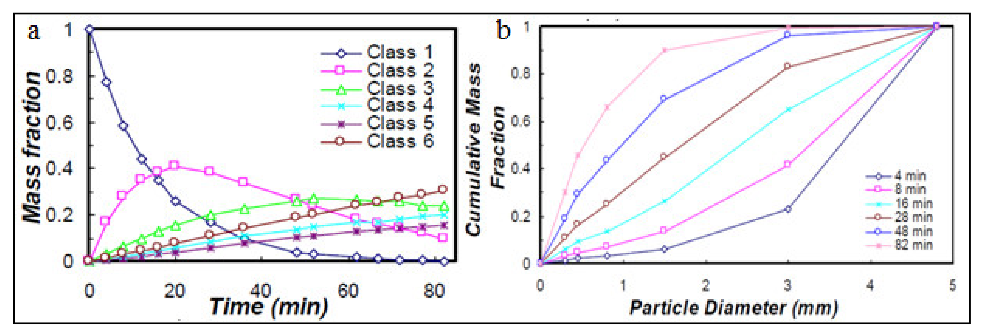
and that would be the space in which the AR is determined. Both the feed and the product streams should be represented as points in dimensional space. Figure 1 is an illustration of how experimental data can be represented. The grinding profiles can be grouped into mass fractions m₁, m₂ and m₃, where m₁ is termed the feed size fraction, m₂ the middling size fraction and m₃ the fines size fraction. The margins of the mass fractions are dependent on the objective function to be achieved. For example, if we consider m₁ to consist of size classes 1 and 2, m₂ to be made of size classes 3 to 5 while size class 6 constitutes m₃, we can clearly define our objective function.

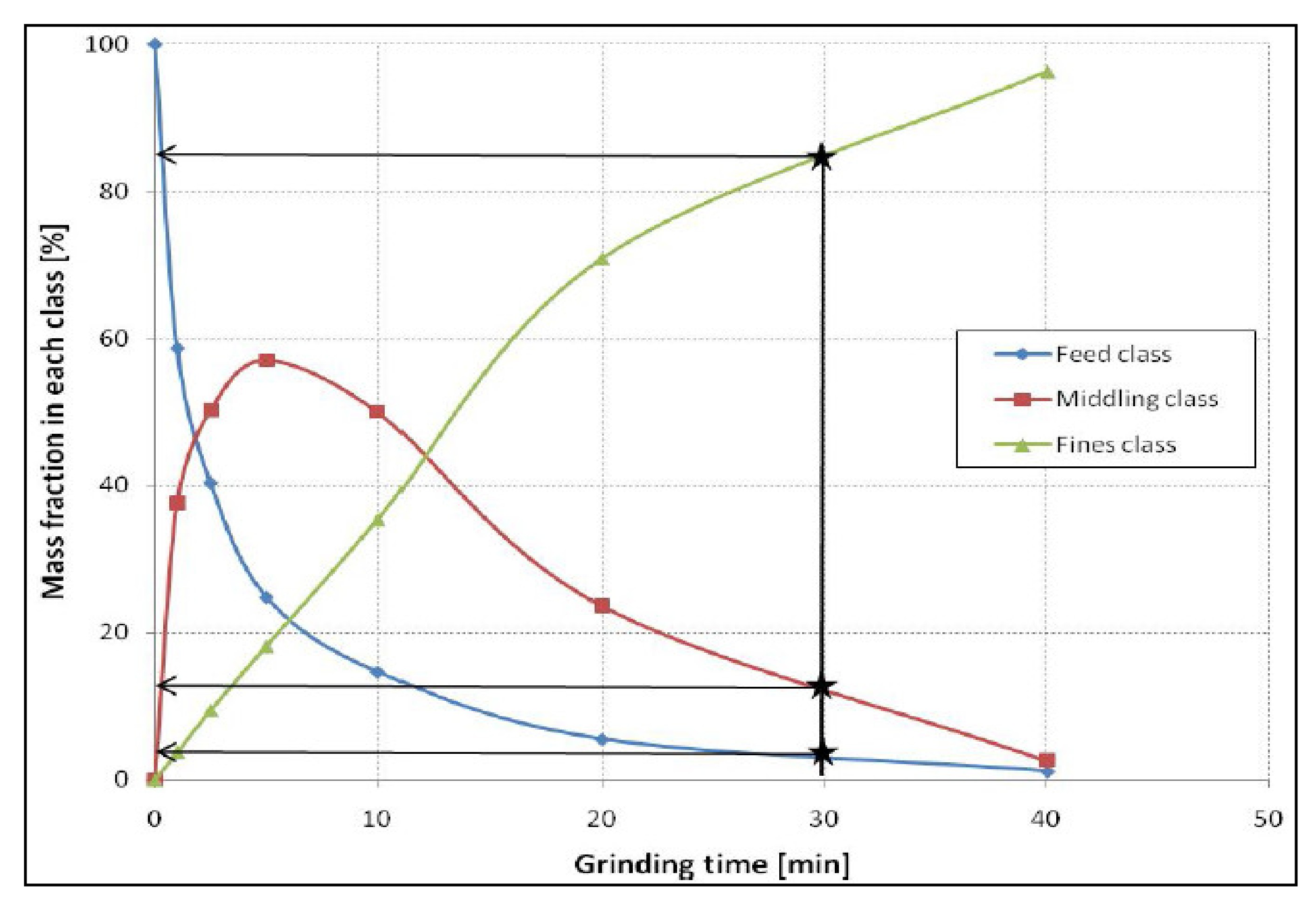
Figure 2 illustrates the mass fractions of m₁, m₂ and m₃. If the objective is to maximize the production of the middling (m₂), then from the AR analysis illustrated here, we can interpret the graph to determine the optimal grinding time.

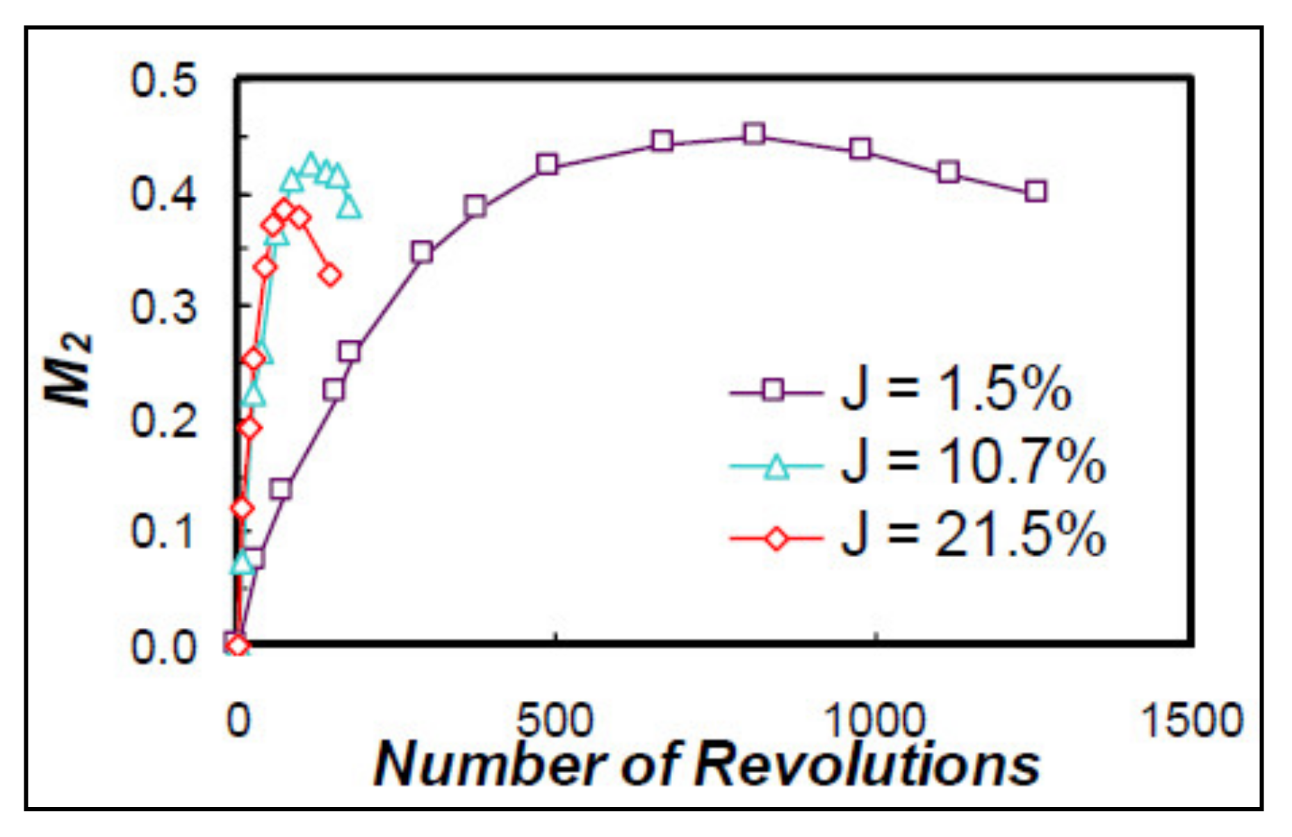
We can then extend this analysis to compare the discrete maxima of m₂ obtained under different specified operating conditions. An example of different maxima of m₂ obtained with dissimilar media charges (J) at a single speed is illustrated in Figure 3.

Now that mass fractions at different grinding times have been clearly explained, the next step is to present the data in a final AR format. Figure 4 shows how particle size distributions (PSD) can be connected with grinding time. In this plot, the boundary curve describes the processes used and can be interpreted in terms of pieces of equipment (implicitly identifying the equipment required for best performance). Mass fractions external to the AR defined by its trajectory cannot be achieved. The turning point of the curve isolates an optimum solution when the objective is to maximize the mass in size class 2 (m₂). This solves the optimization problem and provides the process control policy needed to achieve that objective.

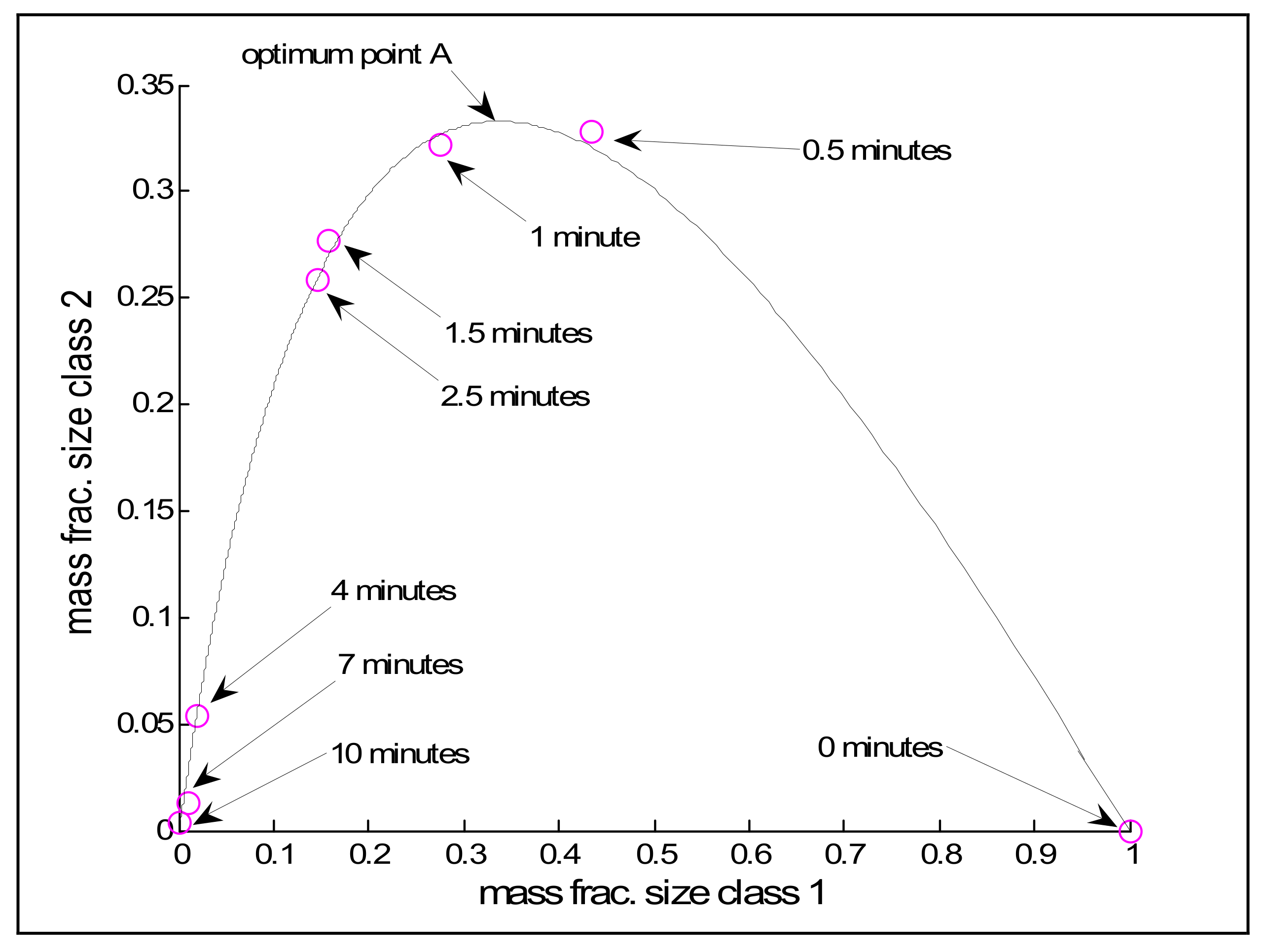
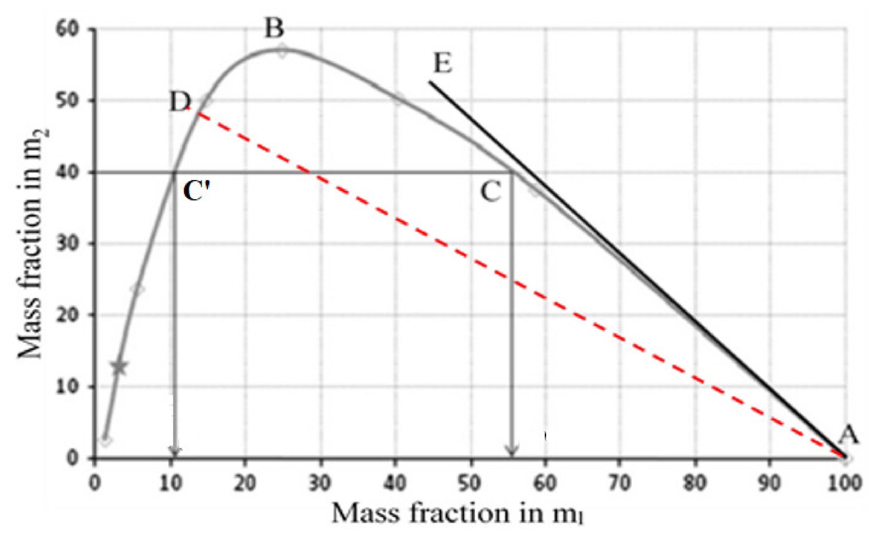
To explain further and clarify the PSD as a single trajectory in Figure 4, Figure 5 is presented which shows a plot of m₁ vs. m₂ size fractions. In Figure 5, point A represents the feed of the mill and point B is the turning point of the curve which isolates an optimum solution when the objective is to maximize the production of m₂, hence solving the optimization problem in the system.

At point C, 45% of the feed material has been broken into m₂ and m₃, which then comprise 40% and 5% in the product stream, respectively. In the curve is also shown point C′ which has the same concentration of 40% of m₂ when 90% of m₁ is milled. The amount of m₁ which remains in the system at C is 55% and m₃ is (100 − m₁ − m₂) = 5% whereas at C′, m₁ which remains in the system is 10% and m₃ is (100 − m₁ − m₂) = 50% as determined by mass balance. Thus, more fines are produced at point C′ than at point C even if the concentration of m₂ in the stream is the same at both points.

Line AE is a 45° line and breakage along that line corresponds to the breakage of material during the grinding process from m₁ to m₂ only, with no production of unwanted fines (m₃). Conversely, the line from A to the origin corresponds to the breakage of material in m₁ directly to m₃, thus producing no m₂. To maximise the rate of producing m₂ from m₁, the grinding process should be operated as close to line AE as possible. Thus, the initial breakage at A produces mainly m₂ and little m₃ for every quantity of m₁ broken and has the maximum rate of breakage of m₁ to m₂.

The power of AR lies in its ability to determine the performance of the optimal circuit as well as the operational conditions to be used in the optimal process circuit. It also defines process targets accurately, which in turn permits the engineer to measure the actual process efficiency against a theoretical target. Khumalo et al. [5] were able to validate their AR predictions by showing a good fit between their calculations and their experimental results. They then investigated the theoretical implications of their basic model for different specific energy inputs [6] and successfully used AR analysis to optimize milling circuits that also include the classification of particle sizes [7]. The main focus of the work done by Khumalo and his colleagues [5,6,7] was on achieving the desired product with optimal use of energy.

Metzger et al. [8] used the same AR analysis technique but applied it to a different parameter: optimizing the total time of operation. They found that the AR could be used to determine optimal policies to reduce milling processing time. Katubilwa et al. [9] also used the AR to analyse the effect of ball size on milling, based on the experimental data they had collected from milling coal. They confirmed the generally accepted trend that grinding balls of small diameter tended to promote the production of fine particles at a higher rate than can be achieved by large balls. Mulenga and Bwalya [10] then used MODSIM^® (Academic Version 3.6, Mineral Technologies Inc, Salt lake City, UT, USA) to simulate an industrial mill and generated data which they used to analyse ball filling, slurry concentration and feed flow rate within the AR framework.

Danha et al. [11] used the AR to optimise the size reduction of a platinum group minerals (PGM) ore in a laboratory grinding mill, specifically focusing on the effect of slurry concentration on the product size distribution (PSD). Using the same technique, they were also able to determine the optimal grinding time and energy needed to achieve the maximum production of the desired size fraction. In the same work, they also revealed that mixing is desirable in certain instances to maximise the production of a given size fraction, especially if the m₁ vs m₂ trajectory is concave. Danha et al. [12] then investigated the breakage behaviour of a bed of particles using AR to identify the optimum operating parameters. The objective function of the work was to minimise energy usage in the breakage process whilst maximising the production of the desired size fraction. Thus, they used the AR technique to determine the ball size needed to achieve the objective function. The work also looked at mixing as an important fundamental process needed in the event of maximising the productions of fines.

Hlabangana et al. [13] further explored the technique by applying it to optimise the grinding time required to achieve the maximum production of the desired size fraction. Ball and powder filling was at the centre of their optimisation scheme. Later on, Hlabangana et al. [14] used the AR to optimise the milling and leaching of low-grade ore. They particularly maximised the material recovered whilst minimising the cost associated with the recovery. The AR of the 3D plots enabled the authors to achieve all possible recoveries from different milling and leaching times. This was achieved through overlaying a contour plot of the objective function on the 3D plot. Using the laboratory scale mill, Hlabangana et al. [15] conducted tests and explored the effect of varying the feed and grinding media size distribution on the product fineness using AR. After that, Hlabangana et al. [16] used the AR to analyse and optimise the impact energy on a bed of PGM, particularly focusing on the effect of drop weight shape on the product fineness.

Mulenga and Chimwani [17] extended the use of the AR from batch milling to continuous and full-scale milling using Austin et al.’s [18] scale-up procedure, then optimised the residence time of particles in the mill. Their investigation was limited to the plug flow and well-mixed mill transport models without exit classification. The AR of the desired product size was identified as well as the pivotal operational parameters. Using the same scale-up scheme, Chimwani et al. [19] demonstrated the ability of AR to optimise milling circuits at an industrial scale by assessing the effect of ball sizes and power draw on the production of the desired size fraction. The authors scaled up laboratory data to a preselected industrial mill of known parameters and specifications and demonstrated the ability of AR to optimise milling at that scale. Chimwani et al. [20] then later took advantage of the transport model developed for an industrial mill by Makhokha et al. [21] to determine the optimal residence time of ore in the ball mill using the AR. The authors evaluated the energy requirements of the mill at that residence time to produce a maximum amount of the desired fraction. This work also explored the effects of the operational speed and mill filling on the particle residence time.

Chimwani et al. [22] used the AR technique to explore the effect of ball mixture on the production of the floatable size range applicable to a platinum-bearing ore. The authors generated a simulation program that comprises the grinding circuit and ball wear models, which were used to determine the optimum make-up balls needed to produce the maximum amount of the desired size range. Chimwani and Hildebrandt [23] then optimised an open mill circuit using the AR technique in terms of the energy consumption needed to produce a given size range. The approach in that work was slightly different from the rest in that an operating region that comprised the best combination of mill speed and ball filling that produced the highest amount of floatable size fraction with minimum energy consumption was determined from the optimisation scheme. Two years later, Chimwani et al. [24] optimised the production of the desired size range in a grinding mill through tailoring the feed size distribution. The AR technique was utilised to analyse the data simulated using the population balance model and the analysis revealed that the milling process is efficient only to a point where the rate of producing the desired product size is greater than or equal to the rate of producing unwanted fines.

Emmanuel et al. [25] used the AR technique to optimise impact energy and particle size during the breakage of a bed of olivine particles, demonstrating that the technique is applicable in sustainable soil stabilization projects. Using the technique, they found spherical drop weights to be more influential in maximising the production of the desired size fraction.

As has been shown above, a considerable amount of work has been done by researchers over the years to apply the AR methodology to comminution processes with important insights drawn from the results. On the one hand, some of the results from the AR analysis confirmed what is already known in the comminution world whilst on the other hand, some results revealed things that were concealed by other analysis techniques yet important in the optimisation of comminution circuits. This review thus helps to shed light on the important insights drawn from the AR analysis technique as applied to tumbling mills, to encourage its adoption by the generally conservative mining industry.

2. The AR Application in Comminution

To effectively apply this graphical analysis technique to optimise various operating conditions of comminution circuits and unlock its potential, several researchers have coupled it with the population balance model [7,9,19,20,22], with insightful information drawn from the work. The population balance model is a size-mass balance that takes into account the selection and breakage functions resulting in the full description of the grinding process. If a size-mass balance is performed for particular size i, the rate of production of size i material equals the sum of the rate of appearance from breakage of all larger sizes minus the rate of the disappearance by breakage. This is symbolically expressed as follows [18]:

$$\frac{d{w}_i\left(t\right)}{dt}=-S_i.w_i\left(t\right)+{\displaystyle \sum _{j=1}^{i-1}{S}_j.b_{ij}.w_j\left(t\right)}$$

(1)

where $S_j{b}_{ij}{w}_j\left(t\right)$ is the rate of appearance of size i material produced by the fracturing of size j material; $S_i{w}_i$(t) is the rate of disappearance of size i material by breakage to smaller sizes; $S_i$ is the selection function of the material considered to be of size i; $w_j\left(t\right)$ is the mass fraction of size i present in the mill at time t; and $b_{ij}$ is the mass fraction arriving in size interval i from breakage of size j. S_i is the selection function that represents the rate of breakage of particles of size x_i.

Austin et al. [18] proposed the following empirical model to define the variation of the selection function with particle size:

$$S_i=a.x_i^{\alpha }.Q_i=a.x_i^{\alpha }.\frac{1}{1+{\left(\frac{x_i}{\mu }\right)}^{\mathrm{\Lambda }}}$$

(2)

where x_i is the maximum limit in the screen size interval i in mm; Λ and α are positive constants that are dependent on material properties; a is a parameter dependent on mill conditions and material properties, which indicates how fast the grinding is; µ is a parameter dependent on mill conditions; and Q_i is the correction factor accounting for abnormal breakage.

The distribution of fragments produced by breaking size i before re-breakage occurs is called the primary daughter fragment distribution b_ij. It is the ratio of mass from size class j reporting to size class i [18]:

$$b_{ij}=\frac{\mathrm{mass} \mathrm{of} \mathrm{particles} \mathrm{from} \mathrm{class} j \mathrm{broken} \mathrm{to} \mathrm{size} i, t\to 0}{\mathrm{mass} \mathrm{of} \mathrm{particles} \mathrm{of} \mathrm{class} j \mathrm{broken}, t\to 0} \mathrm{where} i < j$$

A more convenient way of describing the breakage function is to represent it in cumulative form

$$B_{ij} = {\displaystyle \sum _{k=n}^i{b}_{kj}}$$

(3)

where B_ij is the sum of the fraction of material that is less than the upper size of size interval i resulting from the breakage of size j material. b_kj is the cumulative breakage function of particles of size xj reporting to size class i.

To relate the cumulative breakage function to particle size, the following empirical model can be used [18]:

$$B_{ij} = {\mathrm{\Phi }}_j{\left(\frac{x_{i-1}}{x_j}\right)}^{\gamma }+ \left(1-{\mathrm{\Phi }}_j\right){\left(\frac{x_{i-1}}{x_j}\right)}^{\beta }$$

(4)

where β is a parameter characteristic of the material used, the value of which is generally greater than 2.5; γ is a material-dependent parameter, the value of which is typically found to be greater than 0.6; and Φ_j is a material-dependent parameter representing the fraction of fines that are produced in a single fracture step. Its value ranges from 0 to 1.

The breakage and selection function parameters determined were used within the PBM framework [19,20,22] and the academic version 3.6 of MODSIM^® (Mineral Technologies Inc, Salt lake City, UT, USA) [10] to generate data from simulations at different operational parameters both at laboratory and full-scale milling. All the simulations had a similar objective of generating data for analysis using AR. This review thus provides a yardstick for determining the difference between the results obtained from the AR analysis and what is conventionally known in comminution, for optimum operational parameters of different comminution devices and test equipment.

3. Different AR Application Scenarios

It is important to understand that AR is an optimisation tool that uses an approach which is equipment independent. As mentioned in the foregoing sections, its application has been to a greater extent on ball mills. The ball mill is composed of a number of operational parameters. In some instances, researchers have focused on a particular operational parameter [8,9,11,13,14,15,16,17,19,20,22,23,24,26] whilst in some cases, the optimisation scheme focused on all parameters at once to achieve a given objective function [19]. This makes grinding materials in a manner conducive to achieving the objective function key to good mineral processing. The engineer who controls the milling operation thus needs to strike a balance between reducing the size of the particles and minimizing over-grinding (to maximize efficiency). On the one hand, under-grinding yields a product that is too coarse and has a degree of liberation too low to be economically feasible when the downstream separation process has been completed. Over-grinding, on the other hand, tends to reduce the materials below the size required for most efficient separation and additionally results in unnecessary waste of energy.

These considerations have prompted several researchers to investigate the milling process in detail, studying milling parameters such as ball size, slurry filling, residence time distribution, grinding media filling and media shape, and subsequently to make various recommendations to ensure the efficient operation of ball mills. These systematic studies were carried out by Kelsall et al. [27,28,29,30,31] and other pioneers in the field, whose recommendations established a basis that researchers such as Austin et al. [18] and Yekeler [32] have built upon to propose models that describe the effects of typical grinding parameters on the milling process. In tumbling ball mills, the rate of breakage and overall mill performance is affected by, among other factors, fractional ball filling (J), the fraction of critical speed (${\varphi }_c$), the fraction of the mill volume filled by powder (f_c), powder filling (U), solids concentration, ball and feed size distributions.

With the introduction of the AR optimisation tool, researchers looked again into the optimisation paradigm from the perspective of the graphical analysis tool. In the subsequent section, a detailed review is given on the application of the technique on different milling operational parameters.

3.1. The Fractional Ball Filling

Fractional ball filling (J) is conventionally expressed as the fraction of the mill volume filled by the ball bed at rest, assuming a formal bed porosity of 0.4. It can be expressed as [18]:

$$J=\frac{\left(\frac{\mathrm{mass} \mathrm{of} \mathrm{balls}}{\mathrm{ball} \mathrm{density}}\right)}{\mathrm{mill} \mathrm{volume}}\times \frac{1.0}{\left(1-0.4\right)}$$

(5)

Metzger et al. [8] investigated the effect of the grinding media filling (J) and multiple speeds on the breakage of silica sand particles using the AR graphical analysis. They used a benchtop laboratory ball mill loaded with grinding media. The authors found that the single mill speed (${\varphi }_c$ = 0.21) and the lowest media filling of J = 1.5% produced a maximum amount of m₂ compared to J = 10 and 21.5%. Hlabangana et al. [13] also found the media filling of J = 4% to be a better policy for optimising the mill after comparing it to J = 10.7% from the laboratory experiments performed on silica and gold ores.

These results contrasted those of Austin et al. [18] and Ozkan et al. [33] which suggested that energy is most efficiently used at ${\varphi }_c$ = 0.75 and J = 40% but in large-scale ball milling. This is on account of a widely held belief that as the mill draws maximum power, the rate of breakage also gets to the maximum. Motivated by that disparity, Metzger et al. [8] performed experiments with the parameters of ball filling (J = 31.5%) and mill speed (${\varphi }_c$ = 0.71) but the process was not optimised as expected; rather, a lower amount of the desired size was produced.

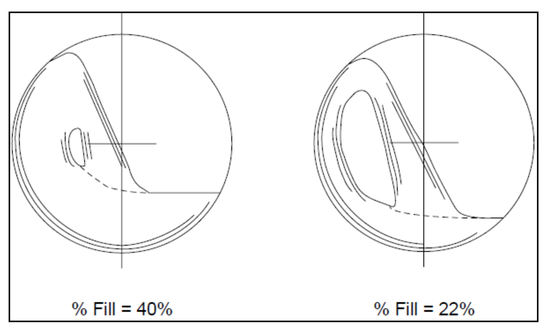
However, Fortsch et al. [34] reported a slightly lower media filling. The authors used the under-loading multiplier concept which is pronounced by the hole or gap in the middle of the charge as the mill is turning. They then reported that operating a ball mill at 75% critical speed and a 22% charge level creates a higher cataracting region than at 75% critical speed and 40% charge level. The multiplier concept is shown in Figure 6.

They also observed that cascading action provides the highest grinding efficiency because of the high total surface area exposed to contact. Finally, Fortsch and his colleagues argued that as the ball filling is increased, the breakage rate initially rises to a maximum and then decreases.

In their quest to extend the AR methodology to full-scale milling and, also to understand the cause of the difference between Metzger et al. [8] AR analysis results from lab data and that of Austin et al. [18] and Ozkan et al. [33] from large scale milling, Mulenga and Chimwani [17] used the Austin et al. [18] scale-up procedure to scale laboratory data to an industrial continuous milling. Although the main objective was to optimise the residence time in terms of the plug-flow and well-mixed transport models, their work showed that higher ball fillings led to the faster production of the desired size fraction. In particular, the recommended range of ball filling by Mulenga and Chimwani [17] was J = 25%–30% for the range of J = 20%–35% investigated, which was not far from that proposed by Fortsch et al. [34]. However, the authors observed that the high-power draws and throughputs achieved when high ball fillings were used require an extensive inquiry into the possibility of a trade-off between throughput and mill power draw.

In that light, Chimwani et al. [19] scaled up data obtained from laboratory batch milling of a platinum ore using empirical models to an operational industrial mill on which some plant survey had been conducted. Higher media filling of J = 40% was presented in that work, confirming what is traditionally acceptable in milling practices under which most concentrators operate. These results were slightly different from what Mulenga and Chimwani [17] found of J = 20%–30%. The difference is perhaps owing to the approaches used. In the former, the media filling was optimised independently of other operational parameters or other parameters were held constant whereas, in the latter, all the parameters were optimised at once to maximize the production of m₂ (−75 + 9 µm). To optimise many parameters at once, a search algorithm was generated to search for the optimal values of mill operational parameters J, U, d and ${\varphi }_c$ that would produce the highest amount of the desired size fraction. The calculation procedure utilised the Matlab^® (Version R2017a/15, Natick, MA, USA) function “fmincon” which uses a sequential quadratic programming method. The method solves a quadratic programming sub-problem and an estimate of the Hessian of the Lagrangian is updated after each iteration by globally converging all the unknown parameters simultaneously and not adjusting them one at a time.

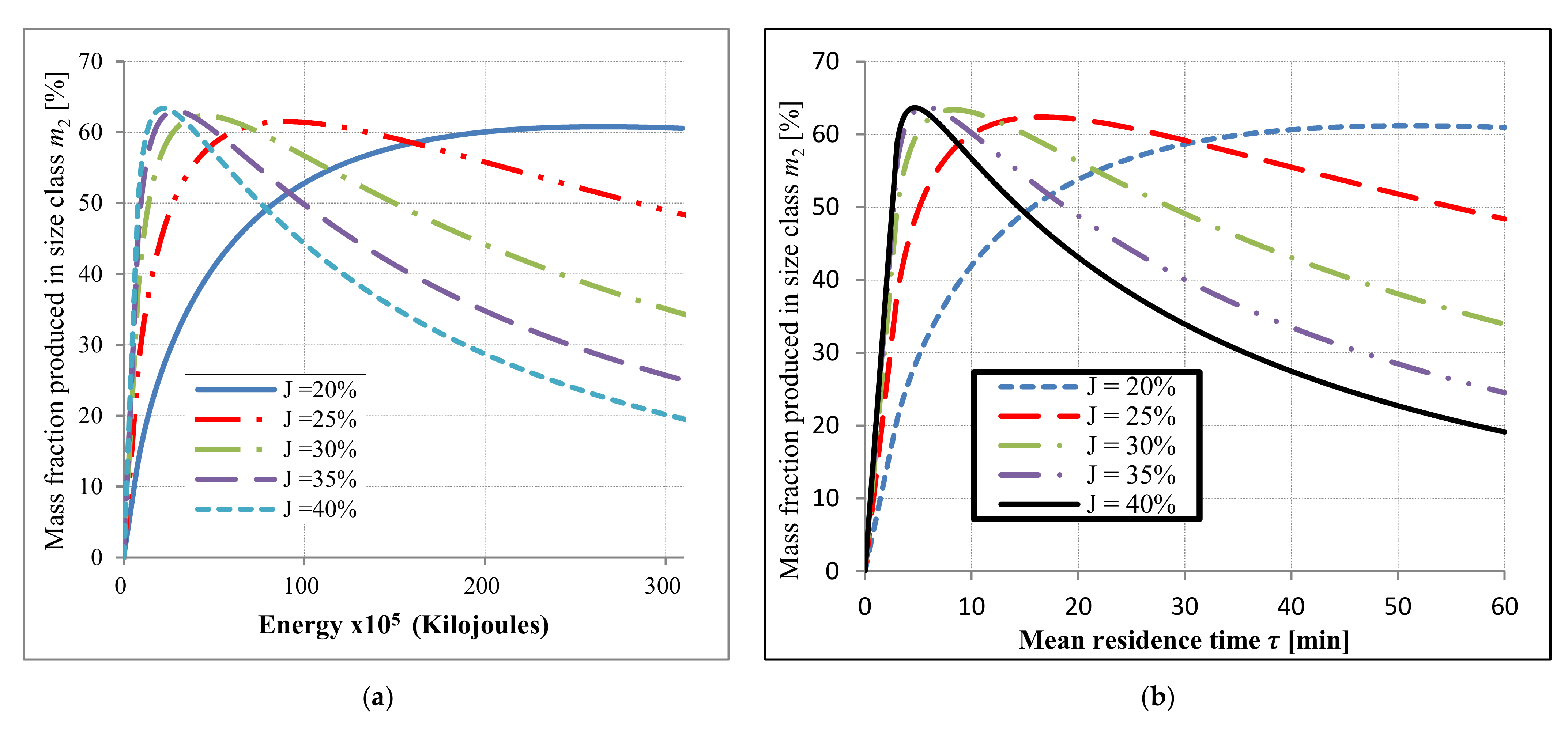
Later on, Chimwani et al. [20] extended the enquiry to the use of the AR technique, determining the optimal residence time of ore in the industrial ball mill. In earlier work [17,19], the assessment was limited to the plug flow and fully-mixed mill models. Later, they used a tank in series model after determining that it was more realistic and assessed the energy requirements at different ball filling to maximise the production of the desired particle size fraction for floatation. It was found that the highest amount of material in the −75 + 9 µm size range was achieved at J = 35% but the residence time was optimised at J = 40%. In terms of the energy assessment, operating at a higher ball filling of J = 40% was found to be a better choice if the mill is to be optimised as shown in Figure 7. These results were confirmed by Mulenga and Bwalya [10] who, through data generated from the simulation of the same industrial mill using MODSIM^®(Academic Version 3.6, Mineral Technologies Inc, Salt lake City, UT, USA), found optimum ball filling to be within the range of 35 to 40%.

3.2. The Rotational Speed

The mill rotational speed is normally specified as a fraction of the critical speed ${\varphi }_c$. The critical speed is the theoretical rotational speed at which balls centrifuge on the mill case and do not tumble. This is given by [18]:

$$\mathrm{Critical} \mathrm{speed} {\varphi }_c, \mathrm{rpm}=\frac{42.2}{\sqrt{D-d}}$$

(6)

The rotational speed affects the product size distribution and how fast the shell liners wear. Shoji et al. [35] found that the industrial mill rotational speeds in use were 70%–80% of critical speed for a ball mill with effective lifters. The typical operational philosophy is to run the mill at the speed at which the trajectories followed by the balls are such that the descending balls fall on the toe of the charge and not on the liners. This is attributable to concordant studies that demonstrated that low speeds give rise to abrasive grinding owing to the cascading of the balls, which in turn results in finer grinding and increased liner wear. At higher speeds, cataracting tends to dominate the grinding process, resulting in coarser end products and reduced liner wear. Further increase of the mill speed to close to 100% leads to centrifuging; the media are carried around in an essentially fixed position against the shell [36]. Understanding that there is no cast in stone mill rotational speed which is a one size fits all for the mill optimisation, subsequent research was conducted using AR analysis techniques to optimise grinding mills in terms of the operational parameter and it is interesting to assess the results against the traditionally acceptable practice.

First to carry out the enquiry was Metzger et al. [8] who then suggested through AR analysis that energy is most efficiently used at low mill rotation rates to produce the maximum amount of m₂, thus contradicting what is traditionally known, which is running the mill at ϕ_c = 75%. The authors observed that operating the mill at ϕ_c = 3% as shown in Figure 8 produced the largest amount of the desired size fraction with efficient energy utilisation, but after the longest grinding time. Thus, Metzger et al. [8] proposed that instead of running the mill at a single rotational speed, the ore should be milled in a series of mills where the first mill can operate for a shorter period at a higher energy input followed by grinding in the subsequent mill at a lower energy input for a longer time. This, as per their conjecture, helps to utilize the overlapping grinding profiles and achieve a given objective function of producing the amount of the desired size range in half the time taken to produce that material in a single rotation speed.

Upon extending the AR technique from the batch to continuous milling, Mulenga and Chimwani [17] found that the critical speed of ϕ_c = 70% recorded the shortest time during the residence time optimisation. That rotational speed also produced the maximum amount of m₂. Although the results confirmed what Shoji et al. [35] also observed, the authors acknowledged the use of simplified flow models which were unrealistic in essence. Despite the achievement of the objective function of the study, Mulenga and Chimwani [17] proposed the use of a more comprehensive simulation model that integrates all the relevant aspects of milling operations for the generation of more relevant data. In that breadth, Chimwani et al. [19] scaled up laboratory data to an industrial mill and found that ϕ_c = 40% produced the highest amount of the desired size fraction which was −75 + 9 µm. Even the search algorithm developed to optimise the ball filling, interstitial filling, critical speed and ball diameter whilst maximising the production of the desired size fraction confirmed the critical speed of ϕ_c = 40% to be optimal. This disagreed with the common practice which recommends 75% of critical speed as optimal.

To further explore the output limits of a system in terms of the rotational speed, Chimwani et al. [20] stretched the enquiry of the AR technique analysis to the realistic model. The results obtained confirmed what the same authors found in their earlier work, that the critical speed of 40% produced the maximum amount of the desired size fraction (−75 + 9 µm) with minimal energy expenditure. Later, Chimwani and Hildebrandt [23] explored the possibility of determining the optimal conditions in terms of energy consumption that optimises the production of the desired size fraction as dictated by the ball filling and mill speed. The authors used a different approach from the one used in their earlier work. The new approach optimised the circuit based on a set output rate of the desired size fraction. The output rate was set based on the lower boundary of the AR which was slightly lower than the peak value. The difference between the amount of the desired size fraction at the peak and that on the lower boundary of the AR was found to be insignificant whereas that of the energy expended to produce the amount of the desired size fraction at the peak and that at the lower boundary was very significant. For further clarification, the analysis of the attainable region was performed using contour plots, which unveiled further opportunities to fine-tune the optimization paradigm. The work of Chimwani and Hildebrandt [23] showed that it is possible to sacrifice less than 1% of m₂ produced to save energy by more than 30%. Operating the mill speed at 40% critical speed instead of the conventional practice of operating between 70% and 80% was confirmed to be the best practice since it saves energy expended by 15%. This, whilst confirming the earlier findings by Chimwani et al. [20] about rotational speed, shows that mill speed is an important factor in the optimization of milling circuits.

3.3. Mill Filling by Powder

The fraction of the mill filled by powder (f_c) is expressed as the function of the mill volume filled by the powder bed, using a formal bed porosity of 0.4. This is calculated using Equation (7). The fraction of the mill filled by powder (f_c) must be determined for every mill operation in which a different J is used since the mill should not be under- or over-filled. Under-filling the mill leads to energy wasted in steel-to-steel contacts, which produces little breakage, but instead, unwanted material wear. Over-filling the mill, on the other hand, leads to an effect called powder cushioning, which impedes the efficiency of the breakage action. That is why it is imperative to fill the mill with an appropriate volume of powder. The fraction f_c of the mill to be filled by powder can be calculated as follows:

$$f_c = \frac{\left(\frac{\mathrm{mass} \mathrm{of} \mathrm{powder}}{\mathrm{powder} \mathrm{density}}\right)}{\mathrm{mill} \mathrm{volume}}\times \frac{1.0}{0.6}$$

(7)

A similar definition applies to the slurry, provided that the density of powder in Equation (7) is replaced by an appropriate density of slurry.

In order to relate powder loading to ball loading, the formal bulk loading of powder is compared to the formal porosity of the ball bed [18]. This way, the notion of powder filling (U) can be introduced, that is, the fraction of the spaces between the balls, at rest:

$$U = \frac{f_c}{0.4J}$$

(8)

Austin et al. [18] reported that the values of U between 0.6 and 1 will generally give the most efficient breakage in the mill. The authors attributed the small breakage rates obtained with a low powder filling to the little collision spaces between the balls that would be filled with powder. Previous works [33,37,38] have shown that the grinding rate is affected in the same manner regardless of whether it is the slurry or powder that fills the interstices of the mill bed. Latchireddi and Morrell [39] and Tangsathitkulchai [38] proposed U = 1 as the way to ensure efficient milling. Chimwani et al. [19] also confirmed the same value from their AR analysis of scaled-up data. The authors found this value both when they optimised the operational parameter solely and when optimised it together with other parameters using the search algorithm.

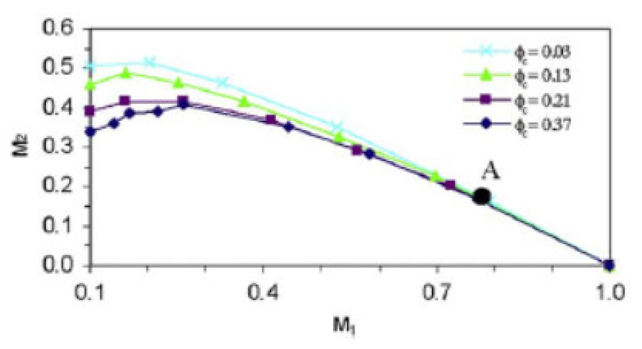
Intending to reduce the grinding time required to maximise the production of material in the desired size fraction (−150 + 75 µm), Hlabangana et al. [13] used the AR technique to optimise the grinding process in terms of powder filling. Their results revealed that at U = 1, the rate of production of the desired size is maximised, confirming what the previous researchers have found regardless of whether the AR analysis technique was used or not. Later, Hlabangana et al. 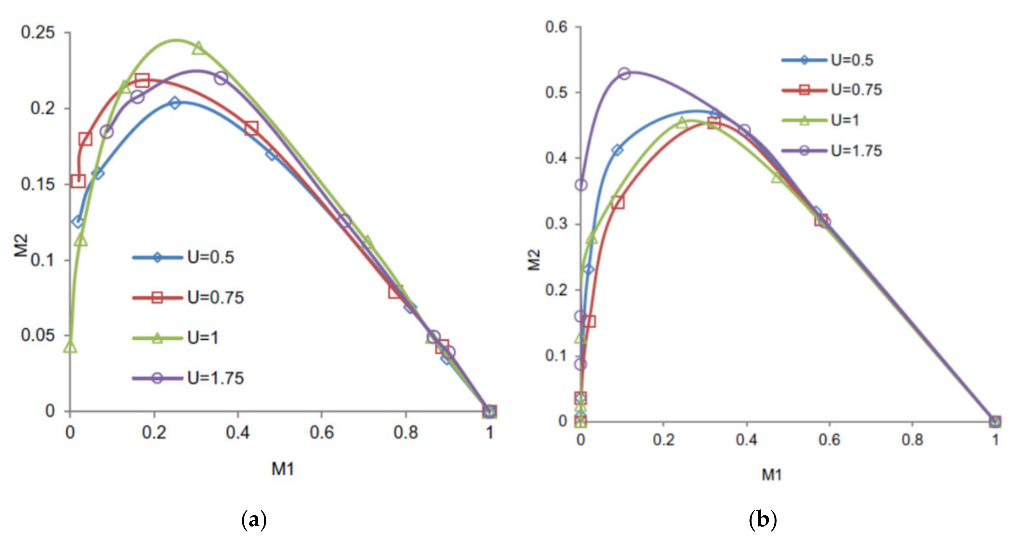[40] continued with their enquiry about the effects of powder filling on the production of the desired size fraction using the AR technique and demonstrated that the optimum powder filling for a given grinding action is related to the limits of the product specification. The authors thus showed that U = 1 was the optimum value for maximising the production of −150 + 75 µm whilst U = 1.75 was the optimum for producing −850 + 150 µm as shown in Figure 9. This encouraged the authors to propose the use of mills in series with different U values as long as the product requirements in terms of particle sizes are different. However, their results confirmed previous suggestions of U = 1 for similar product requirements.

3.4. Ball Diameter

Several published research studies have shown concordance in finding that fine particles are ground effectively by small balls, because of the increase in the rate of ball-on-ball contacts per unit time [18,41,42,43,44]. Furthermore, if a representative unit volume of the mill is considered, the number of balls in the mill increases, as 1/d³. On the other hand, larger balls have been found to do a better job as far as the milling of hard ores and coarser feeds are concerned, since high impact energy is required to break them [41]. To add to the existing literature about the ball size effect on milling kinetics, some researchers resorted to assessing it through the lenses of AR analysis.

First to undertake the analysis was Katubilwa et al. [9], who through a theoretical inquiry utilised the AR technique to investigate the effect of ball diameter on milling kinetics. Their objective function was slightly different from the one pursued in most research work concerning the AR analysis, that is, to maximise the production of the middling size fraction commonly known as m₂. For Katubilwa et al. [9], the objective function was to maximise the production of the material less than 75 µm, which is basically m₃. The ball sizes under investigation were: 10, 20, 30, 40 and 50 mm. Those balls were used on three different feed sizes: a coarse feed 26,500–22,400 μm, a medium feed 6700–4700 μm, and a fine feed 600–425 μm. The AR analysis showed that when grinding a coarse feed, the 20 mm ball size produced the highest amount of m₃ for any amount of m₁ ground, but the story changed for a medium feed where 10 mm ball produced the highest amount of m₃. For the finest feed, the curves were superimposed, and that showed that there is a feed size beyond which ball size ceases to matter from an AR analysis point of view. The general conclusion from that work is that smaller diameters were more effective at producing materials under 75 μm although they are shunned in the industry because of the cost. The authors also acknowledged that the effect of ball size could be different for some other operating conditions and that a mixture of balls of different diameters might be able to take advantage of both small and large media confirming what is conventionally known about the subject. The observation of the mixture of balls as a better option was later emphasised by Mulenga and Bwalya [10].

To shed more light on the subject, Metzger et al. [45] investigated the effect of grinding media size among other parameters on the optimal production of the desired size fraction m₂. The authors only compared how the 44.5 mm and 25.4 mm ball diameters differ in grinding ability of feed size 5600–4000 μm. They found 44.5 mm diameter ball sizes to optimise the production of m₂ which was the desired size fraction. The results of Katubilwa et al. [9] and that of Metzger et al. [45] are not comparable owing to different objective functions pursued in each work.

To bring more insights into the subject, Mulenga and Chimwani [17] through their introduction of AR to continuous milling, investigated the effect of ball sizes; 10, 20, 30 and 40 mm on the production of the desired size fraction (−75 + 9 μm). The results show that smaller balls promote a faster production of the desired size fraction. Since the results confirmed the patterns reported by Austin et al. [18] and Napier-Munn et al. [41], they confirmed the widely accepted theory pertaining to the effects of ball size in milling, which requires ball diameter to be tailored to the target product. In the same vein, Chimwani et al. [19] scaled up the laboratory data to a full industrial mill and observed that as the ball size decreased, the maximum achievable mass fraction of the desired fraction (−75 + 9 µm) decreases as well. Their investigation only covered ball sizes 20, 30 and 40 mm and from that investigation, 40 mm balls were found to produce the highest amount of the desired size fraction. The authors also confirmed the same results when they used a search algorithm scheme to optimise all the parameters at once. Through their simulation of a full-scale mill with a realistic model, Chimwani et al. [20] demonstrated that residence time is largely dependent on ball diameter and that correct adjustment of ball diameter is needed for the optimisation of the residence time. However, the assessment of ball size using AR analysis is still sparse from an energy perspective.

Chimwani et al. [22] investigated the make-up ball charge that would guarantee maximum production of the floatable size range applicable to platinum-bearing ore using the AR technique. Their results revealed 20 mm balls to constitute make-up balls that produced the highest amount of (−75 + 9 µm) which was the desired size fraction (98.3%). This was followed by 40 mm balls as a make-up charge which produced m₂ of 94.6%. The results from the AR analysis in that work confirmed those found by Bwalya et al. [46]. The authors went on to argue that despite 20 mm balls producing the maximum amount of the desired size fraction, it was advantageous to charge 40 mm balls as make-up charge owing to the insignificant difference in the amounts of m₂ produced which was just 3.7%.

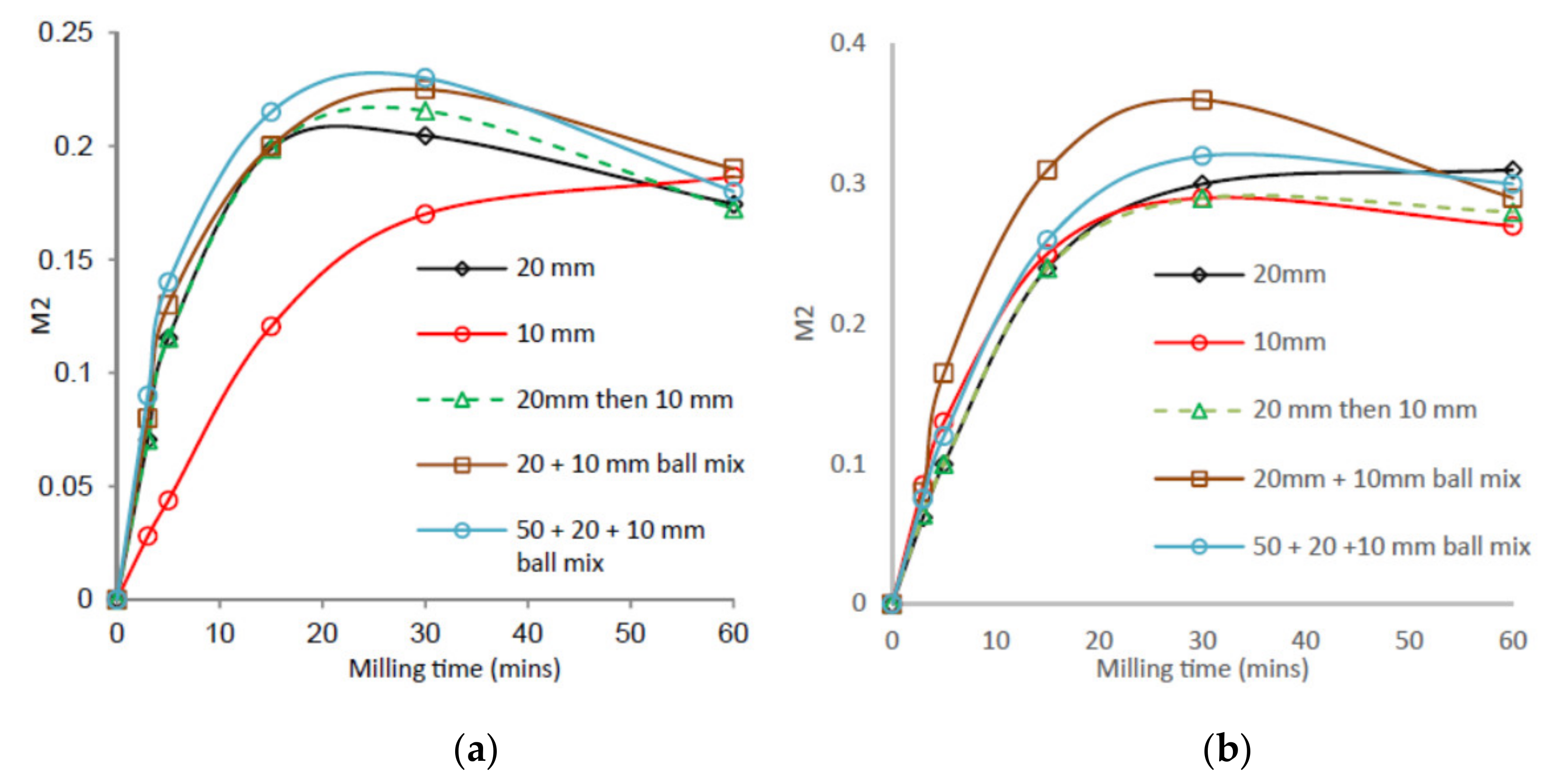
Hlabangana et al. [15] used the AR analysis to investigate the effect of ball size and feed size distribution on the production of the desired size fraction. The investigation focused particularly on the mixture of ball sizes rather than one size as investigated in other previous work. The ball mixtures investigated, which constitutes the combinations of 50, 20 and 10 mm and that of 20 and 10 mm ball sizes, were investigated on feed size classes −1700 + 850 mm and −1180 + 850 mm. Their AR analysis revealed that the three-ball mixture maximised the production of m₂ (−150 + 75 µm) from the grinding of a coarser size whilst the binary ball mixture maximised the production of the desired size fraction from milling the finer feed, as shown in Figure 10.

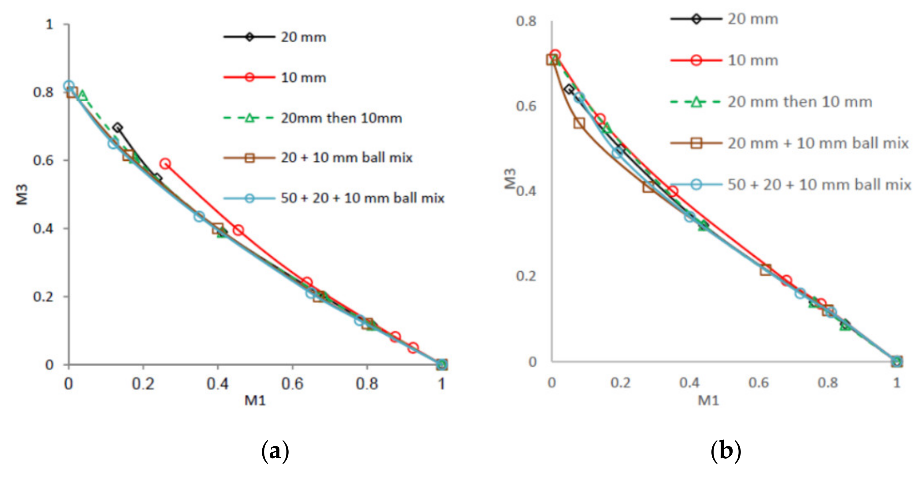
When the enquiry was extended to the optimisation of m₃, the results presented in Figure 11 show that the three-ball diameter mix produced fines at the fastest rate for the coarser feed whilst the binary mixture performed better than its rival for the finer feed although overall, it was a 10 mm diameter ball which maximised the production of m₃ for that feed size. The results from Hlabangana et al. [15] reinforce that the grinding media diameter should be matched according to the feed and desired product size distributions.

In their quest to optimize the impact energy of breaking particles bed, Danha et al. [12] used AR analysis to assess the breakage behaviour of a bed of silica particles. The assessment was conducted from the drop weight data generated using 10, 20 and 30 mm steel ball sizes. Their results showed that 20 mm balls produced the maximum amount of the desired size fraction (−600 + 200 μm) at a height of 1.2 m. However, the least energy expenditure was experienced with 10 mm balls indicating that energy consumption increased inversely with the media size. The work also demonstrated that large ball sizes were desirable if the key variable of interest is the amount of material in the fines (m₃) since they break most of the material directly from the feed (m₁) to the fine size fraction, in a single drop.

Using the same drop weight technique, Hlabangana et al. [16] used AR analysis to optimise the impact energy needed to break a bed of particles. What differentiates their work from that of Danha et al. [12] is their objective function which was focused on the drop weight shape rather than the size. The shapes investigated were ellipsoid, sphere and cube. Their results showed that the ellipsoid drop weights produced the highest amount of the desired size fraction (−850 + 150 μm) at the highest rate at 1.5 m drop height on a bed of 15 g mass powder. The cube-shaped weight produced the least amount of m₂. In the same fashion, Emmanuel et al. [25] conducted drop weight tests on Olivine sand and optimised the impact energy and particle size using the AR analysis. Their tests were done with drop weights of oval, cube and sphere shapes, albeit with a different objective function from that of Hlabangana et al. [16], which was to maximise the production of m₂. That of Emmanuel et al. [25] was to optimise the production of m₃. Their results showed that the highest amount of m₃ was produced using the spherical drop weights of 0.441 kg in fewer drops compared to what was achieved by other shapes. The bed and drop height were 30 g and 2.5 m, respectively. The authors attributed the superior spherical performance to a better contact mechanism and a higher surface area.

3.5. Feed Size Distribution

Feed size distribution is among the milling operational parameters that were investigated over the years. The studies conducted about the parameter range from the effect of mono-sized feed on the PSD by Kanda and Kotake [47] and that of binary feed of coarse and fines by Fuerstenau and Abouzeid [48] with valuable insights drawn from both studies. To add to what was already known, Hlabangana et al. [15] used the AR analysis to investigate the effect of feed size distribution on the milling efficiency of a laboratory mill. Their results showed that a feed size distribution was effectively milled by a mixture of balls and this was believed to have been caused by bigger balls dealing with coarser particles whilst smaller balls participated more in grinding finer particles. This influenced the authors to emphasise the importance of closely monitoring the match between the feed size and ball size distributions to improve the performance of milling circuits.

Chimwani et al. [24] extended the enquiry of the effect of the feed size distribution (FSD) but focused on tailoring the FSD to maximise the production of −75 + 9 µm. Results from this work revealed that feeds which consist of higher fractions of finer sizes lead to higher throughputs of the desired size product than feeds with a higher percentage of coarse particles. In addition to that, their AR analysis also showed that feed tailoring can be valuable in ball milling only to a certain operation time, beyond which the nature of the feed distribution ceases to be of significance to the performance of the mill. The work also showed that using a ball mill with a small residence time that breaks a small quantity of the feed helps to achieve grinding of the material only at high to maximum grinding rates.

3.6. Solid Content

Solid content is the weight of solids in the mixture. The fraction of solids, which in turn determines the viscosity of the mixture, has a strong influence on the operation of the mill. The more viscous the slurry is, the longer the residence time it takes in the mill and the higher the cushioning of the media whilst the less viscous the mixture is, the higher the rates of wear owing to the excessive contacts between the media. This thus requires solid content to be optimised. Tangsathitkulchai and Austin [49,50] have shown that a solid content of between 40% and 45% vol.% of solids provides the best grinding conditions for ores in ball mill and that has become the traditionally acceptable milling practice.

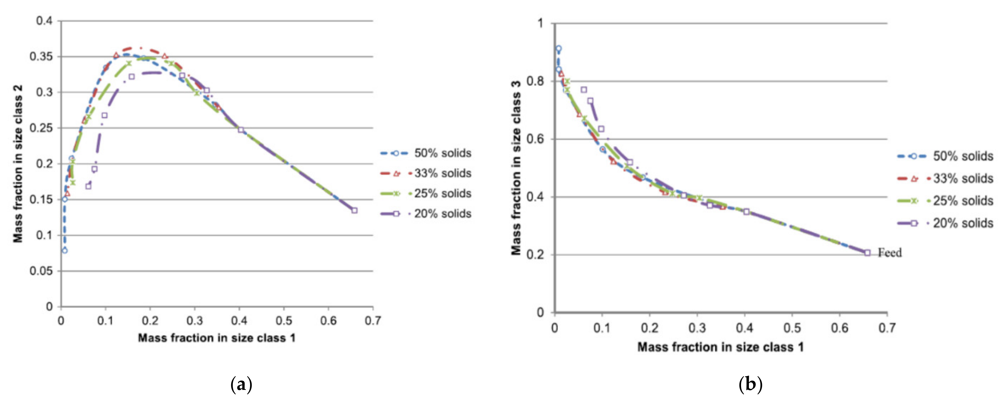
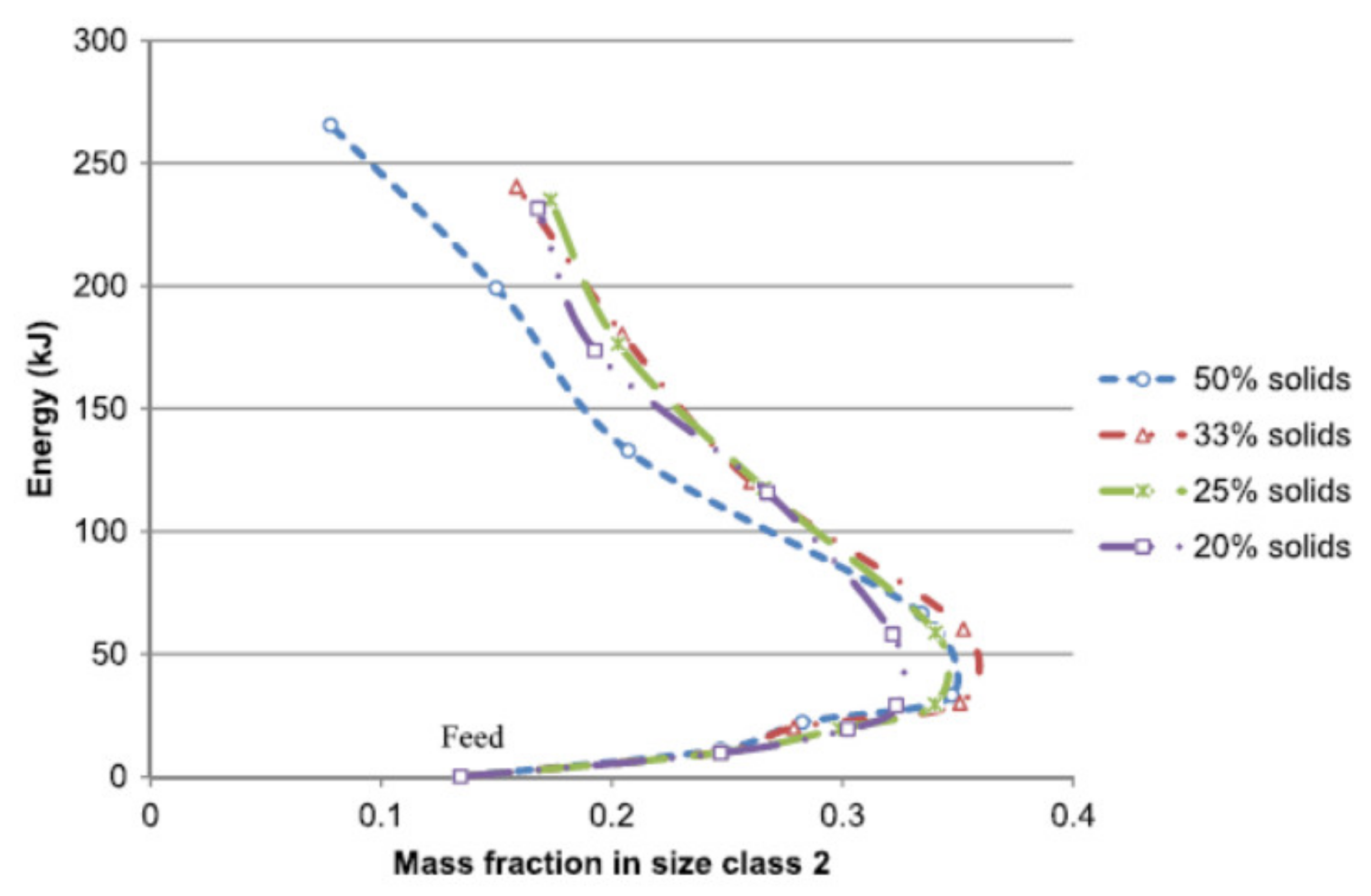
Danha et al. [51] used the AR technique to assess the optimal slurry density needed to maximise the production of the desired size fraction (−45 + 15 µm). The authors specifically used the technique to reduce the grinding period and grinding energy required to achieve their objective function. From their analysis, it was shown that within the first 10 min of grinding, the grinding rate was independent of the percent solid concentration. Further analysis of the results revealed that the 33% solid concentration produced the highest amount of m₂ within the shortest period whilst the 50% solid concentration produced the highest amount m₃ (<9 µm) as presented in Figure 12.

Even when assessed in terms of energy, the 33% solid concentration led to the most efficient use of energy to produce m₂ as depicted in Figure 13 whereas, for m₃, it was the 50% solid concentration. This demonstrates that energy expenditure is the function of slurry density which in turn is dictated by the objective function.

4. Discussion and the Future of AR in Comminution

Since its inception, the AR analytical tool has demonstrated its ability to optimise milling circuits. The work done so far has been to a greater extent on ball mill operational parameters. This is probably because ball mills are known to be the largest consumers of energy in the mining industry. Thus, most of the work undertaken so far using the novel optimisation technique has demonstrated the technique’s ability to optimise the size reduction machine. The ball mill was optimised based on the operational parameters involving the fractional ball filling (J), the fraction of critical speed (ϕ_c), powder filling (U), solids concentration, ball diameter (d) ball and feed size distributions, to achieve a given objective function which could be to maximise the production of the desired size fraction that is m₂ in some cases or m₃ in other cases. Other parameters such as the drop weight and height from the drop weight data were also optimised.

These operating parameters are complex and interactive. Thus, a graphical approach such as AR can help to visualise all possible solutions more easily for a system analysing the effect of either a single or multi-parameter on the achievement of the objective function. In a multi-parameter regime, where all parameters were varied to achieve given targets, the AR graphically showed the value of each varied parameter needed to achieve the target [19] whilst in the event where one parameter was varied whilst the others were held constant (most cases), the AR revealed the optimum value of that parameter at which the system target was achieved.

The analytical tool has provided an alternative approach of how to arrive at a product size distribution that can be optimally controlled to maximise the production of the desired size fraction. Work done on AR has established good ground for the development of the novel technique in the minerals industry. When tested at an industrial scale on a preselected industrial mill to optimize the product size distribution, its capacity to predict changes and ascertain optimal mill operating conditions was demonstrated. In some cases, the AR analysis revealed optimal conditions which have often come into conflict with some of the traditionally acceptable milling conditions under which most concentrators are operated. The conflict was in some cases attributed to the oversimplification of the processes analysed since the main objectives pursued in such work [8,13] was to demonstrate the ability of the tool to optimise processes. Thus, its application has not been adopted in the mining industry because of the conservative nature of the industry. However, the benefits availed by the AR analysis are difficult to ignore.

When applied to assess the optimal ball filling needed to produce the desired product in different research works, the AR technique pointed to different values of J needed to achieve the objective function. The analysis from laboratory data pointed to low values of J especially those of Hlabangana et al. [13] and Metzger et al. [8]. In both works, the range of ball fillings investigated was also on the low side with that of Hlabangana et al. [13] ranging from 0.3%–10.7% whilst that of Metzger et al. [8] ranging from 1.5%–21.5%. Although the ability of AR to determine optimal policies and reduce processing times and energy expenditure in ball mills and milling circuits was, in general, superbly demonstrated in these research works, there was no common platform to compare their findings with those from traditionally acceptable milling practice. Thus, Metzger et al. [8] carried out experiments at ϕ_c = 0.71 and J = 31.5% to bring the comparison closer to home. They still found that low values of J produced more of the desired size fraction than what was produced at higher values of J. The conflict in the findings among others such as oversimplified processes was attributed to the difference in the main objective functions being pursued, with that of AR being to maximise the production of the desired size fraction whilst that in traditional practices being to optimise power consumption. The other reason could also be that the effect of other operational parameters was not considered in the AR analysis, since we have learnt in the foregoing that all the parameters are complex and interactive. The powder filling was not given in the work, which also influences the particle composition of the product size distribution.

The AR analysis was then applied on scaled-up data, [10,17,19,20,23] and the results produced the values of J ranging from 35%–45% from different applications, confirming the traditionally accepted milling practices [18,33,34]. From the scaled-up data, the values of ball filling found from different AR analyses were differentiated by the transport models used as well as the objective functions. The optimisation paradigm in Chimwani et al. [23] was focused more on the trade-off between the energy and the amount of the desired size fraction produced. Although the milling operational conditions differentiated the observed ball filling values needed to produce the desired size fraction between the laboratory and full-scale milling, the ability of the AR analysis technique to condense the results into a graphical overview that is practical and easier to interpret was demonstrated.

The AR analysis of the effect of the ball mill rotational speed on a laboratory scale revealed that low speed (ϕ_c = 3%) is desirable to achieve the maximum production of the desired size, albeit with the longest grinding period [8]. The difference between the critical speed proposed by Metzger et al. [8] and those used in traditional milling practices is owing to, among other factors, the range of critical speed investigated by Metzger et al. [8] which is more on the lower side (3% to 37%), low value of J used and their objective function which was to maximise the desired size fraction with minimal energy usage. Although the objective function was achieved, the mining industry will find it difficult to use such a rotational speed owing to the longer processing time required to achieve it.

The extension of an AR analysis of the operational parameter to an industrial mill showed that the rotation rate of ϕ_c = 40% optimised the production of the desired size fraction [17,19,20,23] both in terms of the grinding time and energy. This does not agree with the common practice which recommends 75% of critical speed as optimal. Again, this is due to different objective functions pursued. Thus, it will be interesting to conduct a comprehensive cost and benefit analysis which is all-encompassing to determine the best practice since low rotational speeds have often been associated with high wear rates of mill shell liners. At present, mills are generally run at 69% of critical speed to conserve liners. Therefore, an approach that integrates all the relevant aspects of milling operations or a pilot plant needs to be developed to generate data that will provide a more authoritative set of operational parameters. Although the AR analysis has tipped the mill rotational speed to be the major player in the optimisation of milling circuits, the parameter is normally optimized at the point of plant installation.

From different investigations of the effect of powder filling undertaken, the research which involved the use of AR analysis [15,19,40] unanimously agreed that the ball mill was optimised at U = 1. This confirmed the traditionally acceptable milling practices which were influenced by previous research, preceding the dawn of AR. However, Halabangana et al. [40] argued that U is influenced by the product requirements after finding the value of U = 1.75 optimising the production of a product coarser than what was produced in other cases where the value of U = 1. Although their claim is valid, it is not surprising especially considering that as we go further upstream in terms of the product size requirements, the feed size also becomes coarser, resulting in the change of the operational conditions as influenced by other operational parameters in a dynamic system.

The ball diameter has received considerable attention from researchers. Traditionally, it is known that smaller balls grind fine particles more effectively whilst coarser particles are ground more efficiently by bigger balls [18,41,42,43,44]. Katubilwa et al. [9] confirmed that information when they found that smaller balls effectively produced materials under 75 μm. Important insights brought to light by the AR analysis are that the optimisation of other parameters such as the residence time [20], the feed size [15] and the product size distribution [17] also depend on ball size distribution. Although most of the AR work undertaken on an industrial ball mill pointed to 40 mm diameter balls as the optimum ball size to produce the desired size fraction, it is important to note that the optimisation scheme was performed using mono size balls. Therefore, it is reiterated that a mixture of balls would perform better than any mono size to grind a feed with a wider particle size distribution since it would take advantage of both small and large media and that reinforces what is conventionally known about the subject [10]. What is still sparse though in the literature is the optimisation of the ratio of ball sizes against the feed size distribution. Since the feed size distribution from a continuous feed is dynamic, so should be the ball size distribution. However, matching such a dynamic process would be difficult, which then brings to light the need for mills in series with each mill, grinding tailored feed using ball sizes optimised for that particular mill. This can be achieved using the methodology used by Chimwani et al. [22] in which the authors investigated the make-up ball charge using AR analysis that enables the achievement of the objective function since it aligns with the practical approach practised in industry.

The AR analysis from drop weight test data conducted revealed that large ball sizes were desired for producing m₃ [12] since they promote the breakage of most of the material from m₁ to m₃. Although it is true for drop weight set up, the opposite is true in an industrial ball mill as confirmed by AR and non-AR analysis results. This is possibly due to the different orientation of balls between the drop-weight test and ball mill set up, which are well-defined and stochastically varying, respectively. As for the ball shape, the AR analysis by Hlabangana et al. [16] revealed that the ellipsoid produced the highest amount of m₂ whilst that of Emmanuel et al. [25] suggested the sphere-shaped balls as the desired balls for maximising the production of m₃. This consolidates the assertion that product requirements are also a function of ball shapes in a grinding environment.

The AR analysis work conducted to optimise feed size distribution by a couple of researchers led them to converge on a conclusion that a feed size distribution is efficiently ground by a mixture of ball sizes. This agrees with a widely known fact that small particles are effectively ground by small balls and so are the bigger particles by bigger balls [15,24]. Although the subject has not received wide coverage, the conclusion from the few pieces of research undertaken, which recommends close monitoring of the match between the feed size and ball size distribution, is noteworthy. Feed tailoring has also come in handy in ensuring optimisation of the ball mill from the feed size distribution perspective since it promotes the matching of the ball size distribution with the particles being fed into the mill. Small ball mills in series which offer smaller residence time to particles as proposed by Chimwani et al. [24] reinforce the feed tailoring technique. This is true especially considering that feed tailoring can be valuable in ball milling only up to a certain operation time, beyond which the nature of the feed distribution ceases to be of significance to the performance of the mill.

The solid content has also not received much attention as far as AR analysis is concerned, which makes it a fertile field of research. The only research conducted using the novel technique suggested different solid concentrations for different objective functions [11]. Lower values (33%) were proposed [11] than what is currently used in industry (40%–45%) from earlier research [49,50]. The disparity between the values proposed requires further investigations to be conducted on a pilot scale in a continuous milling environment using the AR analysis.

The comprehensive assessment of the cost and benefit analysis of the settings proposed by the AR on a pilot plant would determine whether the technique will be adopted or not. Especially considering that no company would want to stop a fully operational plant to test the recommendations from AR analysis at the expense of production output.

Summary

The AR has shown great potential to optimise milling circuits. For systems investigated, the novel technique not only enabled the determination of performance targets but also the configuration of mills to achieve the set targets and objective functions. What differentiates the AR analysis results from different operational scales is the difference in operational conditions emanating from the complex and interactive nature of the operating parameters. Ranges of values investigated which did not cover the whole spectrum of possible values also contributed to the differences observed in some instances between what is conventionally known, and the AR analysis results. The other contributing factor was the optimisation approach, which in some cases focused on all operational parameters at once whilst in some other cases which comprise the majority; the parameters were optimised one at a given time. The objective functions defined by the process targets also contributed to what differentiates the AR results from the conventional milling practices currently followed in the industry. The other notable factor that also contributed to the disparity is the oversimplification of the processes analysed which needed to underscore the underlying concepts and principles of application of the AR tool in milling processes optimisation. Nonetheless, the opportunities offered by the AR technique are overwhelming hence difficult to ignore. Therefore, to encourage its adoption in the industry, the next stage is to apply it to a pilot plant that mimics a real mineral processing plant.

5. Conclusions

This review has shown important milestones reached by the AR methodology in the optimisation of ball milling circuits. The AR analysis has demonstratively produced the process targets and the control policies to achieve the targets of different operational parameters. When analysed at different operational scales i.e., laboratory batch scale and full-scale continuous milling:

• Low values of J produced more of the desired size fraction than higher values of J at the laboratory scale showing the disparity between the AR results and what is conventionally known in the mining industry. The difference was largely owing to different main objective functions being pursued.
• J values optimised using AR analysis from the industrial and continuous milling data range from 35%–45% for different applications, confirming the traditionally accepted milling practices in the mining industry.
• Low speeds are desirable for the maximum production of the desired size fraction, at the laboratory scale as per the AR analysis.
• At an industrial scale, ϕ_c = 40% optimised the production of the desired size fraction in terms of energy, disagreeing with 75% currently used in industry. The objective functions pursued contribute to this difference as well.
• There is unanimous agreement in literature both from traditional practices and AR point of view that the ball mill is optimised at U = 1.
• Optimisation of other parameters such as the residence time, the feed size and the product size distribution also depend on ball size distribution.
• What is common across all the optimisation techniques regardless of the objective function is that a mixture of balls efficiently breaks a wide feed size distribution since it takes advantage of both small and large media and that it reinforces what is conventionally known about the subject.
• Feed tailoring promotes the matching of the ball size distribution with the particles being fed into the mill.
• Small ball mills in series which offer smaller residence time to particles are suitable for tailored feeds since the difference in feed size distribution ceases to be significant beyond a certain operating time.
• The optimum slurry density from an AR analysis point of view is lower than what is currently used in the industry.

The opportunities offered by the AR technique are noteworthy and hence are difficult to overlook. Therefore, to encourage its adoption in the industry, the next stage is to apply it to a pilot plant that mimics a real mineral processing plant. Thorough investigations of the solids concentration in slurry, the feed flow rate and the ball size distribution are needed from an AR perspective. Then, the study of milling circuit configurations can be integrated in order to consolidate the position of the AR technique as an alternative analysis tool.