Development of a Higher-Order 𝒜-Stable Block Approach with Symmetric Hybrid Points and an Adaptive Step-Size Strategy for Integrating Differential Systems Efficiently

Abstract

This article introduces a computational hybrid one-step technique designed for solving initial value differential systems of a first order, which utilizes second derivative function evaluations. The method incorporates three intra-step symmetric points that are calculated to provide an optimum version of the suggested scheme. By combining the hybrid and block methodologies, an efficient numerical method is achieved. The hybrid nature of the algorithm determines that the first Dahlquist barrier is overcome, ensuring its effectiveness. The proposed technique exhibits an eighth order of convergence and demonstrates $\mathcal{A}$-stability characteristics, making it particularly well suited for handling stiff problems. Additionally, an adjustable step size variant of the algorithm is developed using an embedded-type technique. Through numerical experiments, it is shown that the suggested approach outperforms some other well-known methods with similar properties when applied to initial-value ordinary differential problems.

1. Introduction

In this article, our aim is to construct an efficient algorithm for integrating initial-value differential problems given by

$${\mathbf{z}}^{\prime }\left(x\right)=\mathbf{f}(x,\mathbf{z});\mathbf{z}\left(x_0\right)={\mathbf{z}}_{\mathbf{0}},$$

(1)

with $x\in [x_0,x_N],\mathbf{z}:[x_0,x_N]\to {\mathbb{R}}^m,\mathbf{f}:[x_0,x_N]\times {\mathbb{R}}^m\to {\mathbb{R}}^m$, assuming that all prerequisites for the existence of a unique solution are fulfilled.

Differential equations are used to model continuous phenomena that frequently occur in real-world situations. Unfortunately, very few of such equations can be tackled analytically. In this scenario, usually the problem of interest is dealt with numerically, that is, an approximate solution is obtained on a discrete set of points. The classes of Runge–Kutta and linear multi-steps techniques have usually been to obtain reliable approximations of the true solution of (1). For more details, one can see the monographs written by Butcher [1], Hairer [2,3], Lambert [4], Brugnano [5], Rosser [6] and Milne [7]. In Matlab and Mathematica, many ODE solvers are incorporated with the purpose of carrying out the task efficiently. For a detailed description of the codes, one can see the references by Shampine et al. [8,9] and Dormand and Prince [10]. Some of these built-in codes are specifically designed for solving stiff and non-stiff systems, for instance, the ODE23s solver is an integrated function explicitly crafted to manage stiff systems, as noted by Shampine et al. [11]. It excels particularly when dealing with coarse tolerances. This solver relies on an adapted Rosenbrock approach of a second order, employing a variable step size methodology through a blend of precise second and third-order formulas, effectively estimating the solution. The development of efficient algorithms with good stability characteristics is a major problem of interest in the numerical analysis of differential systems.

The first Dahlquist’s barrier, as is well known, limits the order that can be achieved in the class of zero-stable linear multi-step methods. Dahlquist established that the order of accuracy, say p, of a linear m-step method is as follows:

$$\left\{\begin{array}{c}p\le m+1,\mathrm{when}m\mathrm{is}\mathrm{odd},\hfill \\ p\le m+2,\mathrm{when}m\mathrm{is}\mathrm{even}.\hfill \end{array}\right.$$

To overcome the limitations of linear multi-step methods, numerous researchers have proposed hybrid approaches which include information from the solution at off-step points within the required interval of interest. These hybrid methods have also been referred to as linear multi-step methods of a modified type [1]. For a more comprehensive understanding of these techniques, Lambert’s book [4] serves as a valuable resource. Block methods were initially designed to obtain starting guesses for implicit multi-step methods, but they have evolved to be used in general-purpose codes [12]. These block methods aim to provide the approximate solution at various grid points at once (see [13]). For an extensive list of references on these methods, interested readers may refer to Lambert’s book and Brugnano’s work [4,5].

Here, we have used both approaches, namely hybrid and block, to develop a new method using interpolation and collocation techniques. An optimized version of the method can be obtained by following an appropriate optimization strategy. The obtained algorithm can be considered an extended version of the one presented in [14]. Additionally, the technique is devised in an adaptive step size version, employing an embedded-type technique.

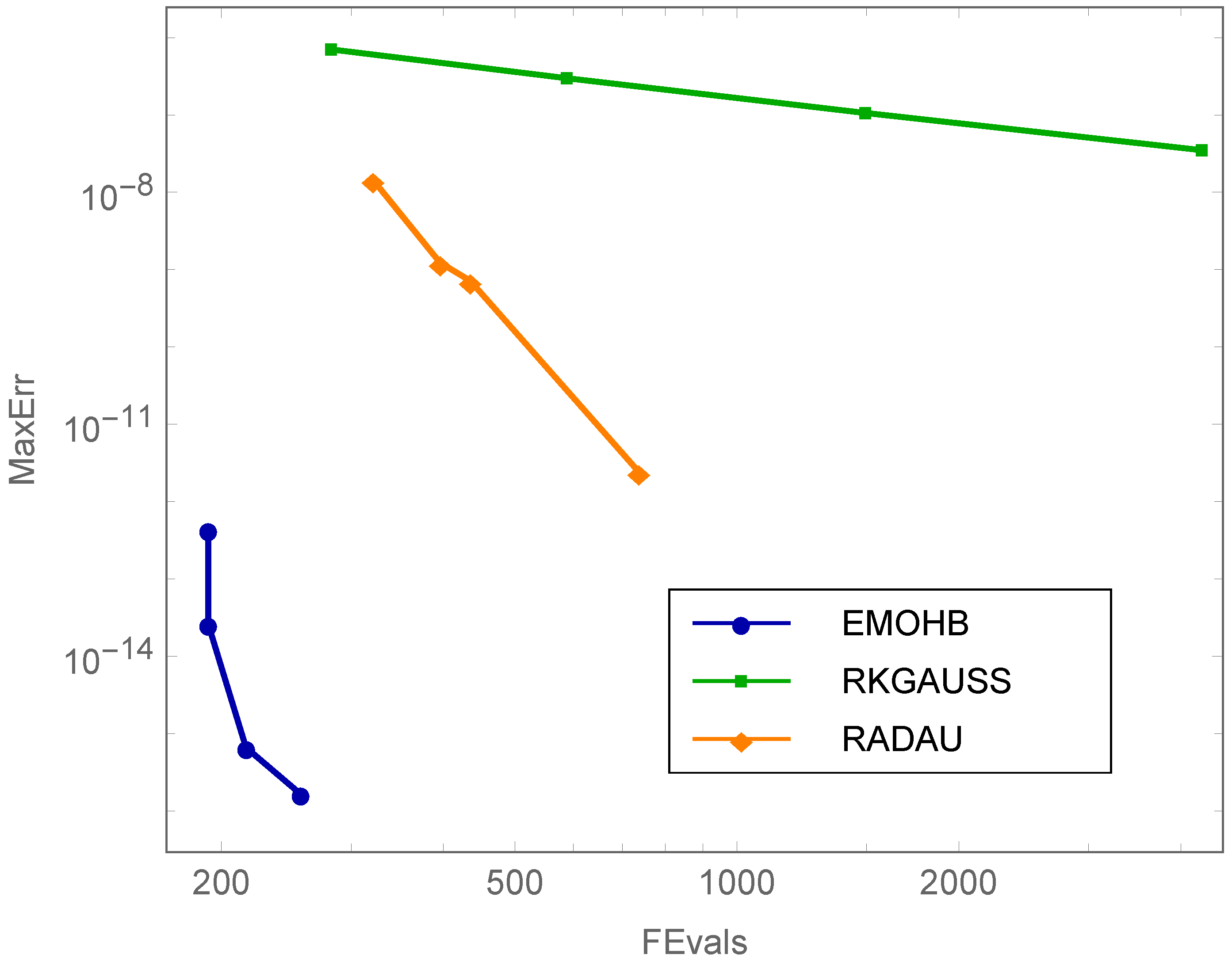
The article’s content is organized into the following sections: Section 2 contains the derivation of the new algorithm. In Section 3, the primary characteristics of the proposed method are examined. The formulation of the new method in adaptive step size mode is elaborated on in Section 4. 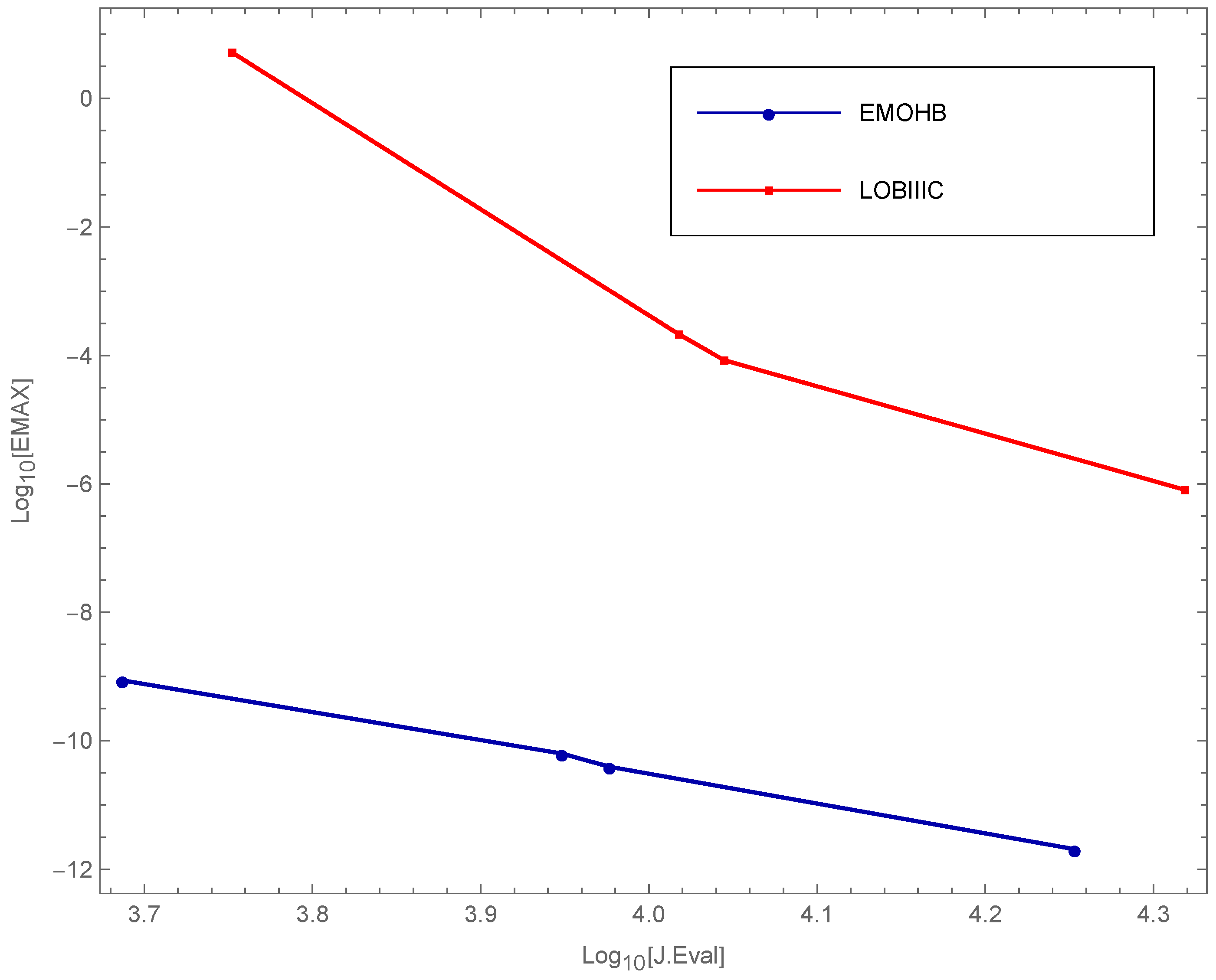The performance of the proposed method, compared to some existing methods in the literature, is demonstrated through numerical experiments in Section 5. In Section 6, the efficiency curves have been plotted, which reflects the better performance of the proposed scheme. Finally, Section 7 shows some conclusions drawn from the study.

2. Construction of the Proposed Scheme

For the sake of simplicity, the method is derived for solving the differential system (1) with $m=1$, and then, by using the component-wise strategy it could be applied for solving problems with $m>1$. Let us consider a fixed step size $h=x_{j+1}-x_j$ on a discrete grid with $N+1$ points, $x_0<x_1<\cdots <x_N$. To derive the method, begin by considering the theoretical solution of (1) in the form of an interpolating polynomial expressed as:

$$z\left(x\right)\approx R\left(x\right)=\sum _{i=0}^{{\eta }_1+{\eta }_2-1}{\mathrm{\Psi }}_i{\mathrm{\Theta }}_i\left(x\right),x\in [x_j,x_{j+k}].$$

(2)

Consider ${\eta }_1$ as the numbers of interpolation points and ${\eta }_2$ as that of collocation points, satisfying $0\le {\eta }_1\le k$ and ${\eta }_2>0$, with k denoting the number of steps in the block, with $k>0$. The terms ${\mathrm{\Psi }}_i$ are unknown constants to be calculated, and ${\mathrm{\Theta }}_i\left(x\right)={(x-x_j)}^i$ represents the polynomial basis functions. To introduce a hybrid nature to the proposed method, three values, $r_1,r_2=1/2$, and $r_3\in [0,1]$, are chosen such that $x_{j+r_1}=x_j+r_1·h$, $x_{j+r_2}=x_j+r_2·h$, and $x_{j+r_3}=x_j+r_3·h$ represent three intra-step points. The development of the present method involves specifying the parameters ${\eta }_1=1$, ${\eta }_2=8$, and $k=1$. The derivation of the method is detailed below:

Step 1: 

The unknown coefficients ${\mathrm{\Psi }}_i$ in (2) are determined by imposing the following conditions:

(i)

$z\left(x_j\right)=R\left(x_j\right)$

(ii)

$z^{\prime }\left(x_{j+v}\right)=R^{\prime }\left(x_{j+v}\right),v=0,r_1,r_2,r_3,1$

(iii)

$z^{″}\left(x_{j+v}\right)=R^{″}\left(x_{j+v}\right),v=0,r_2,1$

Hence, a system of nine equations in nine unknowns ${\mathrm{\Psi }}_i,i=0\left(1\right)8$ is obtained. This system can be solved by using a computer algebra system (CAS). After substituting the obtained ${\mathrm{\Psi }}_i^{\prime }s$ into (2), we get

$$z\left(x\right)\approx R\left(x\right)=\lambda \left(x\right)z_j+h\left(\sum _{i=0}^1{\mu }_i\left(x\right)f_{j+i}+\sum _{i=1}^3{\mu }_{r_i}\left(x\right)f_{j+r_i}\right)+h^2\left({\sigma }_0\left(x\right)f_j^{\prime }+{\sigma }_{r_2}\left(x\right)f_{j+r_2}^{\prime }+{\sigma }_1\left(x\right)f_{j+1}^{\prime }\right)$$

(3)

where

$$\begin{array}{ccc}\hfill f_{j+m}& =& f(x_{j+m},z_{j+m}),m=0,r_1,r_2,r_3,1,\hfill \\ \hfill f_{j+m}^{\prime }& =& f^{\prime }(x_{j+m},z_{j+m}),m=0,r_2,1\mathrm{and}{z}_{j+m}\simeq z\left(x_{j+m}\right).\hfill \end{array}$$

Step 2: 

In order to obtain optimized values for $r_1$ and $r_3$, we evaluate expression (3) at $x=x_{j+1}$ and $x=x_{j+r_2}$. This allows us to approximate the true solution at the final point and at the midpoint of the interval $[x_j,x_{j+1}]$, denoted as $x_{j+1}$ and $x_{j+r_2}$, respectively, in terms of $r_1$ and $r_3$, as shown in [15]. The evaluation of $z\left(x_{j+1}\right)$ and $z\left(x_{j+r_2}\right)$ can be readily obtained through a CAS, although the resulting expressions can be quite lengthy, and so they are not presented here. To determine the appropriate values of the unknown parameters $r_1$ and $r_3$, the following optimization strategy is employed:

(i)

By expanding the formulas for $z\left(x_{j+1}\right)$ and $z\left(x_{j+r_2}\right)$ using the Taylor series around $x_j$, we obtain the local truncation errors of these formulas, which are given by

$$\mathcal{L}(z\left(x_{j+1}\right),h)={\displaystyle \frac{(-2+r_1(3-6r_3)+3r_3)z^{\left(9\right)}\left(x_j\right)h^9}{203,212,800}}+\mathcal{O}\left(h^{10}\right)$$

(4)

and

$$\mathcal{L}(z\left(x_{j+r_2}\right),h)={\displaystyle \frac{(-23+r_1(87-384r_3)+87r_3)z^{\left(9\right)}\left(x_j\right)h^9}{26,011,238,400}}+\mathcal{O}\left(h^{10}\right).$$

(5)

(ii)

By setting the leading terms of the truncation errors in (4) and (5) equal to zero, we arrive at the following system of nonlinear equations:

$$\left\{\begin{array}{cc}-2+r_1(3-6r_3)+3r_3\hfill & =0\hfill \\ -23+r_1(87-384r_3)+87r_3\hfill & =0.\hfill \end{array}\right.$$

(iii)

The implicit system of equations above represents two curves in the $r_1{r}_3$-plane, exhibiting symmetry with respect to the diagonal $r_1=r_3$. A unique solution satisfying the condition $0<r_1<r_2<r_3<1$ is obtained, and it is given by:

$$r_1={\displaystyle \frac{1}{6}}\left(3-\sqrt{3}\right)\simeq 0.211325,r_3={\displaystyle \frac{1}{6}}\left(3+\sqrt{3}\right)\simeq 0.788675.$$

Substituting the optimal values of $r_1$ and $r_3$ in the expressions (4) and (5), we get

$$\mathcal{L}(z\left(x_{j+1}\right),h)=-{\displaystyle \frac{z^{\left(11\right)}\left(x_j\right)h^{11}}{1,207,084,032,000}}+\mathcal{O}\left(h^{12}\right),$$

(6)

$$\mathcal{L}(z\left(x_{j+r_2}\right),h)={\displaystyle \frac{z^{\left(10\right)}\left(x_j\right)h^{10}}{133,772,083,200}}+\mathcal{O}\left(h^{11}\right).$$

(7)

Note that using the optimized values of $r_1$ and $r_3$, we gain at least an order of accuracy in the formulas to approximate $z_{j+1}$ and $z_{j+r_2}$.

Step 3: 

Finally, we require approximations of the true solution at the remaining intra-step points, that is, at $x=x_{j+r_1},x_{j+r_3}$. These are obtained by substituting the optimized values of $r_1,r_3$ and $x=x_j+r_{1}h,x_j+r_{3}h$ in the expression in (3). The proposed hybrid method provides four approximations of the true solution at $x_{j+r_1},x_{j+r_2},x_{j+r_3},x_{j+1}$. The coefficients of each of the formulas of the block method are listed in

Table 1. Coefficients of the method.

z	$\lambda$	${\mu }_0$	${\mu }_{r_1}$	${\mu }_{r_2}$	${\mu }_{r_3}$	${\mu }_1$	${\sigma }_0$	${\sigma }_{r_2}$	${\sigma }_1$
$z_{j+r_1}$	1	$\frac{727+44\sqrt{3}}{7560}$	$\frac{\left(108+\sqrt{3}\right)}{840}$	$-\frac{4\left(-36+23\sqrt{3}\right)}{945}$	$\frac{\left(36-23\sqrt{3}\right)}{280}$	$\frac{-43+44\sqrt{3}}{7560}$	$\frac{62+9\sqrt{3}}{22,680}$	$\frac{1}{162}$	$\frac{8-9\sqrt{3}}{22,680}$
$z_{j+r_2}$	1	$\frac{619}{6720}$	$\frac{9}{70}+\frac{9\sqrt{3}}{128}$	$\frac{16}{105}$	$\frac{9}{70}-\frac{9\sqrt{3}}{128}$	$-\frac{11}{6720}$	$\frac{67}{26,880}$	$-\frac{1}{96}$	$\frac{1}{8960}$
$z_{j+r_3}$	1	$\frac{727-44\sqrt{3}}{7560}$	$\frac{\left(36+23\sqrt{3}\right)}{280}$	$\frac{4\left(36+23\sqrt{3}\right)}{945}$	$\frac{\left(108-\sqrt{3}\right)}{840}$	$\frac{-43-44\sqrt{3}}{7560}$	$\frac{62-9\sqrt{3}}{22,680}$	$\frac{1}{162}$	$\frac{8+9\sqrt{3}}{22,680}$
$z_{j+1}$	1	$\frac{19}{210}$	$\frac{9}{35}$	$\frac{32}{105}$	$\frac{9}{35}$	$\frac{19}{210}$	$\frac{1}{420}$	0	$-\frac{1}{420}$

.

This proposed method is implicit in nature, requiring the solution of a system of four equations at each iteration. The commonly employed approach to solve this system is Newton’s method or its variants, as outlined in [12].

3. Method Analysis: Examining Its Characteristics

Now, we discuss some basic characteristics of the method presented in Table 1, as the order of accuracy, zero-stability, and the analysis of linear stability.

3.1. Order of Accuracy and Consistency

To address the convergence analysis, we rewrite the method whose coefficients are given in Table 1 as

$$A{\mathbf{Z}}_J=hB{\mathbf{F}}_J+h^{2}C{\mathbf{G}}_J,$$

(8)

where $A,B$, and C are matrices of dimension $4\times 5$, given by

$$A=\left(\begin{array}{ccccc}-1& 1& 0& 0& 0\\ -1& 0& 1& 0& 0\\ -1& 0& 0& 1& 0\\ -1& 0& 0& 0& 1\end{array}\right),$$

$$B=\left(\begin{array}{ccccc}\frac{727+44\sqrt{3}}{7560}& \frac{\left(108+\sqrt{3}\right)}{840}& -\frac{4\left(-36+23\sqrt{3}\right)}{945}& \frac{\left(36-23\sqrt{3}\right)}{280}& \frac{-43+44\sqrt{3}}{7560}\\ \frac{619}{6720}& \left(\frac{9}{70}+\frac{9\sqrt{3}}{128}\right)& \frac{16}{105}& \left(\frac{9}{70}-\frac{9\sqrt{3}}{128}\right)& -\frac{11}{6720}\\ \frac{727-44\sqrt{3}}{7560}& \frac{\left(36+23\sqrt{3}\right)}{280}& \frac{4\left(36+23\sqrt{3}\right)}{945}& \frac{\left(108-\sqrt{3}\right)}{840}& \frac{-43-44\sqrt{3}}{7560}\\ \frac{19}{210}& \frac{9}{35}& \frac{32}{105}& \frac{9}{35}& \frac{19}{210}\end{array}\right),$$

$$C=\left(\begin{array}{ccccc}\frac{62+9\sqrt{3}}{22,680}& 0& \frac{1}{162}& 0& \frac{8-9\sqrt{3}}{22,680}\\ \frac{67}{26,880}& 0& -\frac{1}{96}& 0& \frac{1}{8960}\\ \frac{62-9\sqrt{3}}{22,680}& 0& \frac{1}{162}& 0& \frac{8+9\sqrt{3}}{22,680}\\ \frac{1}{420}& 0& 0& 0& -\frac{1}{420}\end{array}\right)$$

and

$$\begin{array}{cc}\hfill {\mathbf{Z}}_{\mathbf{J}}& ={(z_j,z_{j+r_1},z_{j+r_2},z_{j+r_3},z_{j+1})}^T,\hfill \\ \hfill {\mathbf{F}}_{\mathbf{J}}& ={(f_j,f_{j+r_1},f_{j+r_2},f_{j+r_3},f_{j+1})}^T,\hfill \\ \hfill {\mathbf{G}}_{\mathbf{J}}& ={(f_j^{\prime },f_{j+r_1}^{\prime },f_{j+r_2}^{\prime },f_{j+r_3}^{\prime },f_{j+1}^{\prime })}^T.\hfill \end{array}$$

The linear difference operator $\overline{\mathbb{L}}$ related to the difference block given in (8) can be expressed as follows:

$$\overline{\mathbb{L}}[z\left(x\right),h]=\sum _j{\overline{\rho }}_{j}z(x+jh)-h\sum _j{\overline{\delta }}_j{z}^{\prime }(x+jh)-h^2\sum _j{\overline{\gamma }}_j{z}^{″}(x+jh),j=0,r_1,r_2,r_3,1$$

(9)

where ${\overline{\rho }}_j,{\overline{\delta }}_j$, and ${\overline{\gamma }}_j$ are precisely the column vectors of matrices $A,B$ and C. We make the assumption that $z\left(x\right)$ is sufficiently differentiable to expand $z(x+jh)$, $z^{\prime }(x+jh)$, and $z^{″}(x+jh)$ in Taylor series around x. In this way we get

$$\overline{\mathbb{L}}[z\left(x\right),h]={\overline{\tau }}_{0}z\left(x\right)+{\overline{\tau }}_{1}h{z}^{\prime }\left(x\right)+{\overline{\tau }}_2{h}^2{z}^{″}\left(x\right)+\cdots +{\overline{\tau }}_p{h}^p{z}^{\left(p\right)}\left(x\right)+\cdots$$

(10)

Definition 1.

The linear operator in (9) and the method whose coefficients are given in Table 1 are regarded as being of order p when the condition stated in (10) produces

$${\overline{\tau }}_0={\overline{\tau }}_1={\overline{\tau }}_2=\cdots ={\overline{\tau }}_p=\mathbf{0}\mathrm{and}{\overline{\tau }}_{p+1}\ne \mathbf{0}.$$

We note that the ${\overline{\tau }}_i^{\prime }s$ are vectors and ${\overline{\tau }}_{p+1}$ is known as the vector of error constants, being

$$\overline{\mathbb{L}}[z\left(x\right),h]=-{\overline{\tau }}_{p+1}{h}^{p+1}{z}^{(p+1)}\left(x\right)+\mathcal{O}\left(h^{p+2}\right).$$

Concerning the obtained method, it is ${\overline{\tau }}_0={\overline{\tau }}_1={\overline{\tau }}_2=\cdots ={\overline{\tau }}_8=\mathbf{0}$ and

$${\overline{\tau }}_9={\left(-{\displaystyle \frac{1}{1,881,169,920\sqrt{3}}},0,{\displaystyle \frac{1}{1,881,169,920\sqrt{3}}},0\right)}^T$$

with

$$\overline{\mathbb{L}}[z\left(x\right),h]=\left(\begin{array}{c}-\frac{1}{1,881,169,920\sqrt{3}}{h}^9{z}^9\left(x\right)+\mathcal{O}\left(h^{10}\right)\\ \frac{1}{133,772,083,200}{h}^{10}{z}^{10}\left(x\right)+\mathcal{O}\left(h^{11}\right)\\ \frac{1}{1,881,169,920\sqrt{3}}{h}^9{z}^9\left(x\right)+\mathcal{O}\left(h^{10}\right)\\ -\frac{1}{1,207,084,032,000}{h}^{11}{z}^{11}\left(x\right)+\mathcal{O}\left(h^{12}\right)\end{array}\right).$$

This indicates that the proposed method in Table 1 has order $p=8$. Since $p\ge 1$, this characteristic serves as a sufficient condition for ensuring the consistency of the corresponding block method.

3.2. Zero-Stability Analysis

The primary focus of this subsection lies in analyzing the stability of the difference Equation (8) when h tends to zero. In this case, the method in Table 1 reduces to $z_{j+r_1}=z_j,z_{j+r_2}=z_j,z_{j+r_3}=z_j,z_{j+1}=z_j$, which can further be rewritten in a more convenient way as

$${\widehat{W}}_{\zeta }=\overline{A}{\widehat{W}}_{\zeta -1},$$

(11)

where

$$\overline{A}=\left(\begin{array}{cccc}0& 0& 0& 1\\ 0& 0& 0& 1\\ 0& 0& 0& 1\\ 0& 0& 0& 1\end{array}\right)$$

and

$$\begin{array}{cc}\hfill {\widehat{W}}_{\zeta }& ={(z_{j+r_1},z_{j+r_2},z_{j+r_3},z_{j+1})}^T,\hfill \\ \hfill {\widehat{W}}_{\zeta -1}& ={(z_{j+r_1-1},z_{j+r_2-1},z_{j+r_3-1},z_j)}^T.\hfill \end{array}$$

(12)

The first characteristic polynomial of the proposed block method is

$$\rho \left(\eta \right)=det[I_4\eta -\overline{A}]={\eta }^3(\eta -1).$$

(13)

Since the roots of the equation $\rho \left(\eta \right)=0$ fulfill ${\eta }_j\le 1$, and the root with a modulus of one is simple, the proposed method is considered to be zero-stable according to [2].

3.3. Convergence

As per the Lax equivalence theorem, a method is deemed to be convergent if and only if it satisfies both consistency and zero-stability. In the preceding sections, we have demonstrated the consistency and zero-stability of the newly developed method, leading to the conclusion that the method presented in Table 1 is convergent.

3.4. Linear Stability Analysis

The notion of linear stability differs from zero stability since zero stability analysis involves considering the step size $h\to 0$. In practical applications, we always work with finite step sizes, i.e., $h>0$.

Let us consider the well-known Dahlquist’s test equation:

$$z^{\prime }\left(x\right)=\gamma z\left(x\right),Re\left(\gamma \right)<0.$$

(14)

The theoretical solution to this problem is represented by $z\left(x\right)=e^{\gamma x}$, exhibiting a tendency to approach zero as x approaches infinity. It is anticipated that when employing the proposed method to solve the test problem (14), the resulting numerical solution will exhibit a similar behavior to the analytical solution. To ascertain the region in which the numerical method reproduces the true behavior of the test problem’s solutions, we apply the proposed method to the problem described in (14), thereby obtaining a system of equations.

$$M{\widehat{W}}_{\zeta }=N{\widehat{W}}_{\zeta -1}$$

(15)

where

$$M=\left[\begin{array}{cc}{B}_{11}& B_{12}\\ B_{21}& B_{22}\end{array}\right]$$

with

$$B_{11}=\left(\begin{array}{cc}\frac{840-\left(108+\sqrt{3}\right)H}{840}& \frac{\left(-864+552\sqrt{3}-35H\right)H}{5670}\\ -\frac{9\left(64+35\sqrt{3}\right)H}{4480}& 1-\frac{16H}{105}+\frac{H^2}{96}\end{array}\right),$$

$$B_{12}=\left(\begin{array}{cc}\frac{\left(-36+23\sqrt{3}\right)H}{280}& \frac{H\left(-3\left(89+\sqrt{3}\right)+\left(19+\sqrt{3}\right)H\right)}{22,680\left(1+\sqrt{3}\right)}\\ \frac{\left(-576+315\sqrt{3}\right)H}{4480}& \frac{(44-3H)H}{26,880}\end{array}\right),$$

$$B_{21}=\left(\begin{array}{cc}-\frac{\left(36+23\sqrt{3}\right)H}{280}& -\frac{H\left(864+552\sqrt{3}+35H\right)}{5670}\\ -\frac{9H}{35}& -\frac{32H}{105}\end{array}\right),$$

$$B_{22}=\left(\begin{array}{cc}\frac{840+\left(-108+\sqrt{3}\right)H}{840}& \frac{H\left(129+132\sqrt{3}-8H-9\sqrt{3}H\right)}{22,680}\\ -\frac{9H}{35}& \frac{(420+(-38+H\left)H\right)}{420}\end{array}\right)$$

and

$$N=\left(\begin{array}{cccc}0& 0& 0& \frac{22,680+H\left(2181+132\sqrt{3}+62H+9\sqrt{3}H\right)}{22,680}\\ 0& 0& 0& \frac{26,880+H(2476+67H)}{26,880}\\ 0& 0& 0& \frac{22,680+H\left(2181-132\sqrt{3}+\left(62-9\sqrt{3}\right)H\right)}{22,680}\\ 0& 0& 0& \frac{(420+H(38+H\left)\right)}{420}\end{array}\right),$$

with $H=\gamma h$ and ${\widehat{W}}_{\zeta },{\widehat{W}}_{\zeta -1}$ as in (12).

In order to understand the stability characteristics of the proposed hybrid block method, (15) is rewritten as

$${\widehat{W}}_{\zeta }=G\left(H\right){\widehat{W}}_{\zeta -1}$$

(16)

where $G\left(H\right)=M^{-1}N$ is known as the stability matrix. The stability properties of the derived method rely on evaluating the magnitude of the eigenvalues of the stability matrix, with particular emphasis on the spectral radius, denoted as $\rho \left[G\right(H\left)\right]$. The region of absolute stability, denoted as S, is defined as explained in [3].

$$S=\{H\in \mathbb{C}:|\rho \left[G\right(H\left)\right]|<1\}.$$

If the region of absolute stability contains the entire left-half complex plane, i.e., ${\mathbb{C}}^{-}\subseteq S$, then the method is considered to be $\mathcal{A}$-stable. The spectral radius of the stability matrix $G\left(H\right)$ is given by

$$\rho \left[G\left(H\right)\right]={\displaystyle \frac{R\left(H\right)}{S\left(H\right)}},$$

(17)

where

$$\begin{array}{cc}\hfill R\left(H\right)& =483,840+241,920H+55,440H^2+7560H^3+660H^4+36H^5+H^6,\hfill \\ \hfill S\left(H\right)& =483,840-241,920H+55,440H^2-7560H^3+660H^4-36H^5+H^6.\hfill \end{array}$$

The absolute value of the spectral radius given in (17) is less than unity on the left-half complex plane. This establishes the conclusion that the method whose coefficients are given in Table 1 is $\mathcal{A}$-stable. Hence, the interval of absolute stability for the proposed method is $(-\infty ,0)$.

4. Adaptive Step-Size Formulation

The proposed method (8) can be transformed into an adaptive step-size algorithm by adopting a procedure similar to the one described in [11]. This procedure involves executing two approaches of different orders, denoted as p and q, with $p>q,$ simultaneously. The combination of formulas involves using the lower-order formula to estimate the local error at each integration step, while the higher-order method advances the solution. The careful selection of this pair is crucial. To maintain the computational cost at the same level, the formula of the lower order is chosen in a manner that it does not need new function evaluations. In this way, there will be no increase in the computational cost in terms of the number of function evaluations.

The detailed procedure is as follows:

In the present case, the following implicit block formula of a lower order ($q=7$) with local truncation error $LTE=-\frac{19z^{\left(8\right)}\left(x_j\right)h^8}{304,819,200}+\mathcal{O}\left(h^9\right)$ is considered

$$z_{j+1}^{*}=z_j+h\left(\frac{19}{105}{f}_j+\frac{36-19\sqrt{3}}{140}{f}_{j+r_1}+\frac{32}{105}{f}_{j+r_2}+\frac{36+19\sqrt{3}}{140}{f}_{j+r_3}\right)+h^2\left(\frac{5}{504}{f}_j^{\prime }-\frac{19}{315}{f}_{j+r_2}^{\prime }+\frac{13}{2520}{f}_{j+1}^{\prime }\right).$$

The considered lower-order formula is firstly used to compute the approximate solution of the system at the final point of the block interval, $x_{j+1}$, denoted as $z_{j+1}^{*}$. It is worth noting that this computation will not involve any additional computational efforts concerning new function evaluations. We have established that the local error $LT{E}_1$ obtained for the approximation $z_{j+1}^{*}$ is

$$LT{E}_1=z(x_j+h)-z_{j+1}^{*}=\mathcal{O}\left(h^{q+1}\right)$$

(18)

where $z\left(x\right)$ represents the continuous solution of the problem.

Secondly, the solution of the problem is also approximated at the same block interval with the proposed higher-order block method ($p=8$) of interest. The obtained numerical solution at the final point is denoted as $z_{j+1}$ and the local error $LT{E}_2$ obtained in this case is

$$LT{E}_2=z(x_j+h)-z_{j+1}=\mathcal{O}\left(h^{p+1}\right).$$

(19)

In the next step, the unknown exact solution $z(x_j+h)$ can be eliminated by differencing Equation (18) from (19), and the obtained expression is denoted as $Eest$

$$\begin{array}{cc}\hfill Eest& =z_{j+1}-z_{j+1}^{*}=LT{E}_1+\mathcal{O}\left(h^{p+1}\right).\hfill \end{array}$$

(20)

For sufficiently small values of h, the term $\mathcal{O}\left(h^{q+1}\right)$ dominates in expression (20), hence it gets the computable estimate of the local error of the lower-order formula. The advancing of the integration process can be carried out with the more accurate available higher-order solution $z_{j+1}$. Therefore, it can be said that the procedure uses the lower-order formula to estimate the local error at each step of the integration, while the higher-order method advances the computation.

This local error estimate $Eest$ helps in predicting the suitable step size for the forthcoming block. The solver will change the step size from $h_{old}$ to $h_{new}$ until the magnitude of the local error estimate $Eest$ is less than the predefined user tolerance $Tol$. The value of new step size is given by

$$h_{new}=\xi h_{old}{\left({\displaystyle \frac{TOL}{\left|\right|Est\left|\right|}}\right)}^{1/(q+1)},$$

(21)

where q denotes the order of the lower-order formula ($q=7$) and the introduced $\xi$ represents a safety factor lying in $(0,1)$ to avoid the failure of the integration steps.

To initiate the strategy, an initial step size $h_{ini}$ is needed, which can be selected using existing techniques from the literature (refer to [9,16]), or simply by choosing a very small starting step size as described in Sedgwick [17]. Subsequently, the algorithm will adjust this value if required, based on the chosen step size modification strategy. The entire process yields an embedded-type approach, which can be summarized in the following steps:

• Firstly, assume the step size $h=h_{ini}$ and solve the IVP (1) numerically, using the developed method with that step size and denote the approximate solution as $z_{j+1}$.
• Secondly, use the lower-order formula to obtain a different approximate solution $z_{j+1}^{*}$.
• As a next step, obtain the local error estimate $Eest$ by considering the difference of the obtained approximate solutions in Step 1 and Step 2, which is defined as $Eest=z_{j+1}-z_{j+1}^{*}$.
• Here, the user has to predefine the tolerance level $Tol$ such that

  (i)

  If $\left|\right|Eest\left|\right|\le Tol$ then the new step size can be taken as $h_{new}=2\times h_{old}$ which makes the computation more efficient and it will reach the final stage in fewer steps and keep the obtained values and proceed the computations.

  (ii)

  If $\left|\right|Eest\left|\right|>Tol$, then the current step size is revised to new step size, as in (21), until it reaches $\left|\right|Eest\left|\right|\le Tol$ and carries out the computations using the new step size.

5. Numerical Experimentation

This section focuses on the application of the adaptive step size version of the algorithm presented in (8) to various well-known problems in the literature. Some of these differential systems model different chemical reactions, where certain variables undergo rapid changes while others vary slowly, indicating stiffness. The abbreviations presented in the tables are identified as follows:

(i)

$h_{ini}$ (initial step size): This denotes the initial step size used with the variable step-size algorithm for conducting the integration procedure. The initial step size in adaptive step-size solvers is crucial, as it sets the starting point for the dynamic adjustments. In this paper, we conduct numerical experiments employing identical initial step sizes for all solvers.

(ii)

TOL (tolerance): This represents the error tolerance set by the user, signifying the predetermined tolerance of error for numerical integration using the chosen step size. Error tolerance is a key parameter in adaptive step-size solvers for numerical integration of differential equations. It defines the acceptable level of error between the numerical solution and the true solution of the differential equation. Adaptive solvers adjust their step sizes dynamically to ensure that the computed solution remains within this error tolerance. Likewise, in this context, we conduct experiments with all solvers, maintaining the same error tolerance.

(iii)

MaxErr (maximum error): This refers to the highest magnitude of error observed among all the absolute errors computed for the numerical solution $z_{kj}$ at the calculated grid points.

$$\mathrm{MaxErr}=\underset{1\le k\le m}{max}\{\underset{0\le j\le N}{max}\left\{\right|z_k\left(x_j\right)-z_{kj}\left|\right\}\},$$

and $\mathrm{\Delta }{z}_k$ (maximum absolute errors in computing the numerical solution $z_{kj}$ on the grid points) is given by

$$\mathrm{\Delta }{z}_k=\underset{0\le j\le N}{max}\left\{\right|z_k\left(x_j\right)-z_{kj}\left|\right\},$$

where $N+1$ is the number of grid points, $z_k\left(x_j\right)$ and $z_{kj}$ represent the exact value and approximate $k^{th}$-component of the solution of an m-system at the point $x_j$

(iv)

N (no. of steps): In this context, it indicates the count of integration steps executed by the solver to reach the final step of the interval.

(v)

FEVALs (number of function evaluations): Here, this represents the overall count of function evaluations (including derivatives) performed by the solver to reach the final integration step.

(vi)

$C_{time}$ (computational time): It refers to the CPU time in seconds. The computational time taken by a solver to integrate a differential equation numerically is influenced by algorithm complexity, problem characteristics, step size, hardware resources, parallelization, and various other factors. Choosing an appropriate algorithm, adjusting parameters wisely, and utilizing available hardware effectively can help balance accuracy and computational efficiency.

(vii)

J.Eval (Jacobi evaluations): It denotes the total count of Jacobian evaluations taken by the solver throughout the numerical integration. In the context of numerical methods for solving ordinary differential equations (ODEs), particularly implicit methods or methods that involve solving systems of equations, “Jacobi evaluations” refer to the number of times the Jacobian matrix is computed and evaluated during the integration process. The Jacobian matrix captures the partial derivatives of the system of equations with respect to the variables involved. It plays a crucial role in implicit methods where a system of equations is solved at each integration step.

The following well-studied methods were used for comparison purposes:

• Lob-IIIC: This is a Runge–Kutta implicit approach, utilizing a Lobatto quadrature technique. Specifically, it is a five-stage eighth-order method of Lobatto type. To facilitate adaptive step size integration, the same approach is adapted using the strategy outlined in Section 4. In the adaptive step-size formulation, a three-stage Lobatto-type method is employed as a lower-order approach. This lower-order method necessitates eight function evaluations at each integration step.
• RKGauss: This is a ‘Gaussian quadrature’-based implicit Runge–Kutta method following an $\mathcal{A}$-stable characteristic. Here, the method is also formulated in a variable step-size mode using the same strategy. In this approach, the lower-order method used employs the same function evaluations as in the main method. This method evaluates six functions at each integration step. The method chosen is a five-stage method of order ten [1].
• RADAU: The solver utilized in the experiments is designed with variable orders (1,5,9,13) and incorporates step-size control. It uses implicit Runge–Kutta approaches, specifically Radau–IIa. In the experiments, we employed the Matlab code provided by Hairer. The code can be found in the Matlab Stiff package at http://www.unige.ch/~hairer/software.html (accessed on 10 July 2023).
• EMOHB: This refers to the new hybrid scheme in (8), incorporating the variable step-size strategy elucidated in Section 4. As the method is implicit, solving a system of equations is required at each iteration. The code for this method has been formulated using Mathematica. In order to tackle the resulting algebraic systems, the FindRoot command was utilized.

Remark 1.

Both solvers, that is, RADAU and the new scheme, change the step size using different strategies. RADAU considers both variable-step and variable-order methods, while the proposed scheme, RKGauss, and Lob-IIIC methods have been formulated in variable step-size versions, following the technique outlined in Section 4. We considered $TOL=AbsTOL=RelTOL$, where $AbsTOL$ and $RelTOL$ represent the abbreviations for absolute error tolerance and relative error tolerance, respectively. RADAU utilizes $AbsTOL$ and $RelTOL$, while the hybrid scheme in Table 1 uses $TOL$ to get an estimate of the error on each iteration. For the implementation, we used MATLAB R2009b for the RADAU solver, while the derived method, Lob-IIIC and RKGauss codes were implemented in Wolfram Mathematicaversion 11.0.1.0. The computations were performed on a laptop with a processor i3-4030U CPU @ 1.90 GHz, running on Windows 10.

5.1. The Oregonator

The origin of this stiff system can be traced back to the renowned Belousov–Zhabotinskii reaction. The problem is given by

$$\begin{array}{cc}\hfill z_1^{\prime }\left(x\right)& =a(z_2\left(x\right)+z_1\left(x\right)(1-b{z}_1\left(x\right)-z_2\left(x\right)))\hfill \\ \hfill z_2^{\prime }\left(x\right)& =(z_3\left(x\right)-(1+z_1\left(x\right))z_2\left(x\right))/a\hfill \\ \hfill z_3^{\prime }\left(x\right)& =c(z_1\left(x\right)-z_3\left(x\right))\hfill \end{array}$$

(22)

For the computation, the constants are assumed as follows: $a=77.27$, $b=8.375\times {10}^{-6}$, and $c=0.161$, with initial values $z\left(0\right)={(1,2,3)}^T$ and integration interval $[0,360]$. The reference values at $x_N$ are as follows:

$$\begin{array}{ccc}\hfill z_1\left(x_N\right)& =& 0.1000814870318523\times {10}^1,\hfill \\ \hfill z_2\left(x_N\right)& =& 0.1228178521549917\times {10}^4,\hfill \\ \hfill z_3\left(x_N\right)& =& 0.1320554942846706\times {10}^3.\hfill \end{array}$$

(23)

The problem is tackled numerically using two solvers: Lob-IIIC and EMOHB. A comparison of their results is presented in

Table 2. Data for problem in Section 5.1.

N	FEVAL’s	Method	MaxErr	J.Eval
808	6464	Lob-IIIC	$5.22381\times {10}^{-0}$	5652
		EMOHB	$8.71751\times {10}^{-10}$	4862
1712	13,696	Lob-IIIC	$2.12699\times {10}^{-4}$	10,421
		EMOHB	$6.32099\times {10}^{-11}$	8874
1865	14,920	Lob-IIIC	$8.45584\times {10}^{-5}$	11,082
		EMOHB	$3.93356\times {10}^{-11}$	9476
3852	30,816	Lob-IIIC	$8.09143\times {10}^{-7}$	20,826
		EMOHB	$2.04636\times {10}^{-12}$	17,909

, carried out over the same number of steps and function evaluations. To ensure an equal number of steps, a varied initial step size $h_{ini}$ and predefined tolerances $Tol$ were employed. The data presented in Table 2 demonstrate the superior performance of the proposed algorithm in comparison to Lob-IIIC. The discrete solutions of the problem are depicted in Figure 1. Additionally, efficiency curves for this problem are plotted in Figure 2, further illustrating the improved accuracy and fewer Jacobian computations achieved by the new method.

5.2. The Robertson Chemistry Problem

We now turn our attention to a classical stiff problem from chemical sciences, which models the kinetics of an autocatalytic reaction [3]. This problem has been extensively studied by Cash [18,19] and has also been addressed in [14,20]. The problem is

$$\begin{array}{ccc}\hfill z_1^{\prime }\left(x\right)& =-0.04z_1\left(x\right)+{10}^4{z}_2\left(x\right)z_3\left(x\right),\hfill & \hfill z_1\left(0\right)=1,\\ \hfill z_2^{\prime }\left(x\right)& =0.04z_1\left(x\right)-{10}^4{z}_2\left(x\right)z_3\left(x\right)-3\times {10}^7{z}_2^2\left(x\right),\hfill & \hfill z_2\left(0\right)=0,\\ \hfill z_3^{\prime }\left(x\right)& =3\times {10}^7{z}_2{\left(x\right)}^2,\hfill & \hfill z_3\left(0\right)=0.\end{array}$$

(24)

The numerical solution to the problem is computed over the integration interval $[0,40]$, following [18]. Here, the NDSolve Mathematica command incorporated with a 12th order Runge–Kutta implicit method has been used to compute the reference solutions at $x_N=40$, which helps to compare the efficiency of proposed scheme in terms of errors.

$$\begin{array}{ccc}\hfill z_1\left(40\right)& =& 0.71582706871940509022276063873209,\hfill \\ \hfill z_2\left(40\right)& =& 9.185534764557763892160044740155\times {10}^{-6},\hfill \\ \hfill z_3\left(40\right)& =& 0.28416374574583035201334720122317.\hfill \end{array}$$

(25)

The computational data in

Table 3. Data for problem in Section 5.2.

Method	${\mathit{h}}_{\mathit{ini}}$	TOL	$\mathbf{\Delta }{\mathit{z}}_1$	$\mathbf{\Delta }{\mathit{z}}_2$	$\mathbf{\Delta }{\mathit{z}}_3$	N	FEVALs	J.Eval	${\mathit{C}}_{\mathit{time}}$
EMOHB	${10}^{-10}$	${10}^{-12}$	$1.5\times {10}^{-17}$	$6.0\times {10}^{-20}$	$1.5\times {10}^{-17}$	49	392	225	1.17
	${10}^{-10}$	${10}^{-13}$	$1.4\times {10}^{-18}$	$2.0\times {10}^{-21}$	$1.4\times {10}^{-18}$	60	480	255	1.43
	${10}^{-10}$	${10}^{-14}$	$6.4\times {10}^{-18}$	$2.7\times {10}^{-22}$	$6.4\times {10}^{-18}$	75	600	260	1.32
RKGauss	${10}^{-6}$	${10}^{-9}$	$1.0\times {10}^{-7}$	$4.1\times {10}^{-12}$	$1.0\times {10}^{-7}$	250	1500	1465	4.16
	${10}^{-6}$	${10}^{-10}$	$3.5\times {10}^{-8}$	$1.3\times {10}^{-12}$	$3.5\times {10}^{-8}$	712	4272	3951	12.82
RADAU	${10}^{-6}$	${10}^{-9}$	$5.1\times {10}^{-10}$	$0.0\times {10}^{-10}$	$5.1\times {10}^{-10}$	55	467	43	0.5470
	${10}^{-6}$	${10}^{-10}$	$2.4\times {10}^{-12}$	$0.0\times {10}^{-12}$	$2.4\times {10}^{-12}$	53	736	28	0.6148
	${10}^{-10}$	${10}^{-13}$	$1.7\times {10}^{-13}$	$0.0\times {10}^{-13}$	$1.7\times {10}^{-13}$	102	1213	41	0.8941
	${10}^{-10}$	${10}^{-14}$	$5.0\times {10}^{-14}$	$0.1\times {10}^{-16}$	$5.0\times {10}^{-14}$	131	1437	43	0.7285

are presented considering different initial step sizes $h_{ini}$, tolerances $TOL$, which compares the proposed method to other solvers: RKGauss, RADAU. By examining these data, it becomes evident that the proposed method outperforms the other methods. The efficiency curves were plotted taking

$$(h_{ini},TOL)=({10}^{-a},{10}^{-(a+4)}),a=3\left(1\right)6,$$

which are represented in Figure 3.

5.3. The Brusselator System

Let us consider the “Brusselator system” [2], which has also been studied in previous works such as [14]. The problem is given by

$$\begin{array}{cc}\hfill z_1^{\prime }\left(x\right)& =L+z_1^2\left(x\right)z_2\left(x\right)-(M+1)z_1\left(x\right),z_1\left(0\right)=z_1^0,\hfill \\ \hfill z_2^{\prime }\left(x\right)& =M{z}_1\left(x\right)-z_1^2\left(x\right)z_2\left(x\right),z_2\left(0\right)=z_2^0.\hfill \end{array}$$

(26)

The positive real constants L and M are involved in the system [21]. The points $(z_1^{*},z_2^{*})=(L,M/L)$ can be showed as the critical points of the system. The values for constants L and M are assumed to be $L=1$, $M=3$, with $z_1^0=1.5$ and $z_2^0=3$ for numerical purposes. The numerical integration is spanned over the interval $[0,20]$. The reference solution at $x_N=20$ was obtained using Mathematica by employing NDSolve with a 12th order Runge–Kutta implicit approach. Hence, the obtained values are

$$\begin{array}{ccc}\hfill z_1\left(x_N\right)& =& 0.498637071268347848635481287883,\hfill \\ \hfill z_2\left(x_N\right)& =& 4.596780349452011183183066998636.\hfill \end{array}$$

In the numerical experiments, we used the combinations

$$(h_{ini},TOL)=({10}^{-a},{10}^{-(a+3)}),a=1,2,3.$$

The data presented in

Table 4. Data for problem in Section 5.3.

${\mathit{h}}_{\mathit{ini}}$	TOL	Method	MaxErr	N	FEVALs
${10}^{-1}$	${10}^{-4}$	RADAU	$8.2435\times {10}^{-6}$	113	957
		RKGauss	$4.03571\times {10}^{-5}$	64	384
		EMOHB	$1.972285\times {10}^{-7}$	36	288
${10}^{-2}$	${10}^{-5}$	RADAU	$1.8202\times {10}^{-7}$	156	1296
		RKGauss	$2.37942\times {10}^{-5}$	101	606
		EMOHB	$2.358920\times {10}^{-8}$	45	360
${10}^{-3}$	${10}^{-6}$	RADAU	$4.0993\times {10}^{-7}$	173	1692
		RKGauss	$1.43751\times {10}^{-5}$	197	1182
		EMOHB	$1.53089\times {10}^{-9}$	56	448

indicate that the new method outperforms other methods. Figure 4 illustrates the plot of the obtained solution components $z_{1j}$ and $z_{2j}$ on [0,20], using $TOL={10}^{-9}$ and $h_{ini}={10}^{-7}$. The adaptive step size scheme discussed in Section 4 demonstrates effectiveness with the proposed method, as larger step sizes are employed for smoother portions in the curves, effectively reducing computation time and the number of function evaluations.

5.4. A Mildly Stiff Linear System

As a next test problem, we consider a mildly stiff problem, which is a well-known classical system with a stiffness ratio 1:1000. The problem was also discussed in [13]. The problem composed of two first-order equations is

$$\begin{array}{cc}\hfill z_1^{\prime }\left(x\right)& =998z_1\left(x\right)+1998z_2\left(x\right),z_1\left(0\right)=1,\hfill \\ \hfill z_2^{\prime }\left(x\right)& =-999z_1\left(x\right)-1999z_2\left(x\right),z_2\left(0\right)=1.\hfill \end{array}$$

(27)

The results are computed over the interval [0,10] taking $(h_{ini},TOL)=({10}^{-\xi },{10}^{-(\xi +1)}),\xi =2,3,4$. The exact solution for the given system, with decaying exponential components, is

$$\begin{array}{ccc}\hfill z_1\left(x\right)& =4e^{-x}-3e^{-1000x},z_2\left(x\right)\hfill & \hfill =-2e^{-x}+3e^{-1000x}.\end{array}$$

The numerical results in

Table 5. Data for problem in Section 5.4.

${\mathit{h}}_{\mathit{ini}}$	TOL	Method	MaxErr	N	FEVALs
${10}^{-2}$	${10}^{-3}$	RADAU	$2.0618\times {10}^{-5}$	24	110
		RKGauss	$2.3902\times {10}^{-4}$	22	132
		EMOHB	$4.12974\times {10}^{-6}$	12	96
${10}^{-3}$	${10}^{-4}$	RADAU	$1.8942\times {10}^{-6}$	30	143
		RKGauss	$1.0263\times {10}^{-4}$	30	180
		EMOHB	$9.46409\times {10}^{-8}$	14	112
${10}^{-4}$	${10}^{-5}$	RADAU	$3.6773\times {10}^{-7}$	35	173
		RKGauss	$2.0540\times {10}^{-5}$	52	312
		EMOHB	$9.82063\times {10}^{-9}$	16	128

reveal the good performance of the derived method compared with the considered solvers. The exact and discrete solutions are presented in Figure 5 on the time interval [0,10].

5.5. Jacobi Elliptic Functions

Next, we explore a well-known system associated with Jacobi elliptic functions $sn$, $cn$, and $dn$, which is commonly employed as a numerical test [22]. It is given by

$$\begin{array}{cc}\hfill s{n}^{\prime }\left(x\right)& =cn\left(x\right)dn\left(x\right),sn\left(0\right)=0,\hfill \\ \hfill c{n}^{\prime }\left(x\right)& =-sn\left(x\right)dn\left(x\right),cn\left(0\right)=1,\hfill \\ \hfill d{n}^{\prime }\left(x\right)& =-msn\left(x\right)cn\left(x\right),dn\left(0\right)=1,\hfill \end{array}$$

(28)

with $m=\frac{1}{2}.$ The exact solution can be expressed as follows:

$$\begin{array}{cc}\hfill sn\left(x\right)& ={\displaystyle \frac{2\pi }{\sqrt{\frac{1}{2}}K}}\sum _{n=0}^{\infty }{\displaystyle \frac{q^{n+\frac{1}{2}}}{1-q^{2n+1}}}sin\left((2n+1)v\right),\hfill \\ \hfill cn\left(x\right)& ={\displaystyle \frac{2\pi }{\sqrt{\frac{1}{2}}K}}\sum _{n=0}^{\infty }{\displaystyle \frac{q^{n+\frac{1}{2}}}{1+q^{2n+1}}}cos\left((2n+1)v\right),\hfill \\ \hfill dn\left(x\right)& ={\displaystyle \frac{\pi }{2K}}+{\displaystyle \frac{2\pi }{K}}\sum _{n=1}^{\infty }{\displaystyle \frac{q^n}{1+q^{2n}}}cos\left(2nv\right).\hfill \end{array}$$

(29)

The values of the parameters appearing in the analytical solution are

$${\displaystyle q=e^{-\pi },v={\displaystyle \frac{\pi t}{2K}},\mathrm{and}K=\underset{0}{\overset{\frac{\pi }{2}}{\int }}{\displaystyle \frac{d\theta }{\sqrt{1-\frac{1}{2}{sin}^2\theta }}}\approx 1.85.}$$

We solved this problem over the integration interval $[0,50]$. The computations were carried out for

$$(h_{ini},TOL)=({10}^{-a},{10}^{-(a+3)}),a=1,2,3.$$

The collected data in

Table 6. Data for problem in Section 5.5.

${\mathit{h}}_{\mathit{ini}}$	TOL	Method	MaxErr	N	FEVALs
${10}^{-1}$	${10}^{-4}$	RADAU	$1.0737\times {10}^{-3}$	145	1115
		RKGauss	$2.20187\times {10}^{-3}$	89	534
		EMOHB	$1.73727\times {10}^{-6}$	42	336
${10}^{-2}$	${10}^{-5}$	RADAU	$2.6296\times {10}^{-4}$	185	1323
		RKGauss	$1.48977\times {10}^{-3}$	145	870
		EMOHB	$8.56278\times {10}^{-8}$	56	448
${10}^{-3}$	${10}^{-6}$	RADAU	$2.7531\times {10}^{-5}$	254	1764
		RKGauss	$5.42132\times {10}^{-4}$	326	1956
		EMOHB	$2.41961\times {10}^{-8}$	74	592

show the excellent performance of the proposed scheme.

5.6. Van der Pol System

The well-known Van der Pol system described in [23] is considered. The system is given by

$$\begin{array}{cccc}\hfill z_1^{\prime }\left(x\right)& =z_2\left(x\right),\hfill & \hfill z_1\left(0\right)& =2,\hfill \\ \hfill z_2^{\prime }\left(x\right)& ={\displaystyle \frac{(1-z_1^2\left(x\right))z_2\left(x\right)-z_1\left(x\right)}{ϵ}},\hfill & \hfill z_2\left(0\right)& =\frac{-2}{3}+\frac{10}{81}ϵ-\frac{292}{2187}{ϵ}^2-\frac{1814}{19,683}{ϵ}^3.\hfill \end{array}$$

(30)

We have integrate this system on $[0,0.55139]$, using $ϵ={10}^{-1}$, which aligns with the approach in [23]. We have considered the combinations

$$(h_{ini},TOL)=({10}^{-a},{10}^{-(a+3)}),a=3,4,5.$$

The reference solution for the problem

$$\begin{array}{cc}\hfill z_1\left(x_N\right)& =1.563373944230092,\hfill \\ \hfill z_2\left(x_N\right)& =-1.000020831854273,\hfill \end{array}$$

was provided using a 12th order Runge–Kutta implicit method. The data presented in

Table 7. Data for problem in Section 5.6.

${\mathit{h}}_{\mathit{ini}}$	TOL	Method	MaxErr	N	FEVALs
${10}^{-3}$	${10}^{-6}$	RADAU	$1.5397\times {10}^{-6}$	13	119
		RKGauss	$5.7954\times {10}^{-6}$	13	78
		EMOHB	$1.93659\times {10}^{-9}$	4	32
${10}^{-4}$	${10}^{-7}$	RADAU	$1.8324\times {10}^{-7}$	16	148
		RKGauss	$2.4281\times {10}^{-6}$	23	138
		EMOHB	$6.75444\times {10}^{-11}$	5	40
${10}^{-5}$	${10}^{-8}$	RADAU	$2.0754\times {10}^{-8}$	18	154
		RKGauss	$6.64973\times {10}^{-7}$	56	336
		EMOHB	$1.84577\times {10}^{-11}$	8	48

strongly support the excellent performance of the new scheme.

5.7. Test Problem

Finally, we have considered a challenging first-order differential equation given by

$$z^{\prime }\left(x\right)=-20z\left(x\right)(z\left(x\right)-1)cosx,z\left(0\right)=0.5,$$

(31)

whose exact solution is $z\left(x\right)={\displaystyle \frac{1}{1+e^{-20sinx}}}$. From the plot of the exact solution shown in Figure 6, one can guess that this problem is a demanding one to be solved numerically with solvers using a constant step size. We have considered $h_{ini}={10}^{-4}$ with various tolerances $TOL={10}^{-k},k=11,12,13,14$. We have compared the proposed method only with the solver RADAU. We have not considered the RKGauss and Lob-IIIC methods as they are not performing well for this problem, needing a high number of function evaluations to get acceptable accuracy. The data in

Table 8. Data for problem in Section 5.7.

TOL	Method	MaxErr	N	FEVALs
${10}^{-11}$	RADAU	$4.6038\times {10}^{-5}$	1651	35,131
	EMOHB	$4.83376\times {10}^{-6}$	876	7008
${10}^{-12}$	RADAU	$2.7569\times {10}^{-5}$	2067	42,622
	EMOHB	$1.84514\times {10}^{-7}$	1142	9136
${10}^{-13}$	RADAU	$8.1137\times {10}^{-6}$	2572	50,018
	EMOHB	$9.48677\times {10}^{-9}$	1499	11,992
${10}^{-14}$	RADAU	$3.3542\times {10}^{-7}$	2628	55,925
	EMOHB	$1.36784\times {10}^{-9}$	1971	15,768

show the good performance of the method. Figure 6 presents the plot of the exact and discrete solutions for $h_{ini}={10}^{-5},TOL={10}^{-11}$ with the EMOHB approach.

6. About the Efficiency Curves

Here, we examine the efficiency curves that compare the performance of the new hybrid method (EMOHB) with the RADAU one, based on the maximum absolute errors (EMAX) versus the total number of function evaluations (FEvals). The curves presented in Figure 7 illustrate the comparison for problems Section 5.3, Section 5.4, Section 5.5, Section 5.6 and Section 5.7. Notably, we have excluded the plots for methods LOBIIIC and RKGauss, as the tabular data already indicate their higher number of function evaluations compared to the other methods under consideration. Upon analyzing the efficiency curves, it becomes evident that the new proposed method stands out as the most efficient approach for solving the type of problems considered.

7. Conclusions

This paper introduces an optimized hybrid technique specially crafted for the integration of first-order initial value problems (IVPs), employing three intra-step points. To heighten accuracy, the method integrates using second-order derivatives in its formulas. The approach’s genesis lies in a fusion of two techniques: the hybrid and block approaches. This hybrid nature enables the method to surmount the Dahlquist barriers, while the embedded block approach concurrently evaluates the numerical solution at diverse grid points, including off-step points, yielding computational efficiency. The hybrid point values are computed using an optimization strategy, culminating in an accurate scheme. Moreover, an enhanced iteration of the proposed approach is presented, incorporating an adaptive step size capability. This adaptive approach allows the method to dynamically adjust the step size as required. Numerical experiments are conducted to evaluate the new scheme’s performance, revealing its potential as a promising and efficient solution for the addressed problem.

References

1. Butcher, J.C. Numerical Methods for Ordinary Differential Equations; John Wiley & Sons Ltd.: Hoboken, NJ, USA, 2008. [Google Scholar]
2. Hairer, E.; Nörsett, S.P.; Wanner, G. Solving Ordinary Differential Equations-I; Springer: Berlin, Germany, 1993. [Google Scholar]
3. Hairer, E.; Wanner, G. Solving Ordinary Differential Equations-II; Springer: Berlin, Germany, 1996. [Google Scholar]
4. Lambert, J.D. Numerical Methods for Ordinary Differential Systems: The Initial Value Problem; John Wiley & Sons: New York, NY, USA, 1991. [Google Scholar]
5. Brugnano, L.; Trigiante, D. Solving Differential Problems by Multi-Step Initial and Boundary Value Methods; Gordon and Breach Science Publishers: Philadelphia, PA, USA, 1998. [Google Scholar]
6. Rosser, J.B. A Runge–Kutta for all seasons. SIAM Rev. 1967, 9, 417–452. [Google Scholar] [CrossRef]
7. Milne, W.E. Numerical Solution of Differential Equations; John Wiley and Sons: New York, NY, USA, 1953. [Google Scholar]
8. Shampine, L.F.; Reichelt, M.W. The MATLAB ODE suite. SIAM J. Sci. Comput. 1997, 18, 1–22. [Google Scholar]
9. Shampine, L.F.; Gordon, M.K. Computer Solution of Ordinary Differential Equations: The Initial Value Problem; Freeman: San Francisco, CA, USA, 1975. [Google Scholar]
10. Dormand, J.R.; Prince, P.R. A family of embedded Runge–Kutta formuale. J. Comput. Appl. Math. 1980, 6, 19–26. [Google Scholar]
11. Shampine, L.F.; Gladwell, I.; Thompson, S. Solving ODEs with MATLAB; Cambridge University Press: New York, NY, USA, 2003. [Google Scholar]
12. Brugnano, L.; Trigiante, D. Block Implicit Methods for ODEs. In Recent Trends in Numerical Analysis; Trigiante, D., Ed.; Nova Science Publ. Inc.: New York, NY, USA, 2001; pp. 81–105. [Google Scholar]
13. Ramos, H.; Singh, G. A tenth order A–stable two–step hybrid block method for solving initial value problems of ODEs. Appl. Math. Comput. 2017, 310, 75–88. [Google Scholar] [CrossRef]
14. Singh, G.; Garg, A.; Kanwar, V.; Ramos, H. An efficient optimized adaptive step size hybrid block method for integrating differential systems. Appl. Math. Comput. 2019, 362, 124567. [Google Scholar] [CrossRef]
15. Singh, G.; Garg, A.; Singla, R.; Kanwar, V. A novel two-parameter class of optimized hybrid block methods for integrating differential systems numerically. Comput. Math. Methods 2021, 3, e1214. [Google Scholar] [CrossRef]
16. Watts, H.A. Starting step–size for an ODE solver. J. Comput. Appl. Math. 1983, 9, 177–191. [Google Scholar] [CrossRef]
17. Sedgwick, A.E. An Effective Variable Order Variable Step Adams Method; Deptartment of Computer Science, Reptort 53; University of Toronto: Toronto, ON, Canada, 1973. [Google Scholar]
18. Cash, J.R. Second derivative extended backward differentiation formulas for the numerical integration of stiff systems. SIAM. J. Numer. Anal. 1981, 18, 21–36. [Google Scholar] [CrossRef]
19. Cash, J.R. On the integration of stiff systems of ODEs using extended backward differentiation formulae. Numer. Math. 1980, 34, 235–246. [Google Scholar] [CrossRef]
20. Ramos, H.; Singh, G. A note on variable step–size formulation of a Simpson’s–type second derivative block method for solving stiff systems. Appl. Math. Lett. 2017, 64, 101–107. [Google Scholar] [CrossRef]
21. Twizell, E.H.; Gumel, A.B.; Cao, Q. A second order scheme for Brusselator reaction diffusion system. J. Math. Chem. 1999, 26, 333–344. [Google Scholar] [CrossRef]
22. Glaser, A.; Rokhlin, V. A new class of highly accurate solvers for ordinary differential equations. J. Sci. Comput. 2009, 38, 368–399. [Google Scholar] [CrossRef]
23. Bras, M.; Izzo, G.; Jackiewicz, Z. Accurate implicit–explicit general linear methods with inherent Runge–Kutta stability. J. Sci. Comput. 2016, 70, 1105–1143. [Google Scholar] [CrossRef]
Figure 1. Discrete solutions of problem in Section 5.1 using EMOHB with h i n i = 10 2 , T O L = 10 3 .
Symmetry 15 01635 g001
Figure 2. Efficiency curves for problem in Section 5.1.
Symmetry 15 01635 g002
Figure 3. Efficiency curves for problem in Section 5.2.
Symmetry 15 01635 g003
Figure 4. Plot of discrete solution components z 1 j and z 2 j of problem in Section 5.3, 1 j 20 with h i n i = 10 7 , T O L = 10 9 .
Symmetry 15 01635 g004
Figure 5. Exact and discrete solutions of problem in Section 5.4 using the proposed method EMOHB with h i n i = 10 6 , T O L = 10 10 . (a) Plot of solution z 1 ( x ) of problem in Section 5.4; (b) plot of solution z 2 ( x ) of problem in Section 5.4.
Symmetry 15 01635 g005
Figure 6. Plot of exact (blue line) and discrete (red dots) solutions of problem in Section 5.7 with h i n i = 10 5 , T O L = 10 11 .
Symmetry 15 01635 g006
Figure 7. Efficiency curves. (a) Efficiency curves for problem in Section 5.3; (b) Efficiency curves for problem in Section 5.4; (c) Efficiency curves for problem in Section 5.5; (d) Efficiency curves for problem in Section 5.6; (e) Efficiency curves for problem in Section 5.7.
Symmetry 15 01635 g007aSymmetry 15 01635 g007b