Article

Vieta–Lucas Polynomials for the Brusselator System with the Rabotnov Fractional-Exponential Kernel Fractional Derivative

by
Mohamed M. Khader
1,2,
Jorge E. Macías-Díaz
3,4,*,
Khaled M. Saad
5,6 and
Waleed M. Hamanah
7
1
Department of Mathematics and Statistics, College of Science, Imam Mohammad, Ibn Saud Islamic University (IMSIU), Riyadh 11566, Saudi Arabia
2
Department of Mathematics, Faculty of Science, Benha University, Benha 13511, Egypt
3
Department of Mathematics and Didactics of Mathematics, Tallinn University, 10120 Tallinn, Estonia
4
Departamento de Matemáticas y Física, Universidad Autónoma de Aguascalientes, Aguascalientes 20100, Mexico
5
Department of Mathematics, Faculty of Arts and Sciences, Najran University, Najran 66445, Saudi Arabia
6
Department of Mathematics, Faculty of Applied Science, Taiz University, Taiz 6803, Yemen
7
Interdisciplinary Research Center for Renewable Energy and Power Systems, King Fahd University for Petroleum and Minerals, Dhahran 31261, Saudi Arabia
*
Author to whom correspondence should be addressed.
Symmetry 2023, 15(9), 1619; https://doi.org/10.3390/sym15091619
Submission received: 1 August 2023 / Revised: 15 August 2023 / Accepted: 18 August 2023 / Published: 22 August 2023

Abstract

:
In this study, we provide an efficient simulation to investigate the behavior of the solution to the Brusselator system (a biodynamic system) with the Rabotnov fractional-exponential (RFE) kernel fractional derivative. A system of fractional differential equations can be used to represent this model. The fractional-order derivative of a polynomial function t p is approximated in terms of the RFE kernel. In this work, we employ shifted Vieta–Lucas polynomials in the spectral collocation technique. This process transforms the mathematical model into a set of algebraic equations. By assessing the residual error function, we can confirm that the provided approach is accurate and efficient. The outcomes demonstrate the effectiveness and simplicity of the technique for accurately simulating such models.

1. Introduction

For the past 30 years, numerous scientists have been interested in fractional calculus [1]. As a result, scientists were able to offer new definitions of the fractional derivative with non-singular kernels, which were required to satisfy the demand for mathematical modeling of numerous real-life problems in various spheres of our lives, including physics, biology, engineering, viscoelasticity, and fluid mechanics. It was essential to develop and use many of the approximation approaches because it is well known that the majority of fractional differential equations (FDEs) are challenging to be solved exactly [2,3]. The reader is invited to check Reference [4] for more information about the definitions and properties of these fractional derivatives. These days, a wide variety of fractional operators have been developed as generalizations of classical derivatives. The Caputo and Riemann–Liouville fractional derivatives possess a power kernel that extends the classical derivatives. However, we obtain a new generalized class of fractional derivatives if we replace that kernel with exponential or Mittag–Leffler kernels. It is worth pointing out that the derivative with a Mittag–Leffler kernel is known as the Atangana–Baleanu derivative, whereas the derivative with an exponential kernel is known in groundwater flow [5], medical sciences [6], chaos theory [7], and other areas [8].
Spectral methods are among the most significant and efficient tools for simulating differential equations of various types [9]. As an application of these methods, we can see that the spectral Tau method is implemented to solve a general class of FDEs [10], the spectral collocation method (SCM) with shifted third-kind Chebyshev polynomials is used to numerically treatment a type of nonlinear fractional pantograph differential equations [11], and the coefficients of differentiated expansions of double and triple Jacobi polynomials are considered in [12]. The capacity of these techniques to provide us with reliable findings with very small errors is one of their most significant characteristics. For instance, the Vieta–Lucas polynomials’ (VLPs’) orthogonality property is used to approximate periodic functions in some bounded and closed interval [ a , b ] [13,14]. Spectral methods heavily rely on polynomials. In this work, our goal is to use the RFE kernel to evaluate the fractional derivative. The fractional-order derivative of a polynomial function t p is approximated in terms of the RFE kernel. We provide the numerical solution to the proposed system using this approximation formula and the characteristics of VLPs. By taking a fractional derivative of polynomials, we demonstrate the validity of the newly derived formula. Additionally, we investigate the Brusselator system using the fractional derivative of the RFE kernel. This allows us to predict the viability of our numerical approach for this model ([15,16]). The SCM and the shifted VLPs are combined to take advantage of the properties of each of them in approximation, on the one hand, and in increasing the applicability and accuracy of the proposed technique, on the other hand, which in turn gives good and close solutions to the real solutions to the problem under study.
It is important to recall that several researchers have recently examined the fractional Brusselator system [17,18]. Gafiychuk and Datsko investigated the stability of this system [18]. The existence of a limit cycle in the solutions of the fractional Brusselator system was demonstrated by Wang and Li using a numerical approach [18]. To approximate the proposed RFE kernel problem, we applied the current approximation technique. We are able to show that this method can be used to solve the given model successfully by using the numerical approach and that there is excellent agreement with the solutions that are currently available in the literature. To control and decrease the relative errors, we can include additional terms from the solution series. The use and potential of the proposed numerical method are demonstrated by comparing the exact and approximate solutions. The comparison with previously published work using a different numerical approach and a different fractional derivative allows us to conclude that the operator without singularity is more suitable for numerical simulations for the model under consideration in this research. It is worth pointing out that the numerical simulations were carried out using the computer software Mathematica.
This study is organized as follows. In Section 2, we consider some preliminaries and notations concerning definitions of the fractional derivatives and shifting Vieta–Lucas polynomials. In Section 3, we present the numerical implementation of the proposed method. The conclusion is given in Section 4.

2. Preliminaries and Notations

2.1. Definitions of Fractional Derivatives

We provide a fresh start by recalling some definitions for fractional derivatives available in the literature, along with some of their properties.
Definition 1.
For the function p ( η ) H 1 ( 0 , b ) , the fractional derivative of order 0 < ν 1 in the Caputo sense is given by
C D ν p ( η ) = 1 Γ ( 1 ν ) 0 η p ( τ ) ( η τ ) ν d τ , η > 0 .
Definition 2.
For a function Θ ( η ) , the left-sided Caputo fractional derivative of order κ on the interval [ 0 , 1 ] is defined by
R F E D κ Θ ( η ) = 0 η Θ ( n ) ( ξ ) R κ [ Ω ( η ξ ) κ ] d ξ , n 1 < κ n .
Here, the Rabotnov fractional exponential function for the function Ω R + is defined as follows:
R κ [ Ω ( η ) κ ] = j = 0 ( Ω ) j η ( j + 1 ) ( κ + 1 ) 1 Γ [ ( j + 1 ) ( κ + 1 ) ] .
See [19,20] for additional information regarding the RFE-operator derivative. In the next step, we recall the approximation formula for the fractional derivative concerning the RFE kernel using a readily available numerical integration scheme.
Theorem 1.
The function g ( η ) = η θ with θ n ( n = κ ) has an RFE derivative of order n 1 < κ < n , which is given by [20]
R F E D κ η θ = Γ ( θ + 1 ) Γ ( θ + 1 κ ) × h 3 [ G κ , θ ( η , γ 0 ) + G κ , θ ( η , γ m ) + 4 j = 1 , j o d d m 1 G κ , θ ( η , γ j ) + 2 j = 2 , j e v e n m 2 G κ , θ ( η , γ j ) ] .
Each segment of length h in the domain [ 0 , 1 ] is separated into m equal segments so that, for each j = 0 , 1 , , m , we have h = 1 m , γ j = j m , and
G κ , θ ( η , γ ) = γ θ κ R κ [ Ω ( η γ ) κ ] .
Remark 1.
Since the integral in the formula (1) is difficult to calculate in exact form, we can estimate it by using the Simpson 1 3 method or any other numerical methodology. It is well known that the formula in (1) is used to generate the formula in (2).

2.2. Shifting Vieta–Lucas Polynomials

In this subsection, we define the shifted Vieta–Lucas polynomials and the properties which are necessary in the present study. We focus our investigation on a class of orthogonal polynomials. It is possible to create a new family of orthogonal polynomials using the recurrence relations and analytical equations of the VLPs as follows.
The VLP, VL i ( t ) , of degree i N 0 is defined by [21]
VL i ( t ) = 2 cos ( i ψ ) ,
where ψ = arccos ( 0.5 t ) , ψ [ 0 , π ] , and 2 t 2 . It is easy to demonstrate that the following recurrence relation holds for the VLPs:
VL i ( t ) = t VL i 1 ( t ) VL i 2 ( t ) , i = 2 , 3 ,
Here, VL 0 ( t ) = 2 and VL 1 ( t ) = t . A new class of orthogonal polynomials on the interval [ 0 , 1 ] is created from VLPs using t = 4 η 2 . This new class of polynomials is denoted by the symbol SVL i ( η ) , and the elements are given by the relation
SVL i ( η ) = VL i ( 4 η 2 ) .
As a consequence, it is easy to check that the following recurrence relation holds:
SVL i + 1 ( η ) = ( 4 η 2 ) SVL i 1 ( η ) SVL i 2 ( η ) , i = 2 , 3 , ,
where SVL 0 ( η ) = 2 and SVL 1 ( η ) = 4 η 2 . Also, observe that SVL i ( 0 ) = 2 ( 1 ) i and SVL i ( 1 ) = 2 are satisfied for all i = 0 , 1 , 2 , . . . .
The analytical formula for the polynomials SVL i ( η ) is given by
SVL i ( η ) = 2 i j = 0 i ( 1 ) j 4 i j Γ ( 2 i j ) Γ ( j + 1 ) Γ ( 2 i 2 j + 1 ) η i j , i = 2 , 3 ,
Notice that the polynomials SVL i ( η ) are orthogonal polynomials on [ 0 , 1 ] concerning the weight function 1 η η 2 . As a consequence, we have that
SVL i ( η ) , SVL j ( η ) = 0 1 SVL i ( η ) SVL j ( η ) η η 2 d η = 0 , i j 0 , 4 π , i = j = 0 , 2 π , i = j 0 .
Let ϕ ( η ) L 2 [ 0 , 1 ] . Using the polynomial SVL j ( η ) , we readily obtain that
ϕ ( η ) = j = 0 c j SVL j ( η ) ,
where c j must be evaluated to transform ϕ ( η ) into the terms of SVL i ( η ) . By taking into account only the first m + 1 terms in (3), we define
ϕ m ( η ) = j = 0 m c j SVL j ( η ) .
Consequently, it is possible to calculate c j for each j = 0 , 1 , 2 , as follows:
c j = 1 δ j 0 1 ϕ m ( η ) SVL j ( η ) η η 2 d η , δ j = 4 π , j = 0 , 2 π , j = 1 , 2 , , m .
Lemma 1.
Let us assume that ϕ ( η ) L w ˜ 2 [ 0 , 1 ] , regarding the weight function w ˜ ( η ) = 1 η η 2 , with the assumption | ϕ ( η ) | ε , for some constant ε. Then, the series (4) uniformly converges to the function ϕ ( η ) as m . Additionally, the following estimates are satisfied:
  • In Equation (4), the coefficients’ series are bounded, that is,
    c j ε 4 j j 2 1 , j > 2 .
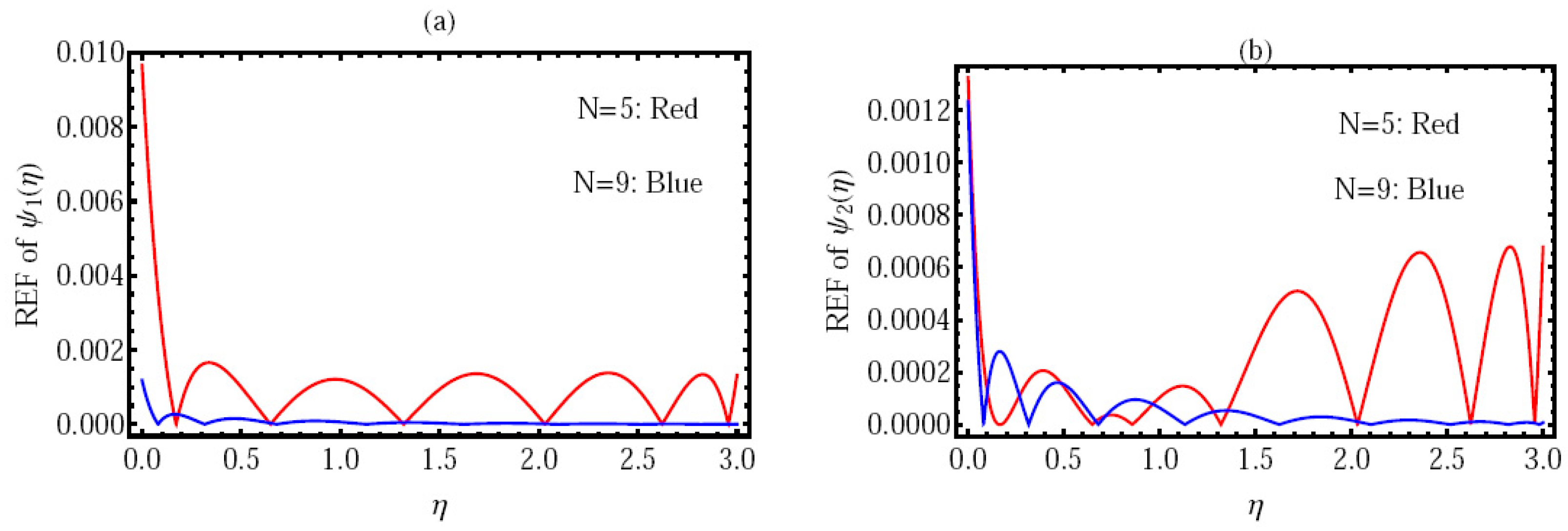
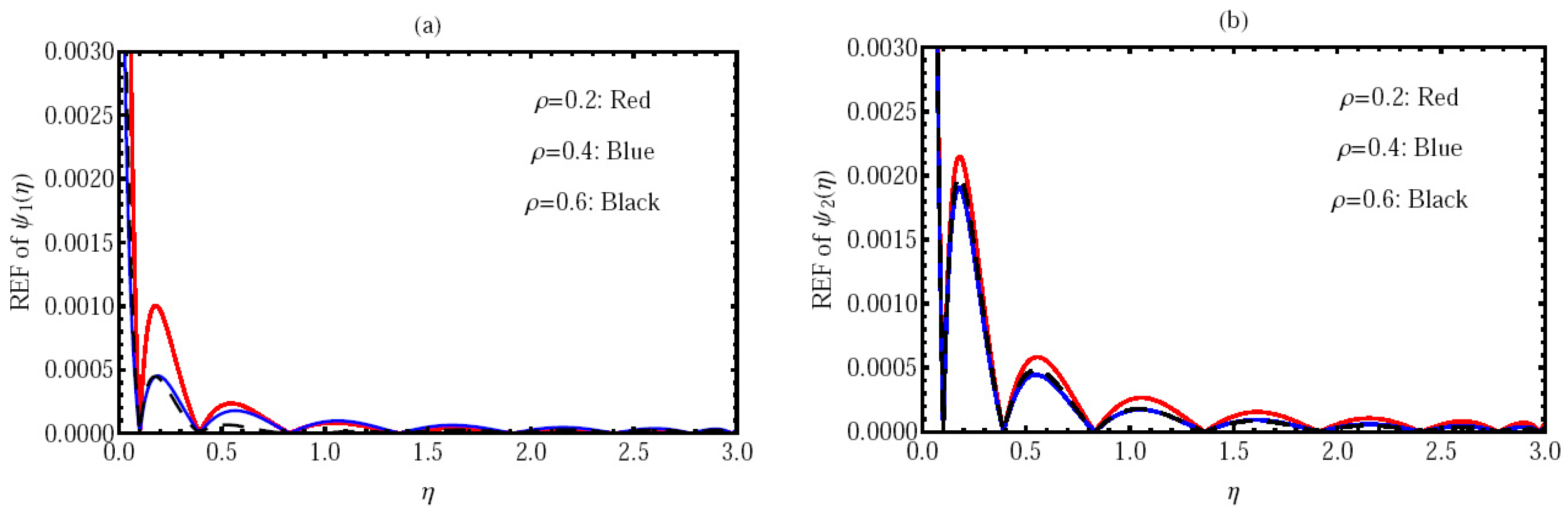
  • The following inequality applies to the error estimate norm ( L w ˜ 2 [ 0 , 1 ] -norm):
    ϕ ( η ) ϕ m ( η ) w ˜ < ε 12 m 3 .
  • The following absolute error bound applies if ϕ ( m ) ( η ) C [ 0 , 1 ] :
    ϕ ( η ) ϕ m ( η ) Δ Π m + 1 ( m + 1 ) ! π .
    Here, Δ = max η [ 0 , 1 ] ϕ ( m + 1 ) ( η ) and Π = max 1 η 0 , η 0 .
See the reference [22] for additional information on these polynomials and the convergence analysis for the approximation in (4).
Theorem 2.
The κ-order of the RFE fractional derivative for the function ϕ i ( η ) which is defined in Equation (4) can be evaluated as follows [20]:
R F E D κ ϕ i ( η ) = j = κ i χ i , j , κ [ G κ , p ( η , γ 0 ) + G κ , p ( η , γ m ) + 4 = 1 , o d d m 1 G κ , p ( η , γ ) + 2 = 2 , e v e n m 2 G κ , p ( η , γ ) ] ,
where
χ i , j , κ = h Γ ( i j + 1 ) 3 Γ ( i j + 1 κ ) × ( 1 ) j 2 i 4 i j Γ ( 2 i j ) Γ ( j + 1 ) Γ ( 2 i 2 j + 1 )
and
G κ , p ( η , γ ) = γ p κ R κ [ Ω ( η γ ) κ ] p = i j .
Proof. 
By using Theorem 1, we have
R F E D κ t i j = Γ ( i j + 1 ) Γ ( i j κ + 1 ) × h 3 [ G κ , p ( η , γ 0 ) + G κ , p ( η , γ m ) + 4 = 1 , o d d m 1 G κ , p ( η , γ ) + 2 = 2 , e v e n m 2 G κ , p ( η , γ ) ] .
Each segment in the domain [ 0 , 1 ] has a length of h and is divided into m equal segments. This fact yields that h = 1 m and γ = m for each = 0 , 1 , 2 , . . . , m , and
G κ , p ( η , γ ) = γ p κ R κ [ Ω ( t γ ) κ ] p = i j .
Now using Equations (4) and (7), we can evaluate the RFE derivative of ϕ i ( η ) as follows:
R F E D κ ϕ i ( η ) = j = 0 i ( 1 ) j 2 i 4 i j Γ ( 2 i j ) Γ ( j + 1 ) Γ ( 2 i 2 j + 1 ) R F E D κ η i j = j = κ i Γ ( i j + 1 ) Γ ( i j + 1 κ ) × ( 1 ) j 2 i 4 i j Γ ( 2 i j ) Γ ( j + 1 ) Γ ( 2 i 2 j + 1 ) × h 3 [ G κ , p ( η , γ 0 ) + G κ , p ( η , γ m ) + 4 = 1 , o d d m 1 G κ , p ( η , γ ) + 2 = 2 , e v e n m 2 G κ , p ( η , γ ) ] .
From this result, we can easily obtain the required Formula (6), as desired. □

3. Numerical Implementation

In this stage of our study, the approach designed in the previous section is used to numerically obtain a semi-analytical solution for the proposed fractional model. In this way, we drastically simplify the problem to a nonlinear system of algebraic equations. To obtain the unknown coefficients of the series solution, this system is converted into a restricted optimization problem. More precisely, we investigate the Brusselator system as formulated in an RFE-fractional form as follows ([17,18]):
R F E D ϱ ψ 1 ( η ) = ρ ( λ + 1 ) ψ 1 ( η ) + ψ 1 2 ( η ) ψ 2 ( η ) ,
R F E D ϱ ψ 2 ( η ) = λ ψ 1 ( η ) ψ 1 2 ( η ) ψ 2 ( η ) ,
ψ 1 ( 0 ) = ψ 1 , 0 , ψ 2 ( 0 ) = ψ 2 , 0 .
In this model, the parameters ρ > 0 , λ > 0 , and ψ 1 , 0 , ψ 2 , 0 are real constants [23]. These equations describe how the concentrations of the two species change over time due to the reaction and diffusion processes. The behavior of the Brusselator model (BM) depends critically on the values of the parameters ρ and λ . These parameters control the strength of the reaction and diffusion processes and, hence, determine the system’s overall behavior. In particular, the parameter ρ controls the distance from the Hopf bifurcation, a critical point at which the system transitions from a stable to an unstable steady state. The system can exhibit sustained oscillations as ρ increases beyond this critical value. Parameter λ controls the balance between the reaction and diffusion processes. The reaction dominates at low values of λ , and the system can exhibit sustained oscillations or spiral waves. As λ increases, diffusion becomes more important, and the system can exhibit Turing patterns.
As we pointed out, we use the approach proposed in this work to numerically solve the system (9)–(11). In the first stage, we approximate ψ 1 ( η ) and ψ 2 ( η ) by ψ 1 N ( η ) , and ψ 2 N ( η ) , respectively, in the following formulas:
ψ 1 N ( η ) = i = 0 N α i SVL i ( η ) , ψ 2 N ( η ) = i = 0 N β i SVL i ( η ) .
Now substituting (4) and (12) into the system (9)–(10) and evaluating them at the N points η s which are the roots of SVL N ( η ) , we obtain the identities
j = ϱ N α j χ N , j , ϱ [ G ϱ , p ( η s , γ 0 ) + G ϱ , p ( η s , γ m ) + 4 k = 1 , k o d d m 1 G ϱ , p ( η s , γ k ) + 2 k = 2 , k e v e n m 2 G ϱ , p ( η s , γ k ) ] = ρ ( 1 + λ ) i = 0 N α i SVL i ( η s ) + i = 0 N α i SVL i ( η s ) 2 i = 0 N β i SVL i ( η s ) ,
and
j = ϱ N β j χ N , j , ϱ [ G ϱ , p ( η s , γ 0 ) + G ϱ , p ( η s , γ m ) + 4 k = 1 , k o d d m 1 G ϱ , p ( η s , γ k ) + 2 k = 2 , k e v e n m 2 G ϱ , p ( η s , γ k ) ] = λ i = 0 N α i SVL i ( η s ) + i = 0 N α i SVL i ( η s ) 2 i = 0 N β i SVL i ( η s ) .
Substituting Equation (12) into (11), the initial conditions (11) are transformed into the following system of algebraic equations:
i = 0 N 2 ( 1 ) i α i = ψ 1 , 0 , i = 0 N 2 ( 1 ) i β i = ψ 2 , 0 .
As a consequence, the following cost functions (CFs) can be used to express the preceding system as a restricted optimization problem:
C F 1 = r = 0 N | j = ϱ N α j χ N , j , ϱ [ G ϱ , p ( η s , γ 0 ) + G ϱ , p ( η s , γ m ) + 4 k = 1 , k o d d m 1 G ϱ , p ( η s , γ k ) + 2 k = 2 , k e v e n m 2 G ϱ , p ( η s , γ k ) ] ρ + ( 1 + λ ) i = 0 N α i SVL i ( η s ) i = 0 N α i SVL i ( η s ) 2 i = 0 N β i SVL i ( η s ) | ,
and
C F 2 = r = 0 N | j = ϱ N β j χ N , j , ϱ [ G ϱ , p ( η s , γ 0 ) + G ϱ , p ( η s , γ m ) + 4 k = 1 , k o d d m 1 G ϱ , p ( η s , γ k ) + 2 k = 2 , k e v e n m 2 G ϱ , p ( η s , γ k ) ] λ i = 0 N α i SVL i ( η s ) + i = 0 N α i SVL i ( η s ) 2 i = 0 N β i SVL i ( η s ) | .
In this case, the constraint has the form
Cons = | i = 0 N 2 ( 1 ) i α i ψ 1 , 0 | + | i = 0 N 2 ( 1 ) i β i ψ 2 , 0 | .
We use the Penalty Leap Frog procedure [24] for solving the constrained optimization problem (16)–(18) for the unknowns α i and β i , for each i = 0 , 1 , 2 , . . . , N . This, in turn, leads us to formulate the approximate solution by substitution into (12).
The remainder of this section is devoted to presenting numerical simulations on a test example associated with system (9)–(11) in the range [ 0 , 3 ] , with varying values of N, ρ , and λ , and initial conditions ψ 1 , 0 = 1 and ψ 2 , 0 = 1 . As a result of our experiments, we confirm the accuracy and quality of the numerical scheme. Figure 1 illustrates the behavior of the approximation using several values of ϱ (namely, ϱ = 1.0 , 0.9 , 0.8 , 0.7 ), λ = 1 , ρ = 0.25 , and N = 8 . Figure 2 presents a comparison of our approach against the well-known fourth-order Runge–Kutta method (RK4), using ϱ = 1 , ρ = 0.25 , λ = 1 , and N = 8 . The behavior of the approximate solution employing the different values of λ = 0.5 , 1.0 , 1.5 , along with ϱ = 0.95 , N = 8 , and ρ = 0.25 , is presented in Figure 3. Also, the behavior of the approximate solution using the values ρ = 0.3 , 0.6 , 0.9 , and ϱ = 0.95 , N = 8 and λ = 1.0 is shown in Figure 4. From Figure 3 and Figure 4, we can confirm that the behavior of the BM depends critically on the values of the parameters λ and ρ . These parameters control the strength of the reaction and diffusion processes and, hence, determine the system’s overall behavior. In turn, Figure 5 shows the residual error function (REF) of the approximate solution using the values N = 5 , 9 , with ϱ = 0.95 , ρ = 0.1 and λ = 1 . Finally, Figure 6 presents the behavior of the REF for the approximate solution using ρ = 0.2 , 0.4 , 0.6 , along with ϱ = 0.95 , N = 8 , and λ = 0.5 . These results show the behavior of the numerical solution resulting from the application of the proposed method concerning the parameters ϱ , N, λ , and ρ . We observe that the proposed method is adequate for solving the proposed model in its fractional form with the RFE operator.

4. Conclusions

The Brusselator model is a simple yet powerful mathematical model of chemical reaction dynamics that has significantly impacted the field of chemical research. By understanding the behavior of this model, researchers can gain insights into the underlying mechanisms of chemical reactions and develop new strategies for controlling and manipulating these reactions. This model is an important example of a nonlinear dynamical system and has applications in various fields beyond chemistry. In this manuscript, the numerical solutions for the fractional Brusselator model were calculated using the Rabotnov fractional-exponential kernel fractional derivative. Various fractional orders were considered, and we employed the residual error function in our investigation. The results confirmed that the proposed method is suitable for approximating the fractional mathematical model considered in this work. Additionally, by including additional terms from the approximation solution series, we were able to control the precision of the error and decrease it conveniently. Moreover, we concluded that the numerical simulations of the model under consideration in the current study are better suited for the RFE operator without singularity. By assessing the residual error function, we confirmed the effectiveness and accuracy of the proposed approach. As a future generalization of this work, we will attempt to deal with the same problem using a different kind of fractional derivative and different type of polynomials. Finally, we must point out that the Mathematica software program was used to carry out the numerical simulation work.

Author Contributions

Conceptualization, M.M.K., J.E.M.-D., K.M.S. and W.M.H.; methodology, M.M.K., J.E.M.-D., K.M.S. and W.M.H.; software, M.M.K., J.E.M.-D., K.M.S. and W.M.H.; validation, M.M.K., J.E.M.-D., K.M.S. and W.M.H.; formal analysis, M.M.K., J.E.M.-D., K.M.S. and W.M.H.; investigation, M.M.K., J.E.M.-D., K.M.S. and W.M.H.; resources, M.M.K., J.E.M.-D., K.M.S. and W.M.H.; data curation, M.M.K., J.E.M.-D., K.M.S. and W.M.H.; writing—original draft preparation, M.M.K., J.E.M.-D., K.M.S. and W.M.H.; writing—review and editing, M.M.K., J.E.M.-D., K.M.S. and W.M.H.; visualization, M.M.K., J.E.M.-D., K.M.S. and W.M.H.; supervision, M.M.K., J.E.M.-D., K.M.S. and W.M.H.; project administration, M.M.K., J.E.M.-D., K.M.S. and W.M.H.; funding acquisition, J.E.M.-D. All authors have read and agreed to the published version of the manuscript.

Funding

The corresponding author, J.E.M.-D., wishes to acknowledge the financial support from the National Council of Science and Technology of Mexico (CONACYT) through grant A1-S-45928.

Institutional Review Board Statement

Not applicable.

Informed Consent Statement

Not applicable.

Data Availability Statement

The data that support the findings of this study are available from the corresponding author, J.E.M.-D., upon reasonable request.

Conflicts of Interest

The authors declare no conflict of interest.

References

  1. Kilbas, S.G.; Kilbas, A.A.; Marichev, O.I. Fractional Integrals and Derivatives: Theory and Applications; Gordon & Breach: New York, NY, USA, 1993. [Google Scholar]
  2. Diethelm, K. An algorithm for the numerical solution of differential equations of fractional order. Electron. Trans. Numer. Anal. 1997, 5, 1–6. [Google Scholar]
  3. Khader, M.M.; Adel, M. Numerical study of the fractional modeling on SIR equations with constant vaccination rate using GEM. Int. J. Nonlinear Sci. Numer. Simul. 2019, 20, 69–76. [Google Scholar] [CrossRef]
  4. Podlubny, I. Fractional Differential Equations; Academic Press: San Diego, CA, USA, 1999. [Google Scholar]
  5. Gao, W.; Ghanbari, B.; Baskonus, H.M. New numerical simulations for some real-world problems with Atangana-Baleanu fractional derivative. Chaos Solitons Fractals 2019, 128, 34–43. [Google Scholar] [CrossRef]
  6. Morales-Delgado, V.F.; Gomez-Aguilar, J.F.; Saad, K.M.; Escobar-Jimenez, R.F. Application of the Caputo-Fabrizio and Atangana-Baleanu fractional derivatives to the mathematical model of cancer chemotherapy effect. Math. Methods Appl. Sci. 2019, 42, 1167–1193. [Google Scholar] [CrossRef]
  7. Toufik, M.; Atangana, A. New numerical approximation of fractional derivative with the non-local and non-singular kernel: Application to chaotic models. Eur. Phys. J. Plus 2017, 132, 1–14. [Google Scholar] [CrossRef]
  8. Kumar, D.; Singh, J.; Baleanu, D. On the analysis of vibration equation involving a fractional derivative with Mittag-Leffler law. Math. Methods Appl. Sci. 2020, 43, 443–457. [Google Scholar] [CrossRef]
  9. Saad, K.M.; Khader, M.M.; Gomez-Aguilar, J.F.; Baleanu, D. Numerical solutions of the fractional Fisher’s type equations with Atangana-Baleanu fractional derivative by using spectral collocation methods. Chaos 2019, 29, 1–5. [Google Scholar] [CrossRef]
  10. Srivastava, H.M.; Gusu, D.M.; Mohammed, P.O.; Wedajo, G.; Nonlaopon, K.; Hamed, Y.S. Solution of general fractional-order differential equations by using the spectral Tau method. Fractal Fract. 2022, 6, 7. [Google Scholar] [CrossRef]
  11. Youssri, Y.H.; Abd-Elhameed, W.M.; Ahmed, H.M. New fractional derivative expression of the shifted third-kind Chebyshev polynomials: Application to a type of nonlinear fractional pantograph differential equations. J. Funct. Spaces 2022, 2022, 3966135. [Google Scholar] [CrossRef]
  12. Doha, E.H.; Abd-Elhameed, W.M.; Ahmed, H.M. The coefficients of differentiated expansions of double and triple Jacobi polynomials. Bull. Iran. Math. Soc. 2012, 38, 739–766. [Google Scholar]
  13. Abd-Elhameed, W.M.; Youssri, Y.H. Connection formulae between generalized Lucas polynomials and some Jacobi polynomials: Application to certain types of fourth-order BVPs. Int. J. Appl. Comput. Math. 2020, 6, 1–19. [Google Scholar] [CrossRef]
  14. Agarwal, F.; El-Sayed, A.A. Vieta-Lucas polynomials for solving a fractional-order mathematical physics model. Adv. Differ. Equ. 2020, 2020, 1–18. [Google Scholar] [CrossRef]
  15. Adel, M.; Khader, M.M.; Assiri, T.A.; Kallel, W. Numerical simulation for COVID-19 model using a multidomain spectral relaxation technique. Symmetry 2023, 15, 931. [Google Scholar] [CrossRef]
  16. Alesemi, M. Numerical analysis of fractional-order parabolic equation involving Atangana-Baleanu derivative. Symmetry 2023, 15, 237. [Google Scholar] [CrossRef]
  17. Gafiychuk, V.; Datsko, B. Stability analysis and limit cycle in the fractional system with Brusselator nonlinearities. Phys. Lett. A 2008, 372, 4902–4904. [Google Scholar] [CrossRef]
  18. Wang, Y.; Li, C. Does the fractional Brusselator with efficient dimension less than 1 have a limit cycle? Phys. Lett. A 2007, 363, 414–419. [Google Scholar] [CrossRef]
  19. Atangana, A.; Baleanu, D. New fractional derivative with non-local and non-singular kernel. Therm. Sci. 2016, 20, 736–769. [Google Scholar] [CrossRef]
  20. Kumar, S.; Gomez-Aguilar, J.F.; Lavin-Delgado, J.E.; Baleanu, D. Derivation of operational matrix of Rabotnov fractional-exponential kernel and its application to fractional Lienard equation. Alex. Eng. J. 2020, 56, 991–2997. [Google Scholar] [CrossRef]
  21. Horadam, A.F. Vieta Polynomials; The University of New England: Armidaie, VC, Australia, 2000. [Google Scholar]
  22. Zakaria, M.; Khader, M.M.; Al-Dayel, I.; Al-Tayeb, W. Solving fractional generalized Fisher-Kolmogorov-Petrovsky-Piskunov’s equation using compact finite different method together with spectral collocation algorithms. J. Math. 2022, 2022, 1901131. [Google Scholar]
  23. Jafari, H.; Abdelouahab, K.; Baleanu, D. Variational iteration method for a fractional-order Brusselator system. Abstr. Appl. Anal. 2014, 2014, 496323. [Google Scholar] [CrossRef]
  24. El-Hawary, H.M.; Salim, M.S.; Hussien, H.S. Ultraspherical integral method for optimal control problems governed by ordinary differential equations. J. Glob. Optim. 2003, 25, 283–303. [Google Scholar] [CrossRef]
Figure 1. Approximate solutions for (a) ψ 1 ( η ) and (b) ψ 2 ( η ) vs. different values of ϱ .
Symmetry 15 01619 g001
Figure 2. Solutions for (a) ψ 1 ( η ) and (b) ψ 2 ( η ) using the proposed approach and the RK4 method.
Symmetry 15 01619 g002
Figure 3. Approximate solutions for (a) ψ 1 ( η ) and (b) ψ 2 ( η ) vs. different values of λ .
Symmetry 15 01619 g003
Figure 4. Approximate solutions for (a) ψ 1 ( η ) and (b) ψ 2 ( η ) vs. different values of ρ .
Symmetry 15 01619 g004
Figure 5. The REF for the solutions (a) ψ 1 ( η ) and (b) ψ 2 ( η ) vs. different values of N.
Symmetry 15 01619 g005
Figure 6. The REF of the solutions (a) ψ 1 ( η ) and (b) ψ 2 ( η ) vs. different values of ρ .
Symmetry 15 01619 g006
Disclaimer/Publisher’s Note: The statements, opinions and data contained in all publications are solely those of the individual author(s) and contributor(s) and not of MDPI and/or the editor(s). MDPI and/or the editor(s) disclaim responsibility for any injury to people or property resulting from any ideas, methods, instructions or products referred to in the content.

