Fuzzy Model Parameter and Structure Optimization Using Analytic, Numerical and Heuristic Approaches

Abstract

Fuzzy systems are widely used in most fields of science and engineering, mainly because the models they produce are robust, accurate, easy to evaluate and capture real-world uncertainty better than do the classical alternatives. We propose a new methodology for structure and parameter tuning of Takagi–Sugeno–Kang fuzzy models using several optimization techniques. The output parameters are determined analytically, by finding the minimum of the root-mean-square error (RMSE) for a properly defined error function. The membership functions are simplified by considering symmetry and equispacing, to reduce the optimization problem of finding their parameters, and allow it to be carried out using the numerical method of gradient descent. Both algorithms are fast enough to finally implement a strategy based on the hill climbing approach to finding the optimal structure (number and type of membership functions) of the fuzzy system. The effectiveness of the proposed strategy is shown by comparing its performance, using four case studies found in current relevant works, to the popular adaptive network-based fuzzy inference system (ANFIS), and to other recently published strategies based on evolutionary fuzzy models. In terms of the RMSE, performance was at least 28% better in all case studies.

1. Introduction

This work proposes an optimization strategy that combines three different approaches: heuristic; numerical; and analytic optimization. The aim was to produce a synergy, to determine the parameters and structure of a Takagi–Sugeno–Kang fuzzy-rule-based system. The combination of these approaches is intended to maximize the advantages and to minimize the disadvantages that each of them possesses on their own.

Fuzzy systems are a numerical modeling technique fitted to experimental data, which are widely used [1]. The distinction of fuzzy systems is the use of fuzzy sets, which possess the characteristic that their elements may belong to them partially (in a degree of membership), thus capturing the natural imprecision of human knowledge [2].

One of the advantages of fuzzy models is that they can express a highly nonlinear functional relationship, even with a small number of rules [3]: this characteristic is relevant, given that nonlinear systems are widespread in practice.

Fuzzy systems have been categorized into three types, based on their consequent part rules [4]: the first type is Mamdani, which uses IF–THEN rules associated with linguistic variables, where the consequent part is within a fuzzy variable [5]; secondly, there are the Takagi–Sugeno–Kang (TSK) fuzzy systems, which use functional consequents (a linear combination of the entries) [6,7]; thirdly, there are singleton-type fuzzy systems, where, for each rule, a real number is assigned [4].

All three types of fuzzy systems have a universal approximation capacity for any nonlinear function [8]. Nevertheless, in comparison to the other two types, TSK fuzzy modeling can significantly decrease the number of fuzzy rules, particularly for complex systems with high dimensions [4].

TSK fuzzy systems include a set of rules [6]:

$$\begin{array}{c}{R}_l:\mathrm{If}{x}_1\mathrm{is}{F}_1\mathrm{and}\dots \mathrm{and}{x}_n\mathrm{is}{F}_n\end{array}$$

(1)

$$\begin{array}{c}\mathrm{Then}{z}_l=C_{l,1}{x}_1+\dots C_{l,n}{x}_n+C_{l,n+1},\end{array}$$

(2)

where x is the vector of the premise variables defined as $x=[x_1\dots x_n]$, $F_i$ is the fuzzy sets, $z_l$ is the output of the $R_l$ rule and $C_{l,k}$ is the kth coefficient associated with the $R_l$ rule. The antecedent part of the rule is known as (1), and the consequent part of the rule is known as (2). In addition to the output $z=\left\{z_i\right\}$ of each rule, it is necessary to calculate the degree of truth $\omega =\left\{{\omega }_i\right\}$ of all the rules, to compute the output of a TSK fuzzy logic system.

There are two main stages required to model a fuzzy system: identifying its structure, and optimizing its parameters. Identifying a fuzzy system’s structure involves determining how to partition the input–output space, and deciding the number of rules the system should use. Optimizing a fuzzy system’s parameters focuses on finding the best values for all the parameters in the system, including defining the fuzzy partitions and coefficients of each rule’s consequent part [9].

In our proposed strategy, the heuristic part is used to determine the structure of the model. Then, for each candidate structure, a gradient-based approach is used to search for the optimal antecedent parameters: this is done while applying an analytic approach to finding the corresponding optimal consequent parameters for each point in the search space.

The main contributions of this work are summarized as follows:

• This work presents a method based on optimization, to obtain the parameters of the antecedent and consequent parts and the appropriate structure of the fuzzy system;
• This work provides a fast analytic strategy for finding the optimal parameters of the consequent part for each set of parameters of the antecedent part, which sidesteps the current method found in the literature, of searching through a long set of parameters for the antecedent and consequent part simultaneously;
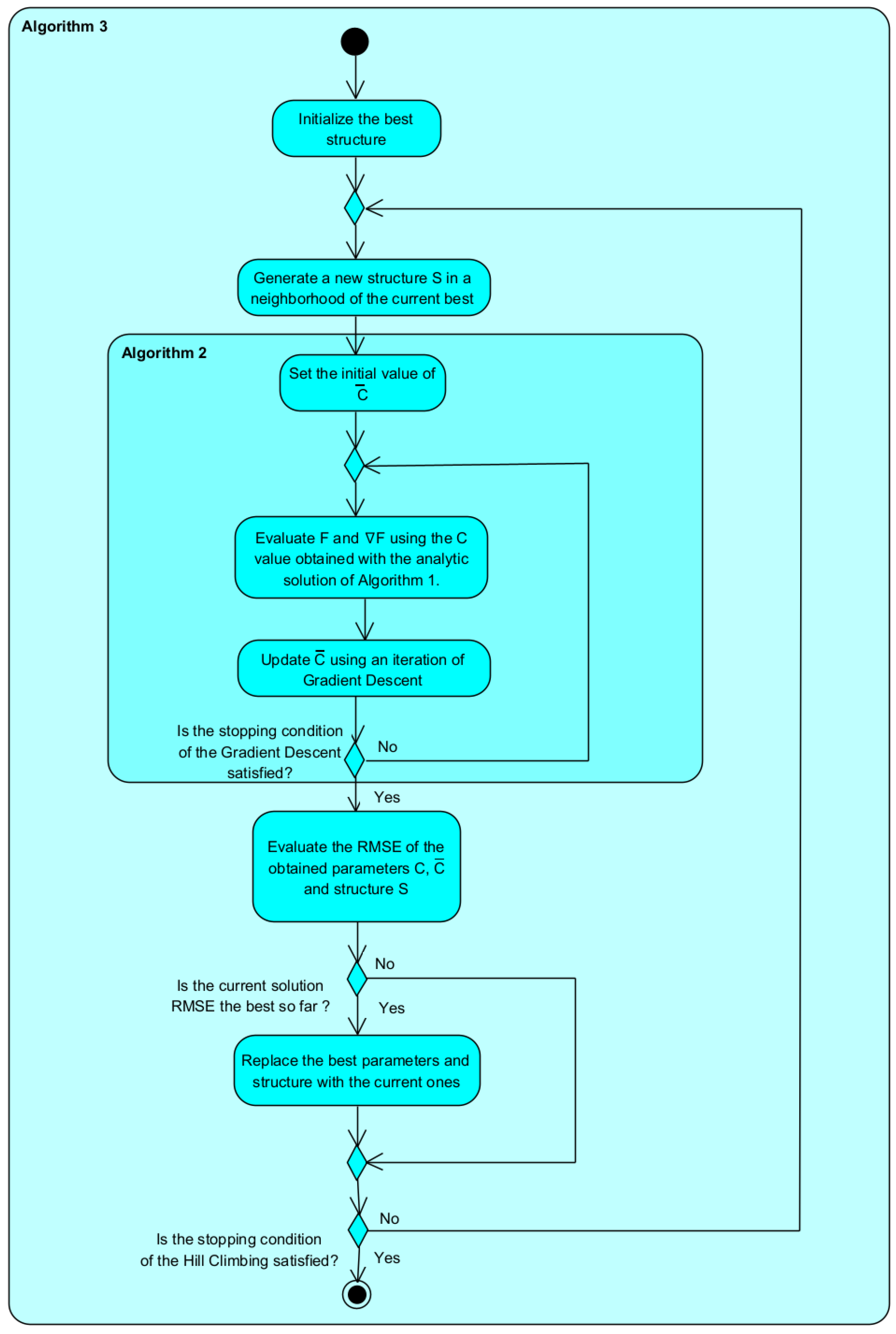
• This work proposes a hill climbing heuristic strategy to determine the optimal structure. This strategy uses, as a fitness function, the RMSE found with the algorithm that optimizes the parameters of the antecedent part.

A novel aspect of this work is that it reduces the number of parameters of the antecedent part, by considering only some particular classes of membership functions, i.e., triangular and Gaussian with symmetry and equispacing properties: this makes the optimization problem, of tuning the parameters, more manageable.

Section 2 and Section 3 present a brief literature overview of fuzzy systems tuning, and introduce the proposed strategy. Section 4 presents the four case studies that we used, to compare our strategy to others. Finally, a discussion of the case studies, and the conclusions from this work, are presented in Section 5 and Section 6.

2. Literature Overview

Fuzzy systems and some other related techniques have been used extensively in recent decades, to model complex systems. Initially, these systems were designed using only expert knowledge. Most research on optimizing fuzzy systems focuses on a fixed structure, and suggests methods for optimizing the system’s parameters within that structure, rather than changing the structure itself.

The initial methods for tuning fuzzy controllers relied on trial and error, as described in the earliest publications [10,11]. Subsequently, input and output data began to be used to adjust the parameters of the fuzzy controller [12].

More advanced approaches were based on numerical methods or neuro-fuzzy hybrid systems [13,14,15]; however, the majority of these strategies considered a fixed topology.

Greater effort was invested in solving the parameter tuning problem, as determining the system structure was a more complex and difficult task, which rendered it challenging to find effective methods or techniques. Another issue was that system structure identification algorithms could not be tested without employing parameter fitting algorithms. Consequently, both problems needed to be addressed at the same time.

Takagi and Sugeno presented the first relevant strategy in 1985 [6]. They optimized the consequents of fuzzy rules, using the least squares algorithm, and calculated the antecedents, using the complex method. Then, they applied a heuristic combinational approach to partitioning the input domain, resulting in more intricate topologies that could be optimized subsequently.

Neural networks with effective learning algorithms emerged in the late 1990s, as a substitute for automating or supporting the development of techniques for fine-tuning fuzzy systems [16,17,18,19].

Most of the early applications of these algorithms were in process control; however, their use gradually expanded, to include many other fields, e.g., fault detection, classification, data analysis and support for decision-making systems.

A set of fuzzy rules can be considered as a neuro-fuzzy system, which, like fuzzy rules, can be constructed solely based on input–output data, or can be initiated by existing knowledge. By merging fuzzy systems with neural networks, a final system was formed that offered the advantages of pattern learning and uncomplicated functionality interpretation [20,21].

Neuro-fuzzy systems can be represented using neural networks that perform logical operations. While it is not necessary to use a neural network to represent the parameters of a fuzzy system, according to some authors, this approach is considered more convenient, because it enables the visualization of the input flow within the system, as well as the error signals that are utilized to modify its parameters.

There are multiple neuro-fuzzy architectures, including the Fuzzy Adaptive Learning Control Network (FALCON), Generalized Approximate Reasoning-based Intelligence Control (GARIC), the Fuzzy Net (FUN), the Self-Constructing Neural Fuzzy Inference Network (SONFIN), the Neuronal Fuzzy Controller (NEFCON), the Fuzzy Inference and Neural Network in Fuzzy Inference Software (FINEST), the Fuzzy Neural Network (NFN), the Dynamic/Evolving Fuzzy Neural Network (EFuNN and dmEFuNN) and the Adaptive Network-based Fuzzy Inference System (ANFIS) [14,16,19,22,23,24,25,26,27,28,29].

ANFIS is a Takagi–Sugeno fuzzy inference system that uses the least mean square method to identify the consequent parameters, and backpropagation learning to detect input membership function parameters [14,30]. The iterative learning algorithm consists of two steps: firstly, the premises parameters are set and the input patterns are propagated, to determine the consequent parameters, using the iterative minimum squared method algorithm; secondly, the input patterns are propagated again, and the learning algorithm backpropagation is applied in each iteration, to adjust the premises parameters while keeping the consequents constant. Due to its immense popularity, and its frequent use in recent articles on fuzzy systems [31,32,33,34,35], and despite it not being a recent strategy, we decided to compare ANFIS to our proposal.

The rising interest in adaptive system modeling has driven the advancement of highly adaptable fuzzy systems, which are also referred to as evolving fuzzy systems (eFS): these models are self-developed from a continuous flow of data [36]. There are numerous alternative approaches, in the literature, to creating and implementing eFS: most of them propose systems based on evolutionary functional principles, in which the structure and/or the antecedent and consequent parameters evolve continually. These methods have been effectively utilized in a variety of fields, including system identification, pattern recognition and intelligent control [37,38,39,40,41].

A recent and favored strategy is the use of online learning fuzzy neural networks (FNNs), in which all neurons are generated and evolved continuously, by adapting them to the incoming data: this means that the neuron is included or modified by using various evolving mechanisms, to keep pace with the system’s behavior.

Due to the current popularity of such strategies, we decided to compare the performance of FNNs proposed in some recent articles [42,43,44,45,46,47,48,49,50,51,52,53,54,55,56,57,58,59,60] to that of our strategy.

3. Proposed Methodology

Our strategy can be interpreted as three optimization algorithms contained within each other: an analytical; a numerical; and a heuristic algorithm, each with a specific objective:

• Consequent coefficients determination;
• Antecedent parameter determination;
• Structural parameter determination.

The innermost algorithm—the analytical algorithm—finds the best parameters of the consequent part C for a fixed antecedent part and structure.

The analytical solution is not an approximation, but rather a precise representation of the solution. The calculations involved in obtaining the analytical solution are also faster, compared to iterative numerical methods or heuristic approaches. It is important to note that analytical solutions are not always feasible or available. Many complex real-world problems do not have known analytical solutions, due to their intricacy, their non-linearity, or the absence of mathematical models: in such cases, numerical or heuristic methods provide valuable alternatives for obtaining approximate or satisfactory solutions efficiently.

The second algorithm—the numerical algorithm—uses the numerical method of gradient descent to find the best parameters of the antecedent part $\overline{C}$, considering the fixed structure, with the help of the analytical algorithm.

Numerical methods aim to find precise or accurate solutions, by employing systematic mathematical techniques, and often involve iterative processes, convergence analysis and error estimation. In particular, gradient descent involves computing the gradient of a cost or objective function with respect to the parameters, and using it as the search direction. The simplicity of the algorithm makes it accessible and efficient to use. While gradient descent is widely used, there are certain scenarios where its application may not be suitable or effective: for example, for non-differentiable functions or in the case of combinatorics problems, such as determining the structure.

The third and outermost algorithm is the main algorithm, a hill climber that calculates the fitness of each structure as the RMSE of the best possible parameters $C,\overline{C}$, by using the second algorithm.

Hill climbing is known to be computationally efficient, as it does not require complex mathematical models; moreover, it does not rely on explicit gradient information, and it strikes a balance between exploration and exploitation. Despite these advantages, it is important to note that hill climbing has some limitations typical of heuristic algorithms: unlike deterministic algorithms that guarantee an optimal solution, heuristic methods trade accuracy for efficiency; hill climbing can get trapped in a local optimum, and may struggle to find the global optimum in complex problem landscapes.

A general activity diagram of the proposal can be seen in Figure 1.

The following sections explain each of the algorithms in detail, and the process of finding the parameters of the consequent part, using calculus.

3.1. Consequent Coefficients Determination

Before solving these problems, min–max normalization was applied to the dataset, to prevent values in a larger interval from having a bigger influence on the model’s output, as occurs in some machine learning strategies [58].

The output $\overline{y}$ of a TSK fuzzy system is calculated as the weighted average of the rules outputs, considering their degree of truth:

$$\begin{array}{c}\overline{y}=\frac{{\sum }_{l=1}^R{\omega }_l{z}_l}{{\sum }_{l=1}^R{\omega }_l}\end{array}$$

(3)

where R is the number of rules, and ${\omega }_l$ is the degree of truth of the lth rule.

To formulate the problem of finding the set of parameters $C_{i,j}$ as an optimization problem, an error function is defined—in this case, the previously named RMSE:

$$\begin{array}{c}RMSE=\sqrt{\frac{{\sum }_{j=1}^{n_d}{(\overline{y}-y)}^2}{n_d}},\end{array}$$

(4)

where y was the output of the dataset. As $n_d$ (the number of observations) was constant, and as the root argument was always positive, the minimum of the RMSE was also the minimum of the simpler function E:

$$\begin{array}{c}E:=\sum _{j=1}^{n_d}{(\overline{y}-y)}^2.\end{array}$$

(5)

Considering that the structure was fixed, and that the set of points was given, it was possible to calculate the partial derivatives of E with respect to the consequent parameters, and to solve the problem of finding the parameters that minimized the error directly.

Using

$$\begin{array}{c}\frac{\partial E}{\partial \overline{y}}=\sum _{j=1}^{n_d}2(\overline{y}-y),\end{array}$$

(6)

$$\begin{array}{c}\frac{\partial \overline{y}}{\partial z_k}=\frac{\omega }{{\sum }_{l=1}^m{\omega }_l},\end{array}$$

(7)

and

$$\begin{array}{c}\frac{\partial z_k}{\partial C_{k,m}}=x_m\ast =\left\{\begin{array}{ccc}{x}_m\hfill & if& m\le n\\ 1\hfill & if& m=n+1,\end{array}\right.\end{array}$$

(8)

it was possible to use the chain rule to calculate

$$\begin{array}{c}\frac{\partial E}{\partial C_{k,m}}=\sum _{j=1}^{n_d}2(\overline{y}-y)\frac{\omega }{{\sum }_{l=1}^R{\omega }_l}{x}_m\ast .\end{array}$$

(9)

Substituting $\overline{y}$ from (3) in (9), we obtained

$$\begin{array}{c}\frac{\partial E}{\partial C_{k,m}}=\sum _{j=1}^{n_d}2\left(\frac{{\sum }_{l=1}^R{\omega }_l{z}_l}{{\sum }_{l=1}^R{\omega }_l}-y\right)\frac{\omega }{{\sum }_{l=1}^m{\omega }_l}{x}_m\ast ,\end{array}$$

(10)

and substituting $z_l$ from (2) with the definition $S:={\sum }_{l=1}^R{\omega }_l$, we could write

$$\begin{array}{c}\frac{\partial E}{\partial C_{k,m}}=\end{array}$$

(11)

$$\begin{array}{c}\frac{2{\omega }_k}{S}\sum _{j=1}^{n_d}-\left(y^j{x}_m^j\right)+\frac{2{\omega }_k}{S^2}\sum _{j=1}^{n_d}\left(\sum _{i=1}^R{\omega }_l\sum _{l=1}^{n+1}{C}_{i,l}{x}_l^j\right)x_m\ast ,\end{array}$$

(12)

when the notation $x_i^j$ was the ith variable of the jth observation in the dataset.

Alternatively, if we defined E in terms of the error of each observation $e_j:={(\overline{y}-y)}^2$ as

$$\begin{array}{c}E=\sum _{j=1}^{n_d}{e}_j\end{array}$$

(13)

we could evaluate

$$\begin{array}{c}\frac{\partial e_j}{\partial C_{k,m}}=-\frac{2{\omega }_k}{S}\left(y^j{x}_m^j\right)+\frac{2{\omega }_k{x}_m\ast }{S^2}\sum _{i=1}^R{\omega }_l\sum _{l=1}^{n+1}{C}_{i,l}{x}_l\end{array}$$

(14)

or

$$\begin{array}{c}\frac{\partial e_j}{\partial C_{k,m}}=k_j+a_{1,1}{C}_{1,1}+a_{1,2}{C}_{1,2}+\cdots +a_{R,n+1}{C}_{R,n+1},\end{array}$$

(15)

where

$$\begin{array}{c}{k}_j=-\frac{2{\omega }_k}{S}\left(y^j{x}_m^j\right)\end{array}$$

(16)

and

$$\begin{array}{c}{a}_{i,l}=\frac{2{\omega }_k}{S^2}\left(x_m^j{\omega }_i{x}_l\right);\end{array}$$

(17)

then, it was possible to express the gradient vector of $e_j$ with respect to the parameters C as the sum of a constant term, $K_j$, with a linear combination of the parameters C, i.e., there was a matrix $A_j\in M_{R(n+1)xR(n+1)}$ and a vector $K_j\in {\mathbb{R}}^{R(n+1)}$, such that

$$\begin{array}{c}\nabla e_j=\left[\begin{array}{c}\frac{\partial e_j}{\partial C_{1,1}}\\ ⋮\\ \frac{\partial e_j}{\partial C_{R,n+1}}\end{array}\right]=K_j+A_{j}C,\end{array}$$

(18)

and, after computing $e_j$ for each observation, the gradient of the error E could be calculated as

$$\begin{array}{c}\nabla E=\sum _{j=1}^{n_d}\nabla e_j=\sum _{j=1}^{n_d}(K^j+A^{j}C)\end{array}$$

(19)

or

$$\begin{array}{c}\nabla E=\left[\begin{array}{c}\frac{\partial E}{\partial C_{1,1}}\\ ⋮\\ \frac{\partial E}{\partial C_{R,n+1}}\end{array}\right]=K+AC,\end{array}$$

(20)

where $A={\sum }_{j=1}^{n_d}{A}^j$ and $K={\sum }_{j=1}^{n_d}{K}^j$.

As E was a convex function (5), E had a minimum that was well-defined with respect to the parameters C when $\nabla E=0$, i.e., when

$$\begin{array}{c}C=-A^{-1}K.\end{array}$$

(21)

Thus, for a fixed antecedent part, it was possible to calculate the parameters of the consequent part that minimized the RMSE analytically, by calculating the contribution to A and K from each observation in a cycle, and subsequently solving a system of equations.

Furthermore, if we stored the matrix A and the vector K, it was possible to update the set of optimal weights when a new observation arrived, tuning the system online, without having to reset the whole calculation or to use the previous observations, simply by adding the contribution of the new data to A and K, and solving the new linear system.

The procedure for tuning the consequent part parameters is shown in Algorithm 1.

Algorithm 1 Obtaining the optimal consequent parameters C

Minmax(x,y). Set A = 0, K = 0; for j = 0 to $n_d$ do    Calculate the membership of $\mu \left(x\right)$ to each class.    Calculate the degree of truth of each rule $\omega \left(\mu \right)$.    Evaluate $A_j(x^j,\omega ),K_j(x^j,y^j,\omega )$    $A=A+A_j$ and $K=K+K_j$ end for $C=-A^{-1}K$ return C

3.2. Antecedent Parameter Determination

The membership functions type that we used was called ’structure’. Considering that, for the described problem, both the number of fuzzy partitions for each variable and the structure were fixed, the objective was then to determine the parameters for each of them.

In order to reduce the number of parameters, and to solve the problem optimally, it was decided to force the membership functions to be symmetric, with equispaced centers, as shown in Figure 2. As the data were normalized between 0 and 1, in the case of using two membership functions, their centers would be found at 0 and 1, while for three membership functions, their centers would be at 0, 0.5 and 1, respectively. In general, the ith centroid $\theta$ position was computed using Equation (22), where p was the number of fuzzy sets in the partition:

$$\begin{array}{c}{\displaystyle {\theta }_i=\frac{i-1}{p-1}.}\end{array}$$

(22)

This last consideration was not arbitrary: the tuning process of multiple strategies, such as ANFIS, usually brings the centers to values close to equidistance. Some authors [59] tend to recommend the use of normal membership functions with the unit at the extreme values, such as those produced by this approach.

The symmetry condition allowed us to reduce the number of parameters by half, in the case of triangular functions. By knowing their center and forcing symmetry, we would only have to determine one parameter: the limit of the set related to the percentage of overlap between neighboring sets. In the case of Gaussian bells, the parameter to be determined would be the variance.

We denoted $\overline{C}$ as the set of parameters of the membership functions, a vector of length m, whose components represented the percentage of overlap of each membership function with its neighbor. The objective was to minimize the RMSE, which depended also on the parameters C of the consequent part:

$$\begin{array}{c}{\displaystyle \underset{C,\overline{C}}{min}RMSE(C,\overline{C}).}\end{array}$$

(23)

The proposed approach was to find the optimal C for a fixed $\overline{C}$, and to use that RMSE value as the fitness function of $\overline{C}$:

$$\begin{array}{c}{\displaystyle F\left(\overline{C}\right):=\underset{C}{min}RMSE\left(C\right)\mathrm{with}\mathrm{fixed}\overline{C}.}\end{array}$$

(24)

The objective function was the minimum RMSE obtained by the process explained in the previous section. As it was necessary to go through all the observations, and to solve a large system of equations to evaluate the fitness, and as this was computationally expensive, the use of heuristic strategies that required multiple evaluations was discarded.

For this reason, in addition to other advantages of numerical methods—such as their solid theoretical foundation—a numerical method was adopted. In particular, it was decided to use the gradient descent method, because, despite its low order of convergence, it did not require the use of a numerical estimation of a Hessian matrix or many fitness function evaluations, which were considered expensive and unstable.

An overlap between neighboring fuzzy sets of between 10% and 50% had to be ensured, to obtain uniform and stable performance [61]; therefore, it was decided to use ${\overline{C}}_0$ as the starting value = $0.25$: that is, initially, each fuzzy set had a 25% overlap with its neighbors.

The algorithm worked by taking small steps from ${\overline{C}}_0$ in the direction of the steepest decline of the cost function, $F\left(\overline{C}\right)$, which was given by the negative gradient of the cost function itself.

At each iteration, the algorithm computed the gradient of the cost function with respect to the current parameter $\overline{C}$ values, and then updated the parameters, by subtracting a fraction of the gradient $\alpha$, known as the learning rate. The learning rate determined the step size at each iteration of the algorithm. The step size had to be accurate: if it was too large, the algorithm might overshoot the minimum, and fail to converge; if it was too small, the convergence might be slow.

To estimate the value of $\alpha$, it was decided to use a backtracking algorithm. At each iteration, the algorithm checked whether the current value of the objective function had decreased sufficiently: if it had not decreased, the algorithm reduced the learning rate, by multiplying it by a small constant value $\beta$, and repeated this process until the current value of the objective function had decreased sufficiently.

The gradient descent implemented can be formulated as shown in Algorithm 2.

Algorithm 2 Gradient descent

Set $k=0,{\overline{C}}_k=0.25,\beta =0.5$ and $ϵ>0$ while  $\left|\right|\overrightarrow{\nabla }F\left({\overline{C}}_k\right)\left|\right|>ϵ$  do    $\alpha =1$    repeat      $\alpha =\beta \alpha$    until $F({\overline{C}}_k+\alpha \overrightarrow{\nabla }F\left({\overline{C}}_k\right))<F\left({\overline{C}}_k\right)$    ${\overline{C}}_{k+1}={\overline{C}}_k-\alpha \nabla F\left({\overline{C}}_k\right)$ end while return  ${\overline{C}}_k$

3.3. Structural Parameter Determination

An empirical consideration that had to be followed for the conformation of the fuzzy sets was that the number of fuzzy sets associated with a variable had to be between two and nine [61].

It is considered advisable to use odd values, so as to always have an inflection set [61]; however, from practical experience, an even number is sometimes preferable, in terms of the RMSE: therefore, this last consideration was not taken into account.

At this stage, the suitability of a structure was calculated as the result of applying the algorithm described in the previous stage for the given structure, i.e., to determine the fitness of a structure, the parameters of the optimal antecedent part were found, as in the previous step, and, with them, the parameters of the consequent part were found, so that the minimum RMSE for the structure was its fitness.

As both the number of membership functions for a variable and the type of membership functions to use were discrete and complex problems, it was not possible to use numerical methods to solve them; therefore, it was decided to use a heuristic strategy. Considering the cost of each fitness evaluation, common population strategies, such as genetic algorithms, were discarded in favor of a hill climber strategy.

Firstly, two triangular membership functions were chosen for each variable; then, an incremental change was made in the number of membership functions for a random variable; finally, the change of triangular to Gaussian functions was evaluated, to ascertain if it produced a better solution: if that was the case, another incremental change was made to the new solution, and this process continued until no further improvements could be found [62].

Increasing the number of membership functions increased the calculation of the fitness function, because the number of parameters to be optimized grew; therefore, it was decided to set the maximum at five.

Hill climbing can be formulated as shown in Algorithm 3.

Algorithm 3 Hill climbing

Structure = InitialStructure while Stop Condition = False do    candidates = neighbors(Structure)    bestEval = realMax    for all S in candidates do      get Eval of S using Algorithm 2      if Eval ≤ bestEval then         bestEval = Eval         bestStruct = S      end if    end for    if bestEval ≥ Eval(Structure) then      Stop Condition = True, as no better neighbors exist    end if end while

In the structure, only triangular and Gaussian membership functions were considered, because, under the restrictions of the symmetry and equidistance of their centers, these functions only had one parameter, unlike other popularly adopted membership functions, such as the trapezoidal or the generalized bell-shaped. Using functions with an additional parameter, such as those previously mentioned, would have duplicated the size of the optimization problem for the antecedent part to be solved, and, therefore, the computation time.

4. Case Studies

In this section, four case studies are described, to illustrate the applicability of our approach, and to assess its performance: they are the same four cases used in [60].

4.1. Case Study I

As presented by Li et al., the first case was the identification of a dynamic system with time-varying inputs, defined as

$$\begin{array}{c}y(t+1)=u^3\left(t\right)+\frac{y\left(t\right)}{1+y^2\left(t\right)}+n\left(t\right),\end{array}$$

(25)

where $u\left(t\right)=sin(2\pi t/100)$, $n\left(t\right)$ was the variant in the time function, defined as

$$\begin{array}{c}n\left(x\right)=\left\{\begin{array}{ccc}0\hfill & if& t\le 1000\mathrm{or}t\ge 2001\\ \\ 0.5\hfill & if& 1001\le t\le 1500\\ \\ 1\hfill & if& 1501\le t\le 2000,\end{array}\right.\end{array}$$

(26)

$y(t+1)$ was the output of the system at time t, and $u\left(t\right),n\left(t\right)$ and $y\left(t\right)$ were the system inputs at time t. The initial values of the inputs were set to $y\left(1\right)=0$ and $u\left(1\right)=0$. In this example, 3000 data samples from $t=1$ to 3000 were generated for training, and another 200 data samples from $t=3001$ to 3200 were used for testing.

After applying the algorithm, it was found that the minimum, with respect to the RMSE, was obtained using three membership functions for $y\left(t\right)$, three for $u\left(t\right)$ and two for $n\left(t\right)$, with triangular functions whose percentages of overlap were 22.77%, 37.75% and 25%, respectively.

Table 1. Experimental test set results.

Method	RMSE
DENFIS [42]	0.1749
eTS [43]	0.0682
GSETSK [44]	0.0661
LI [60]	0.0649
ANFIS [30]	0.0558
Proposed method	0.0402

shows the experimental results of modeling this function using our strategy, compared to other methods, in terms of the RMSE.

In this, and in all cases, the same type and number of membership functions were used for ANFIS and for our strategy, to make the comparison fair.

4.2. Case Study II

The second case study dealt with one of the most commonly used problems for the evaluation of the performance of modeling methods: identifying the dynamics of a nonlinear system. In this case, the system dynamics were given by

$$\begin{array}{c}y(n+1)=\frac{y\left(n\right)y(n-1)\left(y\right(n)-0.5)}{1+y^2\left(n\right)+y^2(n-1)}+u\left(n\right),\end{array}$$

(27)

where $u\left(t\right)=sin(2\pi n/25)$, $y(n+1)$ was the system output at time n, and $u\left(n\right)$, $y(n-1)$ and $y\left(n\right)$ were the system inputs at time n. The initial values of the inputs were set to $y\left(1\right)=0$ and $y\left(0\right)=0$. In this example, 5000 data samples from $n=2$ to 5001 were generated for training, and another 200 data samples were generated from $t=5002$ to 5201, for testing.

After applying the algorithm, it was found that the minimum, with respect to the RMSE, was obtained using two membership functions for $y(n-1)$, two for $y\left(n\right)$ and five for $u\left(t\right)$, with function triangles whose overlap percentages were 22.98%, 22.57% and 24.02%, respectively.

Table 2. Experimental test set results.

Method	RMSE
SAFIS [40]	0.0221
FLEXFIS Var A [38]	0.0176
FLEXFIS Var B [38]	0.0171
SOFMLS [45]	0.0201
eMG [63]	0.0058
DeTS [46]	0.0172
RSIM [47]	0.0006
SEA [48]	0.0004
LI [60]	0.0025
ANFIS [30]	0.0080
Proposed method	$3.58\times {10}^{-9}$

shows the experimental results of modeling this function using our strategy, compared to other methods, in terms of the RMSE.

4.3. Case Study III

The third case study was the identification of a nonlinear dynamical system defined as

$$\begin{array}{c}y(t+1)=f\left(y\right(t),y(t-1),y(t-2),u(t),u(t-1\left)\right),\end{array}$$

(28)

where

$$\begin{array}{c}f(x_1,x_2,x_3,x_4,x_5)=\frac{x_1{x}_2{x}_3{x}_5(x_3-b)+c{x}_4}{a+x_2^2+x_3^2}.\end{array}$$

(29)

In (29), the coefficients varied in time, according to (30):

$$\begin{array}{c}\left\{\begin{array}{c}a\left(t\right)=-0.2cos(2\pi t/T)+1.2\hfill \\ b\left(t\right)=-0.4sin(2\pi t/T)+1\hfill \\ c\left(t\right)=0.4sin(2\pi t/T)+1,\hfill \end{array}\right.\end{array}$$

(30)

where $T=1000$ represented the total number of sampled data, while the additional external input $u\left(t\right)$ was defined as

$$\begin{array}{c}u\left(t\right)=\left\{\begin{array}{ccc}sin(\pi t/25)\hfill & if& t<250\\ 1.0\hfill & if& 250<t<500\\ -1.0\hfill & if& 500<t<750\\ 0.3sin(\pi t/25)+\hfill \\ 0.1sin(\pi t/32)+\hfill & if& 750<t<1000\\ 0.6sin(\pi t/10).\hfill \end{array}\right.\end{array}$$

(31)

The RMSE was used to evaluate and compare the differences in accuracy between our approach and the other methods. The corresponding results are shown in

Table 3. Experimental test set results.

Method	RMSE
HO-RNFS [49]	0.054
RSEFNN-LF(zero) [50]	0.0246
RSEFNN-LF(first) [50]	0.0199
eRIT2IFNN [51]	0.0176
eRIT2IFNN-A [51]	0.0227
eRIT2IFNN-B [51]	0.0211
IT2 IFLS-DEKF-GD [52]	0.0250
LSTM-IT2IFNN [53]	0.0217
LI [60]	0.0154
ANFIS [30]	0.0109
Proposed method	0.00027

.

4.4. Case Study IV

For the fourth case study, the aim was to predict the behavior of a chaotic dynamic system, defined as

$$\begin{array}{c}{y}_p(k+1)=1+P{y}_p^2\left(k\right)+Q{y}_p(k-1),\end{array}$$

(32)

where the values for the system parameters were chosen as $P=1.4$ and $Q=0.3$. The initial values of the system were $y_p\left(0\right)=0.4$ and $y_p\left(1\right)=0.4$. This example generated 2000 data points of Equation (32), where the first 1000 points were used for training, and the remaining 1000 points were used as test data.

After applying the algorithm, it was found that the minimum, with respect to the RMSE, was obtained using four membership functions for $y(n-1)$, and six for $y\left(n\right)$, with triangular functions whose percentages of overlap were 24.42% and 25%, respectively.

The results of the experiments are shown in

Table 4. Experimental test set results.

Method	RMSE
RSEFNN-LF(first) [50]	0.0209
RIFNN [54]	0.051
RSEIT2FNN-UM [55]	0.0047
RIT2TSKFNN [56]	0.0010
WTFCMNN [57]	0.0186
LI [60]	0.0000837
ANFIS [30]	0.0080
Proposed method	0.00000218

.

5. Discussion of the Case Studies

As can be seen in the tables from the previous section, the proposed structure and parameters tuning methodology was able to identify nonlinear dynamic systems, such as those in the first three case studies, and chaotic systems, such as the one from the last case study. In all these cases, the proposed approach obtained a lower RMSE than that obtained by the popular ANFIS strategy, and those reported by multiple other strategies in the specialized literature.

For Case Study I, the RMSE was 28% lower than when using ANFIS while adopting the same structure. For Case Study II, this percentage increased by several orders of magnitude, with respect to ANFIS, from $8\times {10}^{-3}$ to $3.5\times {10}^{-9}$: in this system, some evolutionary strategies managed to reduce the RMSE more than ANFIS, but without reaching the improvement achieved by our proposal. The same trend could be found in the dynamic system of Case Study III: in this case, the error found was almost 50 times lower than with the system modeled using ANFIS. For the chaotic system used as Case Study IV, the RMSE of the model produced by the proposed strategy was up to 20 times lower than that used by the strategy proposed in [60], and several orders of magnitude lower than the one produced using ANFIS.

The optimal values found for the percentage of overlap of the membership functions were, in all cases, close to the initial value of 0.25: this makes it clear that the approach of using 0.25 as a starting point was adequate, as noted in Section 3.2.

Furthermore, unlike ANFIS, the proposed strategy provided the optimal type and number of membership functions.

6. Conclusions and Future Work

This paper presented a reliable method of tuning rule-based fuzzy system parameters and structure, using the RMSE error of the training dataset as the objective function: this addressed the issue as an optimization problem.

Instead of concurrently searching for a vast set of parameters in both the antecedent and consequent parts—which leads to an optimization problem that is both time-consuming and computationally expensive—an analytical solution for the consequent part was adopted, and the number of parameters in the antecedent part was reduced. As a result, remarkably low execution times of a few seconds were achieved, despite the conventional computer used in the experiments, which was a Dell G7590 Laptop equipped with a 9th Gen Intel Core i5-9300H and 8GB of RAM.

The fast response time, in calculating the optimal parameters for a fixed structure, allowed us to go further, and to use this parameter tuning as part of a heuristic strategy to successfully choose the best possible structure, in terms of the RMSE.

The search algorithm utilized for the antecedent part—gradient descent—is widely used in machine learning and other optimization tasks. Gradient descent offers several advantages, such as its simplicity and efficiency, in addition to those already mentioned in the work; however, it also has some limitations: gradient descent can get stuck in a local optima; it may exhibit slow convergence in certain cases; and it can be sensitive to the choice of learning rate.

Despite the fact that the results obtained, in terms of the RMSE, were better than those reported in the literature for each of the case studies, it is not possible to guarantee that the results obtained were optimal, or even within a reasonably good range in all cases: this was because the gradient descent could only guarantee locally optimal solutions, in addition to the drawbacks of using heuristics algorithms, e.g., using hill climbing to decide the structure of the fuzzy system.

The RMSE was employed because it is the most commonly used performance index in predictive modeling, for the following reasons: it reflects global performance; it considers all data points; it is differentiable and continuous; it is easy to interpret; and it emphasizes large errors.

However, one potential drawback of relying solely on the RMSE as the sole criterion is its sensitivity to outliers. The RMSE penalizes the differences between predicted and actual values quadratically, meaning that large errors have a significant impact on the final fitness: this can be problematic if there is noise or if there are outliers in the dataset, as these factors can distort the overall evaluation of the structure and parameters of the fuzzy model. In some cases, it may be desirable to consider additional metrics, such as the Mean Absolute Error (MAE). Moreover, as min–max normalization is performed, and the effect of an outlier can be even more severe, a significant improvement would be to identify and clean the dataset of outliers before the normalization process.

It is possible to quickly update the weights of the consequent part online after adding new observations to the dataset, simply by adding the contribution of that data to the matrix A and K, and solving a system of equations (21). An interesting alternative for further study would be the development of an online algorithm based on the analytical strategy used to calculate the parameters of the consequent part.

Another issue that remains outstanding, for future work to address, is the use of other types of membership functions, and the use of optimization algorithms that better deal with problems that have multiple local optima, such as random restarts or simulated annealing.

References

1. Dote, Y.; Ovaska, S. Industrial applications of soft computing: A review. Proc. IEEE 2001, 89, 1243–1265. [Google Scholar] [CrossRef]
2. Kindo, A.A.; Kaladzavi, G.; Malo, S.; Camara, G.; Tapsoba, T.M.Y.; Kolyang. Fuzzy logic approach for knowledge modeling in an Ontology: A review. In Proceedings of the 2020 IEEE 2nd International Conference on Smart Cities and Communities (SCCIC’2020), Ouagadougou, Burkina Faso, 1–3 December 2020; pp. 1–8, ISBN 978-1-7281-9685-5. [Google Scholar]
3. Cherkassky, V. Fuzzy Inference Systems: A Critical Review. In Computational Intelligence: Soft Computing and Fuzzy-Neuro Integration with Applications; Kaynak, O., Zadeh, L.A., Türkşen, B., Rudas, I.J., Eds.; NATO ASI Series; Springer: Berlin/Heidelberg, Germany, 1998; Volume 162, pp. 177–197. ISBN 978-3-642-63796-4. [Google Scholar]
4. Sugeno, M. On stability of fuzzy systems expressed by fuzzy rules with singleton consequents. IEEE Trans. Fuzzy Syst. 1999, 7, 201–224. [Google Scholar] [CrossRef]
5. Mamdani, E.; Assilian, S. An experiment in linguistic synthesis with a fuzzy logic controller. Int. J. Man-Mach. Stud. 1975, 7, 1–13. [Google Scholar] [CrossRef]
6. Takagi, T.; Sugeno, M. Fuzzy identification of systems and its applications to modeling and control. IEEE Trans. Syst. Man Cybern. 1985, SMC-15, 116–132. [Google Scholar] [CrossRef]
7. Sugeno, M.; Kang, G. Structure identification of fuzzy model. Fuzzy Sets Syst. 1988, 28, 15–33. [Google Scholar] [CrossRef]
8. Kosko, B. Fuzzy systems as universal approximators. IEEE Trans. Comput. 1994, 43, 1329–1333. [Google Scholar] [CrossRef]
9. Pappis, C.; Mamdani, E.H. A Fuzzy Logic Controller for a Trafc Junction. IEEE Trans. Syst. Man Cybern. 1977, 7, 707–717. [Google Scholar] [CrossRef]
10. Pomares, H.; Rojas, I.; Gonzalez, J.; Prieto, A. Structure identification in complete rule-based fuzzy systems. IEEE Trans. Fuzzy Syst. 2002, 10, 349–359. [Google Scholar] [CrossRef] [Green Version]
11. Tong, R. The Construction and Evaluation of Fuzzy Models. In Advances in Fuzzy Set Theory and Applications; Gupta, M.M., Ragade, R.K., Yager, R.R., Eds.; North-Holland Publishing Company: Amsterdam, The Netherlands, 1979; pp. 559–576. ISBN 978-0444853721. [Google Scholar]
12. Wang, L.; Mendel, J. Generating fuzzy rules by learning from examples. IEEE Trans. Syst. Man Cybern. 1992, 22, 1414–1427. [Google Scholar] [CrossRef] [Green Version]
13. Nomura, H.; Hayashi, I.; Wakami, N. A learning method of fuzzy inference rules by descent method. In Proceedings of the IEEE International Conference on Fuzzy Systems, San Diego, CA, USA, 8–12 March 1992; pp. 203–210, ISBN 0-7803-0236-2. [Google Scholar]
14. Jang, J. ANFIS: Adaptive-network-based fuzzy inference system. IEEE Trans. Syst. Man Cybern. 1993, 23, 665–685. [Google Scholar] [CrossRef]
15. Horikawa, S.I.; Furuhashi, T.; Uchikawa, Y. On fuzzy modeling using fuzzy neural networks with the back-propagation algorithm. IEEE Trans. Neural Netw. 1992, 3, 881–886. [Google Scholar] [CrossRef]
16. Jang, J.S.R. Fuzzy Modeling Using Generalized Neural Networks and Kalman Filter Algorithm. In Proceedings of the Ninth National Conference on Artificial Intelligence, Anaheim, CA, USA, 14–19 July 1991; pp. 763–767, ISBN 0-262-51059-6. [Google Scholar]
17. Lin, C.; Lee, C. Neural-network-based fuzzy logic control and decision system. IEEE Trans. Comput. 1991, 40, 1320–1336. [Google Scholar] [CrossRef]
18. Berenji, H.; Khedkar, P. Learning and tuning fuzzy logic controllers through reinforcements. IEEE Trans. Neural Netw. 1992, 3, 724–740. [Google Scholar] [CrossRef] [PubMed] [Green Version]
19. Nauck, D.; Kruse, R. A fuzzy neural network learning fuzzy control rules and membership functions by fuzzy error backpropagation. In Proceedings of the IEEE International Conference on Neural Networks, San Francisco, CA, USA, 28 March–1 April 1993; pp. 1022–1027, ISBN 0-7803-0999-5. [Google Scholar]
20. Vieira, J.; Morgado-Dias, F.; Mota, A. Neuro-Fuzzy Systems: A Survey. Wseas Trans. Syst. 2004, 3, 414–419. [Google Scholar]
21. Shihabudheen, K.; Pillai, G. Recent Advances in Neuro-Fuzzy Systems: A Survey. Knowl.-Based Syst. 2018, 152, 136–162. [Google Scholar] [CrossRef]
22. Lin, C.T. FALCON: A fuzzy adaptive learning control network. In Proceedings of the NAFIPS/IFIS/NASA ’94—First International Joint Conference of the North American Fuzzy Information Processing Society Biannual Conference, the Industrial Fuzzy Control and Intelligence Conference, San Antonio, TX, USA, 18–21 December 1991; pp. 228–232, ISBN 0-7803-2125-1. [Google Scholar]
23. Berenji, H.R.; Khedkar, P.S. Using fuzzy logic for performance evaluation in reinforcement learning. Int. J. Approx. Reason. 1998, 18, 131–144. [Google Scholar] [CrossRef] [Green Version]
24. Nauck, D. Beyond Neuro-Fuzzy: Perspectives And Directions. In Proceedings of the Third European Congress on Intelligent Techniques and Soft Computing (EUFIT’95), Aachen, Germany, 28–31 August 1995. [Google Scholar]
25. Tano, S.; Oyama, T.; Arnould, T. Deep combination of fuzzy inference and neural network in fuzzy inference software—FINEST. Fuzzy Sets Syst. 1996, 82, 151–160. [Google Scholar] [CrossRef]
26. Sulzberger, S.; Tschichold-Gurman, N.; Vestli, S. FUN: Optimization of fuzzy rule based systems using neural networks. In Proceedings of the IEEE International Conference on Neural Networks, San Francisco, CA, USA, 28 March–1 April 1993; pp. 312–316, ISBN 0-7803-0999-5. [Google Scholar]
27. Juang, C.F.; Lin, C.T. An online self-constructing neural fuzzy inference network and its applications. IEEE Trans. Fuzzy Syst. 1998, 6, 12–32. [Google Scholar] [CrossRef]
28. Figueiredo, M.; Gomide, F. Design of fuzzy systems using neurofuzzy networks. IEEE Trans. Neural Netw. 1999, 10, 815–827. [Google Scholar] [CrossRef]
29. Kasabov, N.; Sung, Q. Dynamic Evolving Fuzzy Neural Networks with ‘m-out-of-n’ Activation Nodes for On-Line Adaptive Systems; Technical Report 99/04; University of Otago, Department of Information Science: Dunedin, New Zealand, 1999. [Google Scholar]
30. Jang, R. Neuro-Fuzzy Modelling: Architectures, Analysis and Applications. Ph.D. Thesis, University of California, Berkeley, CA, USA, 1992. [Google Scholar]
31. Naceur, F.B.; Telmoudi, A.J.; Mahjoub, M.A. A proposal ANFIS estimation algorithm for optimal sizing of a PVP/Battery system. In Proceedings of the 2020 7th International Conference on Control, Decision and Information Technologies (CoDIT’2020), Prague, Czech Republic, 29 June–2 July 2020; pp. 206–210, ISBN 978-1-7281-5954-6. [Google Scholar]
32. Acosta, K.M.Y.; Baldovino, R.G. Predicting Acute Aquatic Toxicity Towards Fathead Minnow (Pimephales Promelas) Using Neuro-Fuzzy Inference System (ANFIS). In Proceedings of the 2020 12th International Conference on Information Technology and Electrical Engineering (ICITEE’2020), Yogyakarta, Indonesia, 6–8 October 2020; pp. 329–332, ISBN 978-1-7281-1098-1. [Google Scholar]
33. İnan, T.; Baba, A.F. Prediction of Wind Speed Using Artificial Neural Networks and ANFIS Methods (Observation Buoy Example). In Proceedings of the 2020 Innovations in Intelligent Systems and Applications Conference (ASYU’2020), Istanbul, Turkey, 15–17 October 2020; pp. 1–5, ISBN 978-1-7281-9137-9. [Google Scholar]
34. Kalyani, K.; Kanagalakshmi, S. Control of Trms using Adaptive Neuro Fuzzy Inference System (ANFIS). In Proceedings of the 2020 International Conference on System, Computation, Automation and Networking (ICSCAN’2020), Pondicherry, India, 3–4 July 2020; pp. 1–5, ISBN 978-1-7281-6203-4. [Google Scholar]
35. Hammam, R.E.; Solyman, A.A.A.; Alsharif, M.H.; Uthansakul, P.; Deif, M.A. Design of Biodegradable Mg Alloy for Abdominal Aortic Aneurysm Repair (AAAR) Using ANFIS Regression Model. IEEE Access 2022, 10, 28579–28589. [Google Scholar] [CrossRef]
36. Angelov, P.; Filev, D.; Kasabov, N. Guest Editorial Evolving Fuzzy Systems–Preface to the Special Section. IEEE Trans. Fuzzy Syst. 2008, 16, 1390–1392. [Google Scholar] [CrossRef] [Green Version]
37. de Oliveira, J.V.; Pedrycz, W. (Eds.) Advances in Fuzzy Clustering and Its Applications; John Wiley & Sons, Inc.: Chichester, UK, 2007; ISBN 978-0-470-02760-8. [Google Scholar]
38. Lughofer, E.D. FLEXFIS: A Robust Incremental Learning Approach for Evolving Takagi–Sugeno Fuzzy Models. IEEE Trans. Fuzzy Syst. 2008, 16, 1393–1410. [Google Scholar] [CrossRef]
39. Filev, D.; Angelov, P. Algorithms for Real-Time Clustering and Generation of Rules from Data. In Advances in Fuzzy Clustering and its Applications; de Oliveira, J.V., Pedrycz, W., Eds.; John Wiley & Sons, Inc.: Chichester, UK, 2007; pp. 353–370. ISBN 978-0-470-02760-8. [Google Scholar]
40. Rong, H.J.; Sundararajan, N.; Huang, G.B.; Saratchandran, P. Sequential Adaptive Fuzzy Inference System (SAFIS) for nonlinear system identification and prediction. Fuzzy Sets Syst. 2006, 157, 1260–1275. [Google Scholar] [CrossRef]
41. Lima, E.; Hell, M.; Ballini, R.; Gomide, F. Evolving Fuzzy Modeling Using Participatory Learning. In Evolving Intelligent Systems: Methodology and Applications; Angelov, P., Filev, D.P., Kasabov, N., Eds.; John Wiley & Sons, Ltd.: Chichester, UK, 2010; Chapter 4; pp. 67–86. ISBN 978-0-470-56996-2. [Google Scholar]
42. Kasabov, N.; Song, Q. DENFIS: Dynamic evolving neural-fuzzy inference system and its application for time-series prediction. IEEE Trans. Fuzzy Syst. 2002, 10, 144–154. [Google Scholar] [CrossRef] [Green Version]
43. Angelov, P.; Filev, D. An approach to online identification of Takagi-Sugeno fuzzy models. IEEE Trans. Syst. Man Cybern. Part (Cybernetics) 2004, 34, 484–498. [Google Scholar] [CrossRef] [Green Version]
44. Nguyen, N.N.; Zhou, W.J.; Quek, C. GSETSK: A generic self-evolving TSK fuzzy neural network with a novel Hebbian-based rule reduction approach. Appl. Soft Comput. 2015, 35, 29–42. [Google Scholar] [CrossRef]
45. de Jesus Rubio, J. SOFMLS: Online Self-Organizing Fuzzy Modified Least-Squares Network. IEEE Trans. Fuzzy Syst. 2009, 17, 1296–1309. [Google Scholar] [CrossRef]
46. Baruah, R.D.; Angelov, P. DEC: Dynamically Evolving Clustering and Its Application to Structure Identification of Evolving Fuzzy Models. IEEE Trans. Cybern. 2014, 44, 1619–1631. [Google Scholar] [CrossRef]
47. Sa’ad, H.H.Y.; Isa, N.A.M.; Manjur, M.; Ahmed, M.M.; Sa’d, A.H.Y. A robust structure identification method for evolving fuzzy system. Expert Syst. Appl. 2018, 93, 267–282. [Google Scholar] [CrossRef]
48. Sa’ad, H.H.Y.; Isa, N.A.M.; Ahmed, M.M. A Structural Evolving Approach for Fuzzy Systems. IEEE Trans. Fuzzy Syst. 2020, 28, 273–287. [Google Scholar] [CrossRef]
49. Theocharis, J. A high-order recurrent neuro-fuzzy system with internal dynamics: Application to the adaptive noise cancellation. Fuzzy Sets Syst. 2006, 157, 471–500. [Google Scholar] [CrossRef]
50. Juang, C.F.; Lin, Y.Y.; Tu, C.C. A recurrent self-evolving fuzzy neural network with local feedbacks and its application to dynamic system processing. Fuzzy Sets Syst. 2010, 161, 2552–2568. [Google Scholar] [CrossRef]
51. Luo, C.; Tan, C.; Wang, X.; Zheng, Y. An evolving recurrent interval type-2 intuitionistic fuzzy neural network for online learning and time series prediction. Appl. Soft Comput. 2019, 78, 150–163. [Google Scholar] [CrossRef]
52. Eyoh, I.; John, R.; Maere, G.D.; Kayacan, E. Hybrid Learning for Interval Type-2 Intuitionistic Fuzzy Logic Systems as Applied to Identification and Prediction Problems. IEEE Trans. Fuzzy Syst. 2018, 26, 2672–2685. [Google Scholar] [CrossRef]
53. Yuan, W.; Chao, L. Online Evolving Interval Type-2 Intuitionistic Fuzzy LSTM-Neural Networks for Regression Problems. IEEE Access 2019, 7, 35544–35555. [Google Scholar] [CrossRef]
54. Juang, C.F.; Lin, Y.Y.; Huang, R.B. Dynamic system modeling using a recurrent interval-valued fuzzy neural network and its hardware implementation. Fuzzy Sets Syst. 2011, 179, 83–99. [Google Scholar] [CrossRef]
55. Juang, C.F.; Huang, R.B.; Lin, Y.Y. A Recurrent Self-Evolving Interval Type-2 Fuzzy Neural Network for Dynamic System Processing. IEEE Trans. Fuzzy Syst. 2009, 17, 1092–1105. [Google Scholar] [CrossRef] [Green Version]
56. El-Nagar, A.M. Nonlinear dynamic systems identification using recurrent interval type-2 TSK fuzzy neural network—A novel structure. Isa Trans. 2018, 72, 205–217. [Google Scholar] [CrossRef]
57. Zhao, J.; Lin, C.M. Wavelet-TSK-Type Fuzzy Cerebellar Model Neural Network for Uncertain Nonlinear Systems. IEEE Trans. Fuzzy Syst. 2019, 27, 549–558. [Google Scholar] [CrossRef]
58. Jo, J.M. Effectiveness of Normalization Pre-Processing of Big Data to the Machine Learning Performance. J. Korea Inst. Electron. Commun. Sci. 2019, 14, 547–552. [Google Scholar]
59. Nguyen, A.T.; Taniguchi, T.; Eciolaza, L.; Campos, V.; Palhares, R.; Suge, M. Fuzzy Control Systems: Past, Present and Future. IEEE Comput. Intell. Mag. 2019, 14, 56–68. [Google Scholar] [CrossRef]
60. Li, W.; Qiao, J.; Zeng, X.J. Online and Self-Learning Approach to the Identification of Fuzzy Neural Networks. IEEE Trans. Fuzzy Syst. 2022, 30, 649–662. [Google Scholar] [CrossRef]
61. Pérez García, A. Servocontrol Visual de Una Cámara Activa Usando Técnicas Geno-Difusas. B. Eng. Thesis, Universidad de Guanajuato, Guanajuato, Mexico, 2002. (In Spanish). [Google Scholar]
62. Jacobson, S.H.; Yücesan, E. Analyzing the Performance of Generalized Hill Climbing Algorithms. J. Heuristics 2004, 10, 387–405. [Google Scholar] [CrossRef]
63. Lemos, A.; Caminhas, W.; Gomide, F. Multivariable Gaussian Evolving Fuzzy Modeling System. IEEE Trans. Fuzzy Syst. 2011, 19, 91–104. [Google Scholar] [CrossRef]
Figure 1. Activity diagram of the proposed strategy.
Symmetry 15 01417 g001
Figure 2. Equispaced triangular membership functions with 25% overlap.
Symmetry 15 01417 g002