q-Rung Orthopair Fuzzy Archimedean Aggregation Operators: Application in the Site Selection for Software Operating Units

Abstract

The q-rung orthopair fuzzy (q-ROF) set is an efficient tool for dealing with uncertain and inaccurate data in real-world multi-attribute decision-making (MADM). In MADM, aggregation operators play a significant role. The majority of well-known aggregation operators are formed using algebraic, Einstein, Hamacher, Frank, and Yager t-conorms and t-norms. These existing t-conorms and t-norms are some special cases of Archimedean t-conorms (ATCNs) and Archimedean t-norms (ATNs). Therefore, this article aims to extend the ATCN and ATN operations under the q-ROF environment. In this paper, firstly, we present some new operations for q-ROF sets based on ATCN and ATN. After that, we explore a few desirable characteristics of the suggested operational laws. Then, using these operational laws, we develop q-ROF Archimedean weighted averaging (geometric) operators, q-ROF Archimedean order weighted averaging (geometric) operators, and q-ROF Archimedean hybrid averaging (geometric) operators. Next, we develop a model based on the proposed aggregation operators to handle MADM issues. Finally, we elaborate on a numerical problem about site selection for software operating units to highlight the adaptability and dependability of the developed model.

1. Introduction

We have plenty of options today for every single decision we make in our daily lives. However, choosing the best option from the available alternatives is extremely difficult if each option satisfies a different viewpoint. Multi-attribute decision-making (MADM) is a modern procedure to identify the most desirable alternative that maximizes our profit according to the attribute values. The theory and methods of MADM are used to make several important decisions, such as personnel selection, industrialization, waste management, site selection, and so on. Three critical steps comprise the MADM procedure. The first step is to collect information about alternatives based on various attributes. The second step is to aggregate the collected information to produce the overall decision value of the target. The best option must be chosen in the final step after ranking the alternatives in order of preference. The ambiguity and uncertainty of real-life scenarios emanate from an absence of appropriate knowledge and information.

The most significant aspect of decision-making problems is displaying attribute values more efficiently and precisely. In the real world, we frequently have to make decisions. However, it can be challenging to fully prepare for the task. In everyday life, it is more appropriate to elicit attribute values by fuzzy numbers [1] rather than exact values because of insufficient information and the complexity of the MADM issues. However, the fuzzy set is only defined by the membership degree (MD), which is insufficient for making several real-life decisions. The decision-makers also provide the nonmembership degree (NMD) to assess the attribute values. Attansov [2] initiated the intuitionistic fuzzy set (IFS) associated with MD and NMD, whose sum is constrained to $1.$ Many studies have been recently developed to address various MADM issues with IFSs [3,4]. Seikh and Mandal [5] established Dombi aggregation operators (AOs) for fusing job information and selecting the most preferable job using intuitionistic fuzzy (IF) data. Senapati et al. [6] developed IF Aczel-Alsina operators and applied them to choose sustainable transportation-sharing practices. Gohain, Chutia, and Dutta [7] introduced a symmetric distance in the IF environment and applied it to solving pattern recognition and clustering problems. Ke et al. [8] developed a ranking method for IFSs and applied it in selecting sites for photovoltaic poverty alleviation projects. Wan and Yi [9] proposed the power average operators of trapezoidal intuitionistic fuzzy numbers using strict t-norms and t-conorms.

However, IFS is insufficient to handle situations when the sum of the MD and NMD values is greater than 1. To address this issue, Yager [10] introduced the Pythagorean fuzzy set (PyFS). The total value of the squares of MD and NMD in PyFS is limited to 1. The PyFSs have been utilized to solve several complex MADM problems [11,12]. Combining SWARA and CODAS methods, Ayyildiz [13] established a decision-making approach and applied it to select e-scooter charging station locations. Ertemel et al. [14] presented an integrated MADM methodology based on PyFSs by combining the CRITIC and TOPSIS methods and using them to assess adolescents’ smartphone addiction levels. Giri, Molla, and Biswas [15] presented the DEMATEL method using PyFSs and utilized it for supplier selection problems.

Later, Yager [16] introduced q-ROFSs as an expansion of IFSs and PyFSs. The q-ROFSs is an effective approach to modeling ambiguity and uncertainty. In q-ROFSs, the total value of the qth power of the MD and NMD is constrained to $1.$ The concept of q-ROFSs has been implemented effectively for a variety of MADM problems. Mandal and Seikh [17] proposed an improved score function for the ROFSs and developed the EDAS method with q-rung orthopair fuzzy data to select a vacant post of a company. Peng and Liu [18] introduced some novel formulae for information measures of q-ROFSs and applied them to several decision-making problems. Wang et al. [19] introduced a q-ROF environment-based MABAC model and utilized it in solving MADM problems. Seikh and Mandal [20] developed q-ROF Frank AOs and utilized them in solving MADM problems. Wang et al. [21] introduced Muirhead mean AOs for fusing q-ROF information. Wang et al. [22] defined q-ROF Hamy mean operators and used them in their work on enterprise resource planning systems. Kausar et al. [23] expanded the CODAS approach to the q-ROF framework and applied it to assess cancer risk.

The second step of the MADM method requires integrating the evaluation information of the attributes to select the most promising one. We are accustomed to two methods for obtaining the best option. The first is a traditional evaluation method that can only determine the ranking of alternatives. The second approach involves an information aggregation approach which supplies comprehensive evaluation values for all the alternatives. AOs are mathematical tools to aggregate or combine information. AOs can combine some finite numerical values into a single datum. Therefore, to enhance feasibility while dealing with MADM problems, the second approach shows more efficiency, which motivates us to research further. As a result, the second approach provides greater efficiency in dealing with MADM problems, motivating us to conduct additional research.

Generally, the AOs under various fuzzy environments are established with the help of algebraic, Einstein, Hamacher, and Frank t-norm (TN) and t-conorm (TCN) methods. However, these existing TCNs and TNs are some particular cases of ATCNs and ATNs [24,25]. By changing the value of the additive generator, the ATCN, and ATN can be converted into different forms. As a result, the ATCN and ATN are more adaptable, powerful, and generalized. Many scholars have proposed AOs in a variety of fuzzy environments using ATCN and ATN for integrating ambiguous data, for example, complex IF environment [26], interval type-2 fuzzy environment [27], Pythagorean hesitant fuzzy [28], dual hesitant fuzzy linguistic [29], hesitant trapezoidal fuzzy environment [30], interval-valued dual hesitant fuzzy [31], and t-spherical fuzzy environment [32]. According to the above literature review, many authors have developed AOs based on ATCN and ATN in several fuzzy environments. However, no authors have utilized ATCN and ATN to construct AOs under the q-ROF environment. Therefore, this paper aims to present AOs utilizing ATCN and ATN to combine q-ROF information. Inspired by the ATCN and ATN-based AOs under an intuitionistic fuzzy environment [33], in this paper, our goals are:

• To develop q-ROF Archimedean weighted averaging (q-ROFAWA), q-ROF Archimedean order weighted averaging (q-ROFAOWA) and q-ROF Archimedean hybrid averaging (q-ROFAHA) AOs.
• To develop q-ROF Archimedean weighted geometric (q-ROFAWG), q-ROF Archimedean order weighted geometric (q-ROFAOWG) and q-ROF Archimedean hybrid geometric (q-ROFAHG) AOs.
• To discuss some desirable characteristics of the suggested operators and to show our proposed operators are the generalizations of algebraic, Einstein, Hamacher, Frank, Yager TCN, and TN-based AO.
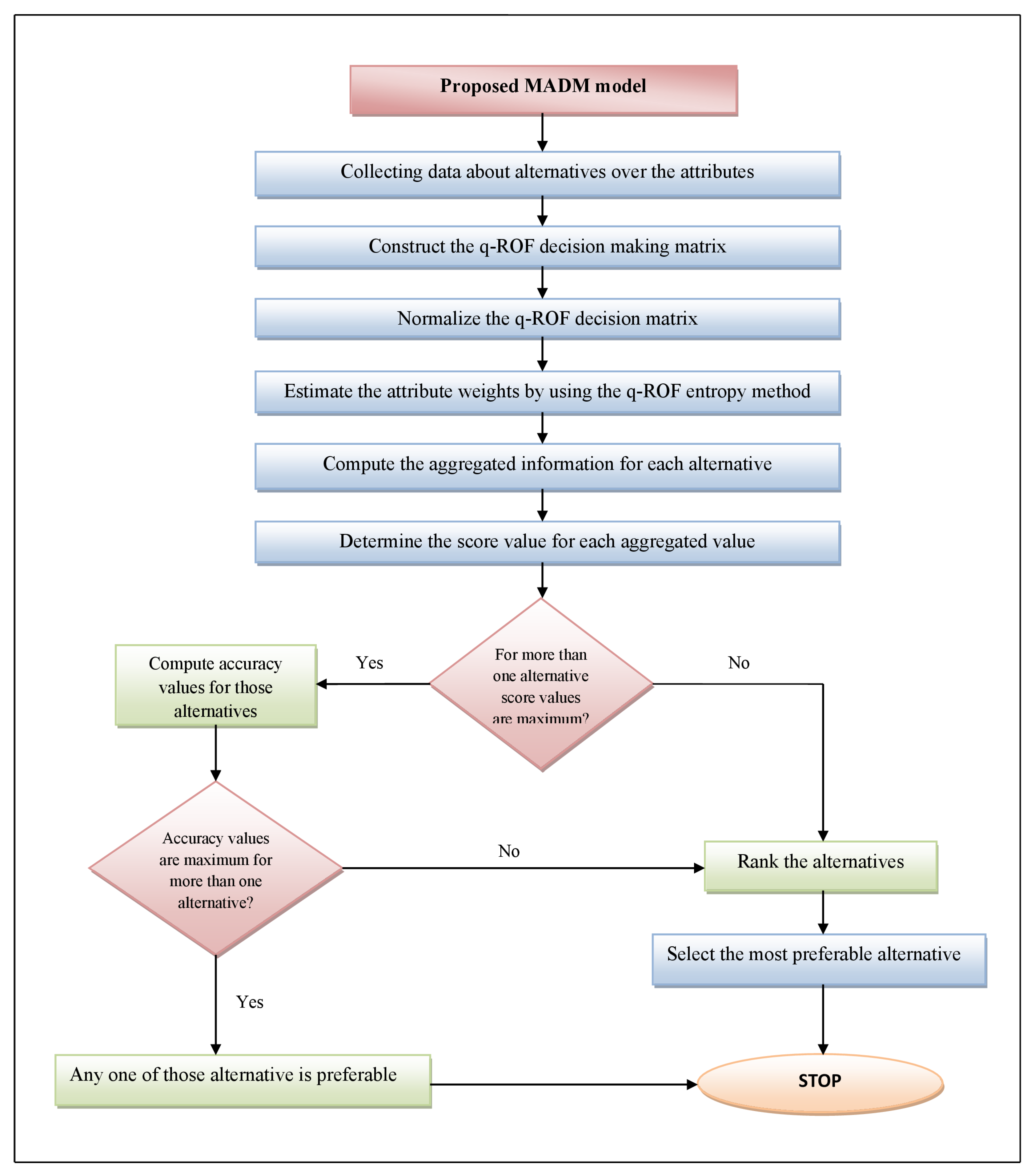
• To present a model for dealing with MADM problems that depend on the suggested q-ROFAWA and q-ROFAWG operators.
• To illustrate the potency and supremacy of the suggested model by emphasizing a numerical problem about site selection for software operating units.

The remaining portions of this article proceed as follows: several fundamental preliminaries are described in Section 2. We define a few novel operational rules for q-ROFNs based on ATCN and ATN in Section 3. In Section 4, some new AOs are established under a q-ROF environment, and their desirable characteristics are discussed based on ATCN and ATN. In Section 5, we utilize the q-ROFAWA and q-ROFAWG operators to develop some approaches for handling MADM problems. In Section 6, we elaborate on a numerical problem about site selection for software operating units to illustrate the adaptability and viability of our suggested approach. Then in Section 7, our model is compared with some well-known methods. Finally, Section 8 presents the conclusions of the paper.

2. Preliminaries

Here, we will have a look at some basic preliminaries.

Definition 1

([16]). The q-ROFS σ over the universal set P is interpreted as

$$\sigma =\{<\ell ,{\mu }_{\sigma }(\ell ),{\nu }_{\sigma }(\ell )>|\ell \in P\}.$$

Here, ${\mu }_{\sigma }:P\to [0,1]$ and ${\nu }_{\sigma }:P\to [0,1]$ are identified as the MD and the NMD to the set $\sigma$, respectively, where ${\left({\mu }_{\sigma }(\ell )\right)}^q+{\left({\nu }_{\sigma }(\ell )\right)}^q\le 1,q\ge 1$ for every $\ell \in P$. For clarity, Liu and Wang [34] defined $\sigma =({\mu }_{\sigma },{\nu }_{\sigma })$ a q-ROF number (q-ROFN).

Definition 2

([34]). The score and the accuracy functions of the q-ROFN $\sigma =({\mu }_{\sigma },{\nu }_{\sigma })$ can be illustrated as

$$\mathsf{\Phi }\left(\sigma \right)={\mu }_{\sigma }^q-{\nu }_{\sigma }^q$$

(1)

and

$$\mathsf{\Psi }\left(\sigma \right)={\mu }_{\sigma }^q+{\nu }_{\sigma }^q,$$

(2)

respectively. Here, $\mathsf{\Phi }\left(\sigma \right)\in [0,1],$ and $\mathsf{\Psi }\left(\sigma \right)\in [0,1].$

According to Definition 2, if ${\sigma }_1=({\mu }_{{\sigma }_1},{\nu }_{{\sigma }_1})$ and ${\sigma }_2=({\mu }_{{\sigma }_2},{\nu }_{{\sigma }_2})$ be any two q-ROFNs then

• ${\sigma }_1>{\sigma }_2$ if $\mathsf{\Phi }\left({\sigma }_1\right)>\mathsf{\Phi }\left({\sigma }_2\right),$
• ${\sigma }_1<{\sigma }_2$ if $\mathsf{\Phi }\left({\sigma }_1\right)<\mathsf{\Phi }\left({\sigma }_2\right),$
• If $\mathsf{\Phi }\left({\sigma }_1\right)=\mathsf{\Phi }\left({\sigma }_2\right),$ and
  • If $\mathsf{\Psi }\left({\sigma }_1\right)>\mathsf{\Psi }\left({\sigma }_2\right),$ then ${\sigma }_1>{\sigma }_2,$
  • If $\mathsf{\Psi }\left({\sigma }_1\right)=\mathsf{\Psi }\left({\sigma }_2\right),$ then ${\sigma }_1={\sigma }_2.$

ATCN and ATN

Here, we recall some basic properties of ATCN and ATN which will be utilized later.

Definition 3

([28]). Let $f,g:[0,1]\to \mathbb{R}$ be strictly decreasing and increasing continuous functions, respectively, with $f\left(1\right)=0$ and $g\left(0\right)=0$, then f and g are called decreasing generator and increasing generator, respectively.

Definition 4

([35]). With the assistance of a decreasing generator $f,$ strict ATN and strict ATCN are elicited as $T(h_1,h_2)=f^{-1}(f\left(h_1\right)+f\left(h_2\right))$ and $S(h_1,h_2)=g^{-1}(g\left(h_1\right)+g\left(h_2\right))$, respectively with $g\left(v\right)=f(1-v)$ $,\forall h_1,h_2,v\in [0,1].$

In

Table 1. Several TCN and TN with their additive generators.

Class	f	t-Norms	t-Conorms
Algebraic	$-log\left(t\right)$	$h_1{h}_2$	$h_1+h_2-h_1{h}_2$
Einstein	$log\left(\frac{2-t}{t}\right)$	$\frac{h_1{h}_2}{(1-h_1)(1-h_2)}$	$\frac{h_1+h_2}{1+h_1{h}_2}$
Hamacher ($\vartheta >0$)	$log\left(\frac{\vartheta +(1-\vartheta )t}{t}\right)$	$\frac{h_1{h}_2}{\vartheta +(1-\vartheta )(h_1+h_2-h_1{h}_2)}$	$\frac{h_1+h_2-h_1{h}_2-(1-\vartheta )h_1{h}_2}{1-(1-\vartheta )h_1{h}_2}$
Frank ($\beta >1$)	$lo{g}_{\beta }\left(\frac{\beta -1}{{\beta }^t-1}\right)$	$lo{g}_{\beta }(1+\frac{({\beta }^{h_1}-1)({\beta }^{h_2}-1)}{\beta -1})$	$lo{g}_{\beta }(1+\frac{({\beta }^{1-h_1}-1)({\beta }^{1-h_2}-1)}{\beta -1})$
Yager ($\beta >0$)	${(1-t)}^{\beta }$	$1-{({(1-h_1)}^{\beta }+{(1-h_2)}^{\beta })}^{\frac{1}{\beta }}$	${({h_1}^{\beta }+{h_2}^{\beta })}^{\frac{1}{\beta }}$

, we exhibit some renowned classes of TCN and TN as a special case of ATCN and ATN by considering different forms $f.$

3. ATCN and ATN Operations for $\mathit{q}$-ROFNs

Here, we develop a couple of fundamental set operations of q-ROFNs using ATCN and ATN.

Definition 5.

If ${\sigma }_c=({\mu }_{{\sigma }_c},{\nu }_{{\sigma }_c})(c=1,2)$ are two q-ROFNs then we have

1. 

${\sigma }_1\oplus {\sigma }_2=\left(\sqrt[q]{g^{-1}(g\left({\mu }_{{\sigma }_1}^q\right)+g\left({\mu }_{{\sigma }_2}^q\right))},\sqrt[q]{f^{-1}(f\left({\nu }_{{\sigma }_1}^q\right)+f\left({\nu }_{{\sigma }_2}^q\right))}\right).$

2. 

${\sigma }_1\otimes {\sigma }_2=\left(\sqrt[q]{f^{-1}(f\left({\mu }_{{\sigma }_1}^q\right)+f\left({\mu }_{{\sigma }_2}^q\right))},\sqrt[q]{g^{-1}(g\left({\nu }_{{\sigma }_1}^q\right)+g\left({\nu }_{{\sigma }_2}^q\right))}\right).$

3. 

$\xi {\sigma }_1=\left(\sqrt[q]{g^{-1}\left(\xi g\left({\mu }_{{\sigma }_1}^q\right)\right)},\sqrt[q]{f^{-1}\left(\xi f\left({\nu }_{{\sigma }_1}^q\right)\right)}\right),\xi >0.$

4. 

${\sigma }_1^{\xi }=\left(\sqrt[q]{f^{-1}\left(\xi f\left({\nu }_{{\sigma }_1}^q\right)\right)},\sqrt[q]{g^{-1}\left(\xi g\left({\mu }_{{\sigma }_1}^q\right)\right)}\right),\xi >0.$

Now, we define some specific relations among the operational laws in the following portion.

Proposition 1.

The following operations for two q-ROFNs${\sigma }_c=({\mu }_{{\sigma }_c},{\nu }_{{\sigma }_c})(c=1,2)$ and $\xi ,{\xi }_1,{\xi }_2>0$ are valid.

1. 

${\sigma }_1\oplus {\sigma }_2={\sigma }_2\oplus {\sigma }_1.$

2. 

${\sigma }_1\otimes {\sigma }_2={\sigma }_2\otimes {\sigma }_1.$

3. 

$\xi ({\sigma }_1\oplus {\sigma }_2)=\xi {\sigma }_1\oplus \xi {\sigma }_2.$

4. 

${\xi }_1{\sigma }_1\oplus {\xi }_2{\sigma }_1=({\xi }_1+{\xi }_2){\sigma }_1.$

5. 

${\sigma }_1^{\xi }\otimes {\sigma }_2^{\xi }={({\sigma }_1\otimes {\sigma }_2)}^{\xi }.$

6. 

${\sigma }_1^{{\xi }_1}\otimes {\sigma }_1^{{\xi }_2}={\sigma }_1^{{\xi }_1+{\xi }_2}.$

Proof. 

• ${\sigma }_1\oplus {\sigma }_2=\left(\sqrt[q]{g^{-1}(g\left({\mu }_{{\sigma }_1}^q\right)+g\left({\mu }_{{\sigma }_2}^q\right))},\sqrt[q]{f^{-1}(f\left({\nu }_{{\sigma }_1}^q\right)+f\left({\nu }_{{\sigma }_2}^q\right))}\right)$
  $=\left(\sqrt[q]{g^{-1}(g\left({\mu }_{{\sigma }_2}^q\right)+g\left({\mu }_{{\sigma }_1}^q\right))},\sqrt[q]{f^{-1}(f\left({\nu }_{{\sigma }_2}^q\right)+f\left({\nu }_{{\sigma }_1}^q\right))}\right)={\sigma }_2\oplus {\sigma }_1.$
• ${\sigma }_1\otimes {\sigma }_2=\left(\sqrt[q]{f^{-1}(f\left({\nu }_{{\sigma }_1}^q\right)+f\left({\nu }_{{\sigma }_2}^q\right))},\sqrt[q]{g^{-1}(g\left({\mu }_{{\sigma }_1}^q\right)+g\left({\mu }_{{\sigma }_2}^q\right))}\right)$
  $=\left(\sqrt[q]{f^{-1}(f\left({\nu }_{{\sigma }_2}^q\right)+f\left({\nu }_{{\sigma }_1}^q\right))},\sqrt[q]{g^{-1}(g\left({\mu }_{{\sigma }_2}^q\right)+g\left({\mu }_{{\sigma }_1}^q\right))}\right)={\sigma }_2\otimes {\sigma }_1.$
• $\xi ({\sigma }_1\oplus {\sigma }_2)=\xi \left(\sqrt[q]{g^{-1}(g\left({\mu }_{{\sigma }_1}^q\right)+g\left({\mu }_{{\sigma }_2}^q\right))},\sqrt[q]{f^{-1}(f\left({\nu }_{{\sigma }_1}^q\right)+f\left({\nu }_{{\sigma }_2}^q\right))}\right)$
  $=\left(\sqrt[q]{g^{-1}\left(\xi (g\left({\mu }_{{\sigma }_1}^q\right)+g\left({\mu }_{{\sigma }_2}^q\right))\right)},\sqrt[q]{f^{-1}\left(\xi (f\left({\nu }_{{\sigma }_1}^q\right)+f\left({\nu }_{{\sigma }_2}^q\right))\right)}\right)$
  $\xi {\sigma }_1\oplus \xi {\sigma }_2=\left(\sqrt[q]{g^{-1}\left(\xi g\left({\mu }_{{\sigma }_1}^q\right)\right)},\sqrt[q]{f^{-1}\left(\xi f\left({\nu }_{{\sigma }_1}^q\right)\right)}\right)\oplus \left(\sqrt[q]{g^{-1}\left(\xi g\left({\mu }_{{\sigma }_2}^q\right)\right)},\sqrt[q]{f^{-1}\left(\xi f\left({\nu }_{{\sigma }_2}^q\right)\right)}\right)$
  $=\left(\sqrt[q]{g^{-1}\left(\xi (g\left({\mu }_{{\sigma }_1}^q\right)+g\left({\mu }_{{\sigma }_2}^q\right))\right)},\sqrt[q]{f^{-1}\left(\xi (f\left({\nu }_{{\sigma }_1}^q\right)+f\left({\nu }_{{\sigma }_2}^q\right))\right)}\right)$
  Therefore, $\xi ({\sigma }_1\oplus {\sigma }_2)=\xi {\sigma }_1\oplus \xi {\sigma }_2.$
• ${\xi }_1{\sigma }_1\oplus {\xi }_2{\sigma }_1=\left(\sqrt[q]{g^{-1}\left({\xi }_{1}g\left({\mu }_{{\sigma }_1}^q\right)\right)},\sqrt[q]{f^{-1}\left({\xi }_{1}f\left({\nu }_{{\sigma }_1}^q\right)\right)}\right)\oplus \left(\sqrt[q]{g^{-1}\left({\xi }_{2}g\left({\mu }_{{\sigma }_1}^q\right)\right)},\sqrt[q]{f^{-1}\left({\xi }_{2}f\left({\nu }_{{\sigma }_1}^q\right)\right)}\right)$
  $=\left(\sqrt[q]{g^{-1}\left(({\xi }_1+{\xi }_2)g\left({\mu }_{{\sigma }_1}^q\right)\right)},\sqrt[q]{f^{-1}\left(({\xi }_1+{\xi }_2)f\left({\nu }_{{\sigma }_1}^q\right)\right)}\right)$
  $=({\xi }_1+{\xi }_2){\sigma }_1.$
• ${\sigma }_1^{\xi }\otimes {\sigma }_2^{\xi }=\left(\sqrt[q]{f^{-1}\left(\xi f\left({\nu }_{{\sigma }_1}^q\right)\right)},\sqrt[q]{g^{-1}\left(\xi g\left({\mu }_{{\sigma }_1}^q\right)\right)}\right)\otimes \left(\sqrt[q]{f^{-1}\left(\xi f\left({\nu }_{{\sigma }_2}^q\right)\right)},\sqrt[q]{g^{-1}\left(\xi g\left({\mu }_{{\sigma }_2}^q\right)\right)}\right)$
  $=\left(\sqrt[q]{f^{-1}\left(\xi (f\left({\mu }_{{\sigma }_1}^q\right)+f\left({\mu }_{{\sigma }_2}^q\right))\right)},\sqrt[q]{g^{-1}\left(\xi (g\left({\nu }_{{\sigma }_1}^q\right)+g\left({\nu }_{{\sigma }_2}^q\right))\right)}\right)$
  ${({\sigma }_1\otimes {\sigma }_2)}^{\xi }=\xi \left(\sqrt[q]{f^{-1}(f\left({\mu }_{{\sigma }_1}^q\right)+f\left({\mu }_{{\sigma }_2}^q\right))},\sqrt[q]{g^{-1}(g\left({\nu }_{{\sigma }_1}^q\right)+g\left({\nu }_{{\sigma }_2}^q\right))}\right)$
  $=\left(\sqrt[q]{f^{-1}\left(\xi (f\left({\mu }_{{\sigma }_1}^q\right)+f\left({\mu }_{{\sigma }_2}^q\right))\right)},\sqrt[q]{g^{-1}\left(\xi (g\left({\nu }_{{\sigma }_1}^q\right)+g\left({\nu }_{{\sigma }_2}^q\right))\right)}\right)$
  Therefore, ${\sigma }_1^{\xi }\otimes {\sigma }_2^{\xi }={({\sigma }_1\otimes {\sigma }_2)}^{\xi }.$
• ${\sigma }_1^{{\xi }_1}\otimes {\sigma }_1^{{\xi }_2}=\left(\sqrt[q]{f^{-1}\left({\xi }_{1}f\left({\nu }_{{\sigma }_1}^q\right)\right)},\sqrt[q]{g^{-1}\left({\xi }_{1}g\left({\mu }_{{\sigma }_1}^q\right)\right)}\right)\otimes \left(\sqrt[q]{f^{-1}\left({\xi }_{2}f\left({\nu }_{{\sigma }_1}^q\right)\right)},\sqrt[q]{g^{-1}\left({\xi }_{2}g\left({\mu }_{{\sigma }_1}^q\right)\right)}\right)$
  $=\left(\sqrt[q]{f^{-1}\left(({\xi }_1+{\xi }_2)f\left({\nu }_{{\sigma }_1}^q\right)\right)},\sqrt[q]{g^{-1}\left(({\xi }_1+{\xi }_2)g\left({\mu }_{{\sigma }_1}^q\right)\right)}\right)$
  $={\sigma }_1^{{\xi }_1+{\xi }_2}.$

□

Proposition 2.

Let $h_1={\sigma }_1\oplus {\sigma }_2,$ $h_2={\sigma }_1\otimes {\sigma }_2,$ $h_3=\xi {\sigma }_1,$ $h_4={\left({\sigma }_1\right)}^{\xi }$ for two q-ROFNs${\sigma }_c=({\mu }_{{\sigma }_c},{\nu }_{{\sigma }_c})(c=1,2)$ where $\xi (\in \mathbb{R})>0.$ Then $h_1,h_2,h_3$ and $h_4$ are also q-ROFNs.

Proof. 

Since $g\left(v\right)=f(1-v)$, and $f:[0,1]\to [0,\infty ]$ is a strictly decreasing function, then $g\left(v\right)$ is a strictly increasing function, which implies that $0\le f^{-1}(f\left({\mu }_{{\sigma }_1}\right)+f\left({\mu }_{{\sigma }_2}\right))\le 1$ and $0\le g^{-1}(g\left({\mu }_{{\sigma }_1}\right)+g\left({\mu }_{{\sigma }_2}\right))\le 1.$ Additionally,

$$\begin{array}{c}{\left(\sqrt[q]{g^{-1}(g\left({\mu }_{{\sigma }_1}^q\right)+g\left({\mu }_{{\sigma }_2}^q\right))}\right)}^q+{\left(\sqrt[q]{f^{-1}(f\left({\nu }_{{\sigma }_1}^q\right)+f\left({\nu }_{{\sigma }_2}^q\right))}\right)}^q\hfill \\ =\left(g^{-1}(g\left({\mu }_{{\sigma }_1}^q\right)+g\left({\mu }_{{\sigma }_2}^q\right))\right)+\left(f^{-1}(f\left({\nu }_{{\sigma }_1}^q\right)+f\left({\nu }_{{\sigma }_2}^q\right))\right)\hfill \\ \le \left(f^{-1}(f\left({\nu }_{{\sigma }_1}^q\right)+f\left({\nu }_{{\sigma }_2}^q\right))\right)+\left(g^{-1}(g(1-{\nu }_{{\sigma }_1}^q)+g(1-{\nu }_{{\sigma }_2}^q))\right)[\because {\mu }_{{\sigma }_i}^q\le 1-{\nu }_{{\sigma }_i}^q]\hfill \\ =\left(f^{-1}(f\left({\nu }_{{\sigma }_1}^q\right)+f\left({\nu }_{{\sigma }_2}^q\right))\right)+\left(g^{-1}(f\left({\nu }_{{\sigma }_1}^q\right)+f\left({\nu }_{{\sigma }_2}^q\right))\right)[\because g\left(v\right)=f(1-v)]\hfill \\ =f^{-1}(f\left({\nu }_{{\sigma }_1}^q\right)+f\left({\nu }_{{\sigma }_2}^q\right))+1-f^{-1}(f\left({\nu }_{{\sigma }_1}^q\right)+f\left({\nu }_{{\sigma }_2}^q\right))[\because g^{-1}\left(v\right)=1-f^{-1}\left(v\right)]\hfill \\ =1.\hfill \end{array}$$

Therefore, $h_1={\sigma }_1\oplus {\sigma }_2$ and $h_2={\sigma }_1\otimes {\sigma }_2$ are q-ROFNs.

Proceeding similarly we obtain $h_3=\xi {\sigma }_1$ and $h_4={\left({\sigma }_1\right)}^{\xi }$ which are also q-ROFNs. □

4. ATCN and ATN Based $\mathit{q}$-ROF AOs

Here, we develop the q-ROFAWA, q-ROFAOWA, q-ROFAHA, q-ROFAWG, q-ROFAOWG and q-ROFAHG AOs based on ATCN and ATN to aggregate q-ROF information.

4.1. q-ROFAWA and q-ROFAWG Operators

Definition 6.

Let ${\sigma }_c=({\mu }_{{\sigma }_c},{\nu }_{{\sigma }_c})(c=1\left(1\right)u)$ be the q-ROFNs with their associated weight vector $\delta ={({\delta }_1,{\delta }_2,\cdots ,{\delta }_u)}^T,$ where ${\delta }_c\in [0,1]$ and ${\displaystyle \sum _{c=1}^u}{\delta }_c=1.$ Based on ATCN and ATN the q-ROFAWA operator and q-ROFAWG operator are mappings from ${\sigma }^u$ to σ and are given by

$$q\text{-ROFAWA}({\sigma }_1,{\sigma }_2,\cdots ,{\sigma }_u)={\displaystyle \underset{c=1}{\overset{u}{⨁}}}{\delta }_c{\sigma }_c$$

and

$$q\text{-ROFAWG}({\sigma }_1,{\sigma }_2,\cdots ,{\sigma }_u)={\displaystyle \underset{c=1}{\overset{u}{⨂}}}{\delta }_c{\sigma }_c,$$

respectively.

Theorem 1.

The aggregated result of the q-ROFNs ${\sigma }_c=({\mu }_{{\sigma }_c},{\nu }_{{\sigma }_c})(c=1\left(1\right)u)$ using q-ROFAWA and q-ROFAWG operators are also q-ROFNs and are defined as follows

$$q\text{-ROFAWA}({\sigma }_1,{\sigma }_2,\cdots ,{\sigma }_u)={\displaystyle \underset{c=1}{\overset{u}{⨁}}}{\delta }_c{\sigma }_c=\left(\sqrt[q]{g^{-1}\left({\displaystyle \sum _{c=1}^u}{\delta }_{c}g\left({\mu }_{{\sigma }_c}^q\right)\right)},\sqrt[q]{f^{-1}\left({\displaystyle \sum _{c=1}^u}{\delta }_{c}f\left({\nu }_{{\sigma }_c}^q\right)\right)}\right)$$

(3)

and

$$q\text{-ROFAWG}({\sigma }_1,{\sigma }_2,\cdots ,{\sigma }_u)={\displaystyle \underset{c=1}{\overset{u}{⨂}}}{\delta }_c{\sigma }_c=\left(\sqrt[q]{f^{-1}\left({\displaystyle \sum _{c=1}^u}{\delta }_{c}f\left({\mu }_{{\sigma }_c}^q\right)\right)},\sqrt[q]{g^{-1}\left({\displaystyle \sum _{c=1}^u}{\delta }_{c}g\left({\nu }_{{\sigma }_c}^q\right)\right)}\right).$$

(4)

Here, f is an additive generator of continuous ATN.

Proof. 

We have established the above theorem by applying the mathematical induction principle.

For two q-ROFNs ${\sigma }_1$ and ${\sigma }_2$, we obtain

$$\begin{array}{c}q\text{-ROFAWA}({\sigma }_1,{\sigma }_2)={\displaystyle \underset{c=1}{\overset{2}{⨁}}}{\delta }_c{\sigma }_c={\delta }_1{\sigma }_1⨁{\delta }_2{\sigma }_2\hfill \\ =\left(\sqrt[q]{g^{-1}\left({\delta }_{1}g\left({\mu }_{{\sigma }_1}^q\right)\right)},\sqrt[q]{f^{-1}\left({\delta }_{1}f\left({\nu }_{{\sigma }_1}^q\right)\right)}\right)⨁\left(\sqrt[q]{g^{-1}\left({\delta }_{2}g\left({\mu }_{{\sigma }_2}^q\right)\right)},\sqrt[q]{f^{-1}\left({\delta }_{2}f\left({\nu }_{{\sigma }_2}^q\right)\right)}\right)\hfill \\ =\left(\sqrt[q]{g^{-1}\left({\displaystyle \sum _{c=1}^2}{\delta }_{c}g\left({\mu }_{{\sigma }_c}^q\right)\right)},\sqrt[q]{f^{-1}\left({\displaystyle \sum _{c=1}^2}{\delta }_{c}f\left({\nu }_{{\sigma }_c}^q\right)\right)}\right).\hfill \end{array}$$

As a result, the outcome exists for $u=2.$

We presume that the outcome is effective when $u=x.$

Therefore $q\text{-ROFAWA}({\sigma }_1,{\sigma }_2,\cdots ,{\sigma }_x)=\left(\sqrt[q]{g^{-1}\left({\displaystyle \sum _{c=1}^x}{\delta }_{c}g\left({\mu }_{{\sigma }_c}^q\right)\right)},\sqrt[q]{f^{-1}\left({\displaystyle \sum _{c=1}^x}{\delta }_{c}f\left({\nu }_{{\sigma }_c}^q\right)\right)}\right).$

Now, $q\text{-ROFAWA}{\sigma }_1,{\sigma }_2,\cdots ,{\sigma }_x,{\sigma }_{x+1})$=${\displaystyle \underset{c=1}{\overset{x+1}{⨁}}}{\delta }_c{\sigma }_c$=${\displaystyle \underset{c=1}{\overset{x}{⨁}}}{\delta }_c{\sigma }_c⨁{\delta }_{x+1}{\sigma }_{x+1}$

$=\left(\sqrt[q]{g^{-1}\left({\displaystyle \sum _{c=1}^x}{\delta }_{c}g\left({\mu }_{{\sigma }_c}^q\right)\right)},\sqrt[q]{f^{-1}\left({\displaystyle \sum _{c=1}^x}{\delta }_{c}f\left({\nu }_{{\sigma }_c}^q\right)\right)}\right)$$⨁\left(\sqrt[q]{g^{-1}\left({\delta }_{x+1}g\left({\mu }_{{\sigma }_{x+1}}^q\right)\right)},\sqrt[q]{f^{-1}\left({\delta }_{x+1}f\left({\nu }_{{\sigma }_{x+1}}^q\right)\right)}\right)$

$=\left(\sqrt[q]{g^{-1}\left({\displaystyle \sum _{c=1}^{x+1}}{\delta }_{c}g\left({\mu }_{{\sigma }_c}^q\right)\right)},\sqrt[q]{f^{-1}\left({\displaystyle \sum _{c=1}^{x+1}}{\delta }_{c}f\left({\nu }_{{\sigma }_c}^q\right)\right)}\right).$

As a result, the result is valid when $u=x+1.$

Hence, the outcome is effective for all natural numbers $u.$ □

The other part of this theorem can be proved similarly.

Next, we show that our proposed q-ROFAWA and q-ROFAWG operators met the subsequent characteristics:

Theorem 2.

(Idempotency property). If the collection of q-ROFNs ${\sigma }_c=({\mu }_{{\sigma }_c},{\nu }_{{\sigma }_c})(c=1\left(1\right)u)$ are equal, i.e., if ${\sigma }_c=\sigma =({\mu }_{\sigma },{\nu }_{\sigma }),\forall c,$ then

$q\text{-ROFAWA}({\sigma }_1,{\sigma }_2,\cdots ,{\sigma }_u)=\sigma$ and $q\text{-ROFAWG}({\sigma }_1,{\sigma }_2,\cdots ,{\sigma }_u)=\sigma .$

Proof. 

Let ${\sigma }_c=\sigma ,\forall c=1,2\cdots u.$ Then ${\mu }_{{\sigma }_c}={\mu }_{\sigma }$ and ${\nu }_{{\sigma }_c}={\nu }_{\sigma },\forall c=1\left(1\right)u.$

$$\begin{array}{c}q\text{-ROFAWA}({\sigma }_1,{\sigma }_2,\cdots ,{\sigma }_u)=\left(\sqrt[q]{g^{-1}\left({\displaystyle \sum _{c=1}^u}{\delta }_{c}g\left({\mu }_{{\sigma }_c}^q\right)\right)},\sqrt[q]{f^{-1}\left({\displaystyle \sum _{c=1}^u}{\delta }_{c}f\left({\nu }_{{\sigma }_c}^q\right)\right)}\right)\hfill \\ =\left(\sqrt[q]{g^{-1}\left({\displaystyle \sum _{c=1}^u}{\delta }_{c}g\left({\mu }_{\sigma }^q\right)\right)},\sqrt[q]{f^{-1}\left({\displaystyle \sum _{c=1}^u}{\delta }_{c}f\left({\nu }_{\sigma }^q\right)\right)}\right)\hfill \\ =\left(\sqrt[q]{g^{-1}\left(g\left({\mu }_{\sigma }^q\right)\right)},\sqrt[q]{f^{-1}\left(f\left({\nu }_{\sigma }^q\right)\right)}\right)=({\mu }_{\sigma },{\nu }_{\sigma })=\sigma .\hfill \end{array}$$

□

The other part can be proven in a similar manner.

Theorem 3.

(Monotonicity property). Let $\{{\sigma }_1,{\sigma }_2,\cdots ,{\sigma }_u\}$ and $\{{\widehat{\sigma }}_1,{\widehat{\sigma }}_2,\cdots ,{\widehat{\sigma }}_u\}$ be two sets of q-ROFNs, where ${\sigma }_c=({\mu }_{{\sigma }_c},{\nu }_{{\sigma }_c})$ and ${\widehat{\sigma }}_c=({\mu }_{{\widehat{\sigma }}_c},{\nu }_{{\widehat{\sigma }}_c})$ for $c=1,2,\cdots ,u.$ If ${\mu }_{{\sigma }_c}\le {\mu }_{{\widehat{\sigma }}_c}$ and ${\nu }_{{\sigma }_c}\ge {\nu }_{{\widehat{\sigma }}_c}$ for all c, then, q-ROFAWA$({\sigma }_1,{\sigma }_2,\cdots ,{\sigma }_u)\le$ q-ROFAWA$({\widehat{\sigma }}_1,{\widehat{\sigma }}_2,\cdots ,{\widehat{\sigma }}_u)$ and q-ROFAWG$({\sigma }_1,{\sigma }_2,\cdots ,{\sigma }_u)\le$ q-ROFAWG$({\widehat{\sigma }}_1,{\widehat{\sigma }}_2,\cdots ,{\widehat{\sigma }}_u).$

Proof. 

Since ${\mu }_{{\sigma }_c}\le {\mu }_{{\widehat{\sigma }}_c}$ and ${\nu }_{{\sigma }_c}\ge {\nu }_{{\widehat{\sigma }}_c}$ for all $c=1,2,\cdots ,u$, then, ${\mu }_{{\sigma }_c}\le {\mu }_{{\widehat{\sigma }}_c}\Rightarrow {\mu }_{{\sigma }_c}^q$ $\le {\mu }_{{\widehat{\sigma }}_c}^q\Rightarrow g\left({\mu }_{{\sigma }_c}^q\right)\le g\left({\mu }_{{\widehat{\sigma }}_c}^q\right)\Rightarrow {\delta }_{c}g\left({\mu }_{{\sigma }_c}^q\right)\le {\delta }_{c}g\left({\mu }_{{\widehat{\sigma }}_c}^q\right)\Rightarrow {\displaystyle \sum _{c=1}^u}{\delta }_{c}g\left({\mu }_{{\sigma }_c}^q\right)\le {\displaystyle \sum _{c=1}^u}{\delta }_{c}g\left({\mu }_{{\widehat{\sigma }}_c}^q\right)\Rightarrow \sqrt[q]{g^{-1}\left({\displaystyle \sum _{c=1}^u}{\delta }_{c}g\left({\mu }_{{\sigma }_c}^q\right)\right)}\le \sqrt[q]{g^{-1}\left({\displaystyle \sum _{c=1}^u}{\delta }_{c}g\left({\mu }_{{\widehat{\sigma }}_c}^q\right)\right)}.$

Similarly, it can be shown that $\sqrt[q]{f^{-1}\left({\displaystyle \sum _{c=1}^u}{\delta }_{c}f\left({\nu }_{{\sigma }_c}^q\right)\right)}\ge \sqrt[q]{f^{-1}\left({\displaystyle \sum _{c=1}^u}{\delta }_{c}f\left({\nu }_{{\widehat{\sigma }}_c}^q\right)\right)}.$

Thus,

$$\begin{array}{c}{\left(\sqrt[q]{g^{-1}\left({\displaystyle \sum _{c=1}^u}{\delta }_{c}g\left({\mu }_{{\sigma }_c}^q\right)\right)}\right)}^q-{\left(\sqrt[q]{f^{-1}\left({\displaystyle \sum _{c=1}^u}{\delta }_{c}f\left({\nu }_{{\sigma }_c}^q\right)\right)}\right)}^q\le \hfill \\ {\left(\sqrt[q]{g^{-1}\left({\displaystyle \sum _{c=1}^u}{\delta }_{c}g\left({\mu }_{{\widehat{\sigma }}_c}^q\right)\right)}\right)}^q-{\left(\sqrt[q]{f^{-1}\left({\displaystyle \sum _{c=1}^u}{\delta }_{c}f\left({\nu }_{{\widehat{\sigma }}_c}^q\right)\right)}\right)}^q.\hfill \end{array}$$

Let $\sigma =q\text{-ROFAWA}({\sigma }_1,{\sigma }_2,\cdots ,{\sigma }_u)$ and $\widehat{\sigma }=q\text{-ROFAWA}({\widehat{\sigma }}_1^{\prime },{\widehat{\sigma }}_2^{\prime },\cdots ,{\widehat{\sigma }}_u^{\prime }).$ Then by Definition 2, we have, $\mathsf{\Phi }\left(\sigma \right)\le \mathsf{\Phi }\left(\widehat{\sigma }\right).$

(I)

If $\mathsf{\Phi }\left(\sigma \right)<\mathsf{\Phi }\left(\widehat{\sigma }\right)$ then we have,

$\sigma <\widehat{\sigma }$ i.e., $q\text{-ROFAWA}({\sigma }_1,{\sigma }_2,\cdots ,{\sigma }_u)<q\text{-ROFAWA}({\sigma }_1^{\prime },{\sigma }_2^{\prime },\cdots ,{\sigma }_u^{\prime }).$

(II)

If $\mathsf{\Phi }\left(\sigma \right)=\mathsf{\Phi }\left(\widehat{\sigma }\right)$ then, we obtain

${\left(\sqrt[q]{g^{-1}\left({\displaystyle \sum _{c=1}^u}{\delta }_{c}g\left({\mu }_{{\sigma }_c}^q\right)\right)}\right)}^q-{\left(\sqrt[q]{f^{-1}\left({\displaystyle \sum _{c=1}^u}{\delta }_{c}f\left({\nu }_{{\sigma }_c}^q\right)\right)}\right)}^q={\left(\sqrt[q]{g^{-1}\left({\displaystyle \sum _{c=1}^u}{\delta }_{c}g\left({\mu }_{{\widehat{\sigma }}_c}^q\right)\right)}\right)}^q-{\left(\sqrt[q]{f^{-1}\left({\displaystyle \sum _{c=1}^u}{\delta }_{c}f\left({\nu }_{{\widehat{\sigma }}_c}^q\right)\right)}\right)}^q,$

then, by the condition ${\mu }_{{\sigma }_c}\le {\mu }_{{\widehat{\sigma }}_c}$ and ${\nu }_{{\sigma }_c}\ge {\nu }_{{\widehat{\sigma }}_c}$ for all $c=1\left(1\right)u$, we have

${\left(\sqrt[q]{g^{-1}\left({\displaystyle \sum _{c=1}^u}{\delta }_{c}g\left({\mu }_{{\sigma }_c}^q\right)\right)}\right)}^q={\left(\sqrt[q]{g^{-1}\left({\displaystyle \sum _{c=1}^u}{\delta }_{c}g\left({\mu }_{{\widehat{\sigma }}_c}^q\right)\right)}\right)}^q$ and

${\left(\sqrt[q]{f^{-1}\left({\displaystyle \sum _{c=1}^u}{\delta }_{c}f\left({\nu }_{{\sigma }_c}^q\right)\right)}\right)}^q={\left(\sqrt[q]{f^{-1}\left({\displaystyle \sum _{c=1}^u}{\delta }_{c}f\left({\nu }_{{\widehat{\sigma }}_c}^q\right)\right)}\right)}^q.$

So, from Definition 2, we have

$\mathsf{\Psi }\left(\sigma \right)={\left(\sqrt[q]{g^{-1}\left({\displaystyle \sum _{c=1}^u}{\delta }_{c}g\left({\mu }_{{\sigma }_c}^q\right)\right)}\right)}^q+{\left(\sqrt[q]{f^{-1}\left({\displaystyle \sum _{c=1}^u}{\delta }_{c}f\left({\nu }_{{\sigma }_c}^q\right)\right)}\right)}^q$

$={\left(\sqrt[q]{g^{-1}\left({\displaystyle \sum _{c=1}^u}{\delta }_{c}g\left({\mu }_{{\widehat{\sigma }}_c}^q\right)\right)}\right)}^q+{\left(\sqrt[q]{f^{-1}\left({\displaystyle \sum _{c=1}^u}{\delta }_{c}f\left({\nu }_{{\widehat{\sigma }}_c}^q\right)\right)}\right)}^q=\mathsf{\Psi }\left(\widehat{\sigma }\right).$

Therefore, from (I) and (II), $q\text{-ROFAWA}({\sigma }_1,{\sigma }_2,\cdots ,{\sigma }_u)\le q\text{-ROFAWA}({\widehat{\sigma }}_1,{\widehat{\sigma }}_2,\cdots ,{\widehat{\sigma }}_u).$ □

The other part can be proven in a similar fashion.

Theorem 4.

(Boundedness property). For a number of q-ROFNs ${\sigma }_c=({\mu }_{{\sigma }_c},{\nu }_{{\sigma }_c})(c=1,2,\cdots ,u),$ let ${\sigma }^{-}=(\underset{c}{min}{\mu }_{{\sigma }_c},\underset{c}{max}{\nu }_{{\sigma }_c}),$ ${\sigma }^{+}=(\underset{c}{max}{\mu }_{{\sigma }_c},\underset{c}{min}{\nu }_{{\sigma }_c}).$ Then

${\sigma }^{-}\le q\text{-ROFAWA}({\sigma }_1,{\sigma }_2,\cdots ,{\sigma }_u)\le {\sigma }^{+}$ and ${\sigma }^{-}\le q\text{-ROFAWG}({\sigma }_1,{\sigma }_2,\cdots ,{\sigma }_u)\le {\sigma }^{+}.$

Proof. 

For every $c(c=1,2,\cdots ,u),$ we have $\underset{c}{min}{\mu }_{{\sigma }_c}\le {\mu }_{{\sigma }_c}\le \underset{c}{max}{\mu }_{{\sigma }_c} \mathrm{and} \underset{c}{min}{\nu }_{{\sigma }_c}\le {\nu }_{{\sigma }_c}\le \underset{c}{max}{\nu }_{{\sigma }_c}$ which implies that

$\sqrt[q]{g^{-1}\left({\displaystyle \sum _{c=1}^u}{\delta }_{c}g\left({\left(\underset{c}{min}{\mu }_{{\sigma }_c}\right)}^q\right)\right)}\le \sqrt[q]{g^{-1}\left({\displaystyle \sum _{c=1}^u}{\delta }_{c}g\left({\mu }_{{\sigma }_c}^q\right)\right)}\le \sqrt[q]{g^{-1}\left({\displaystyle \sum _{c=1}^u}{\delta }_{c}g\left({\left(\underset{c}{max}{\mu }_{{\sigma }_c}\right)}^q\right)\right)}$ and $\sqrt[q]{f^{-1}\left({\displaystyle \sum _{c=1}^u}{\delta }_{c}f\left({\left(\underset{c}{min}{\mu }_{{\sigma }_c}\right)}^q\right)\right)}\le \sqrt[q]{f^{-1}\left({\displaystyle \sum _{c=1}^u}{\delta }_{c}f\left({\mu }_{{\sigma }_c}^q\right)\right)}\le \sqrt[q]{f^{-1}\left({\displaystyle \sum _{c=1}^u}{\delta }_{c}f\left({\left(\underset{c}{max}{\mu }_{{\sigma }_c}\right)}^q\right)\right)}.$

Therefore, ${\sigma }^{-}\le q\text{-ROFAWA}({\sigma }_1,{\sigma }_2,\cdots ,{\sigma }_u)\le {\sigma }^{+}.$ □

The rest of the theorem can be proved similarly.

Deduction 1.

If we assign different forms of the additive generator $f,$ then we obtain some particular forms of $q\text{-ROFAWA}$ and $q\text{-ROFAWG}$ operators.

Table 2. Some particular forms of $q\text{-ROFAWA}$ and $q\text{-ROFAWG}$ operators for different f.

f	Classes of t-Norm and t-Conorm	Weighted Averaging (WA)/ Weighted Geometric (WG)	q-ROF Aggregation Operator	Aggregating Value of a Collection of q-ROFNs ${\mathit{\sigma }}_1,{\mathit{\sigma }}_2,\cdots ,{\mathit{\sigma }}_{\mathit{u}}$
$log\left(t\right)$	Algebric Class	WA	Weighted averaging operator (q-ROFWA) [34]	$\left(\sqrt[q]{1-{\displaystyle \prod _{c=1}^u}{(1-{\mu }_{{\sigma }_c}^q)}^{{\delta }_c}},{\displaystyle \prod _{c=1}^u}{\nu }_{{\sigma }_c}^{{\delta }_c}\right)$
		WG	Weighted geometric operator (q-ROFWG) [34]	$\left({\displaystyle \prod _{c=1}^u}{\mu }_{{\sigma }_c}^{{\delta }_c},\sqrt[q]{1-{\displaystyle \prod _{c=1}^u}{(1-{\nu }_{{\sigma }_c}^q)}^{{\delta }_c}}\right)$
$log\frac{2-t}{t}$	Einstein Class	WA	Einstein weighted averaging operator (q-ROFEWA) [36]	$\left(\sqrt[q]{\frac{{\displaystyle \prod _{c=1}^u}{(1+{\mu }_{{\sigma }_c}^q)}^{{\delta }_c}-{\displaystyle \prod _{c=1}^u}{(1-{\mu }_{{\sigma }_c}^q)}^{{\delta }_c}}{{\displaystyle \prod _{c=1}^u}{(1+{\mu }_{{\sigma }_c}^q)}^{{\delta }_c}+{\displaystyle \prod _{c=1}^u}{(1-{\mu }_{{\sigma }_c}^q)}^{{\delta }_c}}},\frac{\sqrt[q]{2}{\displaystyle \prod _{c=1}^u}{\nu }_{{\sigma }_c}^{{\delta }_c}}{\sqrt[q]{{\displaystyle \prod _{c=1}^u}{(2-{\nu }_{{\sigma }_c}^q)}^{{\delta }_c}+{\displaystyle \prod _{c=1}^u}{\left({\nu }_{{\sigma }_c}^q\right)}^{{\delta }_c}}}\right)$
		WG	Einstein weighted geometric operator (q-ROFEWG) [36]	$\left(\frac{\sqrt[q]{2}{\displaystyle \prod _{c=1}^u}{\mu }_{{\sigma }_c}^{{\delta }_c}}{\sqrt[q]{{\displaystyle \prod _{c=1}^u}{(2-{\mu }_{{\sigma }_c}^q)}^{{\delta }_c}+{\displaystyle \prod _{c=1}^u}{\left({\mu }_{{\sigma }_c}^q\right)}^{{\delta }_c}}},\sqrt[q]{\frac{{\displaystyle \prod _{c=1}^u}{(1+{\nu }_{{\sigma }_c}^q)}^{{\delta }_c}-{\displaystyle \prod _{c=1}^u}{(1-{\nu }_{{\sigma }_c}^q)}^{{\delta }_c}}{{\displaystyle \prod _{c=1}^u}{(1+{\nu }_{{\sigma }_c}^q)}^{{\delta }_c}+{\displaystyle \prod _{c=1}^u}{(1-{\nu }_{{\sigma }_c}^q)}^{{\delta }_c}}}\right).$
$log\left(\frac{\vartheta +(1-\vartheta )t}{t}\right)$	Hamacher Class	WA	Hamacher weighted averaging operator (q-ROFHWG) [36]	$\left(\sqrt[q]{\frac{{\displaystyle \prod _{c=1}^u}{(1+(\vartheta -1){\mu }_{{\sigma }_c}^q)}^{{\delta }_c}-{\displaystyle \prod _{c=1}^u}{(1-{\mu }_{{\sigma }_c}^q)}^{{\delta }_c}}{{\displaystyle \prod _{c=1}^u}{(1+(\vartheta -1){\mu }_{{\sigma }_c}^q)}^{{\delta }_c}+(\vartheta -1){\displaystyle \prod _{c=1}^u}{(1-{\mu }_{{\sigma }_c}^q)}^{{\delta }_c}}},\frac{\sqrt[q]{\vartheta }{\displaystyle \prod _{c=1}^u}{\nu }_{{\sigma }_c}^{{\delta }_c}}{\sqrt[q]{{\displaystyle \prod _{c=1}^u}{[1+(\vartheta -1)(1-{\nu }_{{\sigma }_c}^q)]}^{{\delta }_c}+(\vartheta -1){\displaystyle \prod _{c=1}^u}{\left({\nu }_{{\sigma }_c}^q\right)}^{{\delta }_c}}}\right)$
		WG	Hamacher weighted geometric operator (q-ROFHWG) [36]	$\left(\frac{\sqrt[q]{\vartheta }{\displaystyle \prod _{c=1}^u}{\mu }_{{\sigma }_c}^{{\delta }_c}}{\sqrt[q]{{\displaystyle \prod _{c=1}^u}{[1+(\vartheta -1)(1-{\mu }_{{\sigma }_c}^q)]}^{{\delta }_c}+(\vartheta -1){\displaystyle \prod _{c=1}^u}{\left({\mu }_{{\sigma }_c}^q\right)}^{{\delta }_c}}},\sqrt[q]{\frac{{\displaystyle \prod _{c=1}^u}{(1+(\vartheta -1){\nu }_{{\sigma }_c}^q)}^{{\delta }_c}-{\displaystyle \prod _{c=1}^u}{(1-{\nu }_{{\sigma }_c}^q)}^{{\delta }_c}}{{\displaystyle \prod _{c=1}^u}{(1+(\vartheta -1){\nu }_{{\sigma }_c}^q)}^{{\delta }_c}+(\vartheta -1){\displaystyle \prod _{c=1}^u}{(1-{\nu }_{{\sigma }_c}^q)}^{{\delta }_c}}}\right)$
$log\frac{\beta -1}{{\beta }^t-1}$	Frank Class	WA	Frank weighted averaging operator (q-ROFFWA)	$\left(\sqrt[q]{1-{log}_{\beta }\left(1+{\displaystyle \prod _{c=1}^k}{({\beta }^{1-{\mu }_{{\sigma }_c}^q}-1)}^{{\delta }_c}\right)},\sqrt[q]{{log}_{\beta }\left(1+{\displaystyle \prod _{c=1}^k}{({\beta }^{{\nu }_{{\sigma }_c}^q}-1)}^{{\delta }_c}\right)}\right)$
		WG	Frank weighted geometric operator (q-ROFFWG)	$\left(\sqrt[q]{{log}_{\beta }\left(1+{\displaystyle \prod _{c=1}^k}{({\beta }^{{\mu }_{{\sigma }_c}^q}-1)}^{{\delta }_c}\right)},\sqrt[q]{1-{log}_{\beta }\left(1+{\displaystyle \prod _{c=1}^k}{({\beta }^{1-{\nu }_{{\sigma }_c}^q}-1)}^{{\delta }_c}\right)}\right)$
${(1-t)}^{\beta },\beta >0$	Yager Class	WA	Yager weighted averaging operator (Yq-ROFWA)	$\left({\left({\displaystyle \sum _{c=1}^u}{\delta }_c{\left({\mu }_{{\sigma }_c}^q\right)}^{\beta }\right)}^{\frac{1}{\beta }},1-{\left({\displaystyle \sum _{c=1}^u}{\delta }_c{(1-{\nu }_{{\sigma }_c}^q)}^{\beta }\right)}^{\frac{1}{\beta }}\right)$
		WG	Yager weighted geometric operator operator (Yq-ROFWG)	$\left(1-{\left({\displaystyle \sum _{c=1}^u}{\delta }_c{(1-{\mu }_{{\sigma }_c}^q)}^{\beta }\right)}^{\frac{1}{\beta }},{\left({\displaystyle \sum _{c=1}^u}{\delta }_c{\left({\nu }_{{\sigma }_c}^q\right)}^{\beta }\right)}^{\frac{1}{\beta }}\right)$

illustrates these particular forms of $f.$

Deduction 2.

If we put different values for the parameter $q,$ we obtain the following cases:

1. 

For $q=1$ the q-ROFAWA and q-ROFAWG operators are transformed into intuitionistic fuzzy Archimedian weighted averaging (IFAWA) [37] and IF Archimedian weighted geometric (IFAWG) [37] operators, respectively. Therefore

$IFAWA({\sigma }_1,{\sigma }_2,\cdots ,{\sigma }_u)={\displaystyle \underset{c=1}{\overset{u}{⨁}}}{\delta }_c{\sigma }_c=\left(g^{-1}\left({\displaystyle \sum _{c=1}^u}{\delta }_{c}g\left({\mu }_{{\sigma }_c}\right)\right),f^{-1}\left({\displaystyle \sum _{c=1}^u}{\delta }_{c}f\left({\nu }_{{\sigma }_c}\right)\right)\right)$

$IFAWG({\sigma }_1,{\sigma }_2,\cdots ,{\sigma }_u)={\displaystyle \underset{c=1}{\overset{u}{⨂}}}{\delta }_c{\sigma }_c=\left(f^{-1}\left({\displaystyle \sum _{c=1}^u}{\delta }_{c}f\left({\mu }_{{\sigma }_c}\right)\right),g^{-1}\left({\displaystyle \sum _{c=1}^u}{\delta }_{c}g\left({\nu }_{{\sigma }_c}\right)\right)\right).$

Remark 1.

For the different form of the additive generator $f,$ we obtain some special cases of IFAWA and IFAWG operators. For example, If $f\left(t\right)=-log\left(t\right),$ IFAWA and IFAWG operators are transformed into intuitionistic fuzzy weighted averaging (IFWA) [38] and intuitionistic fuzzy weighted geometric (IFWG) [39] operators, respectively. If $f\left(t\right)=-log\left(\frac{2-t}{t}\right),$ IFAWA and IFAWAoperators are transformed into Einstein intuitionistic fuzzy weighted averaging (EIFWA) [37,40] and Einstein intuitionistic fuzzy weighted geometric (EIFWG) [41] operators, respectively, etc.

2. 

If $q=2,$ then q-ROFAWA and q-ROFAWG operators are transformed into Pythagorean fuzzy Archimedian weighted averaging (PFAWA) operators and Pythagorean fuzzy Archimedian weighted geometric (PFAWG) operators, respectively, and they are given by

$PFAWA({\sigma }_1,{\sigma }_2,\cdots ,{\sigma }_u)={\displaystyle \underset{c=1}{\overset{u}{⨁}}}{\delta }_c{\sigma }_c=\left(\sqrt{g^{-1}\left({\displaystyle \sum _{c=1}^u}{\delta }_{c}g\left({\mu }_{{\sigma }_c}^2\right)\right)},\sqrt{f^{-1}\left({\displaystyle \sum _{c=1}^u}{\delta }_{c}f\left({\nu }_{{\sigma }_c}^2\right)\right)}\right)$

$PFAWG({\sigma }_1,{\sigma }_2,\cdots ,{\sigma }_u)={\displaystyle \underset{c=1}{\overset{u}{⨂}}}{\delta }_c{\sigma }_c=\left(\sqrt{f^{-1}\left({\displaystyle \sum _{c=1}^u}{\delta }_{c}f\left({\mu }_{{\sigma }_c}^2\right)\right)},\sqrt{g^{-1}\left({\displaystyle \sum _{c=1}^u}{\delta }_{c}g\left({\nu }_{{\sigma }_c}^2\right)\right)}\right),$

respectively.

Remark 2.

If the additive generator f is taken in different forms, then we obtain some special cases of PFAWA operator. For example, If $f\left(t\right)=-log\left(t\right),$ PFAWA and PFAWG operators are transformed into Pythagorean fuzzy weighted averaging (PFWA) [42] and Pythagorean fuzzy weighted geometric (PFWG) [42] operators. If $f\left(t\right)=-log\left(\frac{2-t}{t}\right),$ PFAWA and PFAWA operators are transformed into Pythagorean fuzzy Einstein weighted averaging (PFEWA) operator [43] and Pythagorean fuzzy Einstein weighted geometric (PFEWA) operator [43], respectively, etc.

Next, we define the q-ROFAOWA and q-ROFAOWG operators as follows:

4.2. q-ROFAOWA and q-ROFAOWG Operators

Definition 7.

Let ${\sigma }_c=({\mu }_{{\sigma }_c},{\nu }_{{\sigma }_c})(c=1\left(1\right)u)$ be the q-ROFNs with their associated weight vector $\delta ={({\delta }_1,{\delta }_2,\cdots ,{\delta }_u)}^T,$ where ${\delta }_c\in [0,1]$ and ${\displaystyle \sum _{c=1}^u}{\delta }_c=1.$ Based on ATCN and ATN the q-ROFAOWA and q-ROFAOWG operators are mappings from ${\sigma }^u$ to σ and are given by

$$q\text{-ROFAOWA}({\sigma }_1,{\sigma }_2,\cdots ,{\sigma }_u)={\displaystyle \underset{c=1}{\overset{u}{⨁}}}{\delta }_c{\sigma }_{\varphi \left(c\right)}$$

$$q\text{-ROFAOWG}({\sigma }_1,{\sigma }_2,\cdots ,{\sigma }_u)={\displaystyle \underset{c=1}{\overset{u}{⨂}}}{\delta }_c{\sigma }_{\varphi \left(c\right)},$$

respectively, where $\left(\varphi \right(1),\varphi (2),\cdots ,\varphi (u\left)\right)$ is a permutation of $(1,2,\cdots ,u)$ with $\varphi \left(c\right)>\varphi (c+1),c=1,2,\cdots ,u.$

Theorem 5.

For the collection of q-ROFNs ${\sigma }_c=({\mu }_{{\sigma }_c},{\nu }_{{\sigma }_c})(c=1\left(1\right)u)$ the aggregated results using q-ROFAOWA and q-ROFAOWG operators are also q-ROFNs and are defined as follows

$$q\text{-ROFAOWA}({\sigma }_1,{\sigma }_2,\cdots ,{\sigma }_u)={\displaystyle \underset{c=1}{\overset{u}{⨁}}}{\delta }_c{\sigma }_{\varphi \left(c\right)}=\left(\sqrt[q]{g^{-1}\left({\displaystyle \sum _{c=1}^u}{\delta }_{c}g\left({\mu }_{{\sigma }_{\varphi \left(c\right)}}^q\right)\right)},\sqrt[q]{f^{-1}\left({\displaystyle \sum _{c=1}^u}{\delta }_{c}f\left({\nu }_{{\sigma }_{\varphi \left(c\right)}}^q\right)\right)}\right)$$

$$q\text{-ROFAOWG}({\sigma }_1,{\sigma }_2,\cdots ,{\sigma }_u)={\displaystyle \underset{c=1}{\overset{u}{⨂}}}{\delta }_c{\sigma }_{\varphi \left(c\right)}=\left(\sqrt[q]{f^{-1}\left({\displaystyle \sum _{c=1}^u}{\delta }_{c}f\left({\mu }_{{\sigma }_{\varphi \left(c\right)}}^q\right)\right)},\sqrt[q]{g^{-1}\left({\displaystyle \sum _{c=1}^u}{\delta }_{c}g\left({\nu }_{{\sigma }_{\varphi \left(c\right)}}^q\right)\right)}\right).$$

Here, f is the additive generator of continuous ATN.

Theorem 6.

(Idempotency property). If the collection of q-ROFNs${\sigma }_c=({\mu }_{{\sigma }_c},{\nu }_{{\sigma }_c})(c=1\left(1\right)u)$ are the same, i.e., if ${\sigma }_c=\sigma =({\mu }_{\sigma },{\nu }_{\sigma }),\forall c,$ then $q\text{-ROFAOWA}({\sigma }_1,{\sigma }_2,\cdots ,{\sigma }_u)=\sigma$ and $q\text{-ROFAOWG}({\sigma }_1,{\sigma }_2,\cdots ,{\sigma }_u)=\sigma .$

Theorem 7.

(Monotonicity property). Let $\{{\sigma }_1,{\sigma }_2,\cdots ,{\sigma }_u\}$ and $\{{\widehat{\sigma }}_1,{\widehat{\sigma }}_2,\cdots ,{\widehat{\sigma }}_u\}$ be two sets of q-ROFNs, where ${\sigma }_c=({\mu }_{{\sigma }_c},{\nu }_{{\sigma }_c})$ and ${\widehat{\sigma }}_c=({\mu }_{{\widehat{\sigma }}_c},{\nu }_{{\widehat{\sigma }}_c})$ for $c=1,2,\cdots ,u.$ If ${\mu }_{{\sigma }_{\varphi \left(c\right)}}\le {\mu }_{{\overline{\sigma }}_{\varphi \left(c\right)}}$ and ${\nu }_{{\sigma }_{\varphi \left(c\right)}}\ge {\nu }_{{\overline{\sigma }}_{\varphi \left(c\right)}}$ $\forall c$, then, q-ROFAOWA$({\sigma }_1,{\sigma }_2,\cdots ,{\sigma }_u)\le$ q-ROFAOWA$({\widehat{\sigma }}_1,{\widehat{\sigma }}_2,\cdots ,{\widehat{\sigma }}_u)$ and q-ROFAOWG$({\sigma }_1,{\sigma }_2,\cdots ,{\sigma }_u)\le$ q-ROFAOWG$({\widehat{\sigma }}_1,{\widehat{\sigma }}_2,\cdots ,{\widehat{\sigma }}_u).$

Theorem 8.

(Boundedness property). Let ${\sigma }_c=({\mu }_{{\sigma }_c},{\nu }_{{\sigma }_c})(c=1,2,\cdots ,u)$ be the q-ROFNs. If ${\sigma }^{-}=(\underset{c}{min}{\mu }_{{\sigma }_c},\underset{c}{max}{\nu }_{{\sigma }_c}),$ ${\sigma }^{+}=(\underset{c}{max}{\mu }_{{\sigma }_c},\underset{c}{min}{\nu }_{{\sigma }_c}),$ then ${\sigma }^{-}\le q\text{-ROFAOWA}({\sigma }_1,{\sigma }_2,\cdots ,{\sigma }_u)\le {\sigma }^{+}$ and ${\sigma }^{-}\le q\text{-ROFAOWG}({\sigma }_1,{\sigma }_2,\cdots ,{\sigma }_u)\le {\sigma }^{+}.$

Deduction 3.

When the additive generator f and the parameter q assign different forms, some particular forms of $q\text{-ROFAOWA}$ and $q\text{-ROFAOWG}$ operators arise, which appear in

Table 3. Some particular forms of $q\text{-ROFAOWA}$ and $q\text{-ROFAOWG}$ operators for different f.

f	Classes of t-Conorm and t-Norm	Order Weighted Averaging (OWA)/Order Weighted Geometric (OWG)	q-ROF OWA/OWG Aggregation Operator	Aggregating Value of a Collection of q-ROFNs ${\mathit{\sigma }}_1,{\mathit{\sigma }}_2,\cdots ,{\mathit{\sigma }}_{\mathit{u}}$
$log\left(t\right)$	Algebric Class	OWA	Order weighted averaging operator [34]	$\left(\sqrt[q]{1-{\displaystyle \prod _{c=1}^u}{(1-{\mu }_{{\sigma }_{\varphi \left(c\right)}}^q)}^{{\delta }_c}},{\displaystyle \prod _{c=1}^u}{\nu }_{{\sigma }_{\varphi \left(c\right)}}^{{\delta }_c}\right)$
		OWG	Order weighted geometric operator [34]	$\left({\displaystyle \prod _{c=1}^u}{\mu }_{{\sigma }_{\varphi \left(c\right)}}^{{\delta }_c},\sqrt[q]{1-{\displaystyle \prod _{c=1}^u}{(1-{\nu }_{{\sigma }_{\varphi \left(c\right)}}^q)}^{{\delta }_c}}\right)$
$log\frac{2-t}{t}$	Einstein Class	OWA	Einstein OWA operator	$\left(\sqrt[q]{\frac{{\displaystyle \prod _{c=1}^u}{(1+{\mu }_{{\sigma }_{\varphi \left(c\right)}}^q)}^{{\delta }_c}-{\displaystyle \prod _{c=1}^u}{(1+{\mu }_{{\sigma }_{\varphi \left(c\right)}}^q)}^{{\delta }_c}}{{\displaystyle \prod _{c=1}^u}{(1+{\mu }_{{\sigma }_{\varphi \left(c\right)}}^q)}^{{\delta }_c}+{\displaystyle \prod _{c=1}^u}{(1+{\mu }_{{\sigma }_{\varphi \left(c\right)}}^q)}^{{\delta }_c}}},\frac{\sqrt[q]{2}{\displaystyle \prod _{c=1}^u}{\nu }_{{\sigma }_{\varphi \left(c\right)}}^{{\delta }_c}}{\sqrt[q]{{\displaystyle \prod _{c=1}^u}{(2-{\nu }_{{\sigma }_{\varphi \left(c\right)}}^q)}^{{\delta }_c}+{\displaystyle \prod _{c=1}^u}{\left({\nu }_{{\sigma }_{\varphi \left(c\right)}}^q\right)}^{{\delta }_c}}}\right)$
		OWG	Einstein OWG operator	$\left(\frac{\sqrt[q]{2}{\displaystyle \prod _{c=1}^u}{\mu }_{{\sigma }_{\varphi \left(c\right)}}^{{\delta }_c}}{\sqrt[q]{{\displaystyle \prod _{c=1}^u}{(2-{\mu }_{{\sigma }_{\varphi \left(c\right)}}^q)}^{{\delta }_c}+{\displaystyle \prod _{c=1}^u}{\left({\mu }_{{\sigma }_{\varphi \left(c\right)}}^q\right)}^{{\delta }_c}}},\sqrt[q]{\frac{{\displaystyle \prod _{c=1}^u}{(1+{\nu }_{{\sigma }_{\varphi \left(c\right)}}^q)}^{{\delta }_c}-{\displaystyle \prod _{c=1}^u}{(1+{\nu }_{{\sigma }_{\varphi \left(c\right)}}^q)}^{{\delta }_c}}{{\displaystyle \prod _{c=1}^u}{(1+{\nu }_{{\sigma }_{\varphi \left(c\right)}}^q)}^{{\delta }_c}+{\displaystyle \prod _{c=1}^u}{(1+{\nu }_{{\sigma }_{\varphi \left(c\right)}}^q)}^{{\delta }_c}}}\right)$
$log\frac{\vartheta +(1-\vartheta )t}{t}$	Hamacher Class	OWA	Hamacher OWA operator	$\left(\sqrt[q]{\frac{{\displaystyle \prod _{c=1}^u}{(1+(\vartheta -1){\mu }_{{\sigma }_c}^q)}^{{\delta }_{\varphi \left(c\right)}}-{\displaystyle \prod _{c=1}^u}{(1-{\mu }_{{\sigma }_{\varphi \left(c\right)}}^q)}^{{\delta }_c}}{{\displaystyle \prod _{c=1}^u}{(1+(\vartheta -1){\mu }_{{\sigma }_{\varphi \left(c\right)}}^q)}^{{\delta }_c}+(\vartheta -1){\displaystyle \prod _{c=1}^u}{(1-{\mu }_{{\sigma }_{\varphi \left(c\right)}}^q)}^{{\delta }_c}}},\frac{\sqrt[q]{\vartheta }{\displaystyle \prod _{c=1}^u}{\nu }_{{\sigma }_{\varphi \left(c\right)}}^{{\delta }_c}}{\sqrt[q]{{\displaystyle \prod _{c=1}^u}{[1+(\vartheta -1)(1-{\nu }_{{\sigma }_{\varphi \left(c\right)}}^q)]}^{{\delta }_c}+(\vartheta -1){\displaystyle \prod _{c=1}^u}{\left({\nu }_{{\sigma }_{\varphi \left(c\right)}}^q\right)}^{{\delta }_c}}}\right)$
		OWG	Hamacher OWG operator	$\left(\frac{\sqrt[q]{\vartheta }{\displaystyle \prod _{c=1}^u}{\mu }_{{\sigma }_{\varphi \left(c\right)}}^{{\delta }_c}}{\sqrt[q]{{\displaystyle \prod _{c=1}^u}{[1+(\vartheta -1)(1-{\mu }_{{\sigma }_{\varphi \left(c\right)}}^q)]}^{{\delta }_c}+(\vartheta -1){\displaystyle \prod _{c=1}^u}{\left({\mu }_{{\sigma }_{\varphi \left(c\right)}}^q\right)}^{{\delta }_c}}},\sqrt[q]{\frac{{\displaystyle \prod _{c=1}^u}{(1+(\vartheta -1){\nu }_{{\sigma }_c}^q)}^{{\delta }_{\varphi \left(c\right)}}-{\displaystyle \prod _{c=1}^u}{(1-{\nu }_{{\sigma }_{\varphi \left(c\right)}}^q)}^{{\delta }_c}}{{\displaystyle \prod _{c=1}^u}{(1+(\vartheta -1){\nu }_{{\sigma }_{\varphi \left(c\right)}}^q)}^{{\delta }_c}+(\vartheta -1){\displaystyle \prod _{c=1}^u}{(1-{\nu }_{{\sigma }_{\varphi \left(c\right)}}^q)}^{{\delta }_c}}}\right)$
$log\frac{\beta -1}{{\beta }^t-1}$	Frank Class	OWA	Frank OWA operator	$\left(\sqrt[q]{1-{log}_{\beta }\left(1+{\displaystyle \prod _{c=1}^k}{({\beta }^{1-{\mu }_{{\sigma }_{\varphi \left(c\right)}}^q}-1)}^{{\delta }_c}\right)},\sqrt[q]{{log}_{\beta }\left(1+{\displaystyle \prod _{c=1}^k}{({\beta }^{{\nu }_{{\sigma }_{\varphi \left(c\right)}}^q}-1)}^{{\delta }_c}\right)}\right)$
		OWG	Frank OWG operator	$\left(\sqrt[q]{{log}_{\beta }\left(1+{\displaystyle \prod _{c=1}^k}{({\beta }^{{\mu }_{{\sigma }_{\varphi \left(c\right)}}^q}-1)}^{{\delta }_c}\right)},\sqrt[q]{1-{log}_{\beta }\left(1+{\displaystyle \prod _{c=1}^k}{({\beta }^{1-{\nu }_{{\sigma }_{\varphi \left(c\right)}}^q}-1)}^{{\delta }_c}\right)}\right)$
${(1-t)}^{\beta },\beta >0$	Yager Class	OWA	Yager OWA operator	$\left({\left({\displaystyle \sum _{c=1}^u}{\delta }_c{\left({\mu }_{{\sigma }_{\varphi \left(c\right)}}^q\right)}^{\beta }\right)}^{\frac{1}{\beta }},1-{\left({\displaystyle \sum _{c=1}^u}{\delta }_c{(1-{\nu }_{{\sigma }_{\varphi \left(c\right)}}^q)}^{\beta }\right)}^{\frac{1}{\beta }}\right)$
		OWG	Yager OWG operator	$\left(1-{\left({\displaystyle \sum _{c=1}^u}{\delta }_c{(1-{\mu }_{{\sigma }_{\varphi \left(c\right)}}^q)}^{\beta }\right)}^{\frac{1}{\beta }},{\left({\displaystyle \sum _{c=1}^u}{\delta }_c{\left({\nu }_{{\sigma }_{\varphi \left(c\right)}}^q\right)}^{\beta }\right)}^{\frac{1}{\beta }}\right)$

and

Table 4. Some particular forms of $q\text{-ROFAOWA}$ and $q\text{-ROFAOWG}$ operators for different q.

Different Value of q	Order Weighted Averaging (OWA)/Order Weghted Geometric (OWG)	Aggregation Operator	Aggregating Value of a Collection of q-ROFNs ${\mathit{\sigma }}_1,{\mathit{\sigma }}_2,\cdots ,{\mathit{\sigma }}_{\mathit{u}}$
$q=1$	OWA	Intuitionistic fuzzy Archimedian ordered weighted averaging (IFAOWA) operator [33]	$\left(g^{-1}\left({\displaystyle \sum _{c=1}^u}{\delta }_{c}g\left({\mu }_{{\sigma }_{\varphi \left(c\right)}}\right)\right),f^{-1}\left({\displaystyle \sum _{c=1}^u}{\delta }_{c}f\left({\nu }_{{\sigma }_{\varphi \left(c\right)}}\right)\right)\right)$
	OWG	Intuitionistic fuzzy Archimedian ordered weighted geometric (IFAOWG) operator [33]	$\left(f^{-1}\left({\displaystyle \sum _{c=1}^u}{\delta }_{c}f\left({\mu }_{{\sigma }_{\varphi \left(c\right)}}\right)\right),g^{-1}\left({\displaystyle \sum _{c=1}^u}{\delta }_{c}g\left({\nu }_{{\sigma }_{\varphi \left(c\right)}}\right)\right)\right)$
$q=2$	OWA	Pythagorean fuzzy Archimedian ordered weighted averaging (PFAOWA) operator [42]	$\left(\sqrt{g^{-1}\left({\displaystyle \sum _{c=1}^u}{\delta }_{c}g\left({\mu }_{{\sigma }_{\varphi \left(c\right)}}^2\right)\right)},\sqrt{f^{-1}\left({\displaystyle \sum _{c=1}^u}{\delta }_{c}f\left({\nu }_{{\sigma }_{\varphi \left(c\right)}}^2\right)\right)}\right)$
	OWG	Pythagorean fuzzy Archimedian ordered weighted geometric (PFAOWG) operator [42]	$\left(\sqrt{f^{-1}\left({\displaystyle \sum _{c=1}^u}{\delta }_{c}f\left({\mu }_{{\sigma }_{\varphi \left(c\right)}}^2\right)\right)},\sqrt{g^{-1}\left({\displaystyle \sum _{c=1}^u}{\delta }_{c}g\left({\nu }_{{\sigma }_{\varphi \left(c\right)}}^2\right)\right)}\right)$

, respectively.

Now, we define q-ROFAHA and q-ROFAHG operators under q-ROF circumstances.

4.3. q-ROFAHA and q-ROFAHG Operators

Here, we present q-ROFAHA, q-ROFAHG operators and also show that these operators are the generalizations of our proposed q-ROFAWA, q-ROFAOWA, q-ROFAWG and q-ROFAOWG operators.

Definition 8.

For the collection of q-ROFNs ${\sigma }_c=({\mu }_{{\sigma }_c},{\nu }_{{\sigma }_c})(c=1\left(1\right)u)$ the q-ROFAHA and q-ROFAHG operators of dimension u are mappings from ${\sigma }^u$ to σ and are given by

$$q\text{-ROFAHA}({\sigma }_1,{\sigma }_2,\cdots ,{\sigma }_u)={\displaystyle \underset{c=1}{\overset{u}{⨁}}}{\overline{\delta }}_c{\dot{\sigma }}_{\varphi \left(c\right)}=\left(\sqrt[q]{g^{-1}\left({\displaystyle \sum _{c=1}^u}{\overline{\delta }}_{c}g\left({\dot{\mu }}_{{\sigma }_{\varphi \left(c\right)}}^q\right)\right)},\sqrt[q]{f^{-1}\left({\displaystyle \sum _{c=1}^u}{\overline{\delta }}_{c}f\left({\dot{\nu }}_{{\sigma }_{\varphi \left(c\right)}}^q\right)\right)}\right)$$

and

$$q\text{-ROFAHG}({\sigma }_1,{\sigma }_2,\cdots ,{\sigma }_u)={\displaystyle \underset{c=1}{\overset{u}{⨂}}}{\overline{\delta }}_c{\dot{\sigma }}_{\varphi \left(c\right)}=\left(\sqrt[q]{f^{-1}\left({\displaystyle \sum _{c=1}^u}{\overline{\delta }}_{c}f\left({\dot{\mu }}_{{\sigma }_{\varphi \left(c\right)}}^q\right)\right)},\sqrt[q]{g^{-1}\left({\displaystyle \sum _{c=1}^u}{\overline{\delta }}_{c}g\left({\dot{\nu }}_{{\sigma }_{\varphi \left(c\right)}}^q\right)\right)}\right),$$

respectively, where $\overline{\delta }={({\overline{\delta }}_1,\overline{{\delta }_2},\cdots ,\overline{{\delta }_u})}^T$ is the aggregation associated weight vector, ${\displaystyle \sum _{c=1}^u}\overline{{\delta }_c}=1,$ ${\delta }_c\in [0,1]$ is the weight of ${\sigma }_c,$ ${\displaystyle \sum _{c=1}^u}{\delta }_c=1.$ ${\dot{\sigma }}_{\varphi \left(c\right)}$ is the $i$ biggest weighted q-ROF values of $\dot{{\sigma }_c}(\dot{{\sigma }_c}=u{\delta }_c{\sigma }_c,c=1,2,\cdots ,u),$ u is the balancing coefficient.

Deduction 4.

Now we discuss the effectiveness of the additive generator $f,$ the weight vectors $\overline{\delta },$ $\delta ,$ and the parameter $q.$ In addition, we investigate the relationship among the proposed q-ROFAHA and q-ROFAHG operators and other hybrid operators in the q-ROF environment.

Case 1: If we consider some particular forms of the weight vectors $\overline{\delta }$ and δ, we can access some prominent q-ROF AOs by the following:

1. 

When $\delta =({\delta }_1,{\delta }_2,\cdots ,{\delta }_u)=(\frac{1}{u},\frac{1}{u},\cdots ,\frac{1}{u}),$ then $\dot{{\sigma }_c}=u\times \frac{1}{u}\times {\sigma }_c={\sigma }_c$ for $c=1,2,\cdots ,u.$ Thus, the q-ROFAHA and q-ROFAHG operators turn out to be q-ROFAOWA and q-ROFAOWG operators, respectively.

2. 

If $\overline{\delta }=({\overline{\delta }}_1,\overline{{\delta }_2},\cdots ,\overline{{\delta }_u})=(\frac{1}{u},\frac{1}{u},\cdots ,\frac{1}{u}),$ then q-ROFAHA and q-ROFAHG operators become q-ROFAWA and q-ROFAWG operators, respectively.

Case 2: When the parameter q assigns different values, some particular instances of q-ROFAHA and q-ROFAHG operators arise, which are exhibited in

Table 5. Some particular forms of $q\text{-ROFHA}$ and $q\text{-ROFHG}$ operators for different q.

Different Value of q	Hybrid Averaging (HA)/Hybrid Geometric (HG)	Aggregation Operator	Aggregating Value of a Collection of q-ROFNs ${\mathit{\sigma }}_1,{\mathit{\sigma }}_2,\cdots ,{\mathit{\sigma }}_{\mathit{u}}$
$q=1$	HA	Intuitionistic fuzzy Archimedian hybrid averaging (IFAHA) operator [33]	$\left(g^{-1}\left({\displaystyle \sum _{c=1}^u}{\overline{\delta }}_{c}g\left({\dot{\mu }}_{{\sigma }_{\varphi \left(c\right)}}\right)\right),f^{-1}\left({\displaystyle \sum _{c=1}^u}{\overline{\delta }}_{c}f\left({\dot{\nu }}_{{\sigma }_{\varphi \left(c\right)}}\right)\right)\right)$
	HG	intuitionistic fuzzy Archimedian hybrid geometric (IFAHG) operator [33]	$\left(f^{-1}\left({\displaystyle \sum _{c=1}^u}{\overline{\delta }}_{c}f\left({\dot{\mu }}_{{\sigma }_{\varphi \left(c\right)}}\right)\right),g^{-1}\left({\displaystyle \sum _{c=1}^u}{\overline{\delta }}_{c}g\left({\dot{\nu }}_{{\sigma }_{\varphi \left(c\right)}}\right)\right)\right)$
$q=2$	HA	Pythagorean fuzzy Archimedian hybrid averaging (PFAHA) operator [42]	$\left(g^{-1}\left({\displaystyle \sum _{c=1}^u}{\overline{\delta }}_{c}g\left({\dot{\mu }}_{{\sigma }_{\varphi \left(c\right)}}^2\right)\right),f^{-1}\left({\displaystyle \sum _{c=1}^u}{\overline{\delta }}_{c}f\left({\dot{\nu }}_{{\sigma }_{\varphi \left(c\right)}}^2\right)\right)\right)$
	HG	Pythagorean fuzzy Archimedian hybrid geometric (PFAHG) operator [42]	$\left(\sqrt{f^{-1}\left({\displaystyle \sum _{c=1}^u}{\overline{\delta }}_{c}f\left({\dot{\mu }}_{{\sigma }_{\varphi \left(c\right)}}^2\right)\right)},\sqrt{g^{-1}\left({\displaystyle \sum _{c=1}^u}{\overline{\delta }}_{c}g\left({\dot{\nu }}_{{\sigma }_{\varphi \left(c\right)}}^2\right)\right)}\right)$

.

Case 3: When f appoints different forms, some particular instances of q-ROFAHA and q-ROFAHG operators arise, which are exhibited in

Table 6. Some particular forms of $q\text{-ROFAHA}$ and $q\text{-ROFAHG}$ operators for different f.

f	Classes of t-Conorm and t-Norm	Hybrid Averaging (HA)/Hybrid Geometric (HG)	q-ROF HA/HG Aggregation Operator	Aggregating Value of a Collection of q-ROFNs ${\mathit{\sigma }}_1,{\mathit{\sigma }}_2,\cdots ,{\mathit{\sigma }}_{\mathit{u}}$
$log\left(t\right)$	Algebraic Class	HA	Hybrid averaging operator [34]	$\left(\sqrt[q]{1-{\displaystyle \prod _{c=1}^u}{(1-{\dot{\mu }}_{{\sigma }_{\varphi \left(c\right)}}^q)}^{{\overline{\delta }}_c}},{\displaystyle \prod _{c=1}^u}{\dot{\nu }}_{{\sigma }_{\varphi \left(c\right)}}^{{\overline{\delta }}_c}\right).$
		HG	Hybrid geometric operator [34]	$\left({\displaystyle \prod _{c=1}^u}{\dot{\mu }}_{{\sigma }_{\varphi \left(c\right)}}^{{\overline{\delta }}_c},\sqrt[q]{1-{\displaystyle \prod _{c=1}^u}{(1-{\dot{\nu }}_{{\sigma }_{\varphi \left(c\right)}}^q)}^{{\overline{\delta }}_c}}\right).$
$log\frac{2-t}{t}$	Einstein Class	HA	Einstein HA operator	$\left(\sqrt[q]{\frac{{\displaystyle \prod _{c=1}^u}{(1+{\dot{\mu }}_{{\sigma }_{\varphi \left(c\right)}}^q)}^{{\overline{\delta }}_c}-{\displaystyle \prod _{c=1}^u}{(1+{\dot{\mu }}_{{\sigma }_{\varphi \left(c\right)}}^q)}^{{\overline{\delta }}_c}}{{\displaystyle \prod _{c=1}^u}{(1+{\dot{\mu }}_{{\sigma }_{\varphi \left(c\right)}}^q)}^{{\overline{\delta }}_c}+{\displaystyle \prod _{c=1}^u}{(1+{\dot{\mu }}_{{\sigma }_{\varphi \left(c\right)}}^q)}^{{\overline{\delta }}_c}}},\frac{\sqrt[q]{2}{\displaystyle \prod _{c=1}^u}{\dot{\nu }}_{{\sigma }_{\varphi \left(c\right)}}^{{\overline{\delta }}_c}}{\sqrt[q]{{\displaystyle \prod _{c=1}^u}{(2-{\dot{\nu }}_{{\sigma }_{\varphi \left(c\right)}}^q)}^{{\overline{\delta }}_c}+{\displaystyle \prod _{c=1}^u}{\left({\dot{\nu }}_{{\sigma }_{\varphi \left(c\right)}}^q\right)}^{{\overline{\delta }}_c}}}\right).$
		HG	Einstein HG operator	$\left(\frac{\sqrt[q]{2}{\displaystyle \prod _{c=1}^u}{\dot{\mu }}_{{\sigma }_{\varphi \left(c\right)}}^{{\overline{\delta }}_c}}{\sqrt[q]{{\displaystyle \prod _{c=1}^u}{(2-{\dot{\mu }}_{{\sigma }_{\varphi \left(c\right)}}^q)}^{{\overline{\delta }}_c}+{\displaystyle \prod _{c=1}^u}{\left({\dot{\mu }}_{{\sigma }_{\varphi \left(c\right)}}^q\right)}^{{\overline{\delta }}_c}}},\sqrt[q]{\frac{{\displaystyle \prod _{c=1}^u}{(1+{\dot{\nu }}_{{\sigma }_{\varphi \left(c\right)}}^q)}^{{\overline{\delta }}_c}-{\displaystyle \prod _{c=1}^u}{(1+{\dot{\nu }}_{{\sigma }_{\varphi \left(c\right)}}^q)}^{{\overline{\delta }}_c}}{{\displaystyle \prod _{c=1}^u}{(1+{\dot{\nu }}_{{\sigma }_{\varphi \left(c\right)}}^q)}^{{\overline{\delta }}_c}+{\displaystyle \prod _{c=1}^u}{(1+{\dot{\nu }}_{{\sigma }_{\varphi \left(c\right)}}^q)}^{{\overline{\delta }}_c}}}\right).$
$log\left(\frac{\vartheta +(1-\vartheta )t}{t}\right)$	Hamacher Class	HA	Hamacher HA operator	$\left(\sqrt[q]{\frac{{\displaystyle \prod _{c=1}^u}{(1+(\vartheta -1){\dot{\mu }}_{{\sigma }_c}^q)}^{{\overline{\delta }}_{\varphi \left(c\right)}}-{\displaystyle \prod _{c=1}^u}{(1-{\dot{\mu }}_{{\sigma }_{\varphi \left(c\right)}}^q)}^{{\overline{\delta }}_c}}{{\displaystyle \prod _{c=1}^u}{(1+(\vartheta -1){\dot{\mu }}_{{\sigma }_{\varphi \left(c\right)}}^q)}^{{\overline{\delta }}_c}+(\vartheta -1){\displaystyle \prod _{c=1}^u}{(1-{\dot{\mu }}_{{\sigma }_{\varphi \left(c\right)}}^q)}^{{\overline{\delta }}_c}}},\frac{\sqrt[q]{\vartheta }{\displaystyle \prod _{c=1}^u}{\dot{\nu }}_{{\sigma }_{\varphi \left(c\right)}}^{{\overline{\delta }}_c}}{\sqrt[q]{{\displaystyle \prod _{c=1}^u}{[1+(\vartheta -1)(1-{\dot{\nu }}_{{\sigma }_{\varphi \left(c\right)}}^q)]}^{{\overline{\delta }}_c}+(\vartheta -1){\displaystyle \prod _{c=1}^u}{\left({\dot{\nu }}_{{\sigma }_{\varphi \left(c\right)}}^q\right)}^{{\overline{\delta }}_c}}}\right)$
		HG	Hamacher HG operator	$\left(\frac{\sqrt[q]{\vartheta }{\displaystyle \prod _{c=1}^u}{\dot{\mu }}_{{\sigma }_{\varphi \left(c\right)}}^{{\overline{\delta }}_c}}{\sqrt[q]{{\displaystyle \prod _{c=1}^u}{[1+(\vartheta -1)(1-{\dot{\mu }}_{{\sigma }_{\varphi \left(c\right)}}^q)]}^{{\overline{\delta }}_c}+(\vartheta -1){\displaystyle \prod _{c=1}^u}{\left({\dot{\mu }}_{{\sigma }_{\varphi \left(c\right)}}^q\right)}^{{\overline{\delta }}_c}}},\sqrt[q]{\frac{{\displaystyle \prod _{c=1}^u}{(1+(\vartheta -1){\dot{\nu }}_{{\sigma }_c}^q)}^{{\overline{\delta }}_{\varphi \left(c\right)}}-{\displaystyle \prod _{c=1}^u}{(1-{\dot{\nu }}_{{\sigma }_{\varphi \left(c\right)}}^q)}^{{\overline{\delta }}_c}}{{\displaystyle \prod _{c=1}^u}{(1+(\vartheta -1){\dot{\nu }}_{{\sigma }_{\varphi \left(c\right)}}^q)}^{{\overline{\delta }}_c}+(\vartheta -1){\displaystyle \prod _{c=1}^u}{(1-{\dot{\nu }}_{{\sigma }_{\varphi \left(c\right)}}^q)}^{{\overline{\delta }}_c}}}\right)$
$log\frac{\beta -1}{{\beta }^t-1}$	Frank Class	HA	Frank HA operator	$\left(\sqrt[q]{1-{log}_{\beta }\left(1+{\displaystyle \prod _{c=1}^k}{({\beta }^{1-{\dot{\mu }}_{{\sigma }_{\varphi \left(c\right)}}^q}-1)}^{{\overline{\delta }}_c}\right)},\sqrt[q]{{log}_{\beta }\left(1+{\displaystyle \prod _{c=1}^k}{({\beta }^{{\dot{\nu }}_{{\sigma }_{\varphi \left(c\right)}}^q}-1)}^{{\overline{\delta }}_c}\right)}\right)$
		HG	Frank HG operator	$\left(\sqrt[q]{{log}_{\beta }\left(1+{\displaystyle \prod _{c=1}^k}{({\beta }^{{\dot{\mu }}_{{\sigma }_{\varphi \left(c\right)}}^q}-1)}^{{\overline{\delta }}_c}\right)},\sqrt[q]{1-{log}_{\beta }\left(1+{\displaystyle \prod _{c=1}^k}{({\beta }^{1-{\dot{\nu }}_{{\sigma }_{\varphi \left(c\right)}}^q}-1)}^{{\overline{\delta }}_c}\right)}\right)$
${(1-t)}^{\beta },\beta >0$	Yager Class	HA	Yager HA operator	$\left({\left({\displaystyle \sum _{c=1}^u}{\overline{\delta }}_c{\left({\dot{\mu }}_{{\sigma }_{\varphi \left(c\right)}}^q\right)}^{\beta }\right)}^{\frac{1}{\beta }},1-{\left({\displaystyle \sum _{c=1}^u}{\overline{\delta }}_c{(1-{\dot{\nu }}_{{\sigma }_{\varphi \left(c\right)}}^q)}^{\beta }\right)}^{\frac{1}{\beta }}\right)$
		HG	Yager HG operator	$\left(1-{\left({\displaystyle \sum _{c=1}^u}{\overline{\delta }}_c{(1-{\dot{\mu }}_{{\sigma }_{\varphi \left(c\right)}}^q)}^{\beta }\right)}^{\frac{1}{\beta }},{\left({\displaystyle \sum _{c=1}^u}{\overline{\delta }}_c{\left({\dot{\nu }}_{{\sigma }_{\varphi \left(c\right)}}^q\right)}^{\beta }\right)}^{\frac{1}{\beta }}\right)$

.

Remark 3.

From the above discussion, we can see that each of our proposed q-ROFAWA, q-ROFAOWA, q-ROFAHA, q-ROFAWG, q-ROFAOWG and q-ROFAHG operators is a generalization of some of the existing q-ROF AOs. According to different forms of δ and additive generator $f,$ we can attain a comprehensive range of q-ROF AOs. Additionally, for various values of the parameter q, we can obtain AOs in different fuzzy environments. Therefore, our proposed operators are more convenient as they cover a wide range containing many special cases, which strengthens us to deal with many different decision-making situations. Additionally, utilizing our proposed operators, we can select the best alternative that maximizes our interest.

5. MADM Model Based on $\mathit{q}$-ROFAWA and $\mathit{q}$-ROFAWG Operators

Here, we present a model for solving MADM issues utilizing q-ROFAWA and q-ROFAWG operators where the attribute weights are calculated by using the entropy method. For an MADM problem, let $\mathrm{Y}=\{{\mathrm{Y}}_1,{\mathrm{Y}}_2,\cdots ,{\mathrm{Y}}_m\}$ and $\Im =\{{\Im }_1,{\Im }_2,\dots ,{\Im }_n\}$ be the respective lists of m alternatives and n attributes. We postulate that some of the attributes are cost attributes, while the remainder are benefit attributes. Let ${\delta }_j(>0)\in \mathbb{R}$ be the weight of the jth attribute ${\Im }_j,$ where ${\displaystyle \sum _{j=1}^n}{\delta }_j=1.$ Let the q-ROFN ${\sigma }_{ij}=({\mu }_{{\sigma }_{ij}},{\nu }_{{\sigma }_{ij}})$ is the possible value for which the alternative ${\mathrm{Y}}_i$ meets the attribute ${\Im }_j.$ Therefore, we can build the q-ROF decision matrix $\mathcal{M},$ where $\mathcal{M}={\left({\sigma }_{ij}\right)}_{m\times n}.$

Algorithm

The q-ROFAWA and q-ROFAWG operators-based MADM model has been outlined as follows:

Step 1:

Develop the q-ROF decision matrix $\mathcal{M}={\left({\sigma }_{ij}\right)}_{m\times n}={\left(({\mu }_{{\sigma }_{ij}},{\nu }_{{\sigma }_{ij}})\right)}_{m\times n}.$

Step 2:

Normalize the matrix $\mathcal{M}.$ Let ${\mathcal{M}}^{\prime }={\left({\sigma }_{ij}^{\prime }\right)}_{m\times n}={\left(({\mu }_{{\sigma }_{ij}}^{\prime },{\nu }_{{\sigma }_{ij}}^{\prime })\right)}_{m\times n}$ be the normalized matrix of $\mathcal{M},$ where ${\sigma }_{ij}^{\prime }$ is obtained by utilizing Equation (5).

$${\sigma }_{ij}^{\prime }=\left\{\begin{array}{cc}({\mu }_{{\sigma }_{ij}},{\nu }_{{\sigma }_{ij}}),\hfill & \mathrm{if}{\Im }_j\mathrm{is}\mathrm{of}\mathrm{benefit}\mathrm{type};\hfill \\ ({\nu }_{{\sigma }_{ij}},{\mu }_{{\sigma }_{ij}}),\hfill & \mathrm{if}{\Im }_j\mathrm{is}\mathrm{of}\mathrm{cost}\mathrm{type}.\hfill \end{array}\right.$$

(5)

Step 3:

Utilize the q-ROF entropy method developed by Seikh and Mandal [20] to estimate the subjective weights of the attributes. If ${\delta }_j$ is the weight of the attribute ${\Im }_j$ then

$${\delta }_j={\displaystyle \frac{1+\frac{1}{m}{\displaystyle \sum _{i=1}^m}({\mu }_{{\sigma }_{ij}}^{\prime }log\left({\mu }_{{\sigma }_{ij}}^{\prime }\right)+{\nu }_{{\sigma }_{ij}}^{\prime }log\left({\nu }_{{\sigma }_{ij}}^{\prime }\right))}{{\displaystyle \sum _{j=1}^n}(1+\frac{1}{m}{\displaystyle \sum _{i=1}^m}({\mu }_{{\sigma }_{ij}}^{\prime }log\left({\mu }_{{\sigma }_{ij}}^{\prime }\right)+{\nu }_{{\sigma }_{ij}}^{\prime }log\left({\nu }_{{\sigma }_{ij}}^{\prime }\right)))}}$$

(6)

Step 4:

Aggregated value ${\alpha }_c$ of the alternative ${\mathrm{Y}}_c$ is calculated by Equation (7) or Equation (8).

$$\begin{gathered} {\alpha }_c=q\text{-ROFAWA}({\sigma }_{i1}^{\prime },{\sigma }_{i2}^{\prime },\cdots ,{\sigma }_{in}^{\prime })={\displaystyle \underset{j=1}{\overset{n}{⨁}}}\left({\delta }_j{\sigma }_{ij}^{\prime }\right) \\ \hspace{1em}=\left(\sqrt[q]{g^{-1}\left({\displaystyle \sum _{j=1}^n}{\delta }_{c}g\left({\left({\mu }_{{\sigma }_{ij}}^{\prime }\right)}^q\right)\right)},\sqrt[q]{f^{-1}\left({\displaystyle \sum _{j=1}^n}{\delta }_{c}f\left({\left({\nu }_{{\sigma }_{ij}}^{\prime }\right)}^q\right)\right)}\right) \end{gathered}$$

(7)

or

$$\begin{gathered} {\alpha }_c=q\text{-ROFAWG}({\sigma }_{i1}^{\prime },{\sigma }_{i2}^{\prime },\cdots ,{\sigma }_{in}^{\prime })={\displaystyle \underset{j=1}{\overset{n}{⨂}}}\left({\delta }_j{\sigma }_{ij}^{\prime }\right) \\ \hspace{1em}=\left(\sqrt[q]{f^{-1}\left({\displaystyle \sum _{j=1}^n}{\delta }_{c}f\left({\left({\mu }_{{\sigma }_{ij}}^{\prime }\right)}^q\right)\right)},\sqrt[q]{g^{-1}\left({\displaystyle \sum _{j=1}^n}{\delta }_{c}g\left({\left({\nu }_{{\sigma }_{ij}}^{\prime }\right)}^q\right)\right)}\right) \end{gathered}$$

(8)

Step 5:

Determine the score value $\mathsf{\Phi }\left({\alpha }_c\right)(c=1\left(1\right)m)$ using Equation (1) for each combined value ${\alpha }_c(c=1\left(1\right)m).$

Step 6:

If the score value for one particular alternative is bigger than that of the others, then this is the most preferable alternative. Therefore, the most suitable alternative is ${\mathrm{Y}}_c$ if $\mathsf{\Phi }\left({\alpha }_c\right)=\underset{1\le i\le m}{max}\left\{\mathsf{\Phi }\left({\alpha }_c\right)\right\}$.

Step 7:

If the score values for multiple alternatives are equal, we must use Equation (2) to determine the accuracy function $\mathsf{\Psi }\left({\alpha }_c\right)$ for those alternatives. Now,

–

If $\mathsf{\Phi }\left({\alpha }_c\right)$ provides the highest value for more than one alternative, the optimal alternative is the one with the highest $\mathsf{\Psi }$—functional value.

–

If $\mathsf{\Psi }$—functional values for multiple alternatives remain the same, then each of these can be selected to be a viable option.

The above steps are also exhibited in Figure 1.

The advantages of the developed methodology are given in the following.

• In the proposed model, the decision-making information is provided in terms of q-ROFNs. This allows the decision-maker to express uncertain information in a broader space.
• Generally, decision-makers assumed the attribute weights arbitrarily, leaving no room for uncertainty. However, in the proposed model, we utilize the entropy method for determining the weights of the attributes. Therefore, the proposed method is more flexible and reasonable.
• In the proposed model, we utilize the Archimedean aggregation operators to aggregate information about each attribute. This makes the information aggregation process more flexible because Archimedean operators are generalized versions of several existing operators. As a result, the decision-maker can use any of the specific forms of Archimedean operators for data fusion based on their own preferences.

6. Numerical Illustration

We present a numerical problem about site selection for software operating units to demonstrate the proposed model.

Consider the case of a multinational company (MNC) that wishes to expand its global footprint. Assume the company needs to establish a software-operating unit in another country. Suppose they have offers from four countries worldwide, namely ${\mathrm{Y}}_1,$ ${\mathrm{Y}}_2,$ ${\mathrm{Y}}_3,$ and ${\mathrm{Y}}_4.$ So their problem is to select the best alternative country that will potentially increase their business profit while minimizing all costs.

They need not only an economically developed country but all the necessary facilities, and cooperation from the country is also crucial for them. In addition, they prioritize lowering labor and transportation costs.

So according to their priorities, the decision-making committee of the company has proposed the following attributes:

• Distance from the core market (${\Im }_1$): The company is already well-established, so they have their market globally. So, for better communication, the distance between the market and the operating place is desired to be minimized. For instance, if a company’s core market is in South Asia and its alternative countries for developing software operating units are Canada and Japan, the company will ideally prefer Japan because it is less distant from the company’s core market.
• Regular cost (${\Im }_2$): To build a software operating unit and run it effectively, the company has to estimate its regular cost of operating and maintenance, which varies from country to country hugely. So, the company will always prefer the country where the skilled and unskilled labor cost, instrument, and device cost, transportation cost, energy cost, etc., are minimized.
• Facilities from the government of that country (${\Im }_3$): Any MNC will need a large space, good electricity supply, and good transportation, and communication facilities which are expected to be provided by the local government. However, the availability of these opportunities from the government of the corresponding country will vary country-wise. For example, an economically weaker country will produce better opportunities to attract big companies for the following reasons:
  • to create job opportunities for its unemployed citizens;
  • to increase its gross national product;
  • to attract other investors for future industrial expansion;
  • to improve international impact from an economic perspective.
  So, the company must prefer the country which will provide more opportunities and cooperation from the government.
• Availability of skilled and unskilled labor (${\Im }_4$): The company requires a large amount of skilled and unskilled labor to run the software operating unit. As a result, the company will seek skilled and unskilled labor at the lowest possible cost. Otherwise, it must import the same from other countries, which is very expensive. As a result, the company must prefer a country with skilled engineers as well as unskilled laborers.
• Future possibilities (${\Im }_5$): The company always has a plan for future extension of their current market. So, the company must prefer to build up its software operating station in a country where it can expand its market in the future. Furthermore, the company may avoid a country where another company’s successful market for the same product as theirs already exists. In other words, the company will try to avoid unnecessary competition in the near future. So the company will choose a country with more future possibilities for their market expansion.

Now, due to the presence of many conflicting attributes, a lack of information, and an imprecise human mind, the assessment and selection of the site to develop software operating units is a complicated uncertain decision-making problem. The q-ROFSs provide an effective tool to deal with uncertainty in complex decision-making problems due to their broader space. Therefore, the managing committee gives their opinion in terms of q-ROFNs about each alternative. The ratings of the alternatives with respect to each attribute are presented in

Table 7. q-ROF decision matrix.

	${\mathit{\Im }}_1$	${\mathit{\Im }}_2$	${\mathit{\Im }}_3$	${\mathit{\Im }}_4$	${\mathit{\Im }}_5$
${\mathrm{Y}}_1$	(0.80,0.50)	(0.90,0.60)	(0.70,0.21)	(0.80,0.70)	(0.70,0.66)
${\mathrm{Y}}_2$	(0.90,0.50)	(0.20,0.80)	(0.60,0.40)	(0.66,0.90)	(0.41,0.70)
${\mathrm{Y}}_3$	(0.50,0.50)	(0.70,0.60)	(0.80,0.80)	(0.77,0.32)	(0.70,0.20)
${\mathrm{Y}}_4$	(0.35,0.81)	(0.60,0.60)	(0.72,0.50)	(0.79,0.31)	(0.65,0.72)

.

In the following, we utilize the proposed MADM model to solve the above numerical problem about site selection for software operating units.

At first, we apply the q-ROFAWA operator based method to select the most preferable country ${\mathrm{Y}}_c(c=1,2,3,4,5).$

Step 1:

Input the q-ROF decision matrix.

Step 2:

Normalizing the q-ROF decision matrix using Equation (5) we obtain:

$$N=\left(\begin{array}{ccccc}(0.8,0.5)& (0.6,0.9)& (0.7,0.21)& (0.8,0.7)& (0.66,0.7)\\ (0.9,0.5)& (0.8,0.2)& (0.6,0.4)& (0.66,0.9)& (0.70,0.41)\\ (0.5,0.5)& (0.6,0.7)& (0.8,0.8)& (0.77,0.32)& (0.2,0.7)\\ (0.35,0.81)& (0.6,0.6)& (0.72,0.5)& (0.79,0.31)& (0.72,0.65)\end{array}\right)$$

Step 3:

Utilizing Equation (6) we obtain the attribute weights for the five attributes as $(0.192,0.205,0.192,0.222,0.189).$

Step 4:

Consider $f\left(t\right)=log\left(t\right)$ and $q=4$ in q-ROFAWA operator to compute overall performance values ${\alpha }_c(c=1,2,3,4)$ of countries ${\mathrm{Y}}_c$ using Equation (7). The aggregated values are given by: ${\alpha }_1=(0.7323,0.5483),{\alpha }_2=(0.7717,0.4356),{\alpha }_3=(0.6786,0.5658), \mathrm{and} {\alpha }_4=(0.6918,0.5381).$

Step 5:

The score values $\mathsf{\Phi }\left({\alpha }_c\right)(c=1,2,3,4,5)$ using Definition 2 are given by: $\mathsf{\Phi }\left({\alpha }_1\right)=0.1972,\mathsf{\Phi }\left({\alpha }_2\right)=0.3188,\mathsf{\Phi }\left({\alpha }_3\right)=0.1097, \mathrm{and} \mathsf{\Phi }\left({\alpha }_4\right)=0.1452.$ Therefore, using the score values, we rank the four countries as ${\mathrm{Y}}_2>{\mathrm{Y}}_1>{\mathrm{Y}}_4>{\mathrm{Y}}_3.$

Step 6:

Therefore, the country ${\mathrm{Y}}_2$ possesses the highest rank among those four countries. So, the country ${\mathrm{Y}}_2$ is the most preferable country in which the MNC should build its new business branch.

Thereafter, we utilize q-ROFAWG operator to select the most preferable country ${\mathrm{Y}}_c(c=1,2,3,4,5).$

Step 1:

Input the q-ROF decision matrix.

Step 2:

Obtain the normalized matrix $N.$

Step 3:

Utilizing Equation (6) the attribute weights are calculated as

$(0.192,0.205,0.192,0.222,0.189).$

Step 4:

Consider $f\left(t\right)=log\left(t\right)$ and $q=4$ in q-ROFAWG operator to compute overall performance values ${\alpha }_c(c=1,2,3,4)$ of countries ${\mathrm{Y}}_c$ using Equation (8). The aggregated values are given by: ${\alpha }_1=(0.7088,0.7347),{\alpha }_2=(0.7234,0.6917),{\alpha }_3=(0.5257,0.6693), \mathrm{and} {\alpha }_4=(0.6164,0.6435).$

Step 5:

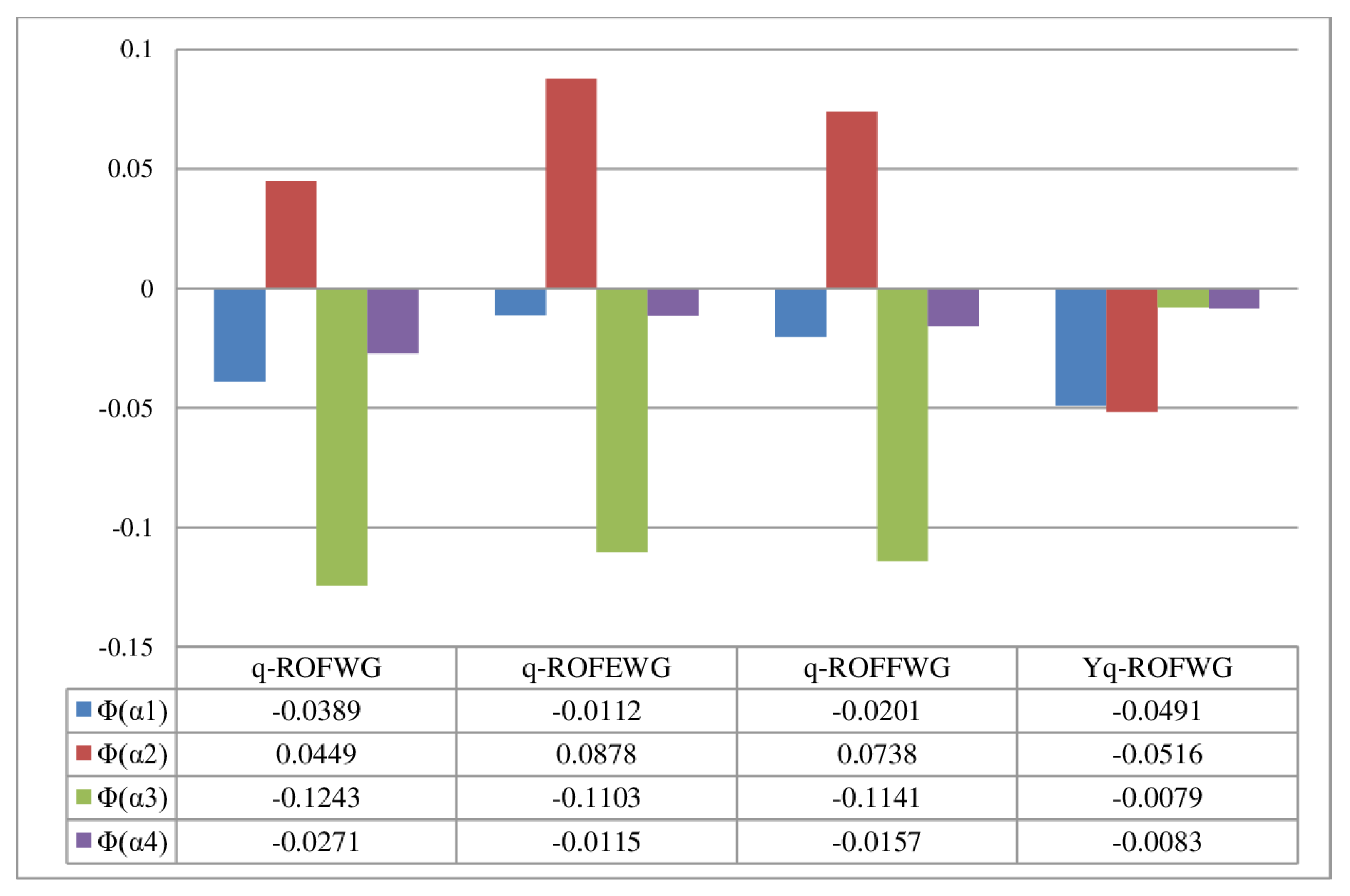
The score values $\mathsf{\Phi }\left({\alpha }_c\right)(c=1,2,3,4,5)$ using Definition 2 are given by: $\mathsf{\Phi }\left({\alpha }_1\right)$ = −0.0389, $\mathsf{\Phi }\left({\alpha }_2\right)$ = 0.0449, $\mathsf{\Phi }\left({\alpha }_3\right)$ = −0.1243, and $\mathsf{\Phi }\left({\alpha }_4\right)$ = −0.0271. Therefore, using the score values, we rank the four countries as ${\mathrm{Y}}_2>{\mathrm{Y}}_4>{\mathrm{Y}}_1>{\mathrm{Y}}_3.$

Step 6:

Therefore, the country ${\mathrm{Y}}_2$ possesses the highest rank among those four countries. So, the country ${\mathrm{Y}}_2$ is the most preferable country in which the MNC should build its software operating unit.

7. Comparison Analysis

In order to establish the validity and efficacy of the proposed model, we compared the outcomes obtained from our proposed method with those of several existing methods.

7.1. Comparison with Aggregation Operator-Based Methods

The calculation procedure for the IFWA [38] and EIFWA [38] is not very complicated, but its application field is confined. It can only handle decision-making problems with information expressed as an intuitionistic fuzzy number (IFN). Since our proposed MADM problem includes an evaluation value beyond the IFN, IFWA and EIFWA operators are insufficient to handle it. Now PFWA [42] and PFEWA [42] operators can only be used when the evaluation information is elicited as a PyFN. However, in PyFN, the square sum of MD and NMD is restricted to 1. As a result, the PFWA and PFEWG operators cannot be used to solve the given MADM problem. Now q-ROFWA, q-ROFEWA, q-ROFFWA, and Yq-ROFWA operators are most suitable to deal with the proposed model as the parameter q makes the aggregation process more adaptable. The range of information can be extended by increasing the parameter $q.$ As a result, we can say that our proposed model outperforms the models based on IFWA, EIFWA, PFWA, and PFEWG operators.

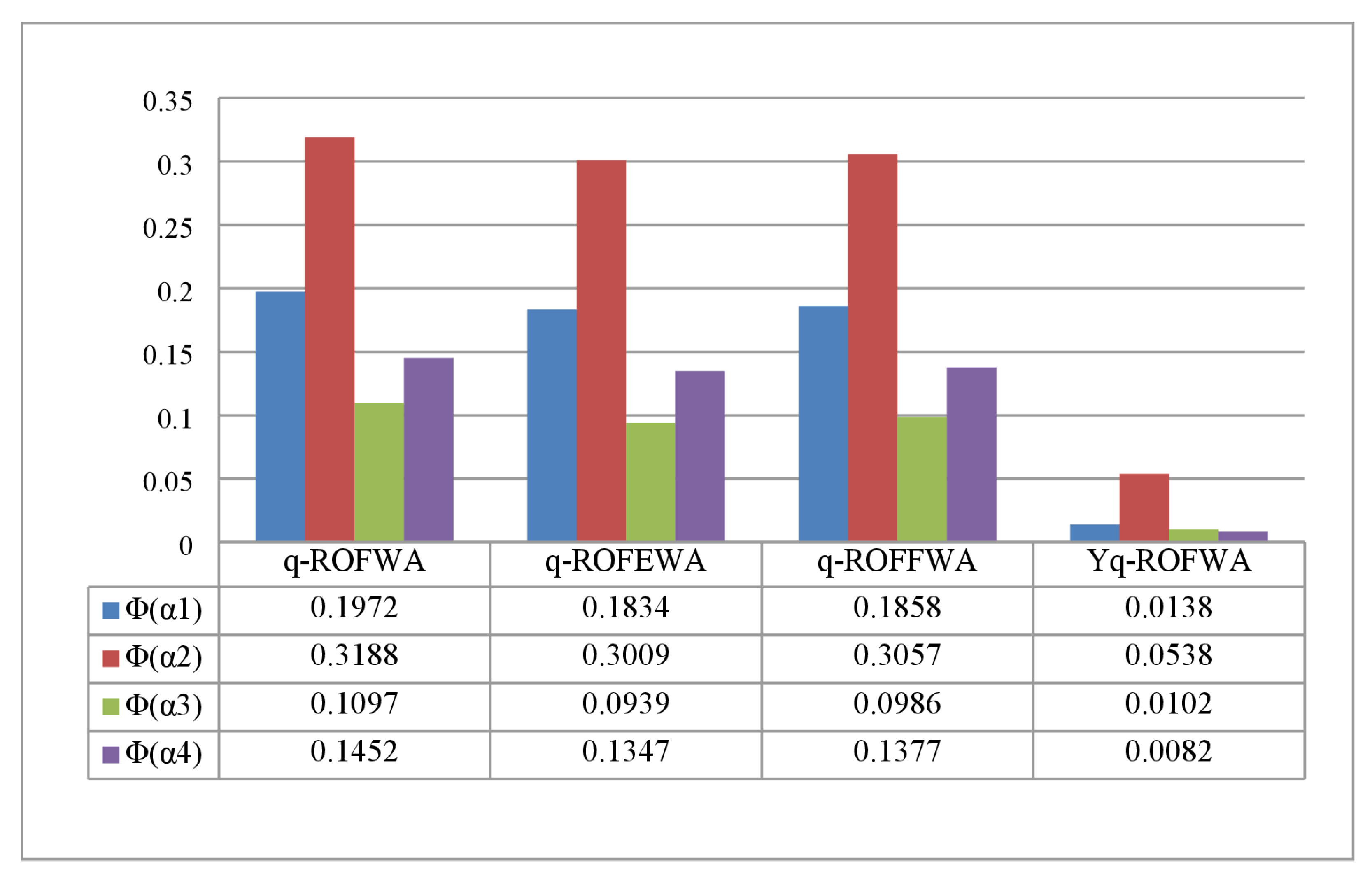
The appraisal score of every alternative is now computed using the q-ROFWA, q-ROFEWA, q-ROFFWA, and Yq-ROFWA operators. The alternatives are then ranked in descending order of score value. The ranking outcomes are shown in Figure 2 and

Table 8. Alternative rankings using some weighted averaging operators ($q=4$).

AOs	Score Values	Ranking Order	Best Option
IFWA [38]	cannot be determined	No	No
EIFWA [38]	cannot be determined	No	No
PFWA [42]	cannot be determined	No	No
PFEWA [43]	cannot be determined	No	No
q-ROFWA [34]	$\mathsf{\Phi }\left({\alpha }_1\right)$ = 0.1972, $\mathsf{\Phi }\left({\alpha }_2\right)$ = 0.3188, $\mathsf{\Phi }\left({\alpha }_3\right)$ = 0.1097,	${\mathrm{Y}}_2>{\mathrm{Y}}_1>{\mathrm{Y}}_4>{\mathrm{Y}}_3$	${\mathrm{Y}}_2$
	$\mathsf{\Phi }\left({\alpha }_4\right)$ = 0.1452
q-ROFEWA	$\mathsf{\Phi }\left({\alpha }_1\right)$ = 0.1834, $\mathsf{\Phi }\left({\alpha }_2\right)$ = 0.3009, $\mathsf{\Phi }\left({\alpha }_3\right)$ = 0.0939,	${\mathrm{Y}}_2>{\mathrm{Y}}_1>{\mathrm{Y}}_4>{\mathrm{Y}}_3$	${\mathrm{Y}}_2$
	$\mathsf{\Phi }\left({\alpha }_4\right)$ = 0.1347
q-ROFFWA	$\mathsf{\Phi }\left({\alpha }_1\right)$ = 0.1858, $\mathsf{\Phi }\left({\alpha }_2\right)$ = 0.3057, $\mathsf{\Phi }\left({\alpha }_3\right)$ = 0.0986,	${\mathrm{Y}}_2>{\mathrm{Y}}_1>{\mathrm{Y}}_4>{\mathrm{Y}}_3$	${\mathrm{Y}}_2$
$[\beta =3]$	$\mathsf{\Phi }\left({\alpha }_4\right)$ = 0.1377
Yq-ROFWA	$\mathsf{\Phi }\left({\alpha }_1\right)$ = 0.0138, $\mathsf{\Phi }\left({\alpha }_2\right)$ = 0.0538, $\mathsf{\Phi }\left({\alpha }_3\right)$ = 0.0102,	${\mathrm{Y}}_2>{\mathrm{Y}}_1>{\mathrm{Y}}_3>{\mathrm{Y}}_4$	${\mathrm{Y}}_2$
$[\beta =5]$	$\mathsf{\Phi }\left({\alpha }_4\right)$ = 0.0082

. From Figure 2 and Table 8, we observe that for the q-ROFWA, q-ROFEWA, and q-ROFFWA AOs ranking order is always ${\mathrm{Y}}_2>{\mathrm{Y}}_1>{\mathrm{Y}}_4>{\mathrm{Y}}_3$ and the optimal alternative is always ${\mathrm{Y}}_2$ although, the appraisal score for each alternative is different. Again, using Yq-ROFWA operator we obtain the ranking order as ${\mathrm{Y}}_2>{\mathrm{Y}}_1>{\mathrm{Y}}_3>{\mathrm{Y}}_4$ and the optimal alternative is ${\mathrm{Y}}_2.$

Now, we shall compare our result using q-ROFAWG using different additive generators $f.$ The ranking results using different geometric aggregation operators are displayed in Figure 3 and

Table 9. Alternative rankings using some weighted geometric operators ($q=4$).

AOs	Score Values	Ranking Order	Best Option
IFWG [39]	cannot be determined	No	No
EIFWG [41]	cannot be determined	No	No
PFWG [42]	cannot be determined	No	No
PFEWG [44]	cannot be determined	No	No
q-ROFWG [34]	$\mathsf{\Phi }\left({\alpha }_1\right)$ = −0.0389, $\mathsf{\Phi }\left({\alpha }_2\right)$ = 0.0449, $\mathsf{\Phi }\left({\alpha }_3\right)$ = −0.1243,	${\mathrm{Y}}_2>{\mathrm{Y}}_4>{\mathrm{Y}}_1>{\mathrm{Y}}_3$	${\mathrm{Y}}_2$
	$\mathsf{\Phi }\left({\alpha }_4\right)$ = −0.0271
q-ROFEWG	$\mathsf{\Phi }\left({\alpha }_1\right)$ = −0.0112, $\mathsf{\Phi }\left({\alpha }_2\right)$ = 0.0878, $\mathsf{\Phi }\left({\alpha }_3\right)$ = −0.1103,	${\mathrm{Y}}_2>{\mathrm{Y}}_1>{\mathrm{Y}}_4>{\mathrm{Y}}_3$	${\mathrm{Y}}_2$
	$\mathsf{\Phi }\left({\alpha }_4\right)$ = −0.0115
q-ROFFWG	$\mathsf{\Phi }\left({\alpha }_1\right)$ = −0.0201, $\mathsf{\Phi }\left({\alpha }_2\right)$ = 0.0738, $\mathsf{\Phi }\left({\alpha }_3\right)$ = −0.1141,	${\mathrm{Y}}_2>{\mathrm{Y}}_4>{\mathrm{Y}}_1>{\mathrm{Y}}_3$	${\mathrm{Y}}_2$
$[\beta =3]$	$\mathsf{\Phi }\left({\alpha }_4\right)$ = −0.0157
Yq-ROFWG	$\mathsf{\Phi }\left({\alpha }_1\right)$ = −0.0491, $\mathsf{\Phi }\left({\alpha }_2\right)$ = −0.0516, $\mathsf{\Phi }\left({\alpha }_3\right)$ = −0.0079,	${\mathrm{Y}}_4>{\mathrm{Y}}_3>{\mathrm{Y}}_1>{\mathrm{Y}}_2$	${\mathrm{Y}}_4$
$[\beta =5]$	$\mathsf{\Phi }\left({\alpha }_4\right)$ = −0.0083

.

From Table 9 and Figure 3, we see that the problem is not solvable by implementing IFWG, EIFWG, PFWG, and PFEWG AOs as they can only cope with IF information and Pythagorean fuzzy information. Again, utilizing q-ROFWG, q-ROFEWG, q-ROFFWG operators, we see that while the score values for the alternatives vary, their ranking order almost remains the same, and ${\mathrm{Y}}_2$ is the best option. Again, using Yq-ROFWG operator, we obtain the ranking order as ${\mathrm{Y}}_4>{\mathrm{Y}}_3>{\mathrm{Y}}_1>{\mathrm{Y}}_2$ and the optimal alternative is ${\mathrm{Y}}_4.$ The proposed procedure is more productive than conventional procedures for its flexibility to elicit fuzzy data in a wider range. Moreover, the existing approaches under the q-ROF environment are a particular case of our proposed approach. Therefore, our suggested MADM method is more generalized and compatible with q-ROFNs.

7.2. Comparison with q-ROF TOPSIS Method

In the literature, Alkan and Kahraman [45] extended the TOPSIS method based on a distance measure under the q-ROF environment. We call this approach Alkan and Kahraman’s method. This method is an effective model for solving MADM problems. Here, we apply the remaining steps of Alkan and Kahraman’s method to the normalized matrix N mentioned in Section 6.

At first, we determine the q-ROF weighted aggregated matrix by using the entropy weights. Let P be the weighted aggregated matrix. Then

$$P=\left(\begin{array}{ccccc}(0.557,0.875)& (0.409,0.709)& (0.476,0.741)& (0.576,0.924)& (0.444,0.935)\\ (0.656,0.875)& (0.566,0.719)& (0.403,0.839)& (0.462,0.977)& (0.474,0.845)\\ (0.333,0.875)& (0.409,0.929)& (0.557,0.958)& (0.550,0.777)& (0.132,0.935)\\ (0.232,0.960)& (0.409,0.901)& (0.491,0.875)& (0.568,0.771)& (0.490,0.922)\end{array}\right)$$

At first, we determine the q-ROF positive ideal solution (q-ROFPIS) and the IVSF negative ideal solution (q-ROFNIS). Let $X^{*}$ be the q-ROFPIS and $X^{-}$ be the q-ROFNIS. So, $X^{*}=\{(0.656,0.875),(0.566,0.719),(0.476,0.741),(0.568,0.771),(0.474,0.845)\}$ and

$X^{-}=\{(0.232,0.960),(0.409,0.979),(0.557,0.958),(0.462,0.977),(0.132,0.935)\}.$ Next, we compute the normalized Euclidean distance between the aggregated performance of alternative from the q-ROFPIS and q-ROFNIS which are denoted as $D_i^{+}({\mathrm{Y}}_i,X^{*})$ and $D_i^{-}({\mathrm{Y}}_i,X^{-})$, respectively. The values of $D_i^{+}({\mathrm{Y}}_i,X^{*})$ and $D_i^{-}({\mathrm{Y}}_i,X^{*}-)$ are exhibited in

Table 10. Outcomes of Alkan and Kahraman’s method.

Alternatives	${\mathit{D}}_{\mathit{i}}^{+}({\mathit{{\rm Y}}}_{\mathit{i}},{\mathit{X}}^{*})$	${\mathit{D}}_{\mathit{i}}^{-}({\mathit{{\rm Y}}}_{\mathit{i}},{\mathit{X}}^{*})$	${\mathit{CC}}_{\mathit{i}}\left({\mathit{{\rm Y}}}_{\mathit{i}}\right)$	Ranking
${\mathrm{Y}}_1$	0.434	0.333	0.434	3
${\mathrm{Y}}_2$	0.239	0.502	0.677	1
${\mathrm{Y}}_3$	0.466	0.311	0.400	4
${\mathrm{Y}}_4$	0.384	0.363	0.485	2

.

Finally, we calculate the relative closeness coefficient $C{C}_i\left({\mathrm{Y}}_i\right)$ for each alternative ${\mathrm{Y}}_i$ where $C{C}_i\left({\mathrm{Y}}_i\right)=\frac{D_i^{-}({\mathrm{Y}}_i,X^{-})}{D_i^{-}({\mathrm{Y}}_i,X^{-})+D_i^{+}({\mathrm{Y}}_i,X^{*})}.$ The values of $C{R}_i\left({\mathrm{Y}}_i\right)$ are displayed in Table 10. We exhibit the values of $C{C}_i\left({\mathrm{Y}}_i\right)$ in Table 10.

According to Table 10, ${\mathrm{Y}}_2\succ {\mathrm{Y}}_4\succ {\mathrm{Y}}_1\succ {\mathrm{Y}}_3$ is the ranking order of the four available alternatives. Therefore, ${\mathrm{Y}}_2$ is the best alternative obtained from Alkan and Kahraman’s method.

Therefore, the ranking of the alternatives using the proposed method and q-ROF TOPSIS method is almost the same. In both of the methods, the optimal alternative is always ${\mathrm{Y}}_2.$ The only difference is the ranking between ${\mathrm{Y}}_1$ and ${\mathrm{Y}}_4.$ In the q-ROF TOPSIS method ${\mathrm{Y}}_4\succ {\mathrm{Y}}_1,$ where in the proposed method ${\mathrm{Y}}_1\succ {\mathrm{Y}}_4.$ Therefore, the proposed method is highly reliable.

7.3. Comparison with q-ROF MULTIMOORA Method

Here, we compare the results of the developed method with the existing full multiplicative form (FMF) approach, the reference point (RP) approach, and the ratio system (RS) approach for the MULTIMOORA method [46] under the q-ROF environment. For this, the same numerical example is solved with the existing q-ROF environment MULTIMOORA method [46].

7.3.1. Comparison with RS Approach for q-ROF MULTIMOORA Method

Here, we apply the remaining steps of the RP approach for the MULTIMOORA method to the normalized matrix N mentioned in Section 6.

Then, we calculate the relative significance $\left(Y_i^{+}\right)$ for each alternative ${\mathrm{Y}}_i$ using q-ROFEWA operator [36]. The values of $Y_i^{+}$ are exhibited in

Table 11. Outcomes of RS approach for q-ROF-MULTIMOORA method.

Alternatives	${\mathit{Y}}_{\mathit{i}}^{+}$	$\mathbf{\Phi }\left({\mathit{Y}}_{\mathit{i}}^{+}\right)$	Ranking
${\mathrm{Y}}_1$	$(0.7289,0.5607)$	0.1834	2
${\mathrm{Y}}_2$	$(0.7635,0.4444)$	0.3009	1
${\mathrm{Y}}_3$	$(0.6698,0.5724)$	0.0939	4
${\mathrm{Y}}_4$	$(0.6864,0.5435)$	0.1347	3

.

Next, we defuzzify the $Y_i^{+}$ based on the score function given in Equation (1). Finally, we rank the alternatives based on $\mathsf{\Phi }\left(Y_i^{+}\right)$ values in descending order.

According to Table 11, we obtain the ranking outcome as ${\mathrm{Y}}_2\succ {\mathrm{Y}}_1\succ {\mathrm{Y}}_4\succ {\mathrm{Y}}_3$ Therefore, ${\mathrm{Y}}_2$ is the best alternative obtained from the RS approach for the q-ROF-MULTIMOORA method.

7.3.2. Comparison with FMF Approach for q-ROF MULTIMOORA Method

Here, we apply the remaining steps of the FMF approach for the MULTIMOORA method to the normalized matrix N mentioned in Section 6.

We calculate the total utility of the alternatives $\left(Z_i^{+}\right)$ for each alternative ${\mathrm{Y}}_i$ using the q-ROFEWGA operator [36]. The values of $Z_i^{+}$ are exhibited in

Table 12. Outcomes of FMF approach for the q-ROF-MULTIMOORA method.

Alternatives	${\mathit{Y}}_{\mathit{i}}^{+}$	$\mathbf{\Phi }\left({\mathit{Y}}_{\mathit{i}}^{+}\right)$	Ranking
${\mathrm{Y}}_1$	$(0.7114,0.7191)$	−0.0112	2
${\mathrm{Y}}_2$	$(0.7289,0.6641)$	0.0878	1
${\mathrm{Y}}_3$	$(0.5344,0.6619)$	−0.1103	4
${\mathrm{Y}}_4$	$(0.6226,0.6342)$	−0.0115	3

.

Next, we defuzzify the $Z_i^{+}$ based on the score function given in Equation (1). The score values of $Z_i^{+}$ are exhibited in Table 12. Finally, we rank the alternatives based on $\mathsf{\Phi }\left(Z_i^{+}\right)$ values in descending order.

According to Table 12, we obtain the ranking outcome as ${\mathrm{Y}}_2\succ {\mathrm{Y}}_1\succ {\mathrm{Y}}_4\succ {\mathrm{Y}}_3.$ Therefore, ${\mathrm{Y}}_2$ is the best alternative obtained from the FMF approach for the IVSF-MULTIMOORA method.

From Table 11 and Table 12, we can observe that the ranking of the four alternatives is ${\mathrm{Y}}_2\succ {\mathrm{Y}}_1\succ {\mathrm{Y}}_4\succ {\mathrm{Y}}_3,$ which is identical with the ranking obtained from the proposed methods. Therefore, our proposed model is highly reliable.

7.4. Validity Test

The same decision-making problem can produce different results for different MADM approaches. To illustrate the efficacy of our MADM approach, we check whether it satisfies the requirements set forth by Wang and Triantaphyllou [47] as:

Criterion 1:

If any non-optimal alternatives are replaced with worse alternatives while maintaining the level of significance of each attribute, the MADM approach remains efficient and the optimal alternative remains the same.

Criterion 2:

The transitivity law must be followed by an efficient MADM method.

Criterion 3:

If a MADM problem is divided into sub-problems, the given MADM problem can be used to rank the alternatives to those sub-problems. The joint ranking of the alternative remains unchanged from the previous ranking order.

Now, we testify in the following if our proposed method satisfies these criteria or not.

Test with Criterion 1

Here, a worse alternative ${\mathrm{Y}}_3$ is chosen arbitrarily and replaced by a new worse alternative ${\mathrm{Y}}_3^{\prime },$ where the q-ROF data for which the alternative ${\mathrm{Y}}_3^{\prime }$ satisfies the attributes ${\Im }_1,{\Im }_2,{\Im }_3,{\Im }_4,{\Im }_5$ are $(0.30,0.79),(0.55,0.49),(0.78,0.60),(0.70,0.40)$ and $(0.29,0.75)$, respectively. Depending on the modified information, the score values using the q-ROFEWA operator are obtained as $\mathsf{\Phi }\left({\alpha }_1\right)=0.2412$, $\mathsf{\Phi }\left({\alpha }_2\right)=0.2726$, $\mathsf{\Phi }\left({\alpha }_3^{\prime }\right)=0.0086$, and $\mathsf{\Phi }\left({\alpha }_4\right)=0.1302.$ The optimal ranking order is ${\mathrm{Y}}_2\succ {\mathrm{Y}}_1\succ {\mathrm{Y}}_4\succ {\mathrm{Y}}_3^{\prime }.$ This gives that still, ${\mathrm{Y}}_2$ is the optimal alternative. Again the score values using the q-ROFEWG operator are obtained as $\mathsf{\Phi }\left({\alpha }_1\right)=0.0868$, $\mathsf{\Phi }\left({\alpha }_2\right)=0.1049$, $\mathsf{\Phi }\left({\alpha }_3^{\prime }\right)=-0.1464$, and $\mathsf{\Phi }\left({\alpha }_4\right)=-0.0086.$ Which tells that still ${\mathrm{Y}}_2$ is the most suitable alternative. Hence, the proposed model meets this criterion. Similarly, if we implement other proposed operators, the proposed model meets this criterion.

7.5. Test with Other Criteria

If the MADM problem is divided into smaller sub-problems which consist of $\{{\mathrm{Y}}_1,{\mathrm{Y}}_2,{\mathrm{Y}}_3\}$, $\{{\mathrm{Y}}_2,{\mathrm{Y}}_3,{\mathrm{Y}}_4\}$, $\{{\mathrm{Y}}_3,{\mathrm{Y}}_4,{\mathrm{Y}}_1\}$ and $\{{\mathrm{Y}}_4,{\mathrm{Y}}_1,{\mathrm{Y}}_2\}$ alternatives. By solving each sub-problem with our suggested procedure, we acquire the alternatives’ ranking as ${\mathrm{Y}}_2\succ {\mathrm{Y}}_1\succ {\mathrm{Y}}_3,$ ${\mathrm{Y}}_2\succ {\mathrm{Y}}_3\succ {\mathrm{Y}}_4,$ ${\mathrm{Y}}_3\succ {\mathrm{Y}}_4\succ {\mathrm{Y}}_1,$ and ${\mathrm{Y}}_4\succ {\mathrm{Y}}_1\succ {\mathrm{Y}}_2$, respectively. In this manner, by combining them, we obtain ${\mathrm{Y}}_2\succ {\mathrm{Y}}_1\succ {\mathrm{Y}}_4\succ {\mathrm{Y}}_3$ which is similar to the original one. As a result, our method also meets the second and third requirements.

8. Conclusions

The q-ROFSs are more flexible for expressing ambiguous information because of the presence of the parameter $q.$ The Archimedean TCNs and TNs are generalizations of several TCNs and TNs. In this article, we have implemented the concepts of ATCN and ATN to develop AOs using q-ROF information. We have defined some novel operational rules for q-ROFNs utilizing ATCN and ATN. Thereafter, utilizing these operational laws, we propose q-ROFAWA, q-ROFAOWA, q-ROFAHA, q-ROFAWG, q-ROFAOWG, and q-ROFAHG operators. Afterward, the properties of these operators are thoroughly investigated. Next, we have shown that the AOs based on several existing TCNs and TNs (e.g., Frank, Hamacher, etc.) are particular cases of our proposed q-ROF AOs based on ATCN and ATN. Furthermore, we have presented a novel method to solve the MADM problem using the q-ROFAWA and q-ROFAWG operators. Finally, a numerical example of site selection of software operating units was used to show the feasibility, viability, and supremacy of the suggested approaches over other available methods.

There are some limitations to the current study. The primary limitation of this study is that the proposed model can only address the MADM issue. It can, however, be expanded to address MAGDM issues. Another shortcoming of this study is the computational complexity of the proposed model. However, this issue can be fixed by developing a computer program following the proposed approach, which will save decision-makers time and energy. Furthermore, the proposed MADM model is limited to the site selection problem. However, it is able to address other decision-making issues, e.g., sustainable development programs [48], plastic waste management process [49], job selection problems [5], bio-medical waste management [50], emergency assistance area selection [51], etc. Furthermore, the current study develops the Archimedean aggregation operators within the q-ROF context. However, the Archimedean aggregation operators can also be used in other fuzzy environments, e.g., the quasirung fuzzy environment [52,53], spherical fuzzy environment [54], etc.