A New Lomax Extension: Properties, Risk Analysis, Censored and Complete Goodness-of-Fit Validation Testing under Left-Skewed Insurance, Reliability and Medical Data

Abstract

The idea of symmetry, which is used to describe the shape of a probability distribution, is a key concept in the theory of probability. The use of symmetric and asymmetric distributions is common in statistical inference, decision-making, and probability calculations. This article introduces a novel asymmetric model for assessing risks under a skewed claims dataset. The new distribution is also employed for both censored and uncensored validation testing. Four estimation methods, maximum likelihood, ordinary least squares, L-Moment, and Anderson Darling, were used for the risk assessment and analysis. To explain the exposure to risk within actuarial claims data, we introduced five crucial indicators, namely value-at-risk, tail-value-at-risk, tail variance, tail mean-variance, and mean excess losses. A numerical and graphical analysis is presented to assess the actuarial risk. Furthermore, the article discusses a newly developed Rao Robson Nikulin statistic for censored and uncensored validation testing. The validation testing also involved the insurance claims dataset.

1. Introduction

Skewed distributions can have important implications for statistical analysis. For example, if the data are positively skewed, the mean may not be a good measure of central tendency, as it will be influenced by the few extreme values on the right-hand side of the distribution. In this case, the median may be a better measure of central tendency. Similarly, if the data are negatively skewed, the mean may be lower than expected, and again, the median may be a better measure of central tendency. In a negatively skewed distribution, the mean is less than the median, and the tail of the distribution is longer on the left-hand side. This means that there are more data points on the right-hand side of the distribution than on the left-hand side. An example of a negatively skewed distribution is the distribution of reaction times, where most people react quickly, but a few people take a long time to react (see Aboraya et al. [1], Acerbi and Tasche [2]).

Following Adcock et al. [3], Eling [4] and Ali et al. [5,6], the concept of symmetry refers to the shape of a probability distribution. When the left and right sides of a probability distribution mirror the other side exactly, the distribution is said to be symmetric. Or, to put it another way, the left and right sides of the distribution would be identical if a vertical line were drawn down the center of it. The most well-known illustration of a symmetric distribution is probably the normal distribution. In the study of statistics, the normal distribution is commonly used to describe a wide range of real-world events. The mean and the median are both located in the center of the bell-shaped curve that symbolizes the normal distribution. Because of the distribution’s symmetry, the mean, median, and mode are the same in a normal distribution. As a result, symmetry plays a crucial role in the definition of a probability distribution’s shape in the field of probability theory. Anything from a circle to a bell curve might be this shape. Symmetric distributions are commonly used in the areas of statistical inference, decision-making, and probability computation. However, not all distributions are symmetric, and probability theory also heavily utilizes asymmetric distributions, also referred to as skewed distributions.

This study investigates a new model called the generalized exponential Lomax (GELX) for the negatively skewed insurance data. The new model is a new generalization of the well-known Lomax (LX) model. A random variable (RV) $\mathcal{Z}$ has the LX distribution if it has cumulative distribution function (CDF) (for $𝓏>0$) given by

$$H_{\beta }\left(\mathcal{z}\right){|}_{\left(\beta >0\right)}=1-{\phi }_{\beta }\left(\mathcal{z}\right),$$

(1)

where ${\phi }_{\beta }\left(\mathcal{z}\right)={\left(1+\frac{1}{2}\mathcal{z}\right)}^{-\beta }$ and $\beta$ refers to the shape parameter. The scale parameter is considered as 2 for reducing the number of the parameters. Then, the corresponding probability density function (PDF) of (1) is

$$h_{\beta }\left(\mathcal{z}\right)=\frac{1}{2}\beta {\left(1+\frac{1}{2}\mathcal{z}\right)}^{-\left(\beta +1\right)}.$$

(2)

Based on Alizadeh et al. [7], the CDF and PDF of GELX model is given, respectively, by

$$F_{\underset{\_}{\mathcal{V}}}\left(\mathcal{z}\right)={\left[1-exp\left\{-{\left[{\psi }_{{\delta }_2,\beta }\left(\mathcal{z}\right)-1\right]}^{-1}\right\}\right]}^{{\delta }_1}{|}_{\underset{\_}{\mathcal{V}}={\delta }_1,{\delta }_2,\beta },$$

(3)

where $\underset{\_}{\mathcal{V}}=\left({\delta }_1,{\delta }_2,\beta \right)$, ${\psi }_{{\delta }_2,\beta }\left(\mathcal{z}\right)={\left[1-{\phi }_{\beta }\left(\mathcal{z}\right)\right]}^{-{\delta }_2}$ and

$$f_{\underset{\_}{\mathcal{V}}}\left(\mathcal{z}\right)={\delta }_1{\delta }_2\frac{\beta }{2}\frac{{\left[1-{\phi }_{\beta }\left(\mathcal{z}\right)\right]}^{{\delta }_2-1}{\left(1+\frac{1}{2}\mathcal{z}\right)}^{-\left(\beta +1\right)}}{{\left\{1-{\left[1-{\phi }_{\beta }\left(\mathcal{z}\right)\right]}^{{\delta }_2}\right\}}^{2}exp\left\{{\left[{\psi }_{{\delta }_2,\beta }\left(\mathcal{z}\right)-1\right]}^{-1}\right\}}\underset{A_{{\delta }_1,{\delta }_2,\beta }\left(\mathcal{z}\right)}{\underbrace{{\left[1-exp\left\{-{\left[{\psi }_{{\delta }_2,\beta }\left(\mathcal{z}\right)-1\right]}^{-1}\right\}\right]}^{{\delta }_1-1}}},$$

(4)

where ${\delta }_1,{\delta }_2>0$ are two additional shape parameters. Henceforth, $\mathcal{Z}\sim$ GELX($\underset{\_}{\mathcal{V}}$) denotes an RV having density function (4). The reliability function (rf) and hazard rate function (HRF) of $\mathcal{Z}$ are, respectively, given by $h_{\underset{\_}{\mathcal{V}}}\left(\mathcal{z}\right)=f_{\underset{\_}{\mathcal{V}}}\left(\mathcal{z}\right)/R_{\underset{\_}{\mathcal{V}}}\left(\mathcal{z}\right)$, where $R_{\underset{\_}{\mathcal{V}}}\left(\mathcal{z}\right)=1-F_{\underset{\_}{\mathcal{V}}}\left(\mathcal{z}\right).$

In this paper, we employ the new model in (4) in two significant directions which are the risk analysis and distributional validity. The use of probability-based distributions to describe risk exposure is an important new statistical direction. Typically, a single number or a small set of numbers, known as key risk indicators (KRIs), are used to represent the level of risk exposure. The KRIs serve as a valuable tool for actuaries and risk managers by providing information about the extent to which a company is exposed to specific risks. Various KRIs, such as value-at-risk (VaRK), tail-value-at-risk (TVaRK), conditional-value-at-risk (CVaRK), tail variance (TV), and tail mean-variance (TMV), can be analyzed. For the risk validation, the Rao–Robson Nikulin (RRNIK) test statistic (see Nikulin [8], Nikulin [9], Nikulin [10], and Rao and Robson [11]) is used for uncensored validation. On the other hand, a new modified version of the RRNIK test statistic is used for the censored validation. Finally, the actuarial datasets are examined for validation under the RRNIK test statistic. These risk indicators help investors and risk managers make informed decisions by quantifying and assessing the potential downside risk of investments. They contribute to a more comprehensive understanding of risk and support the development of robust risk management strategies.

The following reasons are the primary drivers driving the introduction of this new distribution:

I.

We created a new probability distribution with only three parameters for validation and risk analysis. For applied modeling, estimation, simulation trials, etc., the fewer the distribution parameters, the better.

II.

A new probability distribution is presented with simple mathematical features that make it simple to compute and use. The quantile function is the only mathematical or statistical property of the present distribution that cannot be obtained in precise formulas, as will be demonstrated later. The latest statistical programs such as “R” and “Mathcad”, however, greatly aid in overcoming this issue with numerical approaches and fixes. In these circumstances, it is essential to comprehend numerical methods (and the numerical solutions they provide) in order to get around some of the more difficult formulations that researchers may run against.

III.

We examined numerous traditional estimation techniques in light of the new distribution, either through simulative experiments or through real-world applications.

IV.

The majority of practical statistical work must include the new distributions into the modeling procedures. In this work, we did this by employing an old, well-known goodness-of-fit test and a new, modified goodness-of-fit test, and we gave evidence and justifications in support of the validity of the new modified test as well as the significance of the new distribution.

V.

We examined the new distribution from a number of perspectives in order to better understand it, including the mathematical side, the modeling side, the estimation and simulation processes in various ways, and the statistical hypothesis tests.

In fact, the specialized literature has a good number of extensions of the LX distribution, and these extensions were mostly used in mathematical and statistical modeling processes. The Lomax distribution is often used to model extreme events or rare occurrences that fall in the upper tail of a distribution. In actuarial sciences, extreme events are of particular interest since they often represent catastrophic or high-impact events such as insurance claims, natural disasters, or financial losses. The Lomax distribution provides a flexible framework for modeling the tail behavior of these events and estimating their probabilities. Actuaries play a crucial role in the insurance industry by assessing and managing risks. The Lomax distribution is often employed in insurance modeling, particularly in areas such as property and casualty insurance. It helps actuaries estimate the likelihood and severity of extreme events, which is essential for determining appropriate insurance premiums, policy limits, and reserves (see Aboraya et al. [1]).

Actuarial risk analysis involves modeling the frequency and severity of losses or claims. The Lomax distribution can be used to model the severity component, representing the distribution of individual claim sizes or losses. By fitting the Lomax distribution to historical data, actuaries can gain insights into the statistical properties of losses and make informed decisions regarding risk management and pricing. Actuarial risk analysis involves estimating extreme quantiles, such as value-at-risk or Conditional Tail Expectation, which are used to assess the potential losses or liabilities associated with extreme events. The Lomax distribution can be fitted to historical data or used in combination with other models to estimate these tail quantiles accurately. Its tail heaviness allows for the extreme values and tail behavior of the data to be captured better (see Wirch [12] and Tasche [13]). The LX distribution serves as a useful tool for actuarial science researchers. It provides a flexible framework for studying extreme value theory, analyzing heavy-tailed distributions, and developing new statistical models for actuarial risk. Researchers can explore various aspects of risk analysis, such as dependence modeling, copulas, multivariate extensions, and time series modeling, using the Lomax distribution as a building block. For more details, regression models, applications, and real datasets, see Butt and Khalil [14] for a novel skewed bimodal model for modeling the asymmetric heavy-tail bimodal datasets, Reyes et al. [15] for a new bimodal exponential extension with some applications in risk theory, and Gómez et al. 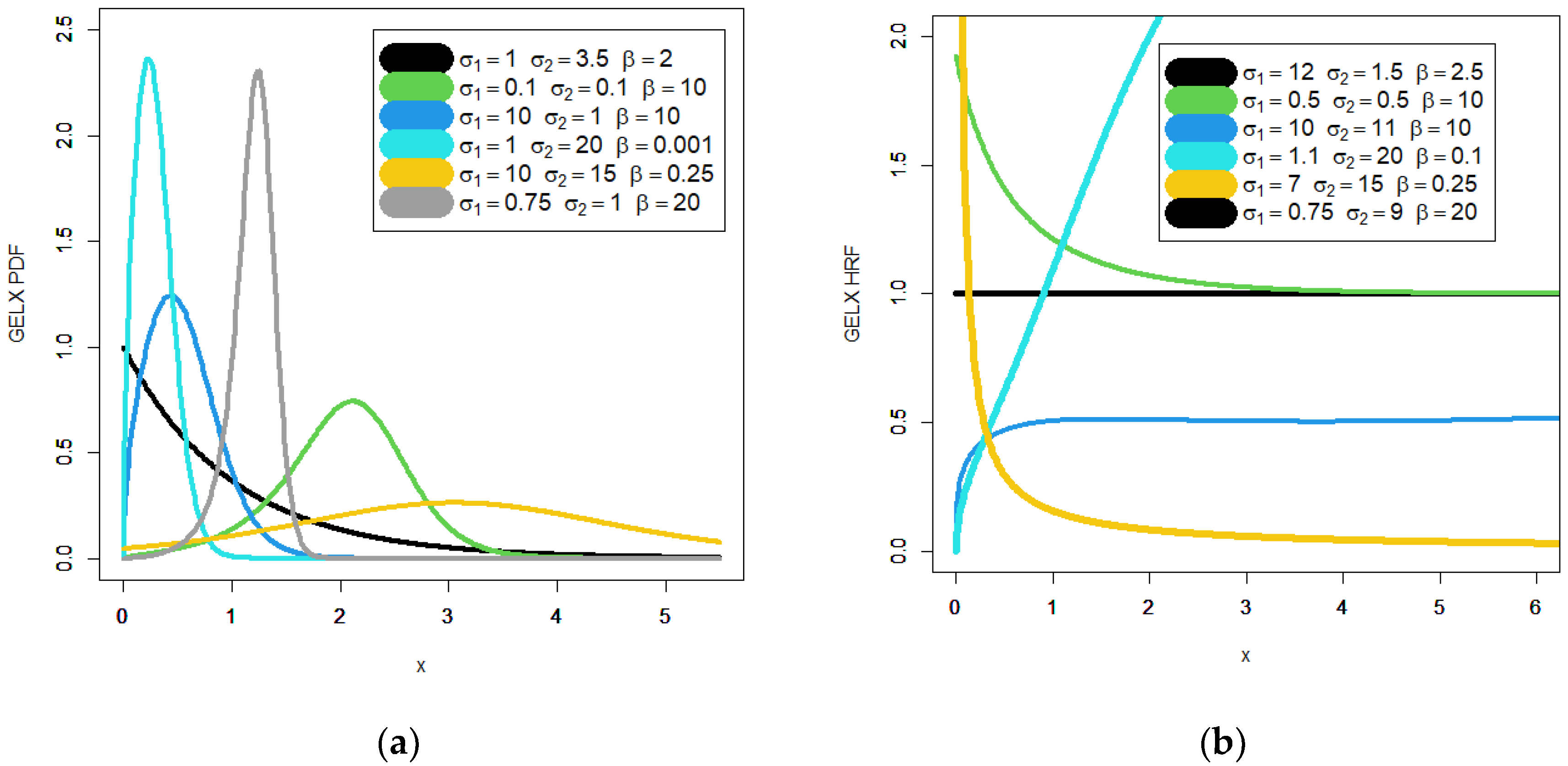[16] for asymmetric bimodal double-regression modeling. A few plots of the GELX PDF and HRF are shown in Figure 1. We conclude from Figure 1′s left panel that the PDF of the GELX distribution displays a variety of significant forms with varied kurtosis values. Based on Figure 1a, it is seen that the new PDF can be symmetric with one peak, asymmetric with one peak and right skewed with no peak. Based on Figure 1b, it is seen that the new HRF can be constant, decreasing, increasing, and increasing–constant.

Section 2 presents some mathematical properties of the new model. Section 3 presents the KRIs. The risk assessment using different estimation methods is given in Section 4. A case study is illustrated in Section 5. The construction of the RRNIK statistic for the GELX model is given in Section 6. Section 7 and Section 8 give the uncensored and censored distributional validations, respectively. Section 9 offers some concluding remarks.

2. Mathematical Properties

First, we give a simple formula for (4). Using the following series expansion which holds for $\left|\frac{{\mathit{\zeta }}_1}{{\mathit{\zeta }}_2}\right|<\mathbf{1}$ and $\hspace{1em}{\mathit{\zeta }}_3>\mathbf{0}$ real non-integer

$${\left(\mathbf{1}-\frac{{\mathit{\zeta }}_{\mathbf{1}}}{{\mathit{\zeta }}_{\mathbf{2}}}\right)}^{{\mathit{\zeta }}_{\mathbf{3}}-\mathbf{1}}=\stackrel{\mathbf{\infty }}{{\displaystyle \sum }_{{\mathit{\zeta }}_{\mathbf{4}}=\mathbf{0}}}{\left(-{\mathit{\zeta }}_{\mathbf{1}}\right)}^{{\mathit{\zeta }}_{\mathbf{4}}}\left(\begin{array}{c}{\mathit{\zeta }}_{\mathbf{3}}-\mathbf{1}\\ {\mathit{\zeta }}_{\mathbf{4}}\end{array}\right){\left(\frac{\mathbf{1}}{{\mathit{\zeta }}_{\mathbf{2}}}\right)}^{{\mathit{\zeta }}_{\mathbf{4}}},$$

to expand the quantity $A_{{\delta }_1,{\delta }_2,\beta }\left(\mathcal{z}\right),$ we obtain

$$A_{{\delta }_1,{\delta }_2,\beta }\left(\mathcal{z}\right)=\stackrel{\infty }{{\displaystyle \sum }_{i=0}}{\left(-1\right)}^i\left(\begin{array}{c}{\delta }_1-1\\ i\end{array}\right)exp\left(-i{\left\{{\psi }_{{\delta }_2,\beta }\left(\mathcal{z}\right)-1\right\}}^{-1}\right).$$

Then, the novel PDF in (4) can be derived as

$$f_{\underset{\_}{\mathcal{V}}}\left(\mathcal{z}\right)={\delta }_1{\delta }_2\frac{\beta }{2}\frac{{\left[1-{\phi }_{\beta }\left(\mathcal{z}\right)\right]}^{{\delta }_2-1}}{{\left\{1-{\left[1-{\phi }_{\beta }\left(\mathcal{z}\right)\right]}^{{\delta }_2}\right\}}^2}\stackrel{\infty }{{\displaystyle \sum }_{i=0}}{\left(-1\right)}^i\left(\begin{array}{c}{\delta }_1-1\\ i\end{array}\right){\left(1+\frac{1}{2}\mathcal{z}\right)}^{-\left(\beta +1\right)}\underset{B_{{\delta }_2,\beta }\left(\mathcal{z}\right)}{\underbrace{exp\left(-\left(1+i\right){\left\{{\psi }_{{\delta }_2,\beta }\left(\mathcal{z}\right)-1\right\}}^{-1}\right)}}.$$

Expanding the quantity $B_{{\delta }_2,\beta }\left(\mathcal{z}\right)$ using the power series$,$ we obtain

$$B_{{\delta }_2,\beta }\left(\mathcal{z}\right)=\stackrel{\infty }{{\displaystyle \sum }_{d_1=0}}{\left(-1\right)}^{d_1}\frac{{\left(1+i\right)}^{d_1}}{d_1!}\left(\frac{{\left[1-{\phi }_{\beta }\left(\mathcal{z}\right)\right]}^{{\delta }_2{d}_1}}{{\left\{1-{\left[1-{\phi }_{\beta }\left(\mathcal{z}\right)\right]}^{{\delta }_2}\right\}}^{d_1}}\right).$$

Then, the PDF in (4) can be formulated as

$$f_{\underset{\_}{\mathcal{V}}}\left(\mathcal{z}\right)={\delta }_1{\delta }_2\frac{\beta }{2}\stackrel{\infty }{{\displaystyle \sum }_{i,d_1=0}}\frac{{\left(-1\right)}^{i+d_1}{\left(1+i\right)}^{d_1}{\left[1-{\phi }_{\beta }\left(\mathcal{z}\right)\right]}^{{\delta }_2\left(d_1+1\right)-1}}{d_1!\underset{C_{d_1,{\delta }_2,\beta }\left(\mathcal{z}\right)}{\underbrace{{\left\{1-{\left[1-{\phi }_{\beta }\left(\mathcal{z}\right)\right]}^{{\delta }_2}\right\}}^{2+d_1}}}}\left(\begin{array}{c}{\delta }_1-1\\ i\end{array}\right){\left(1+\frac{1}{2}\mathcal{z}\right)}^{-\left(\beta +1\right)}.$$

We apply the series expansion again to the quantity $C_{d_1,{\delta }_2,\beta }\left(\mathcal{z}\right)$. Then, we can obtain

$$f_{\underset{\_}{\mathcal{V}}}\left(\mathcal{z}\right)=\stackrel{\infty }{{\displaystyle \sum }_{d_1,d_2=0}}{w}_{d_1,d_2} h_{{\delta }^{\ast },\beta }\left(\mathcal{z}\right){|}_{{\delta }^{\ast }={\delta }_2\left(d_1+d_2+1\right)},$$

(5)

where $h_{{\delta }^{\ast },\beta }\left(\mathcal{z}\right)=\frac{1}{2}\xi a^{\ast }{\left[1-{\phi }_{\beta }\left(\mathcal{z}\right)\right]}^{{\delta }^{\ast }-1}{\left(1+\frac{1}{2}\mathcal{z}\right)}^{-\left(\beta +1\right)}$ represents the PDF of the exp-LX model with power parameter ${\delta }^{\ast }$ and

$$w_{d_1,d_2}=\frac{{\delta }_1{\delta }_2}{d_1!{\delta }^{\ast }}{\left(-1\right)}^{d_1+d_2}\left(\begin{array}{c}-\left(d_1+2\right)\\ d_2\end{array}\right)\stackrel{\infty }{{\displaystyle \sum }_{i=0}}{\left(-1\right)}^i{\left(i+1\right)}^{d_1}\left(\begin{array}{c}{\delta }_1-1\\ i\end{array}\right).$$

The CDF of the GELX model can also be expressed as a mixture of exponentiated Lomax (ELX) CDFs. By integrating (4), we obtain the same mixture representation

$$F_{\underset{\_}{\mathcal{V}}}\left(\mathcal{z}\right)=\stackrel{\infty }{{\displaystyle \sum }_{d_1,d_2=0}}{w}_{d_1,d_2}{H}_{{\delta }^{\ast },\beta }\left(\mathcal{z}\right){|}_{{\delta }^{\ast }={\delta }_2\left(d_1+d_2+1\right)},$$

(6)

where $H_{{\delta }^{\ast },\beta }\left(\mathcal{z}\right)={\left[1-{\phi }_{\beta }\left(\mathcal{z}\right)\right]}^{{\delta }^{\ast }}$ is the CDF of the ELX model with power parameter ${\delta }^{\ast }$. The stochastic properties of probability distributions are important because they describe the behavior of random variables and stochastic processes. These properties are used to model and analyze a wide range of real-world phenomena, from stock prices to weather patterns to the behavior of subatomic particles.

Stochastic properties are used to model the uncertainty of and variability in financial assets and to analyze the risk associated with investments. The mean and variance of probability distributions are used to calculate the expected return and risk of a portfolio of assets.

3. The KRIs

The VaRK is a widely used risk indicator that estimates the maximum potential loss within a specified confidence level over a given time horizon. It provides a single number that represents the worst-case loss a portfolio or investment is expected to experience. VaRK helps investors assess and compare the riskiness of different assets or portfolios and set risk management limits. It is particularly useful in risk measurement, risk monitoring, and regulatory compliance; see Wirch [12], Tasche [13], and Acerbi and Tasche [2] for more details and applications. We can simply obtain the quantity VaR$\left(\mathcal{z}\right)$ for the GELX distribution from the following probability:

$$\stackrel{}{\mathrm{Pr}}\left\{\mathcal{Z}>2\left[{\left(1-{\left\{-\mathcal{q}\left({\delta }_1\right)/\left[1-\mathcal{q}\left({\delta }_1\right)\right]\right\}}^{\frac{1}{{\delta }_2}}\right)}^{-\frac{1}{\beta }}-1\right]\right\}=\{\begin{array}{l}1\%{|}_{\mathcal{q}=99\%}\hspace{1em}\\ 5\%{|}_{\mathcal{q}=95\%}\hspace{1em}\\ ⋮\hspace{1em}\end{array},$$

(7)

where $\mathcal{q}\left({\delta }_1\right)=log\left(1-{\mathcal{q}}^{\frac{1}{{\delta }_1}}\right).$.

The TVaRK, which is also known as conditional value-at-risk (CVaR), is an extension of VaR by considering the expected loss beyond the VaRK threshold. Unlike VaR, which only measures the loss at a specific confidence level, TVaRK estimates the average loss in the tail of the distribution (see Hogg and Klugman [17], Klugman et al. [18], Lane [19], McNeil et al. [20], Vernic [21], Artzner [22], and Charpentier [23]). This risk indicator provides additional information about extreme losses and tail risks. TVaRK is often used to evaluate downside risk and is popular in risk measurement, risk budgeting, and portfolio optimization. The $\mathrm{TVaRK}\left(\mathcal{Z}\right)$ can also be derived due to the main result below as

$$\mathrm{TVaRK}\left(\mathcal{Z}\right)=E\left(\mathcal{Z}|\mathcal{Z}>\pi \left(\mathcal{q}\right)\right)=\frac{1}{1-F_{\underset{\_}{\mathcal{V}}}\left(\pi \left(\mathcal{q}\right)\right)}{{\displaystyle \int }}_{\pi \left(\mathcal{q}\right)}^{\infty }\mathcal{z}{f}_{\underset{\_}{\mathcal{V}}}\left(\mathcal{z}\right)d\mathcal{z},$$

which can be simplified to

$$\mathrm{TVaRK}\left(\mathcal{Z}\right)=\frac{1}{1-\mathcal{q}}{{\displaystyle \int }}_{\pi \left(\mathcal{q}\right)}^{\infty }\mathcal{z}{f}_{\underset{\_}{\mathcal{V}}}\left(\mathcal{z}\right)d\mathcal{z}.$$

(8)

Then, using (5), we reach

$$\mathrm{TVaRK}\left(\mathcal{Z}\right)=\frac{1}{1-\mathcal{q}}\stackrel{\infty }{{\displaystyle \sum }_{d_1,d_2=0}}{\displaystyle \sum }_{d_3=0}^1{\Upsilon }_{d_1,d_2,d_3}^{\left(1,{\delta }^{\ast }\right)}\left[\begin{array}{c}B\left({\delta }^{\ast },1+\frac{d_3-1}{\beta }\right)\\ -B_{\pi \left(\mathcal{q}\right)}\left({\delta }^{\ast },1+\frac{d_3-1}{\beta }\right)\end{array}\right]{|}_{\left(\beta >1\right)},$$

(9)

where

$${\Upsilon }_{d_1,d_2,d_3}^{\left(1,{\delta }^{\ast }\right)}=2w_{d_1,d_2}{\delta }^{\ast }{\left(-1\right)}^{d_3}\left(\begin{array}{c}1\\ d_3\end{array}\right),$$

$$B\left(1+{\Upsilon }_1,1+{\Upsilon }_2\right)={{\displaystyle \int }}_0^1{\mathcal{z}}^{{\Upsilon }_1}{\left(1-\mathcal{z}\right)}^{{\Upsilon }_2}d\mathcal{z}, \mathrm{and} B_{\pi \left(\mathcal{q}\right)}\left(1+{\Upsilon }_1,1+{\Upsilon }_2\right)={{\displaystyle \int }}_0^{\pi \left(\mathcal{q}\right)}{\mathcal{z}}^{{\Upsilon }_1}{\left(1-\mathcal{z}\right)}^{{\Upsilon }_2}d\mathcal{z}.$$

Thus, the quantity TVaRK$\left(\mathcal{z}\right)$ is an average of all VaRK values above the confidence level $\mathcal{q}$, which provides more information about the tail of the GELX distribution. Further, it can also be expressed as

$$\mathrm{TVaRK}\left(\mathcal{Z}\right)=\mathrm{VaRK} \left(\mathcal{Z}\right)+e\left(\mathrm{VaRK} \left(\mathcal{Z}\right)\right),$$

(10)

where $e\left(\mathrm{VaRK} \left(\mathcal{Z}\right)\right)$ is the mean excess loss function evaluated at the $100\mathcal{q}\%$ th quantile. So, TVaRK$\left(\mathcal{Z}\right)$ is larger than its corresponding VaRK$\left(\mathcal{Z}\right)$ by the amount of average excess of all losses that exceed the MELS$\left(\mathcal{Z}\right)$ value of VaRK$\left(\mathcal{Z}\right)$ (see Acerbi and Tasche [2], Wirch [12], and Tasche [13] for more details and applications). Tail variance measures the variability in or dispersion of returns in the extreme tails of the distribution. It focuses on the higher moments of the distribution beyond the mean and standard deviation. The TV provides information about the thickness and shape of the tails, helping investors gauge the potential losses in extreme market conditions. It is particularly useful in assessing tail risk, designing risk management strategies, and constructing tail risk hedging instruments. Following Furman and Landsman [24], the TV risk indicator can be derived due to the following formula:

$$\mathrm{TVq}\left(\mathcal{Z}\right)=E\left({\mathcal{Z}}^2|\mathcal{Z}>\pi \left(\mathcal{q}\right)\right)-{\left[\mathrm{TVaRK}\left(\mathcal{Z}\right)\right]}^2;$$

(11)

then, using (6) we reach

$$E\left({\mathcal{Z}}^2|\mathcal{Z}>\pi \left(\mathcal{q}\right)\right)=\frac{1}{1-\mathcal{q}}\stackrel{\infty }{{\displaystyle \sum }_{d_1,d_2=0}}{\displaystyle \sum }_{d_3=0}^2{\Upsilon }_{d_1,d_2,d_3}^{\left(2,{\delta }^{\ast }\right)}\left[\begin{array}{c}B\left({\delta }^{\ast },1+\frac{d_3-2}{\beta }\right)\\ -B_{\pi \left(\mathcal{q}\right)}\left({\delta }^{\ast },1+\frac{d_3-2}{\beta }\right)\end{array}\right]{|}_{\left(\beta >2\right)},$$

(12)

and ${\Upsilon }_{d_1,d_2,d_3}^{\left(2,{\delta }^{\ast }\right)}=4w_{d_1,d_2}{\delta }^{\ast }{\left(-1\right)}^{d_3}\left(\begin{array}{c}2\\ d_3\end{array}\right).$ Inserting (9) and (12) in (11), the TVq$\left(\mathcal{Z};\underset{\_}{\mathcal{V}}\right)$ can be expressed as

$$\mathrm{TVq}\left(\mathcal{Z};\underset{\_}{\mathcal{V}}\right)=\frac{1}{1-\mathcal{q}}\left(\begin{array}{c}{\displaystyle {\displaystyle \sum }_{d_1,d_2=0}^{\infty }}{\displaystyle {\displaystyle \sum }_{d_3=0}^2}{\Upsilon }_{d_1,d_2,d_3}^{\left(2,{\delta }^{\ast }\right)}\left[\begin{array}{c}B\left({\delta }^{\ast },1+\frac{d_3-2}{\beta }\right)\\ -B_{\pi \left(\mathcal{q}\right)}\left({\delta }^{\ast },1+\frac{d_3-2}{\beta }\right)\end{array}\right]\\ -\frac{1}{1-\mathcal{q}}{\left\{{\displaystyle {\displaystyle \sum }_{d_1,d_2=0}^{\infty }}{\displaystyle {\displaystyle \sum }_{d_3=0}^1}{\Upsilon }_{d_1,d_2,d_3}^{\left(1,{\delta }^{\ast }\right)}\left[\begin{array}{c}B\left({\delta }^{\ast },1+\frac{d_3-1}{\beta }\right)\\ -B_{\pi \left(\mathcal{q}\right)}\left({\delta }^{\ast },1+\frac{d_3-1}{\beta }\right)\end{array}\right]\right\}}^2\end{array}\right).$$

(13)

The TMVK analysis combines elements of mean-variance analysis with a focus on the tail of the distribution. It considers the trade-off between expected return and risk, specifically targeting the downside risk associated with extreme losses. By incorporating tail risk measures, such as TVaRK or tail variance, into the traditional mean-variance framework, investors can construct portfolios that optimize risk-adjusted returns, giving more weight to the tail behavior of the returns distribution. Following Landsman [25], the TMVK risk can be expressed as

$$\mathrm{TMVK}\left(\mathcal{Z},\varsigma \right)=\mathrm{TVaRK}\left(\mathcal{Z}\right)+\varsigma \mathrm{TVq}\left(\mathcal{Z}\right){|}_{0<\varsigma <1}.$$

(14)

Then, for any LRV, TMVK$\left(\mathcal{Z},\varsigma \right)>$ TVq$\left(\mathcal{Z}\right)$ and, for $\varsigma =0$, $\mathrm{TMVK}\left(\mathcal{Z}\right)=$ TVaRK$\left(\mathcal{Z}\right).$ For more applications, see Punzo [26] and Punzo et al. [27,28].

4. Risk Assessment Using Different Estimation Methods

In this section, we consider the following estimation methods—maximum likelihood estimation (MAXLE), ordinary least squares (OLS), L-Moment (L-MO), and Anderson Darling estimation (ADE)—for calculating the KRIs. These quantities are estimated using $N=1000$ with different sample sizes $\left(n=50, 150, 300, 500\right)$ and three confidence levels (CLs) ($\mathcal{q}=\left(70\%,90\%,99\%\right)$). All results are calculated and checked using the Mathcad program and reported in

Table 1. Simulated KRIs for assessing the artificial data when n = 50.

Method				$\mathrm{VaRK}\left(\mathcal{Z};\widehat{\underset{\_}{\mathcal{V}}}\right)$	$\mathbf{TVaRK}\left(\mathcal{Z};\widehat{\underset{\_}{\mathcal{V}}}\right)$	$\mathbf{TVq}\left(\mathcal{Z};\widehat{\underset{\_}{\mathcal{V}}}\right)$	$\mathrm{TMVK}\left(\mathcal{Z};\widehat{\underset{\_}{\mathcal{V}}}\right)$	$\mathrm{MELS}\left(\mathcal{Z};\widehat{\underset{\_}{\mathcal{V}}}\right)$
MAXLE	$\widehat{{\delta }_1}$	$\widehat{{\delta }_2}$	$\widehat{\beta }$	$\widehat{\underset{\_}{\mathcal{V}}}$ = (2.04918, 0.49665, 0.91060)
70%				1.61281	2.81002	1.45159	3.53581	1.19721
90%				2.09861	3.29513	1.46162	4.02594	1.19652
99%				2.92329	4.12641	1.48586	4.86934	1.20313
ORLSE	$\widehat{{\delta }_1}$	$\widehat{{\delta }_2}$	$\widehat{\beta }$	$\widehat{\underset{\_}{\mathcal{V}}}$ = (2.04195, 0.49835, 0.910004)
70%				1.61918	2.82220	1.46627	3.55533	1.20302
90%				2.10724	3.30969	1.47661	4.04799	1.20245
99%				2.93591	4.14515	1.50138	4.89584	1.20924
L-MO	$\widehat{{\delta }_1}$	$\widehat{{\delta }_2}$	$\widehat{\beta }$	$\widehat{\underset{\_}{\mathcal{V}}}$ = (2.0585, 0.49779, 0.90782)
70%				1.62969	2.837329	1.478363	3.57651	1.20764
90%				2.119556	3.32671	1.489147	4.071284	1.207154
99%				2.951297	4.16552	1.514822	4.922931	1.214223
ADE	$\widehat{{\delta }_1}$	$\widehat{{\delta }_2}$	$\widehat{\beta }$	$\widehat{\underset{\_}{\mathcal{V}}}$ = (2.03741, 0.49876, 0.90752)
70%				1.624843	2.834897	1.485409	3.577601	1.210054
90%				2.11546	3.325319	1.496623	4.073631	1.209859
99%				2.948882l	4.166121	1.522854	4.927548	1.21724

($n=50$),

Table 2. Simulated KRIs for assessing the artificial data when n = 150.

Method				$\mathrm{VaRK}\left(\mathcal{Z};\widehat{\underset{\_}{\mathcal{V}}}\right)$	$\mathbf{TVaRK}\left(\mathcal{Z};\widehat{\underset{\_}{\mathcal{V}}}\right)$	$\mathbf{TVq}\left(\mathcal{Z};\widehat{\underset{\_}{\mathcal{V}}}\right)$	$\mathrm{TMVK}\left(\mathcal{Z};\widehat{\underset{\_}{\mathcal{V}}}\right)$	$\mathrm{MELS}\left(\mathcal{Z};\widehat{\underset{\_}{\mathcal{V}}}\right)$
MAXLE	$\widehat{{\delta }_1}$	$\widehat{{\delta }_2}$	$\widehat{\beta }$	$\widehat{\underset{\_}{\mathcal{V}}}$ = (2.0195, 0.49829, 0.90467)
70%				1.62028	2.83521	1.50046	3.58544	1.21493
90%				2.11236	3.32775	1.51290	4.08420	1.21539
99%				2.94906	4.17270	1.54098	4.94318	1.22364
ORLSE	$\widehat{{\delta }_1}$	$\widehat{{\delta }_2}$	$\widehat{\beta }$	$\widehat{\underset{\_}{\mathcal{V}}}$ = (2.0113, 0.49932, 0.903658)
70%				1.623738	2.843695	1.513935	3.600662	1.219957
90%				2.117681	3.338316	1.526869	4.101751	1.220635
99%				2.957812	4.187016	1.555751	4.964891	1.229203
L-MO	$\widehat{{\delta }_1}$	$\widehat{{\delta }_2}$	$\widehat{\beta }$	$\widehat{\underset{\_}{\mathcal{V}}}$ = (2.00845, 0.49962, 0.90153)
70%				1.62885	2.854852	1.530688	3.620195	1.226002
90%				2.124982	3.351991	1.544416	4.1242	1.22701
99%				2.969195	4.205292	1.574624	4.992604	1.236097
ADE	$\widehat{{\delta }_1}$	$\widehat{{\delta }_2}$	$\widehat{\beta }$	$\widehat{\underset{\_}{\mathcal{V}}}$ = (2.00961, 0.49939, 0.90306)
70%				1.62463	2.846179	1.518412	3.605385	1.221549
90%				2.119135	3.341468	1.531581	4.107258	1.222332
99%				2.960342	4.191399	1.562079	4.972438	1.231056

($n=150$),

Table 3. Simulated KRIs for assessing the artificial data when n = 300.

Method				$\mathrm{VaRK}\left(\mathcal{Z};\widehat{\underset{\_}{\mathcal{V}}}\right)$	$\mathbf{TVaRK}\left(\mathcal{Z};\widehat{\underset{\_}{\mathcal{V}}}\right)$	$\mathbf{TVq}\left(\mathcal{Z};\widehat{\underset{\_}{\mathcal{V}}}\right)$	$\mathrm{TMVK}\left(\mathcal{Z};\widehat{\underset{\_}{\mathcal{V}}}\right)$	$\mathrm{MELS}\left(\mathcal{Z};\widehat{\underset{\_}{\mathcal{V}}}\right)$
MAXLE	$\widehat{{\delta }_1}$	$\widehat{{\delta }_2}$	$\widehat{\beta }$	$\widehat{\underset{\_}{\mathcal{V}}}$ = (2.00366, 0.49948, 0.90189)
70%				1.62484	2.84929	1.52681	3.61269	1.22445
90%				2.12033	3.34580	1.54048	4.11605	1.22548
99%				2.96349	4.19804	1.57054	4.98331	1.23455
ORLSE	$\widehat{{\delta }_1}$	$\widehat{{\delta }_2}$	$\widehat{\beta }$	$\widehat{\underset{\_}{\mathcal{V}}}$ = (2.00291, 0.49977, 0.90154)
70%				1.626766	2.852887	1.53125	3.618512	1.22612
90%				2.12289	3.35009	1.54507	4.122625	1.227201
99%				2.967193	4.20355	1.57538	4.991238	1.236357
L-MO	$\widehat{{\delta }_1}$	$\widehat{{\delta }_2}$	$\widehat{\beta }$	$\widehat{\underset{\_}{\mathcal{V}}}$ = (2.00794, 0.5006, 0.89939)
70%				1.638691	2.872898	1.552791	3.649294	1.234208
90%				2.137925	3.373422	1.567315	4.15708	1.235497
99%				2.9877	4.232777	1.59892	5.032237	1.245077
ADE	$\widehat{{\delta }_1}$	$\widehat{{\delta }_2}$	$\widehat{\beta }$	$\widehat{\underset{\_}{\mathcal{V}}}$ = (2.00315, 0.49981, 0.90111)
70%				1.628126	2.855469	1.534616	3.622777	1.227343
90%				2.12470	3.353181	1.548585	4.127473	1.22848
99%				2.969828	4.20756	1.57915	4.997135	1.237733

($n=300$), and

Table 4. Simulated KRIs for assessing the artificial data when n = 500.

Method				$\mathrm{VaRK}\left(\mathcal{Z};\widehat{\underset{\_}{\mathcal{V}}}\right)$	$\mathbf{TVaRK}\left(\mathcal{Z};\widehat{\underset{\_}{\mathcal{V}}}\right)$	$\mathbf{TVq}\left(\mathcal{Z};\widehat{\underset{\_}{\mathcal{V}}}\right)$	$\mathrm{TMVK}\left(\mathcal{Z};\widehat{\underset{\_}{\mathcal{V}}}\right)$	$\mathrm{MELS}\left(\mathcal{Z};\widehat{\underset{\_}{\mathcal{V}}}\right)$
MAXLE	$\widehat{{\delta }_1}$	$\widehat{{\delta }_2}$	$\widehat{\beta }$	$\widehat{\underset{\_}{\mathcal{V}}}$ = (2.01061, 0.49948, 0.90142)
70%				1.62956	2.85558	1.53073	3.62094	1.22602
90%				2.12570	3.35272	1.54446	4.12495	1.22702
99%				2.96993	4.20603	1.57468	4.99337	1.23611
ORLSE	$\widehat{{\delta }_1}$	$\widehat{{\delta }_2}$	$\widehat{\beta }$	$\widehat{\underset{\_}{\mathcal{V}}}$ = (2.00896, 0.49979, 0.901087)
70%				1.631067	2.85872	1.5351	3.62627	1.227653
90%				2.127829	3.35654	1.54898	4.13103	1.228711
99%				2.97316	4.211052	1.57946	5.00078	1.237892
L-MO	$\widehat{{\delta }_1}$	$\widehat{{\delta }_2}$	$\widehat{\beta }$	$\widehat{\underset{\_}{\mathcal{V}}}$ = (2.0063, 0.50069, 0.89895)
70%				1.639371	2.874868	1.556445	3.65309	1.235496
90%				2.139063	3.375931	1.571156	4.16151	1.236869
99%				2.98971	4.23628	1.603063	5.037811	1.24657
ADE	$\widehat{{\delta }_1}$	$\widehat{{\delta }_2}$	$\widehat{\beta }$	$\widehat{\underset{\_}{\mathcal{V}}}$ = (2.00866, 0.4998, 0.90094)
70%				1.631294	2.859325	1.536172	3.62741	1.22803
90%				2.128189	3.357302	1.550111	4.132357	1.229113
99%				2.973774	4.212106	1.580686	5.00245	1.238333

($n=300$), from which we conclude:

• VaRK$\left(\mathcal{Z}\right)$, TVaRK$\left(\mathcal{Z}\right)$, TVq$\left(\mathcal{Z}\right)$, $\mathrm{TMVK}\left(\mathcal{Z}\right),$ and $\mathrm{MELS}\left(\mathcal{Z}\right)$ increase when $\mathcal{q}$ increases for all selected methods. For example,

$$\mathrm{For} n=50\hspace{1em}\hspace{1em}:\hspace{1em}\hspace{1em}\mathrm{VaRK} {\left(\mathcal{Z}\right)}_{MAXLE}=1.61281{|}_{\mathcal{q}=70\%}, 2.09861{|}_{\mathcal{q}=90\%}, 2.92329{|}_{\mathcal{q}=99\%},\dots$$

$$\mathrm{For} n=500\hspace{1em}\hspace{1em}:\hspace{1em}\hspace{1em}\mathrm{VaRK} {\left(\mathcal{Z}\right)}_{MAXLE}=1.62956{|}_{\mathcal{q}=70\%}, 2.12570{|}_{\mathcal{q}=90\%}, 2.96993{|}_{\mathcal{q}=99\%},$$

$$\mathrm{For} n=50\hspace{1em}\hspace{1em}:\hspace{1em}\hspace{1em}\mathrm{VaRK} {\left(\mathcal{Z}\right)}_{ORLSE}=1.61918{|}_{\mathcal{q}=70\%},2.10724{|}_{\mathcal{q}=90\%},2.93591{|}_{\mathcal{q}=99\%},\dots$$

$$\mathrm{For} n=500\hspace{1em}\hspace{1em}:\hspace{1em}\hspace{1em}\mathrm{VaRK} {\left(\mathcal{Z}\right)}_{ORLSE}=1.631067{|}_{\mathcal{q}=70\%},2.12570{|}_{\mathcal{q}=90\%},2.97316{|}_{\mathcal{q}=99\%},$$

$$\mathrm{For} n=50\hspace{1em}\hspace{1em}:\hspace{1em}\hspace{1em}\mathrm{VaRK} {\left(\mathcal{Z}\right)}_{L-MO}=1.62969{|}_{\mathcal{q}=70\%},2.119556{|}_{\mathcal{q}=90\%},2.119556{|}_{\mathcal{q}=99\%},\dots$$

$$\mathrm{For} n=500\hspace{1em}\hspace{1em}:\hspace{1em}\hspace{1em}\mathrm{VaRK} {\left(\mathcal{Z}\right)}_{L-MO}=1.639371{|}_{\mathcal{q}=70\%},2.139063{|}_{\mathcal{q}=90\%},2.98971{|}_{\mathcal{q}=99\%}.$$

• VaRK${\left(\mathcal{Z}\right)}_{MAXLE}<$ VaRK${\left(\mathcal{Z}\right)}_{ORLSE}<$ VaRK${\left(\mathcal{Z}\right)}_{ADE}<$ VaRK${\left(\mathcal{Z}\right)}_{L-MO}$ for most $\mathcal{q}$. For example,

$$\mathrm{For} n=50\hspace{1em}\hspace{1em}:\hspace{1em}\hspace{1em}\mathrm{VaRK} {\left(\mathcal{Z}\right)}_{MAXLE}=1.61281{|}_{\mathcal{q}=70\%}<\dots <\mathrm{VaRK} {\left(\mathcal{Z}\right)}_{L-MO}=1.62969{|}_{\mathcal{q}=70\%},$$

$$\mathrm{For} n=150\hspace{1em}\hspace{1em}:\hspace{1em}\hspace{1em}\mathrm{VaRK} {\left(\mathcal{Z}\right)}_{MAXLE}=1.62028{|}_{\mathcal{q}=70\%}<\dots <\mathrm{VaRK} {\left(\mathcal{Z}\right)}_{L-MO}=1.62885{|}_{\mathcal{q}=70\%},$$

$$\mathrm{For} n=300\hspace{1em}\hspace{1em}:\hspace{1em}\hspace{1em}\mathrm{VaRK} {\left(\mathcal{Z}\right)}_{MAXLE}=1.62484{|}_{\mathcal{q}=70\%}<\dots <\mathrm{VaRK} {\left(\mathcal{Z}\right)}_{L-MO}=1.638691{|}_{\mathcal{q}=70\%},$$

$$\mathrm{For} n=500\hspace{1em}\hspace{1em}:\hspace{1em}\hspace{1em}\mathrm{VaRK} {\left(\mathcal{Z}\right)}_{MAXLE}=1.62956{|}_{\mathcal{q}=70\%}<\dots <\mathrm{VaRK} {\left(\mathcal{Z}\right)}_{L-MO}=1.639371{|}_{\mathcal{q}=70\%},$$

$$\mathrm{For} n=50\hspace{1em}\hspace{1em}:\hspace{1em}\hspace{1em}\mathrm{TVaRK}{\left(\mathcal{Z}\right)}_{MAXLE}=2.81002{|}_{\mathcal{q}=70\%}<\dots <\mathrm{TVaRK}{\left(\mathcal{Z}\right)}_{L-MO}=2.837329{|}_{\mathcal{q}=70\%},$$

$$\mathrm{For} n=150\hspace{1em}\hspace{1em}:\hspace{1em}\hspace{1em}\mathrm{TVaRK}{\left(\mathcal{Z}\right)}_{MAXLE}=2.83521{|}_{\mathcal{q}=70\%}<\dots <\mathrm{TVaRK}{\left(\mathcal{Z}\right)}_{L-MO}=2.854852{|}_{\mathcal{q}=70\%},$$

$$\mathrm{For} n=300\hspace{1em}\hspace{1em}:\hspace{1em}\hspace{1em}\mathrm{TVaRK}{\left(\mathcal{Z}\right)}_{MAXLE}=2.84929{|}_{\mathcal{q}=70\%}<\dots <\mathrm{TVaRK}{\left(\mathcal{Z}\right)}_{L-MO}=2.872898{|}_{\mathcal{q}=70\%},$$

$$\mathrm{For} n=500\hspace{1em}\hspace{1em}:\hspace{1em}\hspace{1em}\mathrm{TVaRK}{\left(\mathcal{Z}\right)}_{MAXLE}=2.85558{|}_{\mathcal{q}=70\%}<\dots <\mathrm{TVaRK}{\left(\mathcal{Z}\right)}_{L-MO}=2.874868{|}_{\mathcal{q}=70\%},$$

• For the same method, we have the following results:

$$\mathrm{VaRK} {\left(\mathcal{Z}\right)}_{MAXLE}=1.61281{|}_{\mathcal{q}=70\%,n=50}<\dots <\mathrm{VaRK} {\left(\mathcal{Z}\right)}_{MAXLE}=1.62956{|}_{\mathcal{q}=70\%,n=500},$$

$$\mathrm{VaRK} {\left(\mathcal{Z}\right)}_{ORLSE}=1.61918{|}_{\mathcal{q}=70\%,n=50}<\dots <\mathrm{VaRK} {\left(\mathcal{Z}\right)}_{ORLSE}=1.631067{|}_{\mathcal{q}=70\%,n=500},$$

$$\mathrm{TVaRK}{\left(\mathcal{Z}\right)}_{MAXLE}=2.81002{|}_{\mathcal{q}=70\%,n=50}<\dots <\mathrm{TVaRK}{\left(\mathcal{Z}\right)}_{MAXLE}=2.85558{|}_{\mathcal{q}=70\%,n=500},$$

$$\mathrm{TVaRK}{\left(\mathcal{Z}\right)}_{ORLSE}=2.82220{|}_{\mathcal{q}=70\%,n=50}<\dots <\mathrm{TVaRK}{\left(\mathcal{Z}\right)}_{ORLSE}=2.85872{|}_{\mathcal{q}=70\%,n=500},$$

$$\mathrm{TV}{\left(\mathcal{Z}\right)}_{MAXLE}=1.45159{|}_{\mathcal{q}=70\%,n=50}<\dots <\mathrm{TV}{\left(\mathcal{Z}\right)}_{MAXLE}=1.53073{|}_{\mathcal{q}=70\%,n=500},$$

$$\mathrm{TV}{\left(\mathcal{Z}\right)}_{ORLSE}=1.46627{|}_{\mathcal{q}=70\%,n=50}<\dots <\mathrm{TV}{\left(\mathcal{Z}\right)}_{ORLSE}=1.5351{|}_{\mathcal{q}=70\%,n=500},$$

$$\mathrm{VaRK} {\left(\mathcal{Z}\right)}_{MAXLE}=2.92329{|}_{\mathcal{q}=99\%,n=50}<\dots <\mathrm{VaRK} {\left(\mathcal{Z}\right)}_{MAXLE}=2.96993{|}_{\mathcal{q}=99\%,n=500},$$

$$\mathrm{VaRK} {\left(\mathcal{Z}\right)}_{ORLSE}=2.93591{|}_{\mathcal{q}=99\%,n=50}<\dots <\mathrm{VaRK} {\left(\mathcal{Z}\right)}_{ORLSE}=2.97316{|}_{\mathcal{q}=99\%,n=500},$$

$$\mathrm{TVaRK}{\left(\mathcal{Z}\right)}_{MAXLE}=4.12641{|}_{\mathcal{q}=99\%,n=50}<\dots <\mathrm{TVaRK}{\left(\mathcal{Z}\right)}_{MAXLE}=4.20603{|}_{\mathcal{q}=99\%,n=500},$$

$$\mathrm{TVaRK}{\left(\mathcal{Z}\right)}_{ORLSE}=2.93591{|}_{\mathcal{q}=99\%,n=50}<\dots <\mathrm{TVaRK}{\left(\mathcal{Z}\right)}_{ORLSE}=4.211052{|}_{\mathcal{q}=99\%,n=500},$$

$$\mathrm{TV}{\left(\mathcal{Z}\right)}_{MAXLE}=1.48586{|}_{\mathcal{q}=99\%,n=50}<\dots <\mathrm{TV}{\left(\mathcal{Z}\right)}_{MAXLE}=1.57468{|}_{\mathcal{q}=70\%,n=500},$$

and

$$\mathrm{TV}{\left(\mathcal{Z}\right)}_{ORLSE}=1.50138{|}_{\mathcal{q}=99\%,n=50}<\dots <\mathrm{TV}{\left(\mathcal{Z}\right)}_{ORLSE}=1.57946{|}_{\mathcal{q}=99\%,n=500}.$$

5. Risk Analysis under the Actuarial Negatively Skewed Claims Data: A Case Study

The applications of these risk indicators are varied, but some common applications include:

I.

Investors and portfolio managers use these risk indicators to assess and manage the risk exposure of their portfolios. They aid in setting risk limits, designing optimal asset allocations, and monitoring portfolio performance (see Furman and Landsman [24]).

II.

Financial institutions, regulatory bodies, and risk management professionals use these indicators to quantify and report risks associated with different investment strategies. They provide insights into potential losses and help ensure compliance with regulatory requirements.

III.

Risk indicators play a crucial role in stress testing and scenario analysis. By simulating extreme market conditions, these indicators help assess the resilience of portfolios and investment strategies in adverse scenarios.

IV.

Risk indicators facilitate the effective communication of risk to stakeholders, including investors, clients, and regulators. They provide a standardized and concise measure of risk that can be easily understood and compared across different investments. Skewed distributions are used in risk management to model the potential losses from different types of risks, such as credit risk, market risk, and operational risk. For example, the skewed-t distribution is commonly used to model credit risk in banking. Skewed distributions are widely used in insurance to model the frequency and severity of losses (see Shrahili et al. [20]). For example, the Lomax distribution is often used to model the distribution of losses in insurance claims.

We examine the actuarial claims payment triangle from a U.K. Motor Non-Comprehensive account in this section as a practical illustration of case studies. We choose the 2007–2013 origin period for practical reasons (Charpentier [23]). The actuarial claims payment data frame displays the claims data similarly to how a database would normally keep it. The development year, incremental payments, and origin year are all listed in the first column and range from 2007 to 2013. You should be aware that these actuarial claims data are initially assessed using a probability-based distribution (for relevant applications, see Ali et al. [5]).

Table 5. KRIs under the actuarial claims data for the GELX model.

Method	$\mathrm{VaRK}\left(\mathcal{Z};\widehat{\underset{\_}{\mathcal{V}}}\right)$	$\mathbf{TVaRK}\left(\mathcal{Z};\widehat{\underset{\_}{\mathcal{V}}}\right)$	$\mathbf{TVq}\left(\mathcal{Z};\widehat{\underset{\_}{\mathcal{V}}}\right)$	$\mathrm{TMVK}\left(\mathcal{Z};\widehat{\underset{\_}{\mathcal{V}}}\right)$	$\mathrm{MELS}\left(\mathcal{Z};\widehat{\underset{\_}{\mathcal{V}}}\right)$
MAXLE
70%	3104.32244	5606.27701	9,440,936.45213	4,726,074.50308	2501.95457
75%	3484.41321	6070.0002	10,036,485.93869	5,024,312.96954	2585.58699
80%	3966.00977	6658.83201	10,807,176.41369	5,410,247.03886	2692.82224
85%	4616.76526	7454.13658	11,867,945.16302	5,941,426.71809	2837.37132
90%	5596.91224	8647.48402	13,490,055.41992	6,753,675.19398	3050.57178
95%	7459.55288	10,893.75394	16,607,628.92341	8,314,708.21564	3434.20106
99%	12,791.47826	17,177.67141	25,556,711.36924	12,795,533.3560	4386.19315
ORLSE
70%	3559.79706	7134.33969	24,911,253.94439	12,462,761.31189	3574.54263
75%	4045.1113	7802.59529	27,210,192.2259	13,612,898.70824	3757.48399
80%	4673.91066	8667.11009	30,267,699.58567	15,142,516.90292	3993.19942
85%	5546.81613	9861.68726	34,627,832.78095	17,323,778.07774	4314.87113
90%	6908.36821	11,708.34462	41,634,963.92469	20,829,190.30696	4799.97641
95%	9635.19398	15,345.05825	56,219,134.95016	28,124,912.53333	5709.86427
99%	18,274.02938	26,462.60076	105,590,441.51078	52,821,683.35616	8188.57138
L Moment
70%	2684.87356	3955.54267	1,918,151.15731	963,031.12132	1270.66911
75%	2903.62873	4188.46069	1,975,480.70746	991,928.81442	1284.83196
80%	3171.9493	4477.40671	2,050,406.71371	1,029,680.76357	1305.45741
85%	3521.44703	4857.24341	2,153,396.37504	1,081,555.43093	1335.79639
90%	4025.0856	5408.33534	2,308,485.33826	1,159,651.00447	1383.24974
95%	4925.8752	6397.33797	2,594,824.31143	1,303,809.49368	1471.46277
99%	7251.04539	8938.81397	3,335,108.33788	1,676,492.98291	1687.76858
ADE
70%	3428.17317	6329.36348	12,876,115.36083	6,444,387.0439	2901.19032
75%	3864.86096	6867.49358	13,710,663.08286	6,862,199.03501	3002.63262
80%	4419.70382	7551.86416	14,790,120.57833	7,402,612.15333	3132.16035
85%	5171.6275	8477.78875	16,275,193.88372	8,146,074.73061	3306.16126
90%	6307.81287	9869.81569	18,546,348.35369	9,283,043.99254	3562.00282
95%	8475.47761	12,496.5283	22,913,550.8921	11,469,271.97435	4021.0507
99%	14,714.50356	19,871.73902	35,461,472.29616	17,750,607.88709	5157.23545

and

Table 6. KRIs under the actuarial claims data for the LX model.

Method	$\mathbf{VaRK}\left(\mathcal{Z};\widehat{\underset{\_}{\mathcal{V}}}\right)$	$\mathbf{TVaRK}\left(\mathcal{Z};\widehat{\underset{\_}{\mathcal{V}}}\right)$	$\mathbf{TVq}\left(\mathcal{Z};\widehat{\underset{\_}{\mathcal{V}}}\right)$	$\mathrm{TMVK}\left(\mathcal{Z};\widehat{\underset{\_}{\mathcal{V}}}\right)$	$\mathrm{MELS}\left(\mathcal{Z};\widehat{\underset{\_}{\mathcal{V}}}\right)$
MAXLE
70%	3111.07381	5021.8463	3,603,201.42134	1,806,622.55697	1910.77249
75%	3463.60349	5369.79592	3,595,282.61482	1,803,011.10333	1906.19243
80%	3892.70894	5794.71975	3,586,988.89312	1,799,289.16632	1902.01082
85%	4443.26608	6341.23782	3,579,959.55802	1,796,321.01684	1897.97175
90%	5215.88511	7110.03085	3,571,410.79727	1,792,815.42948	1894.14574
95%	6531.31508	8421.41502	3,562,554.54166	1,789,698.68585	1890.09994
99%	9573.57721	11,459.39595	3,552,197.8018	1,787,558.29686	1885.81874
ORLSE
70%	3542.73806	5874.90639	5,536,193.62065	2,773,971.71671	2332.16832
75%	3965.20737	6300.37248	5,554,334.38704	2,783,467.566	2335.16511
80%	4482.319	6821.93431	5,577,229.5614	2,795,436.71501	2339.61531
85%	5149.91825	7495.90521	5,607,030.11784	2,811,010.96413	2345.98696
90%	6093.65222	8449.01733	5,648,474.19665	2,832,686.11566	2355.36512
95%	7716.03184	10,087.1357	5,715,983.27761	2,868,078.7745	2371.10386
99%	11,526.75745	13,930.0466	5,853,915.35108	2,940,887.72214	2403.28915
L Moment
70%	1780.469963	3924.982702	6,530,455.061545	3,269,152.513475	2144.512739
75%	2099.875261	4323.192881	6,883,421.403626	3,446,033.894694	2223.31762
80%	2513.05595	4829.794349	7,317,506.345204	3,663,582.96695	2316.738398
85%	3080.346568	5513.076649	7,880,283.644864	3,945,654.899081	2432.730082
90%	3942.633913	6531.366731	8,679,013.576416	4,346,038.154939	2588.732817
95%	5574.930807	8413.421022	10,058,024.987684	5,037,425.914864	2838.490216
99%	10,051.866809	13,408.968091	13,316,139.798268	6,671,478.867225	3357.101282
ADE
70%	3440.462517	5686.884025	5,117,423.474536	2,564,398.621294	2246.421509
75%	3848.293402	6096.615947	5,130,859.099228	2,571,526.165561	2248.322545
80%	4347.15518	6598.656147	5,148,180.281415	2,580,688.796855	2251.500967
85%	4990.716911	7247.054666	5,171,100.864762	2,592,797.487047	2256.337756
90%	5899.678155	8163.408015	5,203,399.79205	2,609,863.30404	2263.729861
95%	7460.475938	9736.833061	5,258,762.770151	2,639,118.218136	2276.357122
99%	11,119.778633	13,422.696625	5,369,579.581477	2,698,212.487364	2302.917992

present the results obtained from the analysis. The key risk indicators (KRIs) for the GELX model under the four different techniques are listed in four sections of Table 5: MAXLE, ORLSE, L-MO, and AD. Table 6 also has four sections, each of which lists the KRIs for the ELX model using the same procedures.

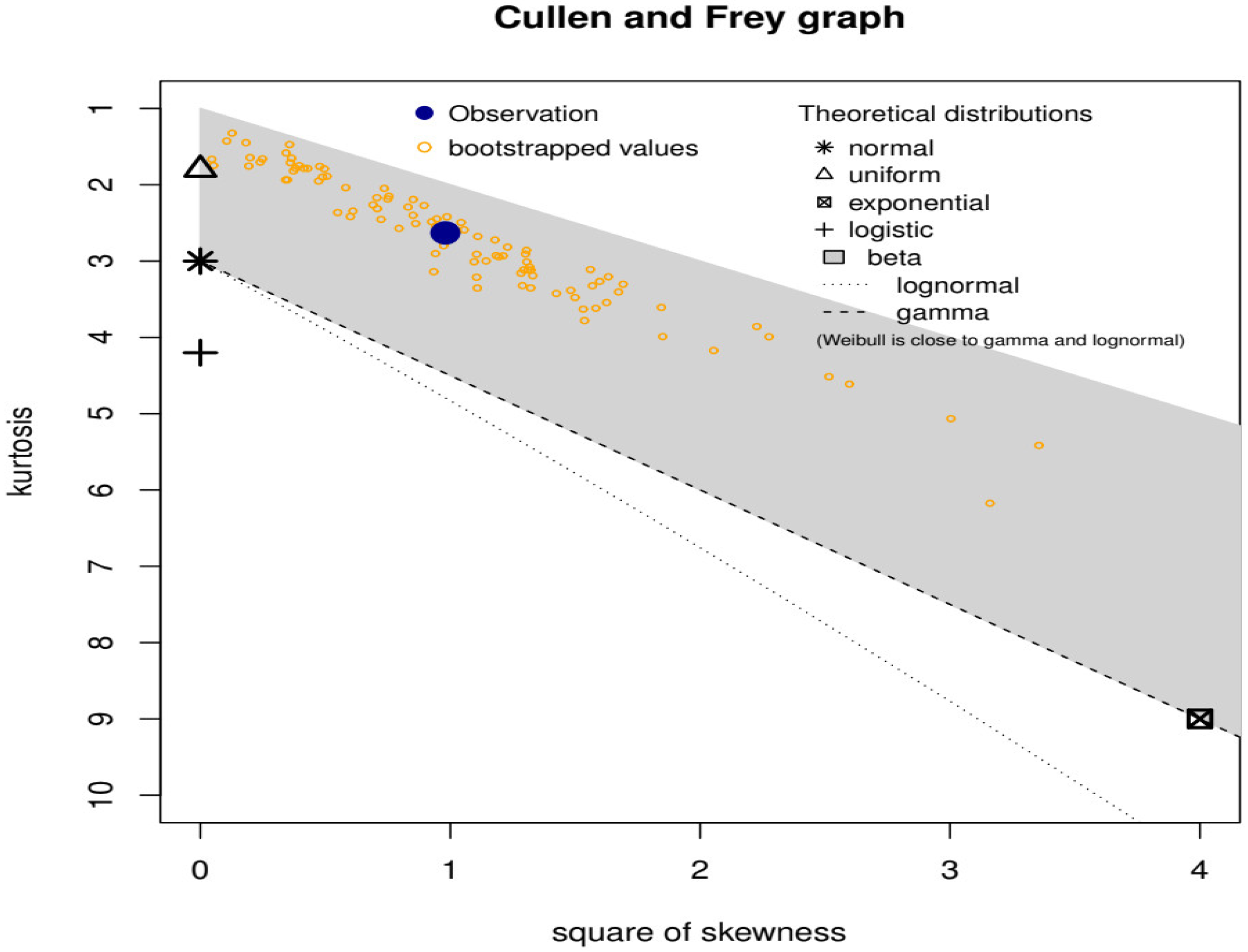
In addition to numerical research, graphical methods are employed to look at how theoretical distributions initially fit and how the densities of actuarial claims take shape. The Cullen and Frey plot helps identify whether a dataset deviates from a normal distribution. Understanding the distributional characteristics of data is crucial in many statistical analyses, as assumptions about normality often underlie many statistical tests. Skewness, which is represented on the x-axis of the plot, measures the extent to which the data distribution is asymmetric. Positive skewness indicates a longer right tail, while negative skewness suggests a longer left tail. The plot helps visualize and quantify the skewness of the dataset. Kurtosis, shown on the y-axis of the plot, measures the degree of peakedness or flatness of a distribution compared to a normal distribution. High positive kurtosis implies heavy tails, while negative kurtosis suggests lighter tails. Analyzing kurtosis helps us understand the presence of outliers or extreme values in the dataset. Figure 2 gives the Cullen and Frey plot for actuarial claims data. The Cullen and Frey (skewness–kurtosis plot) in Figure 2 reveals that the data are left-skewed with a kurtosis of less than 3. The big blue dot refers to our insurance data. It is clear that the data stay away from the main points which represent normal distribution and exponential distribution. Also, our insurance data are away from the lines which represent gamma distribution and lognormal distribution. By projecting vertically to those lines, we can see that the data have lower kurtosis than the lognormal and the gamma models of the same skewness.

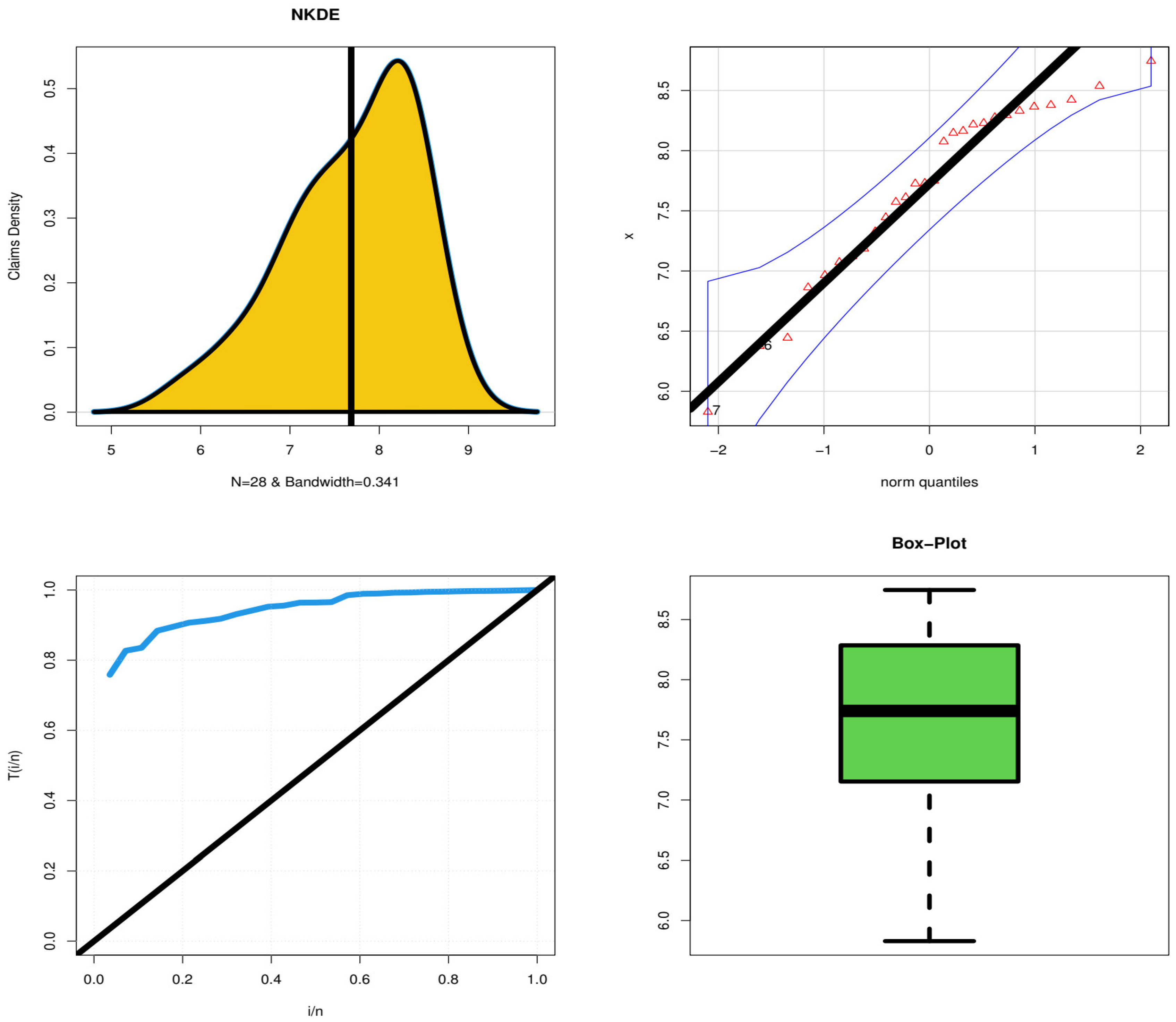
The nonparametric kernel density estimation (NKDE) method (top left), the quantile-quantile (Q-Q) plot (top right), the total time on test (TTT) plot (bottom left), and the “box plot” (bottom right) are only a few of the graphical techniques shown in Figure 3 below.

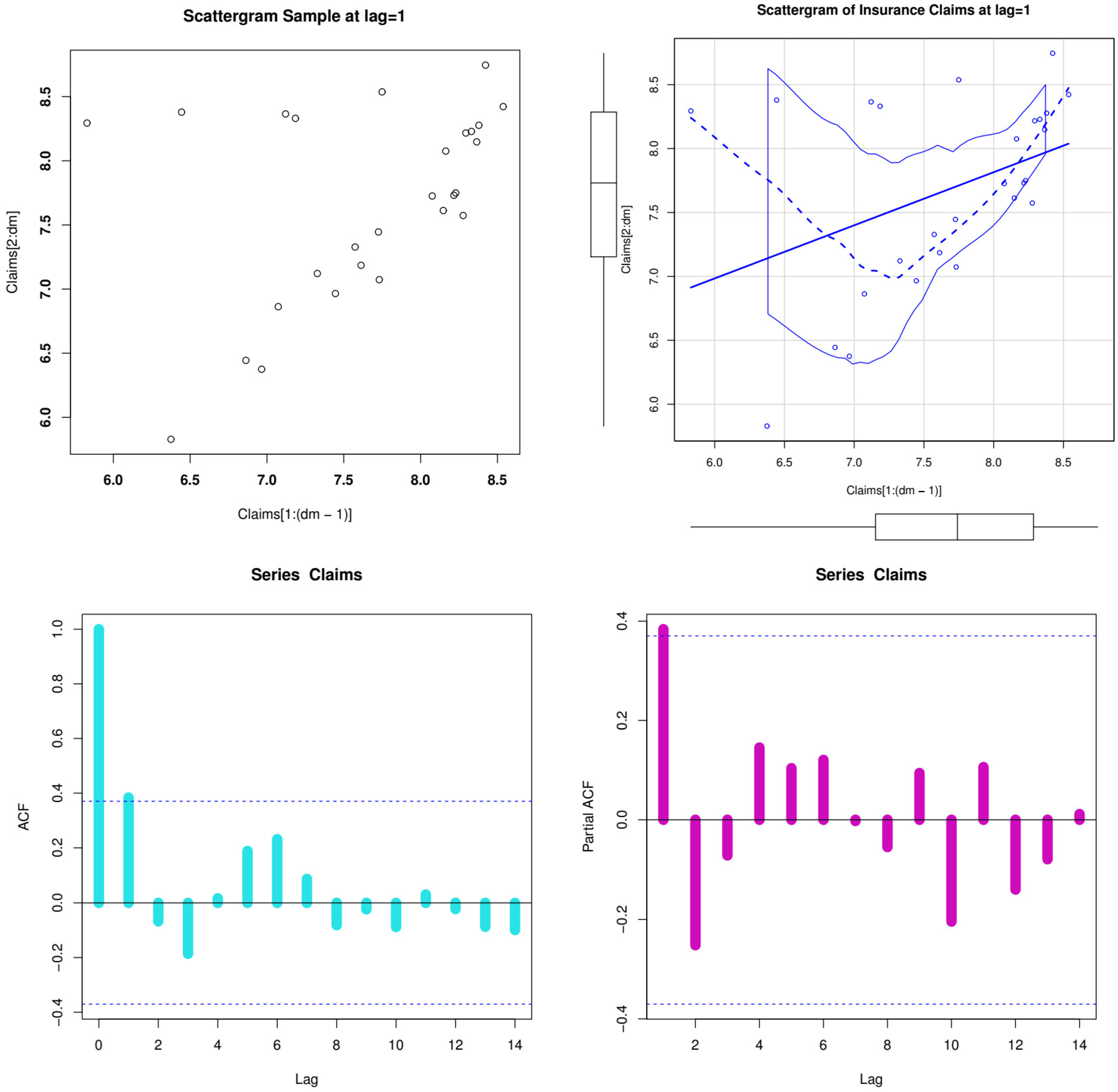
Figure 3 (top left panel) shows that the initial density is an asymmetric function with a left tail and that there are no extreme observations. Figure 3 (top right panel) shows that data do not contain any extreme values. According to the TTT plot (Figure 3 (bottom right panel)), the hazard rate function for the models used to explain the current data should be consistently growing. Figure 3 (bottom right panel) shows that the data do not contain any extreme values. The scattergrams for the data on actuarial claim size are shown in Figure 4 (first row panels), where Figure 4 (top left) refers to the initial scattergram and Figure 4 (top right) refers to the fitted scattergram. For the actuarial claim size data, the autocorrelation function (ACF) and partial autocorrelation function (partial-ACF) are shown in Figure 4’s second row. We offer the ACF, which can be used to demonstrate how the correlation between any two signal values alters when the distance between them alters the ACF.

The theoretical ACF is a time domain measure of the stochastic process memory and offers no insight into the frequency content of the process. Also included is the theoretical partial ACF with Lag = k = 1; see Figure 4 (bottom right panel). The initial lag value is statistically significant, while none of the other partial autocorrelations for any other delays are, according to Figure 4’s bottom right corner. This proposes an autoregressive (AR(1)) model as a potential fit to these data. Due to our data, skewness = −0.74828 (left-skewed data), kurtosis $=2.78846<$ 3, and dispersion index (DIx) $=0.070835$ (under dispersed data). Based on these Table 5 and Table 6, the following results can be highlighted:

• For all risk assessment methods:

$$\mathrm{For} \mathrm{GELX}: \mathrm{VaRK} \left(\mathcal{Z}{|}_{1-\mathcal{q}=0.3}\right)<\mathrm{VaRK} \left(\mathcal{Z}{|}_{1-\mathcal{q}=0.25}\right)<\dots <\mathrm{VaRK} \left(\mathcal{Z}{|}_{1-\mathcal{q}=0.1}\right)<\mathrm{VaRK} \left(\mathcal{Z}{|}_{1-\mathcal{q}=0.01}\right),$$

$$\mathrm{For} \mathrm{ELX}: \mathrm{VaRK} \left(\mathcal{Z}{|}_{1-\mathcal{q}=0.3}\right)<\mathrm{VaRK} \left(\mathcal{Z}{|}_{1-\mathcal{q}=0.25}\right)<\dots <\mathrm{VaRK} \left(\mathcal{Z}{|}_{1-\mathcal{q}=0.1}\right)<\mathrm{VaRK} \left(\mathcal{Z}{|}_{1-\mathcal{q}=0.01}\right).$$

2.

For all risk assessment methods:

$$\mathrm{For} \mathrm{GELX}: \mathrm{TVaRK}\left(\mathcal{Z}{|}_{1-\mathcal{q}=0.3}\right)<\mathrm{TVaRK}\left(\mathcal{Z}{|}_{1-\mathcal{q}=0.25}\right)<\dots <\mathrm{TVaRK}\left(\mathcal{Z}{|}_{1-\mathcal{q}=0.1}\right)<\mathrm{TVaRK}\left(\mathcal{Z}{|}_{1-\mathcal{q}=0.01}\right),$$

$$\mathrm{For} \mathrm{ELX}: \mathrm{TVaRK}\left(\mathcal{Z}{|}_{1-\mathcal{q}=0.3}\right)<\mathrm{TVaRK}\left(\mathcal{Z}{|}_{1-\mathcal{q}=0.25}\right)<\dots <\mathrm{TVaRK}\left(\mathcal{Z}{|}_{1-\mathcal{q}=0.1}\right)<\mathrm{TVaRK}\left(\mathcal{Z}{|}_{1-\mathcal{q}=0.01}\right).$$

3.

For all risk assessment methods:

$$\mathrm{For} \mathrm{GELX}: \mathrm{TV}\left(\mathcal{Z}{|}_{1-\mathcal{q}=0.3}\right)<\mathrm{TV}\left(\mathcal{Z}{|}_{1-\mathcal{q}=0.25}\right)<\dots <\mathrm{TV}\left(\mathcal{Z}{|}_{1-\mathcal{q}=0.1}\right)<\mathrm{TV}\left(\mathcal{Z}{|}_{1-\mathcal{q}=0.01}\right),$$

$$\mathrm{For} \mathrm{ELX}: \mathrm{TV}\left(\mathcal{Z}{|}_{1-\mathcal{q}=0.3}\right)>\mathrm{TV}\left(\mathcal{Z}{|}_{1-\mathcal{q}=0.25}\right)>\dots >\mathrm{TV}\left(\mathcal{Z}{|}_{1-\mathcal{q}=0.1}\right)>\mathrm{TV}\left(\mathcal{Z}{|}_{1-\mathcal{q}=0.01}\right).$$

4.

For all risk assessment methods:

$$\mathrm{For} \mathrm{GELX}: \mathrm{TMVK}\left(\mathcal{Z}{|}_{1-\mathcal{q}=0.3}\right)<\mathrm{TMVK}\left(\mathcal{Z}{|}_{1-\mathcal{q}=0.25}\right)<\dots <\mathrm{TMVK}\left(\mathcal{Z}{|}_{1-\mathcal{q}=0.1}\right)<\mathrm{TMVK}\left(\mathcal{Z}{|}_{1-\mathcal{q}=0.01}\right),$$

$$\mathrm{For} \mathrm{ELX}: \mathrm{TMVK}\left(\mathcal{Z}{|}_{1-\mathcal{q}=0.3}\right)>\mathrm{TMVK}\left(\mathcal{Z}{|}_{1-\mathcal{q}=0.25}\right)>\dots >\mathrm{TMVK}\left(\mathcal{Z}{|}_{1-\mathcal{q}=0.1}\right)>\mathrm{TMVK}\left(\mathcal{Z}{|}_{1-\mathcal{q}=0.01}\right).$$

5.

For all risk assessment methods:

$$\mathrm{For} \mathrm{GELX}: \mathrm{MELS}\left(\mathcal{Z}{|}_{1-\mathcal{q}=0.3}\right)<\mathrm{MELS}\left(\mathcal{Z}{|}_{1-\mathcal{q}=0.25}\right)<\dots <\mathrm{MELS}\left(\mathcal{Z}{|}_{1-\mathcal{q}=0.1}\right)<\mathrm{MELS}\left(\mathcal{Z}{|}_{1-\mathcal{q}=0.01}\right),$$

$$\mathrm{For} \mathrm{ELX}: \mathrm{MELS}\left(\mathcal{Z}{|}_{1-\mathcal{q}=0.3}\right)>\mathrm{MELS}\left(\mathcal{Z}{|}_{1-\mathcal{q}=0.25}\right)>\dots >\mathrm{MELS}\left(\mathcal{Z}{|}_{1-\mathcal{q}=0.1}\right)>\mathrm{MELS}\left(\mathcal{Z}{|}_{1-\mathcal{q}=0.01}\right).$$

6.

Under the MAXLE method and the GELX model: The VaRK$\left(\mathcal{Z}\right)$ is consistently growing, starting with 3104.32244 and ending with 12,791.47826; the TVaRK$\left(\mathcal{Z}\right)$ is consistently growing, starting with 5606.27701 and ending with 17,177.67141.

7.

Under the ORLSE method and the GELX model: The VaRK$\left(\mathcal{Z}\right)$ is consistently growing, starting with 3559.79706 and ending with 18,274.02938; the TVaRK$\left(\mathcal{Z}\right)$ is consistently growing, starting with 7134.33969 and ending with 26,462.60076.

8.

Under the L-MO method and the GELX model: The VaRK$\left(\mathcal{Z}\right)$ is consistently growing, starting with 2684.87356 and ending with 7251.04539; the TVaRK$\left(\mathcal{Z}\right)$ is consistently growing, starting with 3955.54267 and ending with 8938.81397.

9.

Under the ADE method and the GELX model: The VaRK$\left(\mathcal{Z}\right)$ is consistently growing, starting with 3428.17317 and ending with 14,714.50356; the TVaRK$\left(\mathcal{Z}\right)$ is consistently growing, starting with 6329.36348 and ending with 19,871.73902. Similarly, the TVq$\left(\mathcal{Z}\right)$, the $\mathrm{TMVK}\left(\mathcal{Z}\right),$ and the MEL$\left(\mathcal{Z}\right)$ are consistently growing. Under the ADE method and the ELX model: The VaRK is consistently growing, starting with 3440.462517 and ending with 11,119.778633; the TVaRK is consistently growing, starting with 5686.884025 and ending with 13,422.696625. However, the TVq, the TMVK, and the MEL are monotonically decreasing.

10.

For the GELX model: For nearly for all $\mathcal{q}$ values, the ORLSE method is recommended since it provides the most acceptable risk exposure analysis; then, the MAXLE method is recommended as a second one, then the ADE method, and then the L-MO method. However, the other two methods perform well. For the ELX model: For nearly for all $\mathcal{q}$ values, the ORLSE method is recommended since it provides the most acceptable risk exposure analysis; then, the MAXLE method is recommended as a second one. However, the other two methods also perform well.

6. Construction of RRNIK Statistic for the GELX Model

Many statistical tests assume that the data are normally distributed. If the data are skewed, these tests may not be appropriate and can lead to incorrect conclusions. By using a skewed distribution to model the data, more robust statistical tests can be used to test hypotheses and make inferences. Skewed distributions can be used to make better decisions in various fields, such as finance, insurance, and engineering. By accurately modeling the data and estimating the likelihood of extreme events, decisions can be made that are more informed and better account for risk.

The RRNIK statistic is a well-known substitute for the traditional chi-squared tests where there are complete data (for additional information, see Nikulin [8], Nikulin [9], Nikulin [10], and Rao and Robson [11]). The most popular test to check whether a mathematical model is suitable for the data from observations is the Pearson chi-square statistic. But in cases where the model’s parameters are unknown or the data are censored, these tests are useless. For the entire set of data, Nikulin [8], Nikulin [9], Nikulin [10], and Rao and Robson [11] all indicated natural variations in the Pearson statistic, which is referred to as RRNIK. The chi-square distribution, a logical extension of the Pearson statistic, is used in this statistical test.

When the filtering is applied on top of the unknown parameter, the standard test is not strong enough to establish the null hypothesis. Nikulin [8], Nikulin [9], Nikulin [10], and Rao and Robson [11] suggest that the RRNIK statistic be modified to take into consideration random right censoring. In the current study, we provide a modified chi-square test for the GELX model (see also Bagdonavičius et al. [29], Bagdonavičius and Nikulin [30], Bagdonavičius and Nikulin [31] for more details). To test the theory, Nikulin [8], Nikulin [9], Nikulin [10], and Rao and Robson [11] established the RRNIK statistic ${\mathcal{Y}}^2\left({\widehat{\underset{\_}{\mathcal{V}}}}_{\mathcal{m}}\right)$). Let

$$H_0\hspace{1em}\hspace{1em}:\hspace{1em}\hspace{1em}\stackrel{}{\mathrm{Pr}}\left\{{\mathcal{Z}}_{\underset{\_}{\mathcal{V}}}\le \mathcal{z}\right\}=F_{\underset{\_}{\mathcal{V}}}\left(\mathcal{z}\right){|}_{\mathcal{z}\in R}.$$

Then, according to Nikulin [8], Nikulin [9], Nikulin [10] and Rao and Robson [11], we have

$${\mathcal{Y}}^2\left({\widehat{\underset{\_}{\mathcal{V}}}}_{\mathcal{m}}\right)=Z_{\mathcal{m}}^2\left({\widehat{\underset{\_}{\mathcal{V}}}}_{\mathcal{m}}\right)+{\mathcal{m}}^{-1}{L}^T\left({\widehat{\underset{\_}{\mathcal{V}}}}_{\mathcal{m}}\right){\left({\rm I}\left({\widehat{\underset{\_}{\mathcal{V}}}}_{\mathcal{m}}\right)-J\left({\widehat{\underset{\_}{\mathcal{V}}}}_{\mathcal{m}}\right)\right)}^{-1}L\left({\widehat{\underset{\_}{\mathcal{V}}}}_{\mathcal{m}}\right),$$

where

$$Z_{\mathcal{m}}^2\left({\widehat{\underset{\_}{\mathcal{V}}}}_{\mathcal{m}}\right)={\left(\frac{{\varsigma }_1-\mathcal{m}{p}_1\left({\widehat{\underset{\_}{\mathcal{V}}}}_{\mathcal{m}}\right)}{\sqrt{\mathcal{m}{p}_1\left({\widehat{\underset{\_}{\mathcal{V}}}}_{\mathcal{m}}\right)}},\frac{{\varsigma }_2-\mathcal{m}{p}_2\left({\widehat{\underset{\_}{\mathcal{V}}}}_{\mathcal{m}}\right)}{\sqrt{\mathcal{m}{p}_2\left({\widehat{\underset{\_}{\mathcal{V}}}}_{\mathcal{m}}\right)}},\cdots ,\frac{{\varsigma }_{\mathcal{m}}-\mathcal{m}{p}_b\left({\widehat{\underset{\_}{\mathcal{V}}}}_{\mathcal{m}}\right)}{\sqrt{\mathcal{m}{p}_b\left({\widehat{\underset{\_}{\mathcal{V}}}}_{\mathcal{m}}\right)}}\right)}^T$$

and $J\left({\widehat{\underset{\_}{\mathcal{V}}}}_{\mathcal{m}}\right)$ is the information matrix for the grouped data

$$J\left({\widehat{\underset{\_}{\mathcal{V}}}}_{\mathcal{m}}\right)=ℬ{\left({\widehat{\underset{\_}{\mathcal{V}}}}_{\mathcal{m}}\right)}^Tℬ\left({\widehat{\underset{\_}{\mathcal{V}}}}_{\mathcal{m}}\right),$$

with

$$ℬ\left({\widehat{\underset{\_}{\mathcal{V}}}}_{\mathcal{m}}\right)={\left[\frac{1}{{\sqrt{p}}_{\mathcal{i}}}\frac{\partial }{\partial {\widehat{\underset{\_}{\mathcal{V}}}}_{\mathcal{m}}}{p}_{\mathcal{i}}\left({\widehat{\underset{\_}{\mathcal{V}}}}_{\mathcal{m}}\right)\right]}_{\mathcal{r}\times s}{|}_{\left(\mathcal{i}=1,2,\cdots ,b\hspace{1em}and k=1,2,\cdots ,s\right)},$$

and then

$$L\left({\widehat{\underset{\_}{\mathcal{V}}}}_{\mathcal{m}}\right)={\left(L_1\left({\widehat{\underset{\_}{\mathcal{V}}}}_{\mathcal{m}}\right),\dots ,L_s\left({\widehat{\underset{\_}{\mathcal{V}}}}_{\mathcal{m}}\right)\right)}^T\hspace{1em}\mathrm{with}\hspace{1em}{\mathrm{L}}_k\left({\widehat{\underset{\_}{\mathcal{V}}}}_{\mathcal{m}}\right)={\displaystyle \sum }_{\mathcal{i}=1}^{\mathcal{r}}\frac{{\varsigma }_{\mathcal{i}}}{p_{\mathcal{i}}}\frac{\partial }{\partial \left({\widehat{\underset{\_}{\mathcal{V}}}}_{\mathcal{m}}\right)}{p}_{\mathcal{i}}\left({\widehat{\underset{\_}{\mathcal{V}}}}_{\mathcal{m}}\right),$$

where $\widehat{I}$ refers to the estimated Fisher INFMX. Then, the ${\mathcal{Y}}^2$ statistic has $\left(b-1\right)$ degrees of freedom (DOF), and it follows the Chi square model. Consider a set of observations that are divided into $I_1,I_2,\cdots ,I_b$, where

$$I_j=\left({\mathcal{A}}_{j,b}\left(\mathcal{z}\right)-1;{\mathcal{A}}_{j,b}\left(\mathcal{z}\right)\right)$$

$$p_j\left(\underset{\_}{\mathcal{V}}\right)={{\displaystyle \int }}_{{\mathcal{A}}_{j,b}\left(\mathcal{z}\right)-1}^{{\mathcal{A}}_{j,b}\left(\mathcal{z}\right)}{f}_{\underset{\_}{\mathcal{V}}}\left(\mathcal{z}\right)d\mathcal{z}{|}_{\left(j=1,2,\cdots ,b\right)},$$

and

$${\mathcal{A}}_{j,b}\left(\mathcal{z}\right)=F^{-1}\left(\frac{j}{b}\right){|}_{\left(j=1,\cdots ,b-1\right)}.$$

In this research, we create a modified goodness-of-fit test known as the RRNIK statistic to examine if the used data follow the distribution of the GELX model when a parameter is unknown. Our new statistic relies on the estimated Fisher INFMX, which we employ after computing the highest likelihood estimator of the unknown GELX distribution parameter on the dataset.

7. Uncensored Distributional Validation

To test a hypothesis with censored data and an unknown parameter, we utilize a specific type of statistical test based on the RRNIK statistic variation, as suggested by Nikulin [7,8,9] and Rao and Robson [11]. Our adaptation of this test is tailored for the GELX model, where the failure rate ${\mathcal{z}}_i$ follows a GELX distribution. The null hypothesis is then considered:

$$H_0:F\left(\mathcal{z}\right)\in F_0=F_{0,\underset{\_}{\mathcal{V}}}\left(\mathcal{z}\right){|}_{\mathcal{z}\in R}.$$

Below are the expressions for the survival function (SrF) and cumulative hazard function of the GELX distribution:

$$S_{\underset{\_}{\mathcal{V}}}\left(\mathcal{z}\right)=1-F_{\underset{\_}{\mathcal{V}}}\left(\mathcal{z}\right)=1-{\left[1-exp\left\{-{\left[{\psi }_{{\delta }_2,\beta }\left(z\right)-1\right]}^{-1}\right\}\right]}^{{\delta }_1}{|}_{\underset{\_}{\mathcal{V}}={\delta }_1,{\delta }_2,\beta },$$

and

$${\mathit{V}}_{\underset{\_}{\mathcal{V}}}\left(\mathcal{z}\right)=-\ln \left[S_{\underset{\_}{\mathcal{V}}}\left(\mathcal{z}\right)\right],$$

For all $j$, we have a constant value of $e_{j,\mathcal{Z}}=E_k/k$, where

$$E_{\mathit{k}}=E_{\mathit{k}}\left(\mathcal{z}\right)={{\displaystyle \sum }}_{l=1}^{\mathcal{i}-1}{\mathit{V}}_{\underset{\_}{\mathcal{V}}}\left(\mathcal{z}\right)|0=<{\mathcal{A}}_{0,b}<{\mathcal{A}}_{1,b}<\dots <{\mathcal{A}}_{k-1,b}<{\mathcal{A}}_{k,b}=+\infty .,$$

and ${\mathcal{A}}_{j,b}\left(\mathcal{z}\right)$ are random data functions. Then, the test statistic can be formulated as

$${\mathcal{Y}}_{\mathcal{m},\mathcal{r}-1,\mathcal{q}}^2\left(\widehat{\underset{\_}{\mathcal{V}}}\right)=Z^T\widehat{S^{-}}Z|Z={(Z_1,Z_2,\dots ,Z_k)}^T$$

where

$$Z_j=\frac{1}{\sqrt{\mathcal{m}}}\left({\mathcal{Q}}_{j,\mathcal{Z}}-e_{j,\mathcal{Z}}\right){|}_{\left(\hspace{1em}j=1,2,\dots ,k\right)}.$$

Then, the test statistic can also be presented in the following formula:

$${\mathcal{Y}}_{\mathcal{m},\mathcal{r}-1,\mathcal{q}}^2\left(\widehat{\underset{\_}{\mathcal{V}}}\right)={\displaystyle \sum }_{j=1}^k\frac{1}{{\mathcal{Q}}_{j,\mathcal{Z}}}{({\mathcal{Q}}_{j,\mathcal{Z}}-e_{j,\mathcal{Z}})}^2+{\mathit{V}}_{W,G},$$

where ${\mathit{V}}_{W,G}$ and many other details are given in Nikulin [8], Nikulin [9], Nikulin [10], and Rao and Robson [11].

7.1. Uncensored Simulation Study and Assessment under the RRNIK Statistics ${\mathcal{Y}}^2\left(\mathcal{q};\widehat{\underset{\_}{\mathcal{V}}}\right)$

Here are some general steps to conduct a simulation study using the Rao–Robson Nikulin test statistic:

I.

Define the GELX distribution by specifying its parameters, such as the location, scale, and shape parameters.

II.

Set the sample size and the censoring mechanism. For instance, you can choose a fixed sample size and right-censor the data at a certain time point.

III.

Generate multiple sets of simulated data from the GELX distribution with the specified parameters and censoring mechanism. The number of simulated datasets should be sufficiently large to obtain reliable results.

IV.

For each simulated dataset, estimate the GELX parameters using maximum likelihood estimation or another appropriate method.

V.

Compute the Rao-Robson Nikulin test statistic for each simulated dataset using the estimated parameters and the censoring information.

VI.

Calculate the empirical distribution of the test statistic across all simulated datasets.

VII.

Compare the observed test statistic from the actual data with the empirical distribution obtained from the simulation study. Evaluate whether the observed test statistic falls within the expected range under the null hypothesis or not.

Repeat steps III–VII for different sets of GELX parameters, sample sizes, and censoring mechanisms to assess the performance of the test statistic under various scenarios. Then,

Table 7. Empirical levels and corresponding theoretical levels ($\mathcal{q}$ = 0.01, 0.02, 0.05, and 0.1) and N = 16,000.

$\mathit{m}$  $\downarrow \mathbf{and} \mathcal{q}\to$	${\mathcal{q}}_1$ = 0.01	${\mathcal{q}}_2$ = 0.02	${\mathcal{q}}_3$ = 0.05	${\mathcal{q}}_4$ = 0.1
${\mathcal{m}}_1=25$	0.9935	0.9819	0.9522	0.9033
${\mathcal{m}}_2=40$	0.9929	0.9817	0.9515	0.9025
${\mathcal{m}}_3=150$	0.9922	0.9811	0.9509	0.9017
${\mathcal{m}}_5=300$	0.9911	0.9807	0.9506	0.9010
${\mathcal{m}}_6=700$	0.9906	0.9805	0.9503	0.9003

shows the relevant empirical and theoretical levels. It is clear that the determined empirical level value and its equivalent theoretical level value are fairly similar. As a result, we draw the conclusion that the suggested test is excellent for the GELX distribution.

7.2. Uncensored Reliability Data Modeling and Testing under the RRNIK Statistics ${\mathcal{Y}}^2\left(\mathcal{q};\widehat{\underset{\_}{\mathcal{V}}}\right)$

7.2.1. Uncensored Reliability Strength’s Dataset

To model the uncensored reliability strengths dataset using a probability distribution, one commonly used distribution is the Weibull distribution. The Weibull distribution is frequently employed in reliability analyses due to its flexibility in capturing a wide range of failure patterns. In this application, we test the GELX distribution for the uncensored reliability strengths dataset. Using the BB algorithm (see Ravi (2009)) and the reliability data of Nichols and Padgett [32], we can obtain the MAXLE value of the parameter $\delta ,$ assuming that our GELX model can fit the strength data of $1.5$ cm glass fiber: $\widehat{{\delta }_1}=1.52493, \widehat{{\delta }_2}=1.99834,\widehat{\beta }=0.73854$. We can compute and provide the Fisher INFMX as follows using the value:

$$I\left(\widehat{\underset{\_}{\mathcal{V}}}\right)=\left[\begin{array}{ccc}0.953428& 1.26758& 2.139537\\ & 2.10348& 4.801254\\ & & 0.996598\end{array}\right]$$

Then, ${\mathcal{Y}}^2\left(\mathcal{q};\widehat{\underset{\_}{\mathcal{V}}}\right)=12.004875$ and the critical value ${\chi }_{0.05}^2\left(6\right)=12.5916$, which means that the GELX distribution can effectively express, simulate, and model the uncensored reliability strength’s dataset. However, selecting the appropriate distribution necessitates evaluating the data’s fit to each distribution, usually through the use of statistical tests or a visual examination of the data plotted against the selected distribution. The selection procedure may also be aided by domain expertise and theoretical factors.

7.2.2. Uncensored Heat Exchanger Tube Crack

To model the uncensored heat exchanger tube crack dataset using a probability distribution, you need to determine the appropriate distribution that best fits the data. The choice of distribution depends on the characteristics of the dataset and the underlying assumptions you wish to make. Following the BB algorithm and using the data of Meeker and Escobar [33], we are concerned with testing the null hypothesis that the heat exchanger tube crack data follow our GELX distribution under the RRNIK statistic test. First, we have the MAXLE for the three parameters, where $\widehat{{\delta }_1}=3.12542,\widehat{{\delta }_2}=2.73154,\widehat{\beta }=0.83496$. Second, the INFMX can be obtained as

$$I\left(\widehat{\underset{\_}{\mathcal{V}}}\right)=\left[\begin{array}{ccc}0.437812& 3.76831& 1.00703\\ & 1.76948& 5.11147\\ & & 1.354706\end{array}\right]$$

Then, we also have the following main results: ${\mathcal{Y}}^2\left(\mathcal{q};\widehat{\underset{\_}{\mathcal{V}}}\right)=19.60143$ and ${\chi }_{0.01}^2\left(12\right)=21.02607$, which means that the GELX distribution can effectively express, simulate, and model the uncensored heat exchanger tube crack dataset. However, choosing the best distribution involves assessing the fit of the data to each distribution, typically by using statistical tests or visual inspection of the data plotted against the chosen distribution. Additionally, domain knowledge and theoretical considerations can help guide the selection process.

8. Censored Distributional Validation

8.1. Censored Simulation Study and Assessment under the RRNIK Statistics ${\mathcal{Y}}_{n,\mathcal{r}-1,\mathcal{q}}^2\left(\widehat{\underset{\_}{\mathcal{V}}}\right)$

A censored simulation study under the Rao–Robson Nikulin (RRNIK) statistics is a method for testing the goodness of fit of a censored distribution using simulated data. This method is based on the RRNIK test statistic, which is a variation of the Kolmogorov–Smirnov test statistic that takes into account the censoring of the data. To perform a censored simulation study using the RRNIK statistics, the first step is to generate a set of simulated data with known distribution parameters. The data should be generated in such a way that it contains a mixture of censored and uncensored data. This can be achieved by randomly censoring a portion of the data or by using a censoring mechanism that is appropriate for the application. Once the simulated data are generated, the RRNIK test statistic can be calculated by comparing the empirical distribution function of the censored data to the hypothesized distribution function. The test statistic is then compared to a critical value from a distribution table to determine whether the null hypothesis can be rejected. The null hypothesis is that the censored data comes from the hypothesized distribution function. The censored simulation study can be repeated multiple times with different sets of simulated data to obtain a more accurate assessment of the goodness of fit of the hypothesized distribution to the observed data. This can help to determine the robustness of the RRNIK test statistic and its ability to accurately detect deviations from the hypothesized distribution. Overall, censored simulation studies using the RRNIK statistics are a useful tool for assessing the performance of the RRNIK test statistic in detecting deviations from the hypothesized distribution in censored data. This method can be applied in a variety of applications, including reliability analysis, survival analysis, and the modeling of extreme events.

Under the censored simulated studies, the RRNIK statistics ${\mathcal{Y}}_{\mathcal{m},\mathcal{r}-1,\mathcal{q}}^2\left(\widehat{\underset{\_}{\mathcal{V}}}\right)$ can be evaluated with some experiments. For N = 17,000 samples and censoring at $25\%$ with $\mathrm{DOF}=5$, we can calculate the average value of the non-rejection numbers of the null hypothesis for $\mathcal{q}=0.01, 0.02, 0.05, 0.1$, where ${\mathcal{Y}}_{\mathcal{m},\mathcal{r}-1,\mathcal{q}}^2\left(\widehat{\underset{\_}{\mathcal{V}}}\right)\le$ ${\chi }_{\mathcal{q}}^2\left(\mathcal{r}-1\right)$. The simulation results are presented in

Table 8. Censored simulation study and assessment under the RRNIK. Statistics for $\mathcal{q}=0.01, 0.02, 0.05, \mathrm{and} 0.1$ and N = 17,000.

$\mathit{m}$  $\downarrow \mathbf{and} \mathcal{q}\to$	${\mathcal{q}}_1$ = 0.01	${\mathcal{q}}_2$ = 0.02	${\mathcal{q}}_3$ = 0.05	${\mathcal{q}}_4$ = 0.1
${\mathcal{m}}_1=25$	0.9924	0.9831	0.9522	0.9029
${\mathcal{m}}_2=40$	0.9920	0.9822	0.9515	0.9019
${\mathcal{m}}_3=150$	0.9911	0.9818	0.9510	0.9009
${\mathcal{m}}_5=300$	0.9908	0.9809	0.9505	0.9003
${\mathcal{m}}_6=700$	0.9905	0.9804	0.9502	0.9002

.

8.2. Right Censored Medical and Reliability Datasets under the RRNIK Statistics ${\mathcal{Y}}_{n,\mathcal{r}-1,\mathcal{q}}^2\left(\widehat{\underset{\_}{\mathcal{V}}}\right)$

8.2.1. Right Censored Medical Lung Cancer Dataset

The censored lung cancer dataset (see Loprinzi et al. [34]) is a valuable resource for researchers interested in developing and testing statistical models for survival data, as well as for clinicians and policymakers interested in understanding the factors that contribute to survival outcomes for patients with lung cancer, where $\mathcal{m}=228$ and right censored items $=63$. First, we have the following results: $\widehat{{\delta }_1}=1.93548,\widehat{{\delta }_2}=1.44046,\widehat{\beta }=0.69421$. As a number of classes, we employ DOF $=8$. The following results refer to how the test statistic ${\mathcal{Y}}_{\mathcal{m},\mathcal{r}-1,\mathcal{q}}^2\left(\widehat{\underset{\_}{\mathcal{V}}}\right)$ items are presented:

$\widehat{{\mathcal{A}}_{j,b}\left(\mathcal{Z}\right)}$	92.14	171.69	216.04	283.0	355.10	456.30	685.30	1022.32
$\widehat{{\mathcal{Q}}_{j,\mathcal{Z}}}$	29.0	30.0	35.0	31.0	32.0	25.0	28.0	18.0
$e_{j,\mathcal{Z}}$	8.27173	8.27173	8.27173	8.27173	8.27173	8.27173	8.27173	8.27173

Then, the estimated matrix $\widehat{P_{\mathcal{i}\mathcal{j}}}\left(\mathcal{Z}\right)$ are as follows:

$\widehat{P_{1\mathcal{j}}}\left(\mathcal{Z}\right)$	−0.5674	0.8437	−0.7391	0.1637	0.9000	0.7064	−0.2061	0.2836
$\widehat{P_{1\mathcal{j}}}\left(\mathcal{Z}\right)$	0.7168	−0.1834	0.8245	0.7601	0.3761	0.3066	0.7004	0.2994
$\widehat{P_{1\mathcal{j}}}\left(\mathcal{Z}\right)$	0.6974	−0.8312	0.6498	0.8526	0.5084	0.0942	0.6474	0.1991

and

$$I\left(\widehat{\underset{\_}{\mathcal{V}}}\right)=\left[\begin{array}{ccc}0.86451& 1.62348& 2.49312\\ & 0.75550& 5.11147\\ & & 0.93784\end{array}\right].$$

The critical value of ${\chi }_{0.05}^2\left(\mathrm{DOF}=8\right)=15.50731$, whereas ${\mathcal{Y}}_{\mathcal{m},\mathcal{r}-1,\mathcal{q}}^2\left(\widehat{\underset{\_}{\mathcal{V}}}\right)=12.95384$, which means that the GELX distribution can effectively express, simulate, and model the censored medical lung cancer dataset.

8.2.2. Right Censored Reliability Dataset

The censored reliability dataset is an excellent resource for researchers who are interested in developing and testing statistical models for time-to-failure data. These researchers can obtain the dataset on the Internet. The filtered reliability dataset is an extremely helpful resource for engineers and manufacturers who are interested in improving the dependability of the goods or systems they produce. A set of data for basic reliability assessments, obtained from an experiment with several factors, includes data on the lifetime of glass capacitors as a function of voltage and operating temperature. The dataset includes data on the longevity of glass capacitors as a function of voltage and operating temperature (see Meeker and Escobar [33]). Consider the data of Meeker and Escobar [33], where $\mathcal{m}=64$ and right censored items $=32$. Then, we have: $\widehat{{\delta }_1}=2.1473,\widehat{{\delta }_2}=1.3614,\widehat{\beta }=0.83760$. Considering DOF $= 8$, we gain the following results:

$\widehat{{\mathcal{A}}_{j,b}\left(\mathcal{Z}\right)}$	346.16	469.50	587.11	679.02	1078.83	1089.11	1102.17	1106.44
$\widehat{{\mathcal{Q}}_{j,\mathcal{Z}}}$	11.0	15.0	6.0	10.0	6.0	5.0	6.0	5.0
$e_{j,\mathcal{Z}}$	3.6762	3.6762	3.6762	3.6762	3.6762	3.6762	3.6762	3.6762

Then, the estimated matrix  $\widehat{P_{\mathcal{i}\mathcal{j}}}\left(\mathcal{Z}\right)$ are as follows:

$\widehat{P_{1\mathcal{j}}}\left(\mathcal{Z}\right)$	0.3674	0.9005	−0.6118	0.1667	0.7100	−0.6008	0.7487	0.6791
$\widehat{P_{1\mathcal{j}}}\left(\mathcal{Z}\right)$	0.3914	0.4351	0.7003	−0.3332	0.3846	0.3917	0.7066	0.2994
$\widehat{P_{1\mathcal{j}}}\left(\mathcal{Z}\right)$	0.6947	0.8668	0.1979	0.2852	0.4937	0.0971	−0.4444	0.1985

and

$$I\left(\widehat{\underset{\_}{\mathcal{V}}}\right)=\left[\begin{array}{ccc}0.49382& 4.0006& 2.35623\\ & 1.67940& 0.48163\\ & & 0.77185\end{array}\right].$$

Then, sine ${\mathcal{Y}}_{\mathcal{m},\mathcal{r}-1,\mathcal{q}}^2\left(\widehat{\underset{\_}{\mathcal{V}}}\right)=14.882811$ and ${\chi }_{0.05}^2\left(8\right)=15.50731$, which means that the GELX distribution can effectively express, simulate, and model the censored reliability dataset.

9. Validation for the Actuarial Data

The RRNIK test statistic is an essential tool that can be of service to researchers in the design of improved models and in the generation of more accurate forecasts. The validation of actuarial data using this test statistic is a critical instrument that can be of assistance to researchers. The validation of data using this test statistic is an important tool to have at your disposal when conducting an examination of actuarial data. The validation findings will be presented in accordance with the revised RRNIK statistical test in this section of the article. On the other hand, we are going to make use of the actuarial claims data this time around. In the event that our GELX model is able to produce a satisfactory match with the actuarial claims data, then we will be able to make use of the BB approach to obtain the MAXLE value of the parameters. This assumes that the MAXLE value can be calculated with a high degree of precision; then, we have $\widehat{{\delta }_1}=2.19046,\widehat{{\delta }_2}=0.93875, \widehat{\beta }=0.84755$. We can compute and provide the Fisher INFMX as follows using the value:

$$I\left(\widehat{\underset{\_}{\mathcal{V}}}\right)=\left[\begin{array}{ccc}0.89317& 2.30159& 4.12578\\ & 3.95148& 5.601474\\ & & 1.689457\end{array}\right].$$

The critical values for the RRNIK statistical test were ${\mathit{Y}}^2\left(\epsilon ;\widehat{\underset{\_}{\mathcal{V}}}\right)=9.843197$ and ${\chi }_{0.05}^2\left(5\right)=11.070$, so the GELX distribution can effectively simulate and model the actuarial claims data.

10. Concluding Remarks

In this paper, we introduce a new model for actuarial claims analysis and actuarial risk assessment. The risk assessment process was carried out through four different classical assessment methods: the maximum likelihood estimation (MAXLE), ordinary least squares (OLS), L-Moment (L-MO), and Anderson Darling estimation (ADE) methods. The risk exposure under actuarial claims data was also described using five important risk indicators: value-at-risk (VaRK$\left(\mathcal{Z}\right)$), tail-value-at-risk (TVaRK$\left(\mathcal{Z}\right)$), tail variance (TVq$\left(\mathcal{Z}\right)$), tail mean-variance ($\mathrm{TMVK}\left(\mathcal{Z}\right)$), and mean excess loss ($\mathrm{MELS}\left(\mathcal{Z}\right)$). These metrics were developed for the proposed weighted exponential model. The utilization of actuarial claims data in accordance with the five individual risk indicators is necessary in order to carry out an appropriate risk assessment. We came to the opinion that studying the actuarial claims data that fall within the five major risk indicators would be the most fruitful course of action given that the data have a distinct peak and a tail that progresses in a leftwards and unambiguous fashion. This led us to the conclusion that the best line of action would be to examine the facts. We felt compelled to provide both a numerical and graphical risk evaluation and analysis because the new distribution was able to model the data under a variety of different risk factors. This was because the new distribution was flexible enough to model the actuarial claims data under a variety of different risk indicators. This was mostly the cause of this. This was the main factor that motivated us to put out the effort. The fact that the properties of the new distribution matched those of the actuarial claims data sparked our interest in doing this study even more. We therefore determined that we ought to go and carry it out.

The following results can be highlighted:

• Under the artificial claims data: VaRK$\left(\mathcal{Z}\right)$, TVaRK$\left(\mathcal{Z}\right)$, TVq$\left(\mathcal{Z}\right)$, $\mathrm{TMVK}\left(\mathcal{Z}\right),$ and $\mathrm{MELS}\left(\mathcal{Z}\right)$ increase when $\mathcal{q}$ increases for all estimation methods.
• Under the artificial claims data:
  VaRK${\left(\mathcal{Z}\right)}_{MAXLE}<$ VaRK${\left(\mathcal{Z}\right)}_{ORLSE}<$ VaRK${\left(\mathcal{Z}\right)}_{ADE}<$ VaRK${\left(\mathcal{Z}\right)}_{L-MO}$ for most $\mathcal{q}$.
• Under the actuarial claims data, the MAXLE method, and the proposed model: The VaRK$\left(\mathcal{Z}\right)$, TVaRK$\left(\mathcal{Z}\right)$, TVq$\left(\mathcal{Z}\right)$, the $\mathrm{TMVK}\left(\mathcal{Z}\right),$ and the MEL$\left(\mathcal{Z}\right)$ are consistently growing.
• Under the actuarial claims data, the ORLSE method, and the proposed model: The VaRK$\left(\mathcal{Z}\right)$, TVaRK$\left(\mathcal{Z}\right)$, TVq$\left(\mathcal{Z}\right)$, the $\mathrm{TMVK}\left(\mathcal{Z}\right),$ and the MEL$\left(\mathcal{Z}\right)$ are consistently growing.
• Under the actuarial claims data, the L-MO method, and the proposed model: The VaRK$\left(\mathcal{Z}\right)$, TVaRK$\left(\mathcal{Z}\right)$, TVq$\left(\mathcal{Z}\right)$, the $\mathrm{TMVK}\left(\mathcal{Z}\right),$ and the MEL$\left(\mathcal{Z}\right)$ are consistently growing.
• Under the actuarial claims data, the ADE method, and the proposed model: The VaRK$\left(\mathcal{Z}\right)$, TVaRK$\left(\mathcal{Z}\right)$, TVq$\left(\mathcal{Z}\right)$, the $\mathrm{TMVK}\left(\mathcal{Z}\right),$ and the MEL$\left(\mathcal{Z}\right)$ are consistently growing.
• The ORLSE technique is strongly recommended for use with the new model as it provides the most dependable risk exposure analysis available. The MAXLE approach comes in a close second in the order of operations that have been proposed, followed by the ADE method, and finally, the L-MO method completes the series. On the other hand, the other two options are both successful in their own right and in their own particular way. Because it provides the most gratifying risk exposure analysis, the ORLSE methodology should be used for the ELX model. It is recommended to use this methodology. This is due to the fact that the ORLSE methodology delivers. As an alternative recommendation for a backup strategy, the MAXLE approach is the one that should be employed instead. On the other hand, the other two options are both successful in their own right and in their own particular way.
• For the testing and validation of the uncensored strengths of glass fibers data, the critical values for the RRNIK statistical test were ${\mathcal{Y}}^2\left(\mathcal{q};\widehat{\underset{\_}{\mathcal{V}}}\right)=12.004875$ and ${\chi }_{0.05}^2\left(6\right)=12.5916$; therefore, the new GELX distribution can effectively simulate and model the uncensored $1.5$ cm glass fiber data.
• For the testing and validation of the uncensored heat exchanger tube crack data, the critical values for the RRNIK statistical test were ${\mathcal{Y}}^2\left(\mathcal{q};\widehat{\underset{\_}{\mathcal{V}}}\right)=19.60143$ and ${\chi }_{0.05}^2\left(6\right)=12.5916$. As a result, the uncensored heat exchanger tube fracture data can be efficiently simulated and modelled using the new GELX distribution.
• For the testing and validation of the censored lung cancer dataset, the value of the statistical test ${\mathcal{Y}}_{\mathcal{m},\mathcal{r}-1,\mathcal{q}}^2\left(\widehat{\underset{\_}{\mathcal{V}}}\right)=12.95384$, where ${\chi }_{0.05}^2\left(8\right)=15.50731>{\mathcal{Y}}_{\mathcal{m},\mathcal{r}-1,\mathcal{q}}^2\left(\widehat{\underset{\_}{\mathcal{V}}}\right)=14.61654$. Consequently, the censored lung cancer dataset may be modeled using the new GELX model.
• For the testing and validation of the censored reliability dataset, the value of the statistical test ${\mathcal{Y}}_{\mathcal{m},\mathcal{r}-1,\mathcal{q}}^2\left(\widehat{\underset{\_}{\mathcal{V}}}\right)=13.84577$, where ${\chi }_{0.05}^2\left(8\right)=15.50731>{\mathcal{Y}}_{\mathcal{m},\mathcal{r}-1,\mathcal{q}}^2\left(\widehat{\underset{\_}{\mathcal{V}}}\right)=14.882811$. Therefore, the censored capacitor data reliability dataset may be modelled using the new GELX model.

References

1. Aboraya, M.; Ali, M.M.; Yousof, H.M.; Ibrahim, M. A novel Lomax extension with statistical properties, copulas, different estimation methods and applications. Bull. Malays. Math. Sci. Soc. 2022, 45, 85–120. [Google Scholar] [CrossRef]
2. Acerbi, C.; Tasche, D. On the coherence of expected shortfall. J. Bank. Financ. 2002, 26, 1487–1503. [Google Scholar] [CrossRef] [Green Version]
3. Adcock, C.; Eling, M.; Loperfido, N. Skewed distributions in finance and actuarial science: A review. Eur. J. Financ. 2015, 21, 1253–1281. [Google Scholar] [CrossRef]
4. Eling, M. Fitting insurance claims to skewed distributions: Are the skew-normal and skew-student good models? Insur. Math. Econ. 2012, 51, 239–248. [Google Scholar] [CrossRef]
5. Ali, M.M.; Korkmaz, M.Ç.; Yousof, H.M.; Butt, N.S. Odd Lindley-Lomax model: Statistical properties and applications. Pak. J. Stat. Oper. Res. 2019, 15, 419–430. [Google Scholar] [CrossRef]
6. Ali, M.M.; Yousof, H.M.; Ibrahim, M. A new Lomax type distribution: Properties, copulas, applications, Bayesian and non-Bayesian estimation methods. Int. J. Stat. Sci. 2021, 21, 61–104. [Google Scholar]
7. Alizadeh, M.; Ghosh, I.; Yousof, H.M.; Rasekhi, M.; Hamedani, G.G. The generalized odd-generalized exponential family of distributions: Properties, characterizations and applications. J. Data Sci. 2017, 15, 443–466. [Google Scholar] [CrossRef]
8. Nikulin, M.S. Chi-squared test for normality. In Proceedings of the International Vilnius Conference on Probability Theory and Mathematical Statistics, Vilnius, Lithuania, 25–30 June 1973; Volume 2, pp. 119–122. [Google Scholar]
9. Nikulin, M.S. Chi-squared test for continuous distributions with shift and scale parameter. Theory Probab. Appl. 1973, 18, 559–568. [Google Scholar] [CrossRef]
10. Nikulin, M.S. On a Chi-squared test for continuous distributions. Theory Probab. Appl. 1973, 19, 638–639. [Google Scholar]
11. Rao, K.C.; Robson, D.S. A chi-square statistic for goodness-of-fit tests within the exponential family. Commun. Stat.-Simul. Comput. 1974, 3, 1139–1153. [Google Scholar] [CrossRef] [Green Version]
12. Wirch, J. Raising Value at Risk. N. Am. Actuar. J. 1999, 3, 106–115. [Google Scholar] [CrossRef]
13. Tasche, D. Expected shortfall and beyond. J. Bank. Financ. 2002, 26, 1519–1533. [Google Scholar] [CrossRef] [Green Version]
14. Butt, N.S.; Khalil, M.G. A new bimodal distribution for modeling asymmetric bimodal heavy-tail real lifetime data. Symmetry 2020, 12, 2058. [Google Scholar] [CrossRef]
15. Reyes, J.; Gómez-Déniz, E.; Gómez, H.W.; Calderín-Ojeda, E. A bimodal extension of the exponential distribution with applications in risk theory. Symmetry 2021, 13, 679. [Google Scholar] [CrossRef]
16. Gómez, Y.M.; Gallardo, D.I.; Venegas, O.; Magalhães, T.M. An asymmetric bimodal double regression model. Symmetry 2021, 13, 2279. [Google Scholar] [CrossRef]
17. Hogg, R.U.; Klugman, S.A. Loss Distributions; John Wiley and Sons: Hoboken, NJ, USA, 1984. [Google Scholar]
18. Klugman, S.A.; Panjer, H.H.; Willmot, G.E. Loss Models: From Data to Decisions; John Wiley & Sons: Hoboken, NJ, USA, 2012; Volume 715. [Google Scholar]
19. Lane, M.N. Pricing Risk Transfer Transactions 1. ASTIN Bull. J. IAA 2000, 30, 259–293. [Google Scholar] [CrossRef]
20. McNeil, A.J.; Frey, R.; Embrechts, P. Quantitative Risk Management: Concepts, Techniques and Tools; Princeton University Press: Princeton, NJ, USA, 2005; Volume 3. [Google Scholar]
21. Vernic, R. Multivariate skew-normal distributions with applications in insurance. Insur. Math. Econ. 2006, 38, 413–426. [Google Scholar] [CrossRef]
22. Artzner, P. Application of coherent risk measures to capital requirements in insurance. N. Am. Actuar. J. 1999, 3, 11–25. [Google Scholar] [CrossRef]
23. Charpentier, A. Computational Actuarial Science with R; CRC Press: Boca Raton, FL, USA, 2014. [Google Scholar]
24. Furman, E.; Landsman, Z. Tail variance premium with applications for elliptical portfolio of risks. ASTIN Bull. 2006, 36, 433–462. [Google Scholar] [CrossRef] [Green Version]
25. Landsman, Z. On the tail mean-variance optimal portfolio selection. Insur. Math. Econ. 2010, 46, 547–553. [Google Scholar] [CrossRef]
26. Punzo, A. A new look at the inverse Gaussian distribution with applications to insurance and economic data. J. Appl. Stat. 2019, 46, 1260–1287. [Google Scholar] [CrossRef]
27. Punzo, A.; Bagnato, L.; Maruotti, A. Compound unimodal distributions for insurance losses. Insur. Math. Econ. 2018, 81, 95–107. [Google Scholar] [CrossRef]
28. Punzo, A.; Mazza, A.; Maruotti, A. Fitting insurance and economic data with outliers: A flexible approach based on finite mixtures of contaminated gamma distributions. J. Appl. Stat. 2018, 45, 2563–2584. [Google Scholar] [CrossRef]
29. Bagdonavičius, V.B.; Levuliene, R.J.; Nikulin, M.S. Chi-squared goodness-of-fit tests for parametric accelerated failure time models. Commun. Stat.-Theory Methods 2013, 42, 2768–2785. [Google Scholar] [CrossRef]
30. Bagdonavičius, V.; Nikulin, M. Chi-squared goodness-of-fit test for right censored data. Int. J. Appl. Math. Stat. 2011, 24, 30–50. [Google Scholar]
31. Bagdonavičius, V.; Nikulin, M. Chi-squared tests for general composite hypotheses from censored samples. Comptes Rendus Math. 2011, 349, 219–223. [Google Scholar] [CrossRef]
32. Nicholas, M.D.; Padgett, W.J. A bootstrap control chart for Weibull percentiles. Qual. Reliab. Eng. Int. 2006, 22, 141–151. [Google Scholar] [CrossRef]
33. Meeker, W.Q.; Escobar, L.A.; Lu, C.J. Accelerated degradation tests: Modeling and analysis. Technometrics 1998, 40, 89–99. [Google Scholar] [CrossRef]
34. Loprinzi, C.L.; ALaurie, J.; Wieand, H.S.; EKrook, J.; Novotny, P.J.; Kugler, J.W.; Bartel, J.; Law, M.; Bateman, M.; EKlatt, N. Prospective evaluation of prognostic variables from patient-completed questionnaires. North Central Cancer Treatment Group. J. Clin. Oncol. 1994, 12, 601–607. [Google Scholar] [CrossRef]
Figure 1. Some plots for the new PDF (b) and its corresponding HRF (a).
Symmetry 15 01356 g001
Figure 2. Cullen and Frey plot for actuarial claims data.
Symmetry 15 01356 g002
Figure 3. NKDE plot (top left), Q-Q plot (top right), TTT plot (bottom left), and box plot (bottom right) for actuarial claims data.
Symmetry 15 01356 g003
Figure 4. Scattergrams (top left and top right), ACF (bottom left), and practical ACF (bottom right) for the actuarial claims data.
Symmetry 15 01356 g004