Stability of Two Kinds of Discretization Schemes for Nonhomogeneous Fractional Cauchy Problem

Abstract

The full discrete approximation of solutions of nonhomogeneous fractional equations is considered in this paper. The methods of iteration, finite differences and projection are applied to obtain desired formulas of explicit- and implicit-difference schemes for discretization schemes. The stability of two difference schemes is also discussed using the Trotter–Kato theorem.

1. Introduction

Many results of the approximation theory to abstract differential equations in Banach spaces simplify the design of concrete numerical approaches. Thus, an approximation theory of differential equations has attracted much attention due to its wide application in recent years.

In [1], Guidetti, Karasözen and Piskarev investigated the general approximation theory for differential equations with first-order derivatives in Banach spaces. Using the approximation theory, they analyzed the numerical problems of homogeneous differential equations and semilinear differential equations, respectively. In [2,3], Li, Morozov and Piskarev considered the approximation theory for derivatives of integrated semigroups. For other papers on the approximation of first-order differential equations, we suggest that readers consult [4,5,6,7,8,9].

Recently, fractional Cauchy problems and their approximation have become an important topic due to their broad application in engineering, physics and biology. A large number of findings on this topic have been reported in the literature [10,11,12,13,14,15,16,17,18,19,20,21,22,23,24,25,26,27,28,29,30,31,32,33]. Among these, in [22], Liu, Li and Piskarev considered the fulldiscretization approximation for solutions of the following equation with fractional time derivative $\alpha \in (0,1)$

$$\left\{\begin{array}{c}{D}_t^{\alpha }u(t)=Au(t),0<t\le L,\hfill \\ u(0)=u^0,\hfill \end{array}\right.$$

(1)

in abstract space E, by virtue of finite differences and projection methods. In the same year, by discussing the relations of compact convergence of resolvents and semidiscrete approximation, the authors [23] studied the semidiscretization approximation of semilinear fractional problems

$$\left\{\begin{array}{c}{D}_t^{\alpha }u(t)=Au(t)+J^{1-\alpha }f(t,u(t)),0<t\le L,\hfill \\ u(0)=u^0,\hfill \end{array}\right.$$

(2)

where $0<\alpha <1$. They demonstrated that the semidiscrete approximation to the solution is convergent if the corresponding resolvents are compactly convergent. However, in [23], the authors did not consider the fulldiscretization of the nonlinear term $J^{1-\alpha }f(t,u(t))$. In [20], the authors discussed the well-posedness and maximal regularity of fractional semilinear differential equations in Hölder space, and derived the existence and stability of an implicit difference scheme for the fractional systems. We refer to [11,15,20,21,24,25,27,32] and the references therein for the approximation of various differential equations in Banach spaces.

Motivated by above papers, we investigate the fulldiscrete approximation of nonhomogeneous fractional equation

$$\left\{\begin{array}{c}{D}_t^{\alpha }u(t)=Au(t)+J^{1-\alpha }f(t),0<t\le L,\hfill \\ u(0)=u^0,\hfill \end{array}\right.$$

(3)

in abstract space E, where operator A is the generator of $C_0$-semigroup $exp(tA)$, $0<\alpha \le 1$, f is a smooth enough function, the Caputo fractional-order derivative $D_t^{\alpha }$ with order $\alpha$ is defined by

$$D_t^{\alpha }u(t)={\int }_0^t\frac{{(t-s)}^{-\alpha }}{\mathsf{\Gamma }(1-\alpha )}{u}^{\prime }(s)\mathrm{d}s$$

and the Riemann–Liouville fractional order integral $J^{1-\alpha }f(t)$ with order $1-\alpha$ is defined by

$$J^{1-\alpha }f(t)={\int }_0^t\frac{{(t-s)}^{-\alpha }}{\mathsf{\Gamma }(1-\alpha )}f(s)\mathrm{d}s,$$

if the above two integrals exist.

The general discretization scheme for problem (3) in Banach space $E_n$ is

$$\left\{\begin{array}{c}{D}_t^{\alpha }{u}_n(t)=A_n{u}_n(t)+J^{1-\alpha }{f}_n(t),0<t\le L,\hfill \\ u_n(0)=u_n^0,\hfill \end{array}\right.$$

(4)

with a series of smooth enough functions $f_n(·)$.

In this paper, we find new iteration formulas of solutions to the implicit scheme and explicit scheme for the nonhomogeneous Cauchy problem (3) using the methods of iteration, finite differences and projection. At the same time, we discuss the stability for the two schemes using the Trotter–Kato theorem.

Define $E_n$ and E as Banach spaces, $p_n\in \mathcal{B}(E,E_n)$, $B_n\in \mathcal{B}(E_n)$ and $B\in \mathcal{B}(E)$ with $n\in \mathbb{N}$, where $\mathcal{B}(E,E_n)$ denotes the space of all continuous linear operators from E to $E_n$, $\mathcal{B}(E_n)$ denotes $\mathcal{B}(E_n,E_n)$. Now, we introduce some notations and definitions of approximation theory, as follows.

By [9], we always assume that $\{p_n\}$, $p_n\in \mathcal{B}(E,E_n)$, satisfies that $\parallel p_n{x\parallel }_{E_n}$ goes to ${\parallel x\parallel }_E$ when n tends to infinity for each $x\in E$.

Definition 1 

([8]). The family $\{x_n\}$, $x_n\in E_n$, is $\mathcal{P}$-converging to x belonging to E if ${lim}_{n\to \infty }{\parallel x_n-p_{n}x\parallel }_{E_n}=0$. This can also be written as $x_n\stackrel{\mathcal{P}}{\to }x$.

Definition 2 

([8]). The family $\{B_n\}$, $B_n\in \mathcal{B}(E_n)$, is $\mathcal{PP}$-converging to B belonging to $\mathcal{B}(E)$ if $x_n\stackrel{\mathcal{P}}{\to }x$ implies $B_n{x}_n\stackrel{\mathcal{P}}{\to }Bx$ for any $x_n\in E_n$ and $x\in E$. It is also denoted as $B_n\stackrel{\mathcal{PP}}{\to }B$.

Use $\mathcal{C}(E)$ to denote the space of all densely defined closed linear operators on E. One version of the Trotter–Kato theorem [1], which is essential in the investigation of the approximation theory for differential equations, is shown as follows.

Theorem 1. 

Assume that $A\in \mathcal{C}(E)$ and $A_n\in \mathcal{C}(E_n)$ are generators of $C_0$-semigroups, respectively. Then, the hypotheses $(A)$ and $(B)$ are equivalent to $(C)$.

$(A)$. Coordination. There is one number $\lambda \in \rho (A)\bigcap {\cap }_n\rho (A_n)$ that satisfies ${(\lambda I_n-A_n)}^{-1}\stackrel{\mathcal{PP}}{\to }{(\lambda I-A)}^{-1}$.

$(B)$. Stability. There are two real numbers, ω and $M_1\ge 1$, satisfying $\parallel exp(t{A}_n)\parallel \le M_{1}exp(\omega t)$ for each $t\ge 0$ and $n\in \mathbb{N}$, where ω and $M_1$ are independent of n.

$(C)$. Convergence. For every $L>0$, the relation

$$\underset{n\to \infty }{lim}\underset{t\in [0,L]}{max}\parallel exp(t{A}_n)u_n^0-p_{n}exp(tA)u^0\parallel =0$$

holds if $u_n^0\stackrel{\mathcal{P}}{\to }{u}^0$, $u_n^0\in E_n$ and $u^0\in E$.

2. Explicit and Implicit Schemes for the Approximation

The main purpose of the paper is to investigate the fulldiscrete approximation of the Equation (4). Therefore, the difference schemes for the general approximation to the problem (3) are needed.

Let $t_m=m{\tau }_n$, $m=0,1,2,\dots$; we approximate the fractional derivative $(D_t^{\alpha }{x}_n)(t_m)$ of functions $x_n:[0,L]\to E_n$ by the finite difference scheme ${▵}_{t_m}^{\alpha }{x}_n(·)$, where

$$\begin{array}{ccc}\hfill (D_t^{\alpha }{x}_n)(t_m)& =& J^{1-\alpha }{x}_n^{\prime }(t_m)\hfill \\ & =& \frac{1}{\mathsf{\Gamma }(1-\alpha )}{\int }_0^{t_m}\frac{x_n^{\prime }(t_m-s)}{s^{\alpha }}\mathrm{d}s\hfill \\ & =& \frac{1}{\mathsf{\Gamma }(1-\alpha )}\sum _{j=0}^{m-1}{\int }_{t_j}^{t_{j+1}}\frac{x_n^{\prime }(t_m-s)}{s^{\alpha }}\mathrm{d}s\hfill \end{array}$$

and

$${▵}_{t_m}^{\alpha }{x}_n(·)=\frac{1}{\mathsf{\Gamma }(2-\alpha )}\sum _{j=0}^{m-1}(t_{j+1}^{1-\alpha }-t_j^{1-\alpha })\frac{x_n(t_{m-j})-x_n(t_{m-j-1})}{{\tau }_n}.$$

In view of [24], the solution of the homogeneous equation of problem (4) can be expressed by $u_n(t)=S_{\alpha }(t,A_n)u_n^0$ for any smooth initial value $u_n^0\in D(A_n^{l+1})$ with the smallest integer l, such that $(l+1)\alpha \ge 2$. In this situation, they proved the following relation regarding the order of convergence

$${▵}_{t_m}^{\alpha }{u}_n(·)-(D_t^{\alpha }{u}_n)(t_m)=O({\tau }_n^{\alpha }).$$

On the other hand, we approximate $J^{1-\alpha }f(t_m)$ by $J_{t_m}^{1-\alpha }{f}_n(·)$, where

$$\begin{array}{ccc}\hfill J^{1-\alpha }f(t_m)& =& \frac{1}{\mathsf{\Gamma }(1-\alpha )}{\int }_0^{t_m}\frac{f(t_m-s)}{s^{\alpha }}\mathrm{d}s\hfill \\ & =& \frac{1}{\mathsf{\Gamma }(1-\alpha )}\sum _{j=0}^{m-1}{\int }_{t_j}^{t_{j+1}}\frac{f(t_m-s)}{s^{\alpha }}\mathrm{d}s\hfill \end{array}$$

and

$$J_{t_m}^{1-\alpha }{f}_n(·)=\frac{1}{\mathsf{\Gamma }(2-\alpha )}\sum _{j=0}^{m-1}(t_{j+1}^{1-\alpha }-t_j^{1-\alpha })f_n(t_{m-j}).$$

Now, we can approximate problem (3) using the implicit difference scheme

$$\left\{\begin{array}{c}{\Delta }_{t_m}^{\alpha }{\overline{U}}_n(·)=A_n{\overline{U}}_n(t_m)+J_{t_m}^{1-\alpha }{f}_n(·),\hfill \\ {\overline{U}}_n(0)=u_n^0,\hfill \end{array}\right.$$

(5)

and the explicit scheme

$$\left\{\begin{array}{c}{\Delta }_{t_m}^{\alpha }{U}_n(·)=A_n{U}_n(t_{m-1})+J_{t_m}^{1-\alpha }{f}_n(·),\hfill \\ U_n(0)=u_n^0,\hfill \end{array}\right.$$

(6)

respectively.

3. Existence and Stability

Now, we present the proofs of the iteration formulas that solve the two difference schemes through the method of induction, and discuss the stability of the solutions under the condition (B) with $\omega =0$ in the Trotter–Kato theorem.

Let $b_j={(j+1)}^{1-\alpha }-j^{1-\alpha }$ in the sequel. The two iteration formulas of solutions for implicit and explicit difference schemes are presented as follows.

Theorem 2. 

For the implicit scheme (5), we obtain the relation

$${\overline{U}}_n(m{\tau }_n)={\displaystyle \sum _{j=1}^m}{c}_j^{(m)}{R}^j{u}_n^0+{\displaystyle \sum _{j=1}^m}{a}_m^{(j)}R{\tau }_n{f}_n(j{\tau }_n),$$

(7)

where $R={(I_n-\mathsf{\Gamma }(2-\alpha ){\tau }_n^{\alpha }{A}_n)}^{-1}$, ${\overline{U}}_n(0)=u_n^0$, and $c_1^{(m)}=b_{m-1}$, $c_j^{(m)}={\sum }_{i=1}^{m-j+1}(b_{i-1}-b_i)c_{j-1}^{(m-i)},j=2,\dots ,m,$ ${\sum }_{j=1}^m{c}_j^{(m)}=1$, $c_j^{(m)}>0,j=1,\dots ,m,$ $a_m^{(1)}=b_{m-1}+R{\sum }_{i=1}^{m-1}(b_{i-1}-b_i)a_{m-i}^{(1)}$, $a_m^{(j)}=a_{m-j+1}^{(1)},j=2,\dots ,m,$ $a_i^{(j)}=0,j>i.$

Proof. 

For the implicit difference scheme (5), i.e., for the scheme

$$\begin{array}{ccc}& & \frac{1}{\mathsf{\Gamma }(2-\alpha )}{\displaystyle \sum _{j=0}^{m-1}}{b}_j\frac{{\overline{U}}_n((m-j){\tau }_n)-{\overline{U}}_n((m-j-1){\tau }_n)}{{{\tau }_n}^{\alpha }}\hfill \\ & =& A_n{\overline{U}}_n(t_m)+\frac{1}{\mathsf{\Gamma }(2-\alpha )}{{\tau }_n}^{1-\alpha }{\displaystyle \sum _{j=0}^{m-1}}{b}_j{f}_n((m-j){\tau }_n),\hfill \end{array}$$

it follows that

$$\begin{array}{ccc}\hfill {\overline{U}}_n(m{\tau }_n)& =& R{b}_{m-1}{u}_n^0+R{\displaystyle \sum _{j=1}^{m-1}}(b_{j-1}-b_j){\overline{U}}_n((m-j){\tau }_n)\hfill \\ & & +R{\displaystyle \sum _{j=0}^{m-1}}{\tau }_n{b}_j{f}_n((m-j){\tau }_n).\hfill \end{array}$$

We prove (7) by induction as follows.

For $m=1$, ${\overline{U}}_n({\tau }_n)=R{u}_n^0+R{\tau }_n{f}_n({\tau }_n)$, $c_1^{(1)}=1$, $a_1^{(1)}=b_0=1$.

For $m=2$,

$$\begin{array}{ccc}\hfill {\overline{U}}_n(2{\tau }_n)& =& R{b}_1{u}_n^0+R(b_0-b_1){\overline{U}}_n({\tau }_n)+R{\tau }_n{f}_n(2{\tau }_n)+R{b}_1{\tau }_n{f}_n({\tau }_n)\hfill \\ & =& R{b}_1{u}_n^0+R^2(1-b_1)u_n^0+b_{1}R{\tau }_n{f}_n({\tau }_n)\hfill \\ & & +R^2(b_0-b_1){\tau }_n{f}_n({\tau }_n)+R{\tau }_n{f}_n(2{\tau }_n)\hfill \\ & =& R{b}_1{u}_n^0+R^2(1-b_1)u_n^0+[b_1+R(b_0-b_1)]R{\tau }_n{f}_n({\tau }_n)\hfill \\ & & +R{\tau }_n{f}_n(2{\tau }_n),\hfill \end{array}$$

where $c_1^{(2)}=b_1$, $c_2^{(2)}=1-b_1$, $c_1^{(2)}+c_2^{(2)}=1$, $a_2^{(1)}=b_1+R(b_0-b_1)a_1^{(1)}$, $a_1^{(2)}=0$ and $a_2^{(2)}=a_1^{(1)}=1$.

Assume that (7) holds when $1\le m\le M-1$. Then, for $m=M$, we deduce

$$\begin{array}{ccc}\hfill {\overline{U}}_n(M{\tau }_n)& =& R{b}_{M-1}{u}_n^0+R{\displaystyle \sum _{i=1}^{M-1}}(b_{i-1}-b_i){\overline{U}}_n((M-i){\tau }_n)\hfill \\ & & +R{\displaystyle \sum _{i=0}^{M-1}}{\tau }_n{b}_i{f}_n((M-i){\tau }_n)\hfill \\ & =& R{b}_{M-1}{u}_n^0+R{\displaystyle \sum _{i=1}^{M-1}}(b_{i-1}-b_i)\hfill \\ & & ·[{\displaystyle \sum _{j=1}^{M-i}}{c}_j^{(M-i)}{R}^j{u}_n^0+{\displaystyle \sum _{j=1}^{M-i}}{a}_{M-i}^{(j)}R{\tau }_n{f}_n(j{\tau }_n)]\hfill \\ & & +R{\displaystyle \sum _{i=0}^{M-1}}{\tau }_n{b}_i{f}_n((M-i){\tau }_n)\hfill \\ & :=& P_1+P_2,\hfill \end{array}$$

where

$$P_1=R{b}_{M-1}{u}_n^0+R{\displaystyle \sum _{i=1}^{M-1}}(b_{i-1}-b_i){\displaystyle \sum _{j=1}^{M-i}}{c}_j^{(M-i)}{R}^j{u}_n^0,$$

$$\begin{array}{c}\hfill P_2=R{\displaystyle \sum _{i=1}^{M-1}}(b_{i-1}-b_i){\displaystyle \sum _{j=1}^{M-i}}{a}_{M-i}^{(j)}R{\tau }_n{f}_n(j{\tau }_n)+R{\displaystyle \sum _{i=0}^{M-1}}{\tau }_n{b}_i{f}_n((M-i){\tau }_n).\end{array}$$

Next, we verify $P_1={\sum }_{j=1}^M{c}_j^{(M)}{R}^j{u}_n^0$ and $P_2={\sum }_{j=1}^M{a}_M^{(j)}R{\tau }_n{f}_n(j{\tau }_n)$ by induction, respectively.

In fact,

$$\begin{array}{ccc}\hfill P_1& =& R{b}_{M-1}{u}_n^0+R\sum _{i=1}^{M-1}(b_{i-1}-b_i)\sum _{j=1}^{M-i}{c}_j^{(M-i)}{R}^j{u}_n^0\hfill \\ & =& R{b}_{M-1}{u}_n^0+\sum _{j=1}^{M-1}\sum _{i=1}^{M-j}(b_{i-1}-b_i)c_j^{(M-i)}{R}^{j+1}{u}_n^0\hfill \\ & =& R{b}_{M-1}{u}_n^0+\sum _{j=2}^M\sum _{i=1}^{M-j+1}(b_{i-1}-b_i)c_{j-1}^{(M-i)}{R}^j{u}_n^0,\hfill \end{array}$$

where $c_1^{(M)}=b_{M-1}$, $c_j^{(M)}={\sum }_{i=1}^{M-j+1}(b_{i-1}-b_i)c_{j-1}^{(M-i)}$, $j=2,...,M$, and

$$\begin{array}{ccc}\hfill \sum _{j=1}^M{c}_j^{(M)}& =& b_{M-1}+\sum _{i=1}^{M-1}\sum _{j=1}^{M-i}(b_{i-1}-b_i)c_j^{(M-i)}\hfill \\ & =& b_{M-1}+\sum _{i=1}^{M-1}(\sum _{j=1}^{M-i}{c}_j^{(M-i)})(b_{i-1}-b_i)\hfill \\ & =& b_{M-1}+\sum _{i=1}^{M-1}(b_{i-1}-b_i)=1.\hfill \end{array}$$

Thus, $P_1={\sum }_{j=1}^M{c}_j^{(M)}{R}^j{u}_n^0$.

On the other hand,

$$\begin{array}{ccc}\hfill P_2& =& R\sum _{i=1}^{M-1}\sum _{j=1}^{M-i}(b_{i-1}-b_i)a_{M-i}^{(j)}R{\tau }_n{f}_n(j{\tau }_n)+R\sum _{i=0}^{M-1}{\tau }_n{b}_i{f}_n((M-i){\tau }_n)\hfill \\ & =& R\sum _{j=1}^{M-1}\sum _{i=1}^{M-j}(b_{i-1}-b_i)a_{M-i}^{(j)}R{\tau }_n{f}_n(j{\tau }_n)+R\sum _{j=1}^M{\tau }_n{b}_{M-j}{f}_n(j{\tau }_n)\hfill \\ & =& R\sum _{j=1}^M\sum _{i=1}^{M-j}(b_{i-1}-b_i)a_{M-i}^{(j)}R{\tau }_n{f}_n(j{\tau }_n)+R\sum _{j=1}^M{\tau }_n{b}_{M-j}{f}_n(j{\tau }_n)\hfill \\ & =& \sum _{j=1}^M\sum _{i=1}^{M-j}R(b_{i-1}-b_i)a_{M-i-j+1}^{(1)}R{\tau }_n{f}_n(j{\tau }_n)+R\sum _{j=1}^M{\tau }_n{b}_{M-j}{f}_n(j{\tau }_n).\hfill \end{array}$$

By assumption, ${\sum }_{i=1}^{M-j}R(b_{i-1}-b_i)a_{M-i-j+1}^{(1)}=a_{M-j+1}^{(1)}-b_{M-j}.$ It follows that

$$\begin{array}{ccc}\hfill P_2& =& \sum _{j=1}^M(a_{M-j+1}^{(1)}-b_{M-j})R{\tau }_n{f}_n(j{\tau }_n)+R\sum _{j=1}^M{\tau }_n{b}_{M-j}{f}_n(j{\tau }_n)\hfill \\ & =& \sum _{j=1}^M{a}_{M-j+1}^{(1)}R{\tau }_n{f}_n(j{\tau }_n)\hfill \\ & =& \sum _{j=1}^M{a}_M^{(j)}R{\tau }_n{f}_n(j{\tau }_n).\hfill \end{array}$$

Hence, ${\overline{U}}_n(M{\tau }_n)={\sum }_{j=1}^M{c}_j^{(M)}{R}^j{u}_n^0+{\sum }_{j=1}^M{a}_M^{(j)}R{\tau }_n{f}_n(j{\tau }_n)$. □

Theorem 3. 

Considering the explicit difference scheme (6), the relation

$$U_n(m{\tau }_n)=\sum _{j=0}^m{\overline{c}}_j^{(m)}{\overline{R}}^j{u}_n^0+\sum _{j=1}^m{\overline{a}}_m^{(j)}{\tau }_n{f}_n(j{\tau }_n)$$

(8)

holds for $m\in \mathbb{N}$, where $\overline{R}=I_n+\frac{\mathsf{\Gamma }(2-\alpha )}{1-b_1}{{\tau }_n}^{\alpha }{A}_n$ and

${\overline{c}}_0^{(m)}={\sum }_{i=2}^m(b_{i-1}-b_i){\overline{c}}_0^{(m-i)}+b_m$,

${\overline{c}}_j^{(m)}=(1-b_1){\overline{c}}_{j-1}^{(m-1)}+{\sum }_{i=2}^{m-j}(b_{i-1}-b_i){\overline{c}}_j^{(m-i)}$, $j=1,\dots ,m-1$,

${\overline{c}}_{m-1}^{(m)}=(1-b_1){\overline{c}}_{m-2}^{(m-1)}$, ${\overline{c}}_m^{(m)}=(1-b_1){\overline{c}}_{m-1}^{(m-1)}$,

${\overline{a}}_m^{(1)}=b_{m-1}+\overline{R}(1-b_1){\overline{a}}_{m-1}^{(1)}+{\sum }_{i=2}^{m-1}(b_{i-1}-b_i){\overline{a}}_{m-i}^{(1)}$,

${\overline{a}}_m^{(j)}={\overline{a}}_{m-j+1}^{(1)}$, $j=2,\dots ,m$, ${\overline{a}}_i^{(j)}=0$, $j>i$,

and ${\sum }_{j=0}^m={\overline{c}}_j^{(m)}=1$.

Proof. 

From the explicit difference scheme (6), i.e.,

$$\frac{1}{\mathsf{\Gamma }(2-\alpha )}\sum _{j=0}^{m-1}{b}_j\frac{U_n((m-j){\tau }_n)-U_n((m-j-1){\tau }_n)}{{{\tau }_n}^{\alpha }}$$

$$=A_n{U}_n((m-1){\tau }_n)+\frac{1}{\mathsf{\Gamma }(2-\alpha )}\sum _{j=0}^{m-1}{{\tau }_n}^{1-\alpha }{b}_j{f}_n((m-j){\tau }_n),$$

we get

$$\begin{array}{ccc}\hfill U_n(m{\tau }_n)& =& (1-b_1)(I_n+\frac{\mathsf{\Gamma }(2-\alpha )}{1-b_1}{{\tau }_n}^{\alpha }{A}_n)U_n((m-1){\tau }_n)\hfill \\ & & +\sum _{j=2}^m(b_{j-1}-b_j)U_n((m-j){\tau }_n)+b_m{u}_n^0+\sum _{j=0}^{m-1}{\tau }_n{b}_j{f}_n((m-j){\tau }_n)\hfill \\ & =& (1-b_1)\overline{R}{U}_n((m-1){\tau }_n)+\sum _{i=2}^m(b_{i-1}-b_i)U_n((m-i){\tau }_n)\hfill \\ & & +b_m{u}_n^0+\sum _{i=0}^{m-1}{\tau }_n{b}_i{f}_n((m-i){\tau }_n).\hfill \end{array}$$

Next, we prove relation (8) by induction.

For $m=1$,

$$\begin{array}{ccc}\hfill U_n({\tau }_n)& =& (1-b_1)(I_n+\frac{\mathsf{\Gamma }(2-\alpha )}{1-b_1}{{\tau }_n}^{\alpha }{A}_n)u_n^0+b_1{u}_n^0+{\tau }_n{f}_n({\tau }_n)\hfill \\ & =& (1-b_1)\overline{R}{u}_n^0+b_1{u}_n^0+{\tau }_n{f}_n({\tau }_n),\hfill \end{array}$$

where ${\overline{c}}_0^{(1)}=b_1>0$, ${\overline{c}}_1^{(1)}=1-b_1>0$, ${\overline{c}}_0^{(1)}+{\overline{c}}_1^{(1)}=1$ and ${\overline{a}}_1^{(1)}=b_0=1$.

For $m=2$,

$$\begin{array}{ccc}\hfill U_n(2{\tau }_n)& =& (1-b_1)\overline{R}{U}_n({\tau }_n)+(b_1-b_2)U_n(0)+b_2{U}_n(0)\hfill \\ & & +{\tau }_n{f}_n(2{\tau }_n)+{\tau }_n{b}_1{f}_n({\tau }_n)\hfill \\ & =& {(1-b_1)}^2{\overline{R}}^2{u}_n^0+b_1(1-b_1)\overline{R}{u}_n^0+b_1{u}_n^0\hfill \\ & & +(1-b_1)\overline{R}{\tau }_n{f}_n({\tau }_n)+{\tau }_n{f}_n(2{\tau }_n)+{\tau }_n{b}_1{f}_n({\tau }_n),\hfill \end{array}$$

where ${\overline{c}}_0^{(2)}=b_1>0$, ${\overline{c}}_1^{(2)}=b_1(1-b_1)>0$, ${\overline{c}}_2^{(2)}={(1-b_1)}^2>0$, ${\overline{c}}_0^{(2)}+{\overline{c}}_1^{(2)}+{\overline{c}}_2^{(2)}=1$,

${\overline{a}}_1^{(1)}=b_0$, ${\overline{a}}_1^{(2)}=0$, ${\overline{a}}_2^{(1)}=b_1+(1-b_1)\overline{R}=b_1+\overline{R}(1-b_1){\overline{a}}_1^{(1)}$, ${\overline{a}}_2^{(2)}=1={\overline{a}}_1^{(1)}$.

Assume the relation (8) holds for $1\le m\le M-1$. Then,

$$\begin{array}{ccc}& & U_n(M{\tau }_n)\hfill \\ & =& (1-b_1)\overline{R}{U}_n((M-1){\tau }_n)+\sum _{i=2}^M(b_{i-1}-b_i)U_n((M-i){\tau }_n)\hfill \\ & & +b_M{U}_n(0)+\sum _{i=0}^{M-1}{\tau }_n{b}_i{f}_n((M-i){\tau }_n)\hfill \\ & =& (1-b_1)\overline{R}[\sum _{j=0}^{M-1}{\overline{c}}_j^{(M-1)}{\overline{R}}^j{u}_n^0+\sum _{j=1}^{M-1}{\overline{a}}_{M-1}^{(j)}{\tau }_n{f}_n(j{\tau }_n)]\hfill \\ & & +\sum _{i=2}^M(b_{i-1}-b_i)[\sum _{j=0}^{M-i}{\overline{c}}_j^{(M-i)}{\overline{R}}^j{u}_n^0+\sum _{j=1}^{M-i}{\overline{a}}_{M-i}^{(j)}{\tau }_n{f}_n(j{\tau }_n)]\hfill \\ & & +b_M{u}_n^0+\sum _{i=0}^{M-1}{\tau }_n{b}_i{f}_n((M-i){\tau }_n)\hfill \\ & :=& Q_1+Q_2,\hfill \end{array}$$

where

$$\begin{array}{c}\hfill Q_1=(1-b_1)\overline{R}\sum _{j=0}^{M-1}{\overline{c}}_j^{(M-1)}{\overline{R}}^j{u}_n^0+\sum _{i=2}^M(b_{i-1}-b_i)\sum _{j=0}^{M-i}{\overline{c}}_j^{(M-i)}{\overline{R}}^j{u}_n^0+b_M{u}_n^0,\end{array}$$

$$\begin{array}{ccc}\hfill Q_2& =& (1-b_1)\overline{R}\sum _{j=1}^{M-1}{\overline{a}}_{M-1}^{(j)}{\tau }_n{f}_n(j{\tau }_n)+\sum _{i=2}^M(b_{i-1}-b_i)\sum _{j=1}^{M-i}{\overline{a}}_{M-i}^{(j)}{\tau }_n{f}_n(j{\tau }_n)\hfill \\ & & +\sum _{i=0}^{M-1}{\tau }_n{b}_i{f}_n((M-i){\tau }_n).\hfill \end{array}$$

Now, our aim is to deduce $Q_1={\sum }_{j=0}^M{\overline{c}}_j^{(M)}{\overline{R}}^j{u}_n^0$ and $Q_2={\sum }_{j=1}^M{\overline{a}}_M^j{\tau }_n{f}_n(j{\tau }_n)$ by induction, respectively. As a matter of fact,

$$\begin{array}{ccc}\hfill Q_1& =& (1-b_1)\overline{R}\sum _{j=0}^{M-1}{\overline{c}}_j^{(M-1)}{\overline{R}}^j{u}_n^0+\sum _{i=2}^M(b_{i-1}-b_i)\sum _{j=0}^{M-i}{\overline{c}}_j^{(M-i)}{\overline{R}}^j{u}_n^0+b_M{u}_n^0\hfill \\ & =& (1-b_1)\sum _{j=1}^M{\overline{c}}_{j-1}^{(M-1)}{\overline{R}}^j{u}_n^0+\sum _{j=0}^{M-2}\sum _{i=2}^{M-j}(b_{i-1}-b_i){\overline{c}}_j^{(M-i)}{\overline{R}}^j{u}_n^0+b_M{u}_n^0\hfill \\ & =& \sum _{j=0}^M{\overline{c}}_j^{(M)}{\overline{R}}^j{u}_n^0.\hfill \end{array}$$

where

${\overline{c}}_0^{(M)}={\sum }_{i=2}^M(b_{i-1}-b_i){\overline{c}}_0^{(M-i)}+b_M>0$,

${\overline{c}}_j^{(M)}=(1-b_1){\overline{c}}_{j-1}^{(M-1)}+{\sum }_{i=2}^{M-j}(b_{i-1}-b_i){\overline{c}}_j^{(M-i)}>0$, $j=1,...,M-2$,

${\overline{c}}_{M-1}^{(M)}=(1-b_1){\overline{c}}_{M-2}^{(M-1)}>0$, ${\overline{c}}_M^{(M)}=(1-b_1){\overline{c}}_{M-1}^{(M-1)}>0$.

Meanwhile, we can obtain

$$\begin{array}{ccc}\hfill \sum _{j=0}^M{\overline{c}}_j^{(M)}& =& (1-b_1)\sum _{j=0}^{M-1}{\overline{c}}_j^{(M-1)}+\sum _{i=2}^M(b_{i-1}-b_i)\sum _{j=0}^{M-i}{\overline{c}}_j^{(M-i)}+b_M\hfill \\ & =& (1-b_1)\sum _{i=2}^M(b_{i-1}-b_i)+b_M\hfill \\ & =& 1.\hfill \end{array}$$

Furthermore,

$$\begin{array}{ccc}\hfill Q_2& =& (1-b_1)\overline{R}\sum _{j=1}^{M-1}{\overline{a}}_{M-1}^{(j)}{\tau }_n{f}_n(j{\tau }_n)\hfill \\ & & +\sum _{i=2}^M(b_{i-1}-b_i)\sum _{j=1}^{M-i}{\overline{a}}_{M-i}^{(j)}{\tau }_n{f}_n(j{\tau }_n)+\sum _{i=0}^{M-1}{\tau }_n{b}_i{f}_n((M-i){\tau }_n)\hfill \\ & =& (1-b_1)\overline{R}\sum _{j=1}^M{\overline{a}}_{M-1}^{(j)}{\tau }_n{f}_n(j{\tau }_n)\hfill \\ & & +\sum _{j=1}^{M-2}\sum _{i=2}^{M-j}(b_{i-1}-b_i){\overline{a}}_{M-i-j+1}^{(1)}{\tau }_n{f}_n(j{\tau }_n)+\sum _{j=1}^M{\tau }_n{b}_{M-j}{f}_n(j{\tau }_n)\hfill \\ & =& (1-b_1)\overline{R}\sum _{j=1}^M{\overline{a}}_{M-j}^{(1)}{\tau }_n{f}_n(j{\tau }_n)\hfill \\ & & +\sum _{j=1}^M\sum _{i=2}^{M-j}(b_{i-1}-b_i){\overline{a}}_{M-i-j+1}^{(1)}{\tau }_n{f}_n(j{\tau }_n)+\sum _{j=1}^M{\tau }_n{b}_{M-j}{f}_n(j{\tau }_n)\hfill \\ & =& \sum _{j=1}^M[b_{M-j}+\overline{R}(1-b_1){\overline{a}}_{M-j}^{(1)}+\sum _{i=2}^{M-j}(b_{i-1}-b_i){\overline{a}}_{M-i-j+1}^{(1)}]{\tau }_n{f}_n(j{\tau }_n)\hfill \\ & =& \sum _{j=1}^M{\overline{a}}_{M-j+1}^{(1)}{\tau }_n{f}_n(j{\tau }_n)\hfill \\ & =& \sum _{j=1}^M{\overline{a}}_M^{(j)}{\tau }_n{f}_n(j{\tau }_n),\hfill \end{array}$$

where ${\overline{a}}_M^{(1)}=b_{M-1}+\overline{R}(1-b_1){\overline{a}}_{M-1}^{(1)}+{\sum }_{i=2}^{M-1}(b_{i-1}-b_i){\overline{a}}_{M-i}^{(1)}$, ${\overline{a}}_i^{(j)}=0$, $j>i$, and

$$\begin{array}{ccc}\hfill {\overline{a}}_M^{(j)}& =& \overline{R}(1-b_1){\overline{a}}_{M-j}^{(1)}+\sum _{i=2}^{M-j}(b_{i-1}-b_i){\overline{a}}_{M-i-j+1}^{(1)}+b_{M-j}\hfill \\ & =& {\overline{a}}_{M-j+1}^{(1)},j=2,\dots ,M.\hfill \end{array}$$

Consequently,

$$U_n(M{\tau }_n)=\sum _{j=0}^M{\overline{c}}_j^{(M)}{\overline{R}}^j{u}_n^0+\sum _{j=1}^M{\overline{a}}_M^{(j)}{\tau }_n{f}_n(j{\tau }_n).$$

□

On account of the above two relations, we now can establish the proof of stability to the solutions, under the following conditions.

Theorem 4. 

Suppose condition (B) holds, with $\omega =0$. Then, the implicit difference scheme (5) is stable, i.e.,

$$\parallel {\overline{U}}_n(m{\tau }_n)\parallel \le \overline{M}\parallel u_n^0\parallel +\overline{M}m{\tau }_n\underset{1\le j\le m}{sup}\parallel f_n(j{\tau }_n)\parallel ,$$

(9)

where $\overline{M}=max\{1,M_1\}$, $m{\tau }_n\in [0,L]$.

Proof. 

By condition $(B)$, we have $\parallel e^{t{A}_n}\parallel \le M_1$ for any $t\ge 0$. Thus,

$$\begin{array}{ccc}\hfill \parallel R^j\parallel & =& \parallel {(I_n-\mathsf{\Gamma }(2-\alpha ){{\tau }_n}^{\alpha }{A}_n)}^{-j}\parallel \hfill \\ & =& \parallel {(\mathsf{\Gamma }(2-\alpha ){{\tau }_n}^{\alpha })}^{-j}{(\frac{I_n}{\mathsf{\Gamma }(2-\alpha ){{\tau }_n}^{\alpha }}-A_n)}^{-j}\parallel \hfill \\ & \le & {(\mathsf{\Gamma }(2-\alpha ){{\tau }_n}^{\alpha })}^{-j}\frac{M_1}{{(\mathsf{\Gamma }(2-\alpha ){{\tau }_n}^{\alpha })}^{-j}}\hfill \\ & =& M_1.\hfill \end{array}$$

Next, we prove the inequality

$$\parallel a_j^{(1)}\parallel \le \overline{M},\parallel R{a}_j^{(1)}\parallel \le \overline{M},j=1,2,\dots ,m,$$

(10)

by induction.

For $m=1$, $\parallel a_1^{(1)}\parallel =b_0\le \overline{M}$.

For $m=2$, $\parallel a_2^{(1)}\parallel =\parallel b_1+R(b_0-b_1)a_1^{(1)}\parallel \le \overline{M}{b}_1+\overline{M}(b_0-b_1)=\overline{M}$.

Suppose the relation (10) holds for every $1\le m\le M-1$. Then, for $m=M$, we obtain

$$\begin{array}{ccc}\hfill \parallel a_M^{(1)}\parallel & =& \parallel b_{M-1}+R\sum _{i=1}^{M-1}(b_{i-1}-b_i)a_{M-i}^{(1)}\parallel \hfill \\ & \le & \overline{M}{b}_{M-1}+\overline{M}\sum _{i=1}^{M-1}(b_{i-1}-b_i)\hfill \\ & =& \overline{M}.\hfill \end{array}$$

From the above proof, one can also obtain that

$$\parallel R{a}_j^{(1)}\parallel \le \overline{M},j=1,2,\dots ,m.$$

Consequently, using Theorem 2, we obtain

$$\begin{array}{ccc}& & \parallel {\overline{U}}_n(M{\tau }_n)\parallel \hfill \\ & \le & \sum _{j=1}^M{c}_j^{(M)}\parallel R^j{u}_n^0\parallel +\sum _{j=1}^M\parallel a_M^{(j)}R\parallel {\tau }_n\parallel f_n(j{\tau }_n)\parallel \hfill \\ & \le & \sum _{j=1}^M{c}_j^{(M)}{M}_1\parallel u_n^0\parallel +\sum _{j=1}^M\parallel a_{M-j+1}^{(1)}R\parallel {\tau }_n\underset{1\le j\le M}{sup}\parallel f_n(j{\tau }_n)\parallel \hfill \\ & \le & \overline{M}\parallel u_n^0\parallel +\overline{M}\sum _{j=1}^M{\tau }_n\underset{1\le j\le M}{sup}\parallel f_n(j{\tau }_n)\parallel \hfill \\ & =& \overline{M}\parallel u_n^0\parallel +\overline{M}M{\tau }_n\underset{1\le j\le M}{sup}\parallel f_n(j{\tau }_n)\parallel .\hfill \end{array}$$

□

Theorem 5. 

Let $\frac{1}{2}<\alpha \le 1$. Suppose condition (B) holds with $\omega =0$ and $\parallel {{\tau }_n}^{2\alpha -1}{A_n}^2\parallel \le c$, where c is a constant. Then, the explicit scheme (6) is stable, i.e.,

$$\begin{array}{ccc}\hfill \parallel U_n(m{\tau }_n)\parallel & \le & \tilde{M}exp\{\frac{c{\mathsf{\Gamma }}^2(2-\alpha )}{{(1-b_1)}^2}m{\tau }_n\}\parallel u_n^0\parallel +\tilde{M}m{\tau }_n\underset{1\le j\le m}{sup}\parallel f_n(j{\tau }_n)\parallel ,\hfill \end{array}$$

(11)

where $\tilde{M}=max\{1,M_1(1+\frac{c{\mathsf{\Gamma }}^2(2-\alpha )}{{(1-b_1)}^2}{\tau }_n)\}$, c is independent of n and $m{\tau }_n\in [0,L]$.

Proof. 

By condition $(B)$, we have $\parallel e^{t{A}_n}\parallel \le M_1$ for any $t\ge 0$. Then, we have $\parallel {(I_n-\frac{\mathsf{\Gamma }(2-\alpha )}{1-b_1}{{\tau }_n}^{\alpha }{A}_n)}^{-j}\parallel \le M_1$. Thus,

$$\begin{array}{ccc}\hfill \parallel {\overline{R}}^j\parallel & =& \parallel {(I_n+\frac{\mathsf{\Gamma }(2-\alpha )}{1-b_1}{{\tau }_n}^{\alpha }{A}_n)}^j\parallel \hfill \\ & =& \parallel {(I_n-\frac{\mathsf{\Gamma }(2-\alpha )}{1-b_1}{{\tau }_n}^{\alpha }{A}_n)}^{-j}{(I_n-\frac{{\mathsf{\Gamma }}^2(2-\alpha )}{{(1-b_1)}^2}{{\tau }_n}^{2\alpha }{A_n}^2)}^j\parallel \hfill \\ & \le & M_1(1+\parallel \frac{{\mathsf{\Gamma }}^2(2-\alpha )}{{(1-b_1)}^2}{{\tau }_n}^{2\alpha -1}{A_n}^2{\parallel {\tau }_n)}^j\hfill \\ & \le & M_1{(1+\frac{c{\mathsf{\Gamma }}^2(2-\alpha )}{{(1-b_1)}^2}{\tau }_n)}^j.\hfill \end{array}$$

Next, we prove

$$\parallel {\overline{a}}_j^{(1)}\parallel \le \tilde{M},j=1,2,\dots ,h,$$

(12)

by induction.

For $m=1$, $\parallel {\overline{a}}_1^{(1)}\parallel =b_0\le \tilde{M}$.

For $m=2$, $\parallel {\overline{a}}_2^{(1)}\parallel =\parallel b_1+\overline{R}(b_0-b_1){\overline{a}}_1^{(1)}\parallel \le \tilde{M}{b}_1+\tilde{M}(b_0-b_1)=\tilde{M}.$

Suppose the relation (12) holds for every $1\le m\le M-1$. Then, for $m=M$, we obtain

$$\begin{array}{ccc}\hfill \parallel {\overline{a}}_M^{(1)}\parallel & =& \parallel b_{M-1}+\overline{R}(b_0-b_1){\overline{a}}_{M-1}^{(1)}+\sum _{i=2}^{M-1}(b_{i-1}-b_i){\overline{a}}_{M-i}^{(1)}\parallel \hfill \\ & \le & \tilde{M}{b}_{M-1}+\tilde{M}(b_0-b_1)+\tilde{M}\sum _{i=2}^{M-1}(b_{i-1}-b_i)\hfill \\ & =& \tilde{M}.\hfill \end{array}$$

Consequently, we have the following estimate

$$\begin{array}{ccc}& & \parallel U_n(M{\tau }_n)\parallel \hfill \\ & \le & \sum _{j=0}^M{\overline{c}}_j^{(M)}\parallel {\overline{R}}^j\parallel \parallel u_n^0\parallel +\sum _{j=1}^M\parallel {\overline{a}}_M^{(j)}\parallel {\tau }_n\underset{1\le j\le M}{sup}\parallel f_n(j{\tau }_n)\parallel \hfill \\ & =& \sum _{j=0}^M{\overline{c}}_j^{(M)}\parallel {\overline{R}}^j\parallel \parallel u_n^0\parallel +\sum _{j=1}^M\parallel {\overline{a}}_{M-j+1}^{(1)}\parallel {\tau }_n\underset{1\le j\le M}{sup}\parallel f_n(j{\tau }_n)\parallel \hfill \\ & \le & \sum _{j=0}^M{\overline{c}}_j^{(M)}{M}_1{(1+\frac{c{\mathsf{\Gamma }}^2(2-\alpha )}{{(1-b_1)}^2}{\tau }_n)}^j\parallel u_n^0\parallel +\tilde{M}\sum _{j=1}^M{\tau }_n\underset{1\le j\le M}{sup}\parallel f_n(j{\tau }_n)\parallel \hfill \\ & \le & \tilde{M}exp\{\frac{c{\mathsf{\Gamma }}^2(2-\alpha )}{{(1-b_1)}^2}M{\tau }_n\}\parallel u_n^0\parallel +\tilde{M}M{\tau }_n\underset{1\le j\le M}{sup}\parallel f_n(j{\tau }_n)\parallel .\hfill \end{array}$$

□

Remark 1. 

Our results generalize Proposition 1, Proposition 2, Theorem 2 and Theorem 7 in [22], where the authors consider the existence and stability of homogeneous fractional equations. Our contribution in the present paper is that we find the new iteration formulas of solutions for the implicit scheme and explicit scheme of the nonhomogeneous Cauchy problem (3) and obtain the stability results for these two schemes.

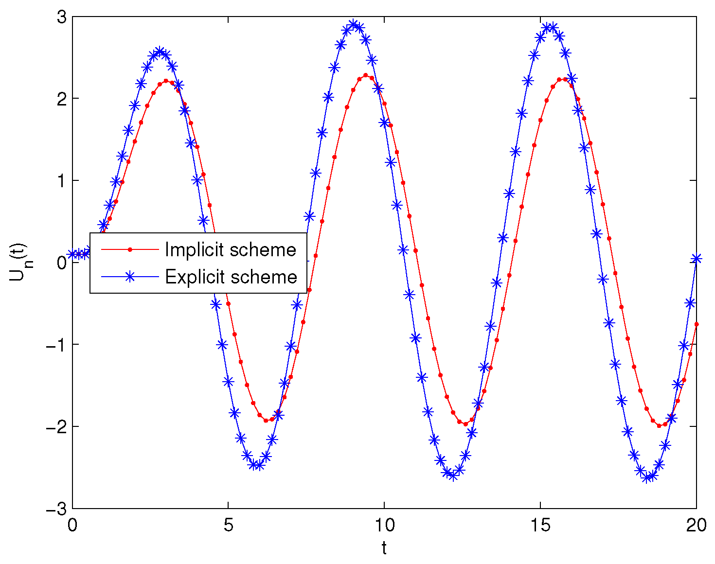
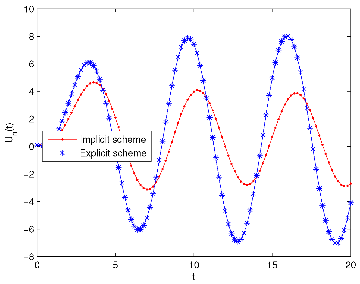
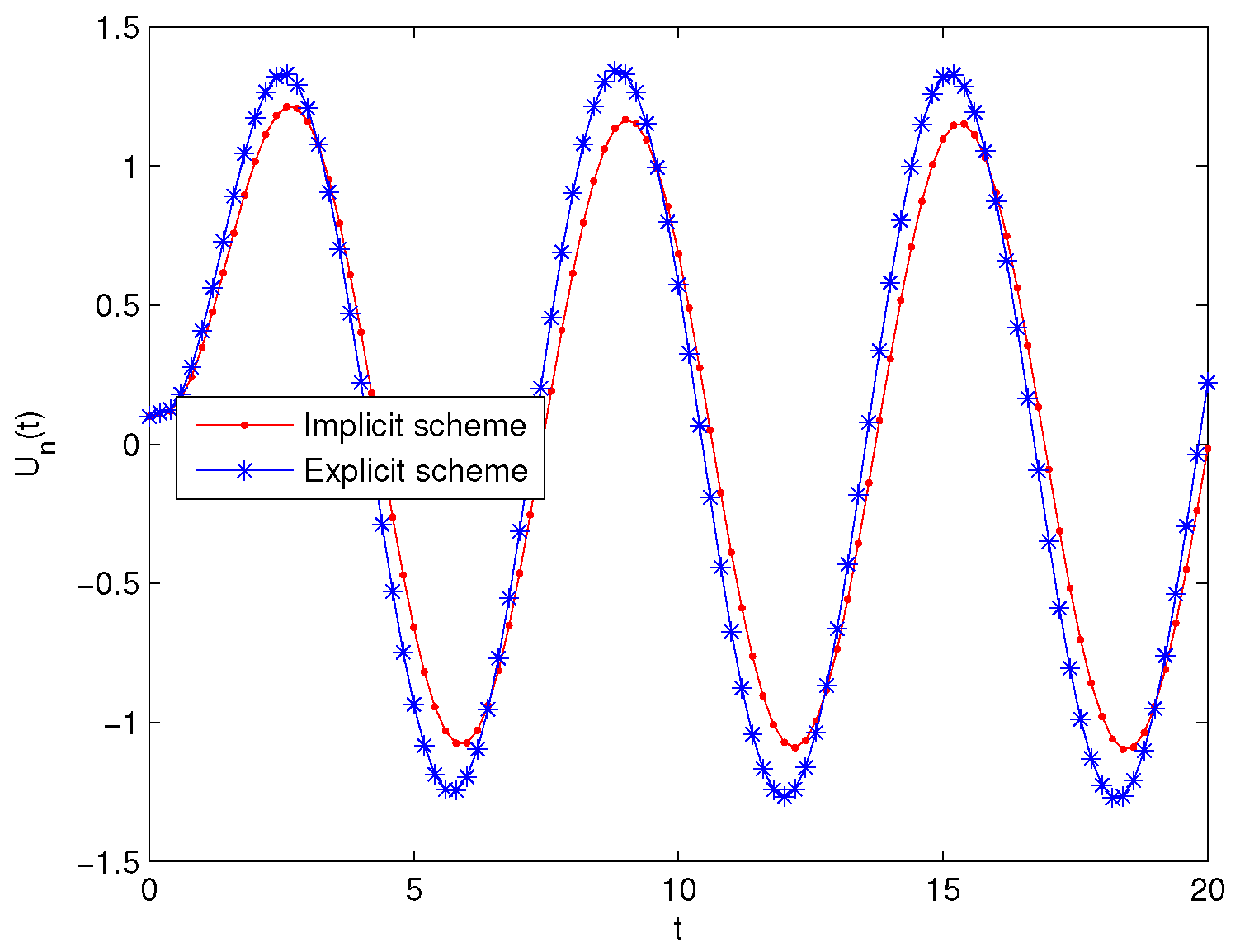
4. Numerical Example

In this section, we provide a numerical example in one-dimensional space to show the validity of our results. We consider the following differential equation

$$\left\{\begin{array}{c}{D}_t^{\alpha }u(t)=-u(t)+J^{1-\alpha }sint,0<t\le 20,\hfill \\ u(0)=0.1,\hfill \end{array}\right.$$

(13)

in Euclidean space $\mathbb{R}$, when ${\tau }_n=0.2$ and $\alpha$ equals $0.5,0.25,0.7$, respectively.

According to Figure 1, Figure 2 and Figure 3, one can see that the solutions of implicit schemes are stable. Therefore, Theorem 4 is valid by means of these Figures. On the other hand, one can see that the solutions of explicit schemes are unstable in Figure 1 and Figure 2. The solution of explicit scheme is shown to be stable in Figure 3. Thus, Theorem 5 is also valid, since $\alpha$ must be greater than $0.5$ in this theorem.

5. Conclusions

In this work, the existence and stability of two difference schemes for nonhomogeneous fractional Cauchy problem are obtained in the space $C(E_n)$ using of the methods of numerical analysis and functional analysis. These approaches are efficient, simple and can be applied to analogous problems. In the near future, we will investigate the order of convergence of difference schemes and stability for problem (3) in suitable spaces.

References

1. Guidetti, D.; Karasözen, B.; Piskarev, S. Approximation of abstract differential equations. J. Math. Sci. 2004, 122, 3013–3054. [Google Scholar] [CrossRef]
2. Li, M.; Morozov, V.; Piskarev, S. On the approximations of derivatives of integrated semigroups. J. Inverse Ill-Posed Probl. 2010, 18, 515–550. [Google Scholar] [CrossRef]
3. Li, M.; Morozov, V.; Piskarev, S. On the approximations of derivatives of integrated semigroups II. J. Inverse Ill-Posed Probl. 2011, 19, 643–688. [Google Scholar] [CrossRef]
4. Abdelaziz, N.H. On approximation by discrete semigroups. J. Approx. Theory 1993, 73, 253–269. [Google Scholar] [CrossRef]
5. Abdelaziz, N.H.; Chernoff, P.R. Continuous and discrete semigroup approximations with applications to the Cauchy problem. J. Oper. Theory 1994, 32, 331–352. [Google Scholar]
6. Ashyralyev, A.; Sobolevskii, P.E. Well-posedness of Parabolic Difference Equations. In Operator Theory; Springer: Basel, Switzerland; Boston, MA, USA; Berlin, Germany; Birkhäuser: Basel, Switzerland, 1994; Volume 69. [Google Scholar]
7. Cao, Q.; Pastor, J.; Siegmund, S.; Piskarev, S. The approximations of parabolic equations at the vicinity of hyperbolic equilibrium point. Numer. Funct. Anal. Optim. 2014, 35, 1287–1307. [Google Scholar] [CrossRef]
8. Piskarev, S. Differential Equations in Banach Space and Their Approximation; Moscow State University Publish House: Moscow, Russia, 2005. (In Russian) [Google Scholar]
9. Vainikko, G. Approximative methods for nonlinear equations (two approaches to the convergence problem). Nonlinear Anal. 1978, 2, 647–687. [Google Scholar] [CrossRef]
10. Alam, M.M.; Dubey, S. Strict Hölder regularity for fractional order abstract degenerate differential equations. Ann. Funct. Anal. 2022, 13, 1–29. [Google Scholar] [CrossRef]
11. Alikhanov, A.A. A new difference scheme for the time fractional diffusion equation. J. Comput. Phys. 2015, 280, 424–438. [Google Scholar] [CrossRef] [Green Version]
12. Bajlekova, E. Fractional Evolution Equations in Banach Spaces. Ph.D. Thesis, University Press Facilities, Eindhoven University of Technology, Eindhoven, The Netherlands, 2001. [Google Scholar]
13. Fan, Z.; Dong, Q.; Li, G. Almost exponential stability and exponential stability of resolvent operator families. Semigroup Forum 2016, 93, 491–500. [Google Scholar] [CrossRef]
14. Fan, Z. A short note on the solvability of impulsive fractional differential equations with Caputo derivatives. Appl. Math. Lett. 2014, 38, 14–19. [Google Scholar] [CrossRef]
15. Gao, G.; Sun, Z. The finite difference approximation for a class of fractional sub-diffusions on a space unbounded domain. J. Comput. Phys. 2013, 236, 443–460. [Google Scholar] [CrossRef]
16. He, J.W.; Zhou, Y. Hölder regularity for non-autonomous fractional evolution equations. Fract. Calc. Appl. Anal. 2022, 25, 378–407. [Google Scholar] [CrossRef]
17. Kilbas, A.A.; Srivastava, H.M.; Trujillo, J.J. Theory and Applications of Fractional Differential Equations. In North-Holland Mathematics Studies; Elsevier: Amsterdam, The Netherlands, 2006; Volume 204. [Google Scholar]
18. Li, K.; Peng, J.; Jia, J. Cauchy problems for fractional differential equations with Riemann-Liouville fractional derivatives. J. Funct. Anal. 2012, 263, 476–510. [Google Scholar] [CrossRef] [Green Version]
19. Liang, Y.; Shi, Y.; Fan, Z. Exact solutions and Hyers-Ulam stability of fractional equations with double delays. Fract. Calc. Appl. Anal. 2023, 26, 439–460. [Google Scholar] [CrossRef]
20. Liu, L.; Fan, Z.; Li, G.; Piskarev, S. Maximal regularity for fractional Cauchy equation in Hölder space and its approximation. Comput. Methods Appl. Math. 2019, 19, 779–796. [Google Scholar] [CrossRef]
21. Liu, L.B.; Liang, Z.; Long, G.; Liang, Y. Convergence analysis of a finite difference scheme for a Riemann-Liouville fractional derivative two-point boundary value problem on an adaptive grid. J. Comput. Appl. Math. 2020, 375, 112809. [Google Scholar] [CrossRef]
22. Liu, R.; Li, M.; Piskarev, S. Stability of difference schemes for fractional equations. Differ. Equ. 2015, 51, 904–924. [Google Scholar] [CrossRef]
23. Liu, R.; Li, M.; Piskarev, S. Approximation of semilinear fractional Cauchy problem. Comput. Methods Appl. Math. 2015, 15, 203–212. [Google Scholar] [CrossRef]
24. Liu, R.; Li, M.; Piskarev, S. The order of convergence of difference schemes for fractional equations. Numer. Funct. Anal. Optim. 2017, 38, 754–769. [Google Scholar] [CrossRef]
25. Liu, R.; Li, M.; Pastor, J.; Piskarev, S. On the approximation of fractional resolution families. Differ. Equ. 2014, 50, 927–937. [Google Scholar] [CrossRef]
26. Podlubny, I. Fractional Differential Equations; Academic Press: San Diego, CA, USA, 1999. [Google Scholar]
27. Ponce, R. Time discretization of fractional subdiffusion equations via fractional resolvent operators. Comput. Math. Appl. 2020, 80, 69–92. [Google Scholar] [CrossRef]
28. Ponce, R. Well-posedness of second order differential equations with memory. Math. Nachr. 2022, 295, 2246–2264. [Google Scholar] [CrossRef]
29. Prüss, J. Evolutionary Integral Equations and Applications; Birkhäuser: Basel, Switzerland; Berlin, Germany, 1993. [Google Scholar]
30. Shi, Y.; Fan, Z.; Li, G. New explicit solutions and Hyers-Ulam stability of fractional delay differential equations. J. Yangzhou Univ. (Nat. Sci. Ed.) 2023, 26, 1–5+19. (In Chinese) [Google Scholar]
31. Wang, R.N.; Chen, D.H.; Xiao, T.J. Abstract fractional Cauchy problems with almost sectorial operators. J. Diff. Equ. 2012, 252, 202–235. [Google Scholar] [CrossRef] [Green Version]
32. Zhang, J.; Wang, J.R.; Zhou, Y. Numerical analysis for time-fractional Schrödinger equation on two space dimensions. Adv. Differ. Equ. 2020, 2020, 53. [Google Scholar] [CrossRef]
33. Zhu, S.; Fan, Z.; Li, G. Topological characteristics of solution sets for fractional evolution equations and applications to control systems. Topol. Methods Nonlinear Anal. 2019, 54, 177–202. [Google Scholar] [CrossRef]
Figure 1. α = 0.5 .
Symmetry 15 01355 g001
Figure 2. α = 0.25 .
Symmetry 15 01355 g002
Figure 3. α = 0.75 .
Symmetry 15 01355 g003
Disclaimer/Publisher’s Note: The statements, opinions and data contained in all publications are solely those of the individual author(s) and contributor(s) and not of MDPI and/or the editor(s). MDPI and/or the editor(s) disclaim responsibility for any injury to people or property resulting from any ideas, methods, instructions or products referred to in the content.