A New Right-Skewed One-Parameter Distribution with Mathematical Characterizations, Distributional Validation, and Actuarial Risk Analysis, with Applications

Abstract

Skewed probability distributions are important when modeling skewed data sets because they provide a way to describe the shape of the distribution and estimate the likelihood of extreme events. Asymmetric probability distributions have the potential to handle and assess problems in actuarial risk assessment and analysis. To that end, we present a new right-skewed one-parameter distribution. In this work and for this purpose, a right-skewed probability distribution was derived and analyzed. The new distribution outperformed the exponential distribution, the Pareto distribution, the Chen distribution, and others in the field of actuarial risk analysis. Some useful key risk indicators are considered and analyzed to analyze the risks and for comparison with the competitive model. Several actuarial risk functions and indicators are evaluated and analyzed using the U.K. insurance claims data set. The process of risk assessment and analysis was carried out using a comprehensive simulation. For the purposes of distributional validity, a modified chi-squared type test is presented and employed in the testing process. The new, modified chi-squared type test that is used is simply an extension of the Rao–Robson–Nikulin test. In this work, the distributional validity is presented and analyzed under right-skewed censored and uncensored data sets.

1. Introduction

Skewed distributions are important in insurance and the actuarial sciences because they help insurers and actuaries to understand the frequency and severity of potential losses. In the insurance industry, loss data are often modeled using a skewed distribution such as the lognormal distribution, which is commonly used to model losses in areas such as natural disasters, medical malpractice, and product liability. By using a skewed distribution, insurers can better estimate the likelihood and potential magnitude of losses, which is important for pricing policies and when managing risk. For this main purpose, we present a new asymmetric distribution, called the right-skewed exponential (RSEx) distribution, which has high flexibility in terms of its probability density function (PDF) and its failure rate function (FRF). The RSEx distribution is recommended as an adequate alternative to the well-known exponential (Ex) distribution.

However, the traditional Ex distribution is a probability distribution that models the time between events in a Poisson process, where the events occur continuously and independently at a constant average rate. It is often used in actuarial risk analysis and insurance due to its simplicity and applicability to various scenarios. It has the crucial characteristic of being memoryless and it can be considered as the continuous version of the geometric distribution theory proposed by Kemp [1]. One of the most important characteristics of exponential distribution is its memoryless property. This means that the distribution of time to the next event does not depend on how much time has already passed. This property makes it suitable for modeling scenarios where past history does not affect the future occurrence of events. The Ex distribution is employed in several different applications, in addition to the study of Poisson point processes. The Ex distribution is the only continuous probability distribution with a constant FRF.

The RSEx distribution is very similar to the exponential distribution in regard to some properties and it has only one parameter. However, the mathematical form of the RSEx distribution differs from the exponential distribution. Thus, statistical properties such as moments, function-generating moments, etc., will be different and may need more effort to derive them. In addition, the parameter range of the new distribution differs from the parameter range of the exponential distribution. The parameter of the new distribution is $\theta$, the range of which depends on and is related to the random variable (RV). In this paper, we do not pay much attention to the theoretical results or to the properties of mathematics and algebraic derivations. This is because the main objective of the paper is to explore and illustrate the importance of the new distribution in practice and its significance in the areas of statistical modeling, as well as in the field of application to actuarial risks. However, it may be easy to study any probability distribution theoretically, but it is not at all easy to prove the importance of the new distribution from the practical perspective and from the point of view of statistical modeling. By studying the statistical literature, we will find many distributions that are a generalization of the exponential distribution. Most of these extensions have a large number of parameters (often more than two). However, the RSEx distribution contains only one parameter; this is the first advantage of the new distribution, even before it has been studied. The survival function (SF) of the RSEx model can be expressed as:

$$S_{\theta }\left(\mathcal{x}\right)=\mathit{log}\left(\mathcal{x}-\theta +e\right)e\mathcal{x}p\left[-\left(e^{\mathcal{x}-\theta }-1\right)\right]{|}_{\mathcal{x}\ge \theta },$$

(1)

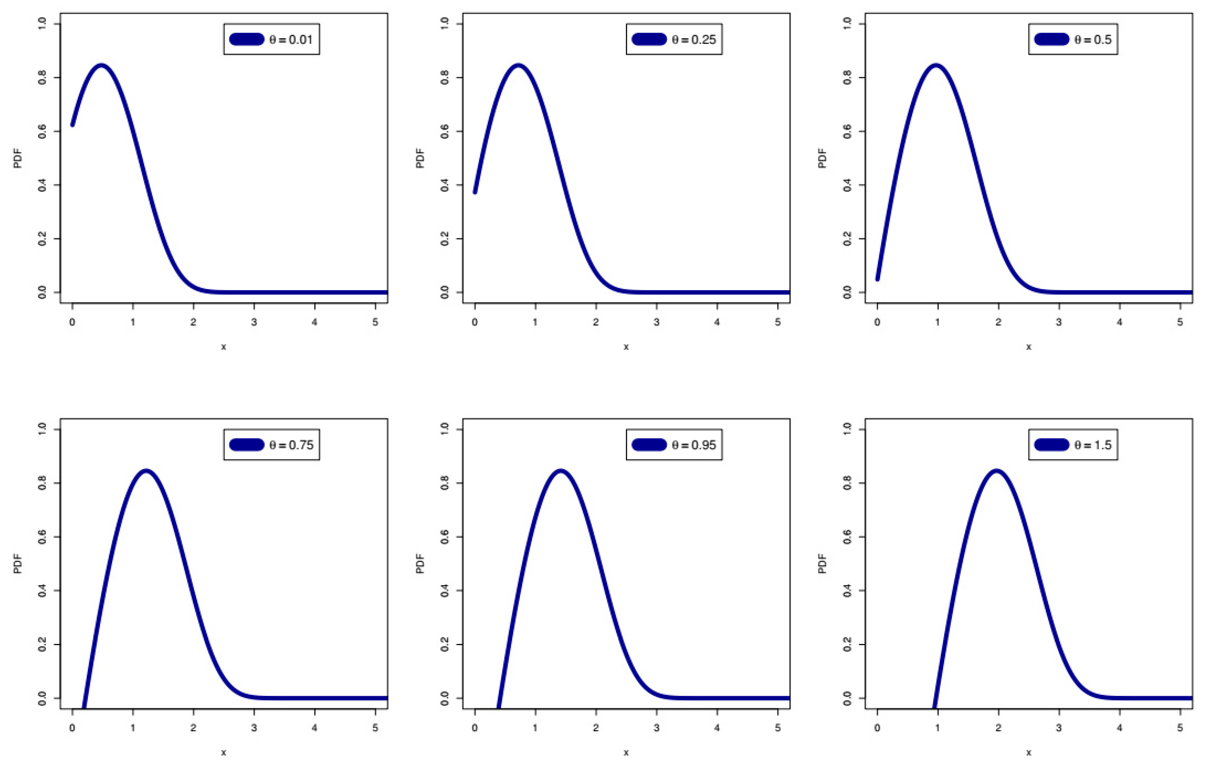
where $e$ is the base for the natural log. The corresponding PDF of the RSEx can be written as:

$$f_{\theta }\left(\mathcal{x}\right)=e\mathcal{x}p\left[-\left(e^{\mathcal{x}-\theta }-1\right)\right]\left[\mathit{log}\left(\mathcal{x}-\theta +e\right)e^{\mathcal{x}-\theta }-\frac{1}{\mathcal{x}-\theta +e}\right]{|}_{\mathcal{x}>\theta }.$$

(2)

The cumulative distribution function (CDF) corresponding to (1) can be expressed as $F_{\theta }\left(\mathcal{x}\right)=1-S_{\theta }\left(\mathcal{x}\right).$ While the Ex distribution achieves the relationship Pr $(\mathcal{T}>\mathcal{s}+t|\mathcal{T}>\mathcal{s})=$ Pr $(\mathcal{T}>t)=e^{\theta t}$ $\forall$ $t\ge 0$, the memoryless capacity does not exist with the RSEx model, where Pr $(\mathcal{T}>\mathcal{s}+t|\mathcal{T}>\mathcal{s})={\mathit{log}}_{\left(\mathcal{s}-\theta +e\right)}\left(\mathcal{s}+t-\theta +e\right)e\mathcal{x}p\left(e^{\mathcal{s}-\theta }-e^{\mathcal{s}+t-\theta }\right)\ne$ Pr $(\mathcal{T}>t)$.

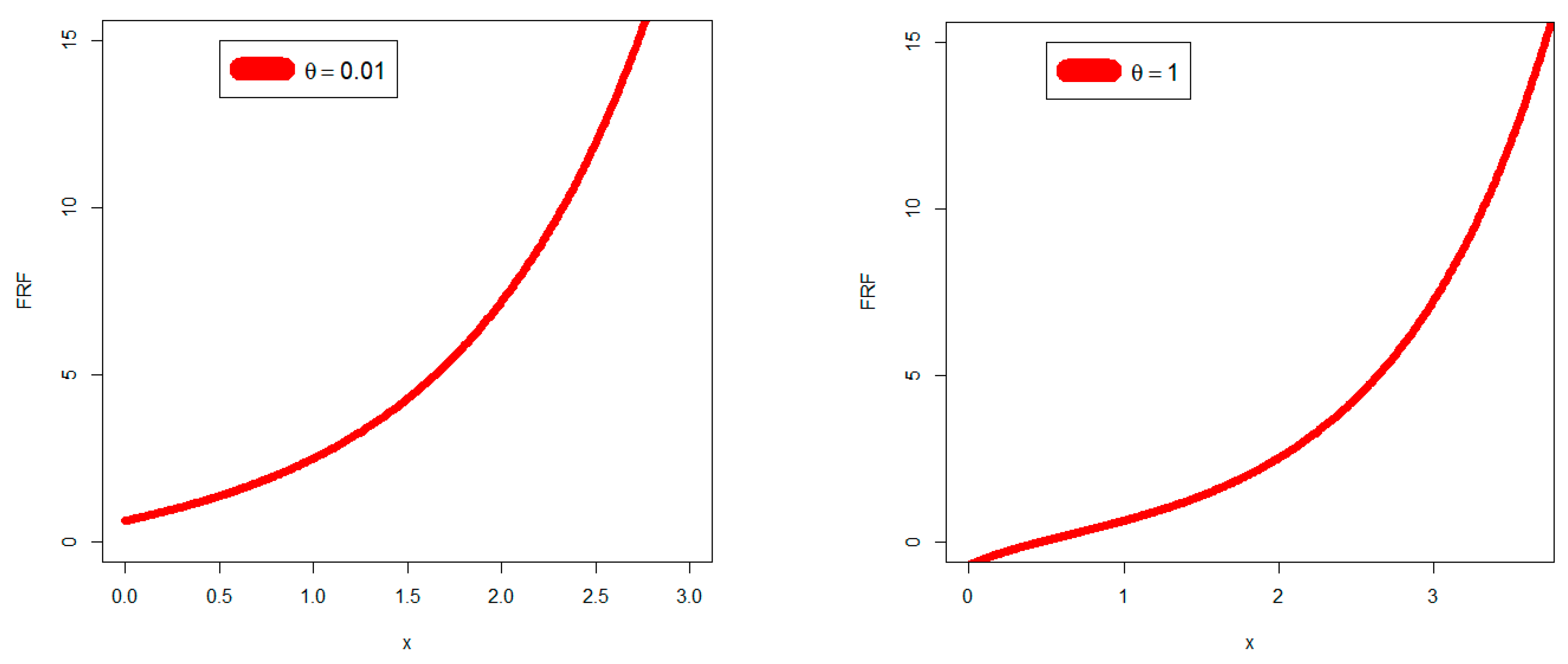
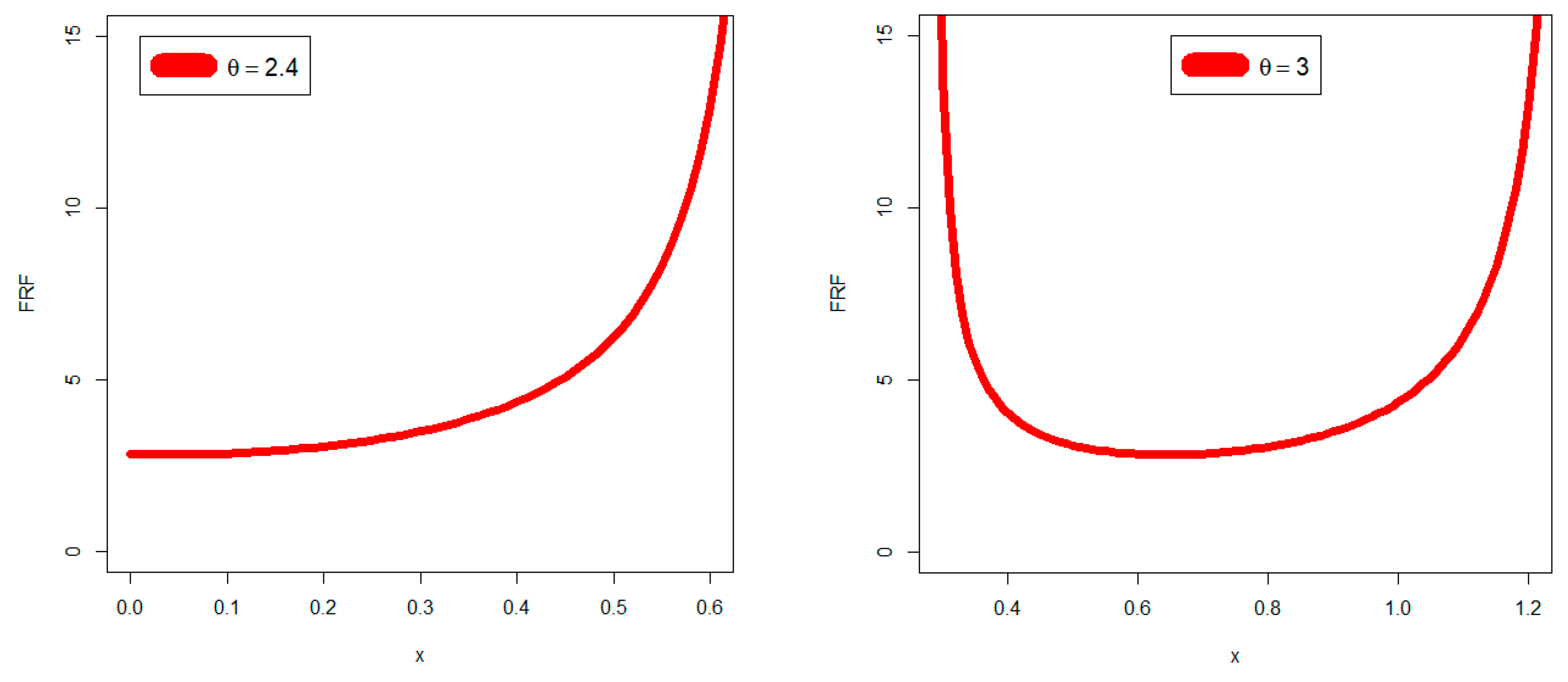
A special section is devoted to the characterization of the RSEx distribution: (i) based on two truncated moments and (ii) in terms of the FRF. For characterization (i), the CDF does not need to have a closed form. Characterizations (i) and (ii) will be presented in Section 2. The FRF, which is sometimes referred to as the danger rate, solely relates to broken objects. It is essential when creating secure software applications and the engineering, financial, insurance, and regulatory sectors frequently rely on it. The FRF represents the frequency with which an engineered system or component fails, expressed in terms of failures per unit of time, and is often used in reliability engineering. The failure rate of a system usually depends on time. The FRF of the RSEx can be expressed as:

$$h_{\theta }\left(\mathcal{x}\right)=e^{\mathcal{x}-\theta }-{\left[\mathit{log}\left(\mathcal{x}-\theta +e\right)\left(\mathcal{x}-\theta +e\right)\right]}^{-1}.$$

(3)

Recently, actuaries have analyzed some actual insurance data using several new continuous distributions (see, for example, Hamed et al. [2], Shrahili et al. [3], and Mohamed et al. [4,5,6]. The skewness of the insurance data sets can be left, right, or right with heavy tails. In this study, we describe how a skewed U.K. insurance claims data set may be described using the flexible continuous asymmetric heavy-tailed RSEx distribution. Despite its enormous potential, using U.K. skewed insurance claims data is tricky. Moreover, identifying its quality and calculating the number of incomplete or missing observations represent the biggest challenge (see Stein et al. [7], Hogg and Klugman [8], Lane [9], and Ibragimov and Prokhorov [10] for more details).

To model insurance payment data, and more specifically, to model huge insurance claim payment data, many research studies have used the Pareto and lognormal distributions. Several academics have employed a modified Pareto distribution (see Beirlant et al. [11]).

Usually, only one number is used to describe the level of risk exposure. These risk exposure levels, sometimes known as key risk indicators (KRIs), are unmistakably the actuarial functions of a certain model that are used in insurance, actuarial science, and financial risk analysis for portfolios and securities. Actuaries and risk managers can learn from such KRIs to identify how exposed a company is to various dangers. Value-at-risk (VAR), conditional-value-at-risk (CVAR), tail variance (TV), tail-value-at-risk (TVAR), and tail mean-variance (TMV) are just a few of the KRIs that can be taken into account. In particular, the VAR is a quantile of the distribution of total losses. Actuaries and risk managers typically focus on using the VAR indicator to show the probability of a poor result at a specific probability/confidence level (see Artzner [12] and Figueiredo et al. [13] for more details).

The process of assessing the actuarial risks or other risks, of course, requires validation testing from another aspect of the analysis. This validation testing can be performed through the well-known goodness-of-fit tests or by presenting a new or at least modified goodness-of-fit test. In this work, the Barzilai–Borwein (BB) algorithm is used for this purpose. The construction of the Rao–Robson–Nikulin (RRNU) statistic for the RSEx model under uncensored case conditions is presented in detail; a simulation study for assessing the RRNU statistics under uncensored case conditions is performed. Four real-world data application scenarios are presented under uncensored case conditions: the first uncensored data set comprises reliability data on carbon fibers, the second uncensored data set is of the heat exchanger tube crack data, the third uncensored data set concerns the various strengths of glass fibers, and the fourth uncensored data set comprises gene-based breast cancer data. Moreover, the construction of the RRNU statistic for the RSEx model under censored case conditions is presented in detail, and a simulation study for assessing the RRNU statistics under censored case conditions is presented. Four censored real-world data applications are analyzed under censored case conditions: the first one comprises data on cancer of the lung, the second data set concerns capacitor reliability data, the third data set is on aluminum cells under reduction conditions, and the fourth data set comprises head and neck cancer data. In this paper, the RSEx distribution is examined from a different angle. Using four different applications and a broad collection of simulation experiences, we dealt with the numerous theoretical and applied aspects. We have not overlooked the theory of statistical hypothesis testing and distributional verification in this context; to prove it, we provided eight examples through study and analysis, four of which used complete data sets and four of which used censored data sets. Moreover, two different ways to characterize the RSEx distribution are discussed herein, such as characterization using two truncated moments and characterization using the FRF. The innovations of this study can be highlighted as follows:

• We present a new right-skewed one-parameter distribution, which can be considered as an alternative to the Chen distribution, Pareto type II (PaII) distribution, and generalized gamma (GG) distribution.
• We analyze an actuarial data set with the new model as well as with some competing models, such as the Chen distribution, PaII distribution, and GG distribution due to certain risk indicators.
• We present a new type test for uncensored data sets, with four applications for uncensored distributional validation.
• We present a new, modified type test for censored data sets, with examples of censored distributional validation.
• The new model is characterized by a probability density function that is more flexible than the probability density functions of its competing distributions; the research indicated that it can be nominated as an alternative distribution.
• The new failure rate function includes many forms suitable for modeling real-world data in various engineering, medical, and other fields, and nine examples have been presented to support this finding.

2. Graphical Presentation and Some Mathematical Properties

2.1. Graphical Presentation

In probability theory, the concept of symmetry refers to the shape of a probability distribution. A symmetric probability distribution is one in which the left and right sides of the distribution are mirror images of each other. In other words, if a vertical line is drawn at the center of the distribution, the left and right sides of the distribution will be identical. The most well-known example of a symmetric distribution is normal distribution, which is often used in statistics to model many real-world phenomena. A normal distribution has a bell-shaped curve, with the mean and median located at the center of the curve. Because the normal distribution is symmetric, the mean, median, and mode are all the same. However, not all probability distributions are symmetric. Some distributions are asymmetric, meaning that they do not have mirror-image left and right sides. Asymmetric distributions are often referred to as skewed distributions. Skewed distributions also have important applications in probability theory, as discussed in previous papers. In this subsection, we present a graphical study of the new RSEx distribution from two different perspectives. The first is a graphical study of the new density function, to explore the flexibility of the new distribution. The second is a graphical study of the new failure rate function, to explore the flexibility and importance of the new distribution. It should be noted that the importance of the new distributions depends on several factors, including these two factors. Figure 1 shows some possible PDF plots of RSEx distributions for selected parameter values, while Figure 2 shows some possible FRF plots of RSEx distributions for selected parameter values.

Based on Figure 1, it can be seen that the RSEx distribution has an asymmetric heavy tail on the right and that the distribution always has one peak. Based on Figure 2, it is clear that the FRF of the RSEx distribution shows important shapes and demonstrates new patterns that are not found in the Ex distribution, including the monotonically increasing FRF, J-FRF (constant–increasing FRF), and bathtub-FRF (decreasing–constant–increasing FRF). The diversity in the forms included in the densities and the corresponding failure rates represent one of the most important aspects that show the importance of the new distribution and its high level of flexibility.

2.2. Mathematical Properties

2.2.1. Asymptotics for CDF, PDF, and FRF

The importance of asymptotic properties lies in the fact that they allow us to make statistical inferences using large sample sizes. Asymptotic results provide valuable information about the behavior of a statistical estimator or test statistic as the sample size increases, and this information can then be used to derive important statistical properties and make inferences regarding the population. The asymptotics of CDF, PDF, and FRF for RSEx($\theta$) as $\mathcal{x}\to {\theta }^{+}$ are given by:

$$F\left(\mathcal{x}\right)\sim \mathcal{x}-\theta ,f\left(\mathcal{x}\right)\sim 1,h\left(\mathcal{x}\right)\sim \frac{1}{1-\mathcal{x}+\theta }.$$

The asymptotics of CDF, PDF, and FRF for RSEx($\theta$) as $\mathcal{x}\to +\infty$ are given by:

$$1-F\left(\mathcal{x}\right)\sim e^{-e^{\mathcal{x}}}\mathit{log}(\mathcal{x}),f\left(\mathcal{x}\right)\sim e^{-e^{\mathcal{x}}}\mathit{log}(\mathcal{x}),h\left(\mathcal{x}\right)\sim 1.$$

Asymptotic theory is used to approximate the distribution of statistical estimators and test statistics when the sample size grows very large. This allows for an approximation of the exact distribution of the statistic, which may otherwise be difficult to derive.

2.2.2. Moments

Let $X\sim \mathrm{RSEx}\left(\theta \right)$; then, the CDF of $Y=X-\theta$ is given by:

$$F_Y\left(\mathcal{y}\right)=1-\mathit{log}(\mathcal{y}+e)e^{-\left(e^{\mathcal{y}}-1\right)},\hspace{0.33em}\hspace{0.33em}\mathcal{y}>0.$$

The nth moment of $Y$ is given by:

$$\begin{array}{l}E\left(Y^n\right)=n{{\displaystyle \int }}_0^{+\infty }{\mathcal{y}}^{n-1}\left[1-F_Y\left(\mathcal{y}\right)\right]d\mathcal{y}=n{{\displaystyle \int }}_0^{+\infty }{\mathcal{y}}^{n-1}\mathit{log}(\mathcal{y}+e)e^{-\left(e^{\mathcal{y}}-1\right)}d\mathcal{y}\\ \hspace{1em}\hspace{1em}\hspace{1em}\hspace{1em}\hspace{1em}\hspace{1em}\hspace{1em}=ne\left[I_1^{0,e}\left(\mathcal{y}\right)+I_2^{e,+\infty }\left(\mathcal{y}\right)\right],\end{array}$$

where:

$$I_1^{0,e}\left(\mathcal{y}\right)={{\displaystyle \int }}_0^e{\mathcal{y}}^{n-1}\mathit{log}(\mathcal{y}+e)e^{-\left(e^{\mathcal{y}}-1\right)}d\mathcal{y},$$

and:

$$I_2^{e,+\infty }\left(\mathcal{y}\right)={{\displaystyle \int }}_e^{+\infty }{\mathcal{y}}^{n-1}\mathit{log}(\mathcal{y}+e)e^{-\left(e^{\mathcal{y}}-1\right)}d\mathcal{y}.$$

Now, we compute $I_1^{0,e}\left(\mathcal{y}\right)$ and $I_2^{e,+\infty }\left(\mathcal{y}\right)$. Note that for $0<\mathcal{y}<e$,

$$\mathit{log}(\mathcal{y}+e)=\mathit{log}\left[e\left(1+\frac{\mathcal{y}}{e}\right)\right]=1+\mathit{log}\left(1+\frac{\mathcal{y}}{e}\right)=1+{\displaystyle \sum }_{\mathcal{w}=0}^{+\infty }{\left(\frac{\mathcal{y}}{e}\right)}^{\mathcal{w}+1}\frac{1}{\mathcal{w}+1}={\displaystyle \sum }_{\mathcal{w}=0}^{+\infty }{\mathcal{a}}_{\mathcal{w}}{\mathcal{y}}^{\mathcal{w}},$$

where ${\mathcal{a}}_0=1$ and ${\mathcal{a}}_{\mathcal{w}}=\frac{1}{\mathcal{w}{e}^{\mathcal{w}}}$ for $\mathcal{w}\ge 1$. Then:

$$I_1^{0,e}\left(\mathcal{y}\right)={\displaystyle \sum }_{\mathcal{w}=0}^{+\infty }{\mathcal{a}}_{\mathcal{w}}{{\displaystyle \int }}_0^e{\mathcal{y}}^{n+\mathcal{w}-1}{e}^{-e^{\mathcal{y}}}d\mathcal{y}.$$

By changing $u=e^{\mathcal{y}}$, we obtain:

$$I_2^{e,+\infty }\left(\mathcal{y}\right)={\displaystyle \sum }_{\mathcal{w}=0}^{+\infty }{\mathcal{a}}_{\mathcal{w}}{{\displaystyle \int }}_1^{e^e}\left[\mathit{log}(u\right){]}^{n+\mathcal{w}-1}\hspace{0.33em}\frac{e^{-u}}{u}du.$$

The last integral can be obtained numerically:

$$I_2^{e,+\infty }\left(\mathcal{y}\right)={{\displaystyle \int }}_e^{+\infty }{\mathcal{y}}^{n-1}\mathit{log}(\mathcal{y}+e)e^{-e^{\mathcal{y}}}d\mathcal{y}.$$

Note that for $\mathcal{y}>e$,

$$\mathit{log}(\mathcal{y}+e)=\mathit{log}\left[\mathcal{y}\left(1+\frac{e}{\mathcal{y}}\right)\right]=\mathit{log}(\mathcal{y})+\mathit{log}\left(1+\frac{e}{\mathcal{y}}\right)=\mathit{log}(\mathcal{y})+{\displaystyle \sum }_{\mathcal{w}=0}^{+\infty }{\left(\frac{e}{\mathcal{y}}\right)}^{\mathcal{w}+1}\frac{1}{\mathcal{w}+1}.$$

Then:

$$I_2^{e,+\infty }\left(\mathcal{y}\right)={{\displaystyle \int }}_e^{+\infty }{\mathcal{y}}^{n-1}\left[\mathit{log}(\mathcal{y})+{\displaystyle \sum }_{\mathcal{w}=0}^{+\infty }{\left(\frac{e}{\mathcal{y}}\right)}^{\mathcal{w}+1}\frac{1}{\mathcal{w}+1}\right]e^{-e^{\mathcal{y}}}d\mathcal{y},$$

which implies:

$$I_2^{e,+\infty }\left(\mathcal{y}\right)={{\displaystyle \int }}_e^{+\infty }{\mathcal{y}}^{n-1}\mathit{log}(\mathcal{y})e^{-e^{\mathcal{y}}}d\mathcal{y}+{\displaystyle \sum }_{\mathcal{w}=0}^{+\infty }\frac{e^{\mathcal{w}+1}}{\mathcal{w}+1}{{\displaystyle \int }}_e^{+\infty }\frac{e^{-e^{\mathcal{y}}}}{{\mathcal{y}}^{\mathcal{w}+2-n}}.$$

The last integrals can be obtained numerically. Finally,

$$E\left(X^n\right)=E\left(Y-\theta \right)={\displaystyle \sum }_{k=0}^n\left(\begin{array}{c}n\\ k\end{array}\right){\left(-\theta \right)}^{k}E\left(Y^{n-K}\right).$$

3. Characterization Results

3.1. Characterizations Based on Two Truncated Moments

The mathematical characterization, which is based on two truncated moments, provides valuable insights into the behavior and distribution of RVs within specific ranges. It offers robustness, facilitates parameter estimation, enables distributional modeling, aids in risk assessment, supports hypothesis testing, and assists in model selection and goodness-of-fit evaluations. These mathematical properties make truncated moments a powerful tool for analyzing and interpreting data that are subject to truncation or fall within a restricted interval. In this subsection, we characterize the RSEx distribution based on a simple relationship between two truncated moments. The first characterization applies a theorem developed by Glanzel [14], Theorem 1, which is given below. Clearly, the result holds just as well when the $H_{\left[d,e\right]}$ is not a closed interval. This characterization is stable in the sense of weak convergence (see Glanzel [15]).

Theorem 1.

Let $\left(\mathsf{\omega },F,P\right)$ be a given probability space and let $H_{\left[d,e\right]}=\left[d,e\right]$ be an interval for some $d<e$ $\left(d=-+\infty , when e=+\infty \mathit{might} \mathit{also} \mathit{be} \mathit{allowed}\right).$

Let $X\hspace{0.33em}\hspace{0.33em}:\mathsf{\omega }\to H_{\left[d,e\right]}$ be a continuous random variable (CRV), with the distribution function $F,$ and let $\mathcal{Q}$ and $h$ be two real functions defined on $H_{\left[d,e\right]},$ such that:

$$E\left[{\mathcal{Q}}_{\theta }\left(X\right) | X\ge \mathcal{x}\right]=E\left[h_{\theta }\left(X\right) | X\ge \mathcal{x}\right]{\mathcal{G}}_{\theta }\left(\mathcal{x}\right){|}_{\mathcal{x}\in H_{\left[d,e\right]}},$$

is defined with a real function, $\mathcal{G}$. Assume that $\mathcal{Q}\left(\cdot \right)$, $h\left(\cdot \right)\in {\mathcal{C}}^1\left(H_{\left[d,e\right]}\right)$, $\mathcal{G}\in {\mathcal{C}}^2\left(H_{\left[d,e\right]}\right),$ and $F$ is twice the continuously differentiable and strictly monotone function on the set $H_{\left[d,e\right]}$. Finally, assume that the equation $\mathcal{G}h=\mathcal{Q}$ has no real solution in the interior of $H_{\left[d,e\right]}$. Then, $F$ is uniquely determined by the functions $\mathcal{Q}\left(\cdot \right)$, $h\left(\cdot \right)$ and $\mathcal{G}\left(\cdot \right)$, particularly:

$$F\left(\mathcal{x}\right)={{\displaystyle \int }}_{\mathcal{a}}^{\mathcal{x}}\mathcal{C}\left|\frac{{\mathcal{G}}^{\prime }\left(u\right)}{\mathcal{G}\left(u\right)h\left(u\right)-\mathcal{Q}\left(u\right)}\right|e\mathcal{x}p\left(-\mathcal{s}\left(u\right)\right) du,$$

where the function $\mathcal{s}$ is a solution of the differential equation ${\mathcal{s}}^{\prime }=\frac{{\mathcal{G}}^{\prime } h}{\mathcal{G} h-\mathcal{Q}}$ and $\mathcal{C}$ is the normalization constant, such that ${\int }_{H_{\left[d,e\right]}}dF=1$.

Proposition 1.

Suppose the RV $X\hspace{0.33em}\hspace{0.33em}:\mathsf{\omega }\to \left(\theta ,+\infty \right)$ is continuous, and assume:

$$h_{\theta }\left(\mathcal{x}\right)={\left\{\mathit{log}\left(\mathcal{x}-\theta +e\right)-{\left(\mathcal{x}-\theta +e\right)}^{-1}{e}^{-\left(\mathcal{x}-\theta \right)}\right\}}^{-1},$$

and:

$${\mathcal{Q}}_{\theta }\left(\mathcal{x}\right)=h_{\theta }\left(\mathcal{x}\right)e\mathcal{x}p\left\{1-e^{\left(\mathcal{x}-\theta \right)}\right\}$$

for $x>\theta .$ Then, the density of $X$ is given in (2) if and only if ${\mathcal{G}}_{\theta }\left(\mathcal{x}\right)$ is defined in Theorem 1 as:

$${\mathcal{G}}_{\theta }\left(\mathcal{x}\right)=\frac{1}{2}e\mathcal{x}p\left\{1-e^{\left(\mathcal{x}-\theta \right)}\right\}{|}_{\mathcal{x}>\theta }.$$

Proof. 

If $X$ has the new PDF in (2), then:

$$\left(1-F\left(\mathcal{x}\right)\right)E\left[h_{\theta }\left(X\right) | X\ge \mathcal{x}\right]=e\mathcal{x}p\left\{-\left[e^{\left(\mathcal{x}-\theta \right)}-1\right]\right\}{|}_{\mathcal{x}>\theta },$$

and:

$$\left(1-F\left(\mathcal{x}\right)\right)E\left[{\mathcal{Q}}_{\theta }\left(X\right) | X\ge \mathcal{x}\right]=\frac{1}{2}e\mathcal{x}p\left\{-2\left[e^{\left(\mathcal{x}-\theta \right)}-1\right]\right\}{|}_{\mathcal{x}>\theta },$$

and finally:

$${\mathcal{G}}_{\theta }\left(\mathcal{x}\right)h_{\theta }\left(\mathcal{x}\right)-{\mathcal{Q}}_{\theta }\left(\mathcal{x}\right)=-\frac{1}{2}{h}_{\theta }\left(\mathcal{x}\right)e\mathcal{x}p\left\{-\left[e^{\left(\mathcal{x}-\theta \right)}-1\right]\right\}<0{|}_{\mathcal{x}>\theta }.$$

Conversely, if $\mathcal{G}$ takes the above form, then:

$${\mathcal{s}}^{\prime }\left(\mathcal{x}\right)=\frac{{\mathcal{G}}_{\theta }^{\prime }\left(\mathcal{x}\right)h_{\theta }\left(\mathcal{x}\right)}{{\mathcal{G}}_{\theta }\left(\mathcal{x}\right)h_{\theta }\left(\mathcal{x}\right)-{\mathcal{Q}}_{\theta }\left(\mathcal{x}\right)}=e^{\left(\mathcal{x}-\theta \right)},$$

and hence:

$$\mathcal{s}\left(\mathcal{x}\right)=e^{\left(\mathcal{x}-\theta \right)},\mathcal{x}>\theta .$$

In view of Theorem 1, $X$ has PDF (2). □

Corollary 1.

If $X\hspace{0.33em}:\mathsf{\omega }\to \left(\theta ,+\infty \right)$ is a CRV and $h_{\theta }\left(\mathcal{x}\right)$ is as in Proposition 1, therefore, $X$ has the new PDF in (2) if, and only if, there exist two functions, $\mathcal{Q}\left(\cdot \right)$ and $\mathcal{G}\left(\cdot \right)$, as defined in Theorem 1, and satisfying the following first-order differential equation:

$$\frac{1}{h_{\theta }\left(\mathcal{x}\right){\mathcal{G}}_{\theta }\left(\mathcal{x}\right)-{\mathcal{Q}}_{\theta }\left(\mathcal{x}\right)}{\mathcal{G}}_{\theta }^{\prime }\left(\mathcal{x}\right)h_{\theta }\left(\mathcal{x}\right)=e^{\mathcal{x}-\theta }.$$

Corollary 2.

The general solution of the above differential equation is:

$${\mathcal{G}}_{\theta }\left(\mathcal{x}\right)=e\mathcal{x}p\left\{\left[e^{\left(\mathcal{x}-\theta \right)}-1\right]\right\}\left[-\int e^{\left(\mathcal{x}-\theta \right)}e\mathcal{x}p\left\{-\left[e^{\left(\mathcal{x}-\theta \right)}-1\right]\right\}\frac{{\mathcal{Q}}_{\theta }\left(\mathcal{x}\right)}{h_{\theta }\left(\mathcal{x}\right)}+D\right],$$

where $D$ is a constant.

3.2. Characterization Results Based on FRF

The FRF is a mathematically important characterization found in survival analysis, providing a comprehensive understanding of the risks of events over time. Its mathematical properties and interpretations facilitate the analysis, modeling, and prediction of time-to-event data in various fields, including medical research, engineering, economics, and social sciences. The FRF, $h_F$, of a twice-differentiable distribution function, $F,$ with density $f$, satisfies the following trivial first differential equation:

$$\frac{f{ }^{\prime }\left(\mathcal{x}\right)}{f \left(\mathcal{x}\right)}=\frac{h_F^{\prime }\left(\mathcal{x}\right)}{h_F\left(\mathcal{x}\right)}-h_F\left(\mathcal{x}\right).$$

As we mentioned in our previous works, for many univariate continuous distributions, this is the only characterization based on FRF. Proposition 2, presented below, provides a non-trivial characterization of RSEx distribution.

Proposition 2.

Suppose $X\hspace{0.33em}:\mathsf{\omega }\to \left(\theta ,+\infty \right)$ is a CRV. The density of $\hspace{0.33em}X$ is (2) if, and only if, the differential equation holds:

$$h_F^{\prime }\left(\mathcal{x}\right)-h_F\left(\mathcal{x}\right)=\frac{\left(\mathcal{x}-\theta +e+1\right)\mathit{log}\left(\mathcal{x}-\theta +e\right)+1}{{\left[\left(\mathcal{x}-\theta +e\right)\mathit{log}\left(\mathcal{x}-\theta +e\right)\right]}^2}, \mathcal{x}>\theta ,$$

with the initial condition, $h_F\left(\theta \right)=\frac{e-1}{e}$.

Proof. 

This is straightforward and, hence, is omitted. □

4. The KRIs

4.1. The VAR

The VARq indicator is a widely used measure in financial risk management and has numerous applications in actuarial risk analysis and insurance. The VARq provides an estimate of the potential loss that an institution or portfolio may experience within a given confidence level over a specific time horizon. In actuarial risk analysis, VARq is used to assess the potential downside risk of insurance portfolios. It helps actuaries and risk managers to quantify the likelihood and severity of losses that could be incurred by an insurance company, due to various factors such as natural disasters, accidents, or other unforeseen events. The VaR of the loss RV $X$ at the 100q% level, say, VARq($X$) or $\mathsf{\pi }\left(q\right)$, is the 100q% quantile (or percentile) of the distribution of $X$. Then, we have:

$$\mathrm{Pr}\left\{X>Q_u|Q_u=F_{\theta }^{-1}\left(\mathcal{x}\right)\right\}=\left\{\begin{array}{l}1\%{|}_{q=99\%}\hspace{1em}\\ 5\%{|}_{q=95\%}\hspace{1em}\\ ⋮\hspace{1em}\end{array}\right..$$

(4)

Insurance companies often have large portfolios comprising various policies and contracts. VAR allows actuaries to assess the overall risk exposure of the portfolio by estimating the potential losses within a specific confidence level. This information is crucial for setting appropriate reserves, determining premiums, and ensuring the financial stability of the company (see Wirch [16]). Actuaries use VAR to evaluate the effectiveness of risk mitigation strategies. By analyzing the impact of different risk-reducing measures, such as the diversification of portfolios, reinsurance arrangements, or hedging strategies, actuaries can assess their potential to lower the VAR and improve the overall risk profile of the company.

4.2. The TVAR

The TVAR, at a certain $100q\%$ confidence level (say, $\mathrm{TVARq}\left(X\right)$), refers to the expected losses, given that the total losses exceed the $100q\%$ of $Z$. Then, the $\mathrm{TVARq}\left(X\right)$ can be expressed as:

$$\mathrm{TVARq}\left(X\right)=E\left(X|X>\pi \left(q\right)\right)=\frac{{\int }_{\pi \left(q\right)}^{+\infty }\mathcal{x}{f}_{\theta }\left(\mathcal{x}\right)d\mathcal{x}}{1-F_{\theta }\left(\pi \left(q\right)\right)}=\frac{1}{1-q}{{\displaystyle \int }}_{\pi \left(q\right)}^{+\infty }\mathcal{x}{f}_{\theta }\left(\mathcal{x}\right)d\mathcal{x}.$$

(5)

Moreover, the $\mathrm{TVARq}\left(X\right)$ can also be expressed as:

$$\mathrm{TVARq}\left(X\right)=\mathrm{VARq}\left(X\right)+l\left(\mathrm{VARq}\left(X\right)\right),$$

(6)

where $l\left(\mathrm{VARq}\left(X\right)\right)$ refers to the function of the mean excess losses (ELq$\left(X\right)$), which were evaluated at the $100q\%\mathrm{th}$ quantile. Therefore, TVARq$\left(X\right)$ is usually larger than the value of the corresponding VARq$\left(X\right)$ by the amount of average excess of all those losses that exceed the ELq$\left(X\right)$ value. The TVARq is a valuable tool for quantifying and managing risks in insurance portfolios. It helps insurers to understand the potential magnitude of losses in extreme scenarios and assists them in setting risk limits and diversification strategies. Insurers often transfer a portion of their risks to reinsurers. The TVAR can aid in determining the appropriate level of reinsurance coverage. This enables insurers to evaluate the potential losses beyond the VaR threshold and negotiate reinsurance contracts accordingly (see Wirch [16], Tasche [17], and Acerbi and Tasche [18] for more details).

4.3. The TV

The TV indicator is a measure commonly used in actuarial risk analysis and insurance to assess the risk associated with extreme events or tail risks. It provides a quantification of the volatility or variability of losses that occur beyond a certain threshold or percentile. The TV indicator calculates the variance of losses that exceed a specified threshold. It focuses on the tail-end of the loss distribution, where rare and severe events occur. By considering only the extreme losses, the tail variance indicator provides a more accurate assessment of the potential losses in extreme scenarios. The TV risk indicator TVq$\left(X\right)$ can be expressed as:

$$\mathrm{TVq}\left(X\right)=E\left(X^2|X>\pi \left(q\right)\right)-{\left[\mathrm{TVARq}\left(X\right)\right]}^2.$$

(7)

The TV indicator helps in evaluating the potential losses associated with extreme events, such as natural disasters or large-scale accidents. It provides insurers and actuaries with a measure by which to define the financial impact of these rare events, allowing them to assess the adequacy of their risk management strategies.

4.4. The TMV

The TMV risk indicator is a statistical measure used in actuarial risk analysis and insurance to assess the risks associated with extreme events, particularly those in the tails of the distribution. It combines the concepts of mean and variance to provide a more comprehensive measure of risk in the tails of a distribution. In traditional mean-variance analysis, the focus is on the mean and variance of the distribution. However, this approach may not capture the risks associated with extreme events, such as catastrophic losses in terms of insurance. The TMV indicator addresses this limitation by incorporating the tail behavior of the distribution (see Acerbi and Tasche [18] for more details). The TMV risk indicator can then be expressed as:

$$\mathrm{TMVq}\left(X,\varsigma \right)=\mathrm{TVARq}\left(X\right)+\varsigma \mathrm{TVq}\left(X\right){|}_{0<\varsigma <1}.$$

(8)

Then, for any LRV, TMVq$\left(X,\varsigma \right)>$ TVq$\left(X\right),$ and, for $\varsigma =0$, TMVq$\left(X\right)=$ TVARq$\left(X\right).$

5. Maximum Likelihood Risk Assessment

In this section, we consider the maximum likelihood estimation (MLE) for calculating the KRIs. The quantities of the KRIs are estimated using $N=1000$ with different sample sizes $\left(n=50,150,300,500\right)$ and their corresponding confidence levels (CLs) ($q=\left(70\%,75\%,80\%,85\%,90\%,99\%\right)$). All results of the risk analysis are reported in Table 1 ($n=50$), Table 2 ($n=150$), Table 3 ($n=300$), and Table 4 ($n=500$). Table 1 gives the five KRIs under the influence of artificial data for $n=50$. Table 2 lists the five KRIs under the influence of artificial data for $n=150$. Table 3 lists the five KRIs under the influence of artificial data for $n=300$. Table 3 lists the five KRIs under the influence of artificial data for $n=500$. Based on Table 1, Table 2, Table 3 and Table 4, the following results can be highlighted:

• VARq$\left(X\right)$, TVARq$\left(X\right),$ and TMVq$\left(X\right)$ increase when $q$ increases, for all sample sizes and initial parameter values.
• TVq$\left(X\right)$ and ELq$\left(X\right)$ decrease when $q$ increases, for all sample sizes and initial parameter values.
• For $n=50|6$ VARq ($X$) $\in \left(6.92807,7.82418\right)$. For $n=50|6$ TVARq$\left(X\right) \in \left(7.25189,7.97182\right)$. For $n=50|6$ TMVq($X$) $\in \left(7.28452,7.98036\right)$. However, TVq($X$) started with 0.06527 and ended with 0.01708, while ELq($X$) started with 0.32382 and ended with 0.14764. For $n=50|100$ VARq($X$) $\in \left(100.92807,101.82418\right)$.
• For $n=50|100$ TVARq($X$) $\in \left(101.25189,101.97182\right)$. For $n=50|100$ TMVq($X$) $\in \left(101.28452,101.9803\right)$. However, TVq($X$) started with 0.06527 and ended with 0.01708, while ELq($X$) started with 0.32382 and ended with 0.14764.
• For $n=150|6$ VARq($X$) $\in \left(6.90866,7.80478\right)$. For $n=150|6$ TVARq($X$) $\in \left(7.23249,7.95226\right)$. For $n=150|6$ TMVq($X$) $\in \left(7.26512,7.96206\right)$. However, TVq($X$) started with 0.06527 and ended with 0.0196, while ELq($X$) started with 0.32382 and ended with 0.14748. For $n=150|100$ VARq($X$) $\in \left(100.90846,101.80457\right)$.
• For $n=150|100$ TVARq($X$) $\in \left(101.23228,101.95221\right)$. For $n=150|100$ TMVq($X$) $\in \left(101.26491,101.96075\right)$. However, TVq($X$) started with 0.06527 and ended with 0.01708, while ELq($X$) started with 0.32382 and ended with 0.14764.
• For $n=300|6$ VARq($X$) $\in \left(6.9033,7.79941\right)$. For $n=300|6$ TVARq($X$) $\in \left(7.22712,7.9469\right)$. For $n=300|6$ TMVq($X$) $\in \left(7.25975,7.95669\right)$. However, TVq($X$) started with 0.06527 and ended with 0.0196, while ELq($X$) started with 0.32382 and ended with 0.14748.
• For $n=300|100$ VARq($X$) $\in \left(100.90343,101.79954\right)$. For $n=300|100$ TVARq($X$) $\in \left(101.22725,101.94718\right)$. For $n=300|100$ TMVq($X$) $\in \left(101.25988,101.95572\right)$. However, TVq($X$) started with 0.06527 and ended with 0.01708, while ELq($X$) started with 0.32382 and ended with 0.14764.
• For $n=500|6$ VARq($X$) $\in \left(6.90130,7.79742\right)$. For $n=500|6$ TVARq($X$) $\in \left(7.22513,7.9449\right)$. For $n=500|6$ TMVq($X$) $\in \left(7.25776,7.9547\right)$. However, TVq($X$) started with 0.06527 and ended with 0.0196, while ELq($X$) started with 0.32382 and ended with 0.14748.
• For $n=500|100$ VARq($X$) $\in \left(100.90134,101.79745\right)$. For For $n=500|100$ TVARq($X$) $\in \left(101.22516,101.94509\right)$. For $n=500|100$ TMVq($X$) $\in \left(101.2578,101.95364\right)$. However, TVq($X$) started with 0.06527 and ended with 0.01708, while ELq($X$) started with 0.32382 and ended with 0.14764.
• It is clear that the results of some actuarial risk assessments have stabilized with an increase in the sample size. For example:

  (1)

  TVq($X$) started with 0.06527 and ended with 0.01708 for all sample sizes and $\widehat{\theta }=100$.

  (2)

  ELq($X$) started with 0.32382 and ended with 0.14764 for all sample sizes and $\widehat{\theta }=100$.

Table 1. KRIs under artificial data for n = 50.

KRIs→	$\mathbf{VARq}\mathbf{(}\mathit{X};\widehat{\mathsf{\theta }}\mathbf{)}$	$\mathbf{TVARq}\mathbf{(}\mathit{X};\widehat{\mathsf{\theta }}\mathbf{)}$	$\mathbf{TVq}\mathbf{(}\mathit{X};\widehat{\mathsf{\theta }}\mathbf{)}$	$\mathbf{TMVq}\mathbf{(}\mathit{X};\widehat{\mathsf{\theta }}\mathbf{)}$	$\mathbf{ELq}\mathbf{(}\mathit{X};\widehat{\mathsf{\theta }}\mathbf{)}$
q↓θ→	6
70%	6.92807	7.25189	0.06527	7.28452	0.32382
75%	7.00591	7.30899	0.05866	7.33832	0.30308
80%	7.09275	7.37413	0.05195	7.40011	0.28138
85%	7.19364	7.45161	0.04497	7.47409	0.25796
90%	7.31929	7.55058	0.03742	7.56929	0.23129
95%	7.50127	7.69838	0.02843	7.7126	0.19711
99%	7.82418	7.97182	0.01708	7.98036	0.14764
q↓θ→	0.9
70%	1.82807	2.15189	0.06527	2.18452	0.32382
75%	1.90591	2.20899	0.05866	2.23832	0.30308
80%	1.99275	2.27413	0.05195	2.30011	0.28138
85%	2.09364	2.35161	0.04497	2.37409	0.25796
90%	2.21929	2.45058	0.03742	2.46929	0.23129
95%	2.40127	2.59838	0.02843	2.6126	0.19711
99%	2.72418	2.87182	0.01708	2.88036	0.19711
q↓θ→	2.5
70%	3.42807	3.75189	0.06527	3.78452	0.32382
75%	3.50591	3.80899	0.05866	3.83832	0.30308
80%	3.59275	3.87413	0.05195	3.90011	0.28138
85%	3.69364	3.95161	0.04497	3.97409	0.25796
90%	3.81929	4.05058	0.03742	4.06929	0.23129
95%	4.00127	4.19838	0.02843	4.2126	0.19711
99%	4.32418	4.47182	0.01708	4.48036	0.14764
q↓θ→	100
70%	100.92807	101.25189	0.06527	101.28452	0.32382
75%	101.00591	101.30899	0.05866	101.33832	0.30308
80%	101.09275	101.37413	0.01717	101.38272	0.28138
85%	101.19364	101.45161	0.04497	101.47409	0.25796
90%	101.31929	101.55058	0.03742	101.56929	0.23129
95%	101.50127	101.69838	0.02842	101.71259	0.19711
99%	101.82418	101.97182	0.01708	101.98036	0.14764

Table 1. KRIs under artificial data for n = 50.

KRIs→	$\mathbf{VARq}\mathbf{(}\mathit{X};\widehat{\mathsf{\theta }}\mathbf{)}$	$\mathbf{TVARq}\mathbf{(}\mathit{X};\widehat{\mathsf{\theta }}\mathbf{)}$	$\mathbf{TVq}\mathbf{(}\mathit{X};\widehat{\mathsf{\theta }}\mathbf{)}$	$\mathbf{TMVq}\mathbf{(}\mathit{X};\widehat{\mathsf{\theta }}\mathbf{)}$	$\mathbf{ELq}\mathbf{(}\mathit{X};\widehat{\mathsf{\theta }}\mathbf{)}$
q↓θ→	6
70%	6.92807	7.25189	0.06527	7.28452	0.32382
75%	7.00591	7.30899	0.05866	7.33832	0.30308
80%	7.09275	7.37413	0.05195	7.40011	0.28138
85%	7.19364	7.45161	0.04497	7.47409	0.25796
90%	7.31929	7.55058	0.03742	7.56929	0.23129
95%	7.50127	7.69838	0.02843	7.7126	0.19711
99%	7.82418	7.97182	0.01708	7.98036	0.14764
q↓θ→	0.9
70%	1.82807	2.15189	0.06527	2.18452	0.32382
75%	1.90591	2.20899	0.05866	2.23832	0.30308
80%	1.99275	2.27413	0.05195	2.30011	0.28138
85%	2.09364	2.35161	0.04497	2.37409	0.25796
90%	2.21929	2.45058	0.03742	2.46929	0.23129
95%	2.40127	2.59838	0.02843	2.6126	0.19711
99%	2.72418	2.87182	0.01708	2.88036	0.19711
q↓θ→	2.5
70%	3.42807	3.75189	0.06527	3.78452	0.32382
75%	3.50591	3.80899	0.05866	3.83832	0.30308
80%	3.59275	3.87413	0.05195	3.90011	0.28138
85%	3.69364	3.95161	0.04497	3.97409	0.25796
90%	3.81929	4.05058	0.03742	4.06929	0.23129
95%	4.00127	4.19838	0.02843	4.2126	0.19711
99%	4.32418	4.47182	0.01708	4.48036	0.14764
q↓θ→	100
70%	100.92807	101.25189	0.06527	101.28452	0.32382
75%	101.00591	101.30899	0.05866	101.33832	0.30308
80%	101.09275	101.37413	0.01717	101.38272	0.28138
85%	101.19364	101.45161	0.04497	101.47409	0.25796
90%	101.31929	101.55058	0.03742	101.56929	0.23129
95%	101.50127	101.69838	0.02842	101.71259	0.19711
99%	101.82418	101.97182	0.01708	101.98036	0.14764

Table 2. KRIs under artificial data for n = 150.

KRIs→	$\mathbf{VARq}\mathbf{(}\mathit{X};\widehat{\mathsf{\theta }}\mathbf{)}$	$\mathbf{TVARq}\mathbf{(}\mathit{X};\widehat{\mathsf{\theta }}\mathbf{)}$	$\mathbf{TVq}\mathbf{(}\mathit{X};\widehat{\mathsf{\theta }}\mathbf{)}$	$\mathbf{TMVq}\mathbf{(}\mathit{X};\widehat{\mathsf{\theta }}\mathbf{)}$	$\mathbf{ELq}\mathbf{(}\mathit{X};\widehat{\mathsf{\theta }}\mathbf{)}$
q↓θ→	6
70%	6.90866	7.23249	0.06527	7.26512	0.32382
75%	6.98651	7.28959	0.05866	7.31892	0.30308
80%	7.07335	7.35473	0.05195	7.3807	0.28138
85%	7.17424	7.4322	0.04497	7.45469	0.25796
90%	7.29989	7.53118	0.03742	7.54989	0.23129
95%	7.48187	7.67898	0.02843	7.6932	0.19711
99%	7.80478	7.95226	0.0196	7.96206	0.14748
q↓θ→	0.9
70%	1.8082	2.13202	0.06527	2.16466	0.32382
75%	1.88604	2.18912	0.05866	2.21845	0.30308
80%	1.97288	2.25427	0.05195	2.28024	0.28138
85%	2.07378	2.33174	0.04497	2.35423	0.25796
90%	2.19942	2.43071	0.03742	2.44942	0.23129
95%	2.3814	2.57852	0.02843	2.59273	0.19711
99%	2.70432	2.85196	0.01708	2.8605	0.14764
q↓θ→	2.5
70%	3.40877	3.73259	0.06527	3.76523	0.32382
75%	3.48662	3.7897	0.05866	3.81903	0.30308
80%	3.57346	3.85484	0.05195	3.88081	0.28138
85%	3.67435	3.93231	0.04497	3.9548	0.25796
90%	3.79999	4.03129	0.03742	4.04999	0.23129
95%	3.98198	4.17909	0.02843	4.19331	0.19711
99%	4.30489	4.45253	0.01708	4.46107	0.14764
q↓θ→	100
70%	100.90846	101.23228	0.06527	101.26491	0.32382
75%	100.9863	101.28938	0.05866	101.31871	0.30308
80%	101.07314	101.35452	0.01717	101.36311	0.28138
85%	101.17404	101.43200	0.04497	101.45448	0.25796
90%	101.29968	101.53097	0.03742	101.54968	0.23129
95%	101.48166	101.67877	0.02842	101.69299	0.19711
99%	101.80457	101.95221	0.01708	101.96075	0.14764

Table 2. KRIs under artificial data for n = 150.

KRIs→	$\mathbf{VARq}\mathbf{(}\mathit{X};\widehat{\mathsf{\theta }}\mathbf{)}$	$\mathbf{TVARq}\mathbf{(}\mathit{X};\widehat{\mathsf{\theta }}\mathbf{)}$	$\mathbf{TVq}\mathbf{(}\mathit{X};\widehat{\mathsf{\theta }}\mathbf{)}$	$\mathbf{TMVq}\mathbf{(}\mathit{X};\widehat{\mathsf{\theta }}\mathbf{)}$	$\mathbf{ELq}\mathbf{(}\mathit{X};\widehat{\mathsf{\theta }}\mathbf{)}$
q↓θ→	6
70%	6.90866	7.23249	0.06527	7.26512	0.32382
75%	6.98651	7.28959	0.05866	7.31892	0.30308
80%	7.07335	7.35473	0.05195	7.3807	0.28138
85%	7.17424	7.4322	0.04497	7.45469	0.25796
90%	7.29989	7.53118	0.03742	7.54989	0.23129
95%	7.48187	7.67898	0.02843	7.6932	0.19711
99%	7.80478	7.95226	0.0196	7.96206	0.14748
q↓θ→	0.9
70%	1.8082	2.13202	0.06527	2.16466	0.32382
75%	1.88604	2.18912	0.05866	2.21845	0.30308
80%	1.97288	2.25427	0.05195	2.28024	0.28138
85%	2.07378	2.33174	0.04497	2.35423	0.25796
90%	2.19942	2.43071	0.03742	2.44942	0.23129
95%	2.3814	2.57852	0.02843	2.59273	0.19711
99%	2.70432	2.85196	0.01708	2.8605	0.14764
q↓θ→	2.5
70%	3.40877	3.73259	0.06527	3.76523	0.32382
75%	3.48662	3.7897	0.05866	3.81903	0.30308
80%	3.57346	3.85484	0.05195	3.88081	0.28138
85%	3.67435	3.93231	0.04497	3.9548	0.25796
90%	3.79999	4.03129	0.03742	4.04999	0.23129
95%	3.98198	4.17909	0.02843	4.19331	0.19711
99%	4.30489	4.45253	0.01708	4.46107	0.14764
q↓θ→	100
70%	100.90846	101.23228	0.06527	101.26491	0.32382
75%	100.9863	101.28938	0.05866	101.31871	0.30308
80%	101.07314	101.35452	0.01717	101.36311	0.28138
85%	101.17404	101.43200	0.04497	101.45448	0.25796
90%	101.29968	101.53097	0.03742	101.54968	0.23129
95%	101.48166	101.67877	0.02842	101.69299	0.19711
99%	101.80457	101.95221	0.01708	101.96075	0.14764

Table 3. KRIs under artificial data for n = 300.

KRIs→	$\mathbf{VARq}\mathbf{(}\mathit{X};\widehat{\mathsf{\theta }}\mathbf{)}$	$\mathbf{TVARq}\mathbf{(}\mathit{X};\widehat{\mathsf{\theta }}\mathbf{)}$	$\mathbf{TVq}\mathbf{(}\mathit{X};\widehat{\mathsf{\theta }}\mathbf{)}$	$\mathbf{TMVq}\mathbf{(}\mathit{X};\widehat{\mathsf{\theta }}\mathbf{)}$	$\mathbf{ELq}\mathbf{(}\mathit{X};\widehat{\mathsf{\theta }}\mathbf{)}$
q↓θ→	6
70%	6.9033	7.22712	0.06527	7.25975	0.32382
75%	6.98114	7.28422	0.05866	7.31355	0.30308
80%	7.06798	7.34936	0.05195	7.37534	0.28138
85%	7.16888	7.42684	0.04497	7.44932	0.25796
90%	7.29452	7.52581	0.03742	7.54452	0.23129
95%	7.4765	7.67361	0.02843	7.68783	0.19711
99%	7.79941	7.9469	0.0196	7.95669	0.14748
q↓θ→	0.9
70%	1.80356	2.12738	0.06527	2.16002	0.32382
75%	1.8814	2.18448	0.05866	2.21381	0.30308
80%	1.96825	2.24963	0.05195	2.2756	0.28138
85%	2.06914	2.3271	0.04497	2.34959	0.25796
90%	2.19478	2.42608	0.03742	2.44478	0.23129
95%	2.37677	2.57388	0.02843	2.58809	0.19711
99%	2.69968	2.84732	0.01708	2.85586	0.14764
q↓θ→	2.5
70%	3.40334	3.72716	0.06527	3.75979	0.32382
75%	3.48118	3.78426	0.05866	3.81359	0.30308
80%	3.56802	3.8494	0.05195	3.87538	0.28138
85%	3.66891	3.92687	0.04497	3.94936	0.25796
90%	3.79456	4.02585	0.03742	4.04456	0.23129
95%	3.97654	4.17365	0.02843	4.18787	0.19711
99%	4.29945	4.44709	0.01708	4.45563	0.14764
q↓θ→	100
70%	100.90343	101.22725	0.06527	101.25988	0.32382
75%	100.98127	101.28435	0.05866	101.31368	0.30308
80%	101.06811	101.34949	0.01717	101.35808	0.28138
85%	101.16901	101.42697	0.04497	101.44945	0.25796
90%	101.29465	101.52594	0.03742	101.54465	0.23129
95%	101.47663	101.67374	0.02842	101.68796	0.19711
99%	101.79954	101.94718	0.01708	101.95572	0.14764

Table 3. KRIs under artificial data for n = 300.

KRIs→	$\mathbf{VARq}\mathbf{(}\mathit{X};\widehat{\mathsf{\theta }}\mathbf{)}$	$\mathbf{TVARq}\mathbf{(}\mathit{X};\widehat{\mathsf{\theta }}\mathbf{)}$	$\mathbf{TVq}\mathbf{(}\mathit{X};\widehat{\mathsf{\theta }}\mathbf{)}$	$\mathbf{TMVq}\mathbf{(}\mathit{X};\widehat{\mathsf{\theta }}\mathbf{)}$	$\mathbf{ELq}\mathbf{(}\mathit{X};\widehat{\mathsf{\theta }}\mathbf{)}$
q↓θ→	6
70%	6.9033	7.22712	0.06527	7.25975	0.32382
75%	6.98114	7.28422	0.05866	7.31355	0.30308
80%	7.06798	7.34936	0.05195	7.37534	0.28138
85%	7.16888	7.42684	0.04497	7.44932	0.25796
90%	7.29452	7.52581	0.03742	7.54452	0.23129
95%	7.4765	7.67361	0.02843	7.68783	0.19711
99%	7.79941	7.9469	0.0196	7.95669	0.14748
q↓θ→	0.9
70%	1.80356	2.12738	0.06527	2.16002	0.32382
75%	1.8814	2.18448	0.05866	2.21381	0.30308
80%	1.96825	2.24963	0.05195	2.2756	0.28138
85%	2.06914	2.3271	0.04497	2.34959	0.25796
90%	2.19478	2.42608	0.03742	2.44478	0.23129
95%	2.37677	2.57388	0.02843	2.58809	0.19711
99%	2.69968	2.84732	0.01708	2.85586	0.14764
q↓θ→	2.5
70%	3.40334	3.72716	0.06527	3.75979	0.32382
75%	3.48118	3.78426	0.05866	3.81359	0.30308
80%	3.56802	3.8494	0.05195	3.87538	0.28138
85%	3.66891	3.92687	0.04497	3.94936	0.25796
90%	3.79456	4.02585	0.03742	4.04456	0.23129
95%	3.97654	4.17365	0.02843	4.18787	0.19711
99%	4.29945	4.44709	0.01708	4.45563	0.14764
q↓θ→	100
70%	100.90343	101.22725	0.06527	101.25988	0.32382
75%	100.98127	101.28435	0.05866	101.31368	0.30308
80%	101.06811	101.34949	0.01717	101.35808	0.28138
85%	101.16901	101.42697	0.04497	101.44945	0.25796
90%	101.29465	101.52594	0.03742	101.54465	0.23129
95%	101.47663	101.67374	0.02842	101.68796	0.19711
99%	101.79954	101.94718	0.01708	101.95572	0.14764

Table 4. KRIs under artificial data for n = 500.

KRIs→	$\mathbf{VARq}\mathbf{(}\mathit{X};\widehat{\mathsf{\theta }}\mathbf{)}$	$\mathbf{TVARq}\mathbf{(}\mathit{X};\widehat{\mathsf{\theta }}\mathbf{)}$	$\mathbf{TVq}\mathbf{(}\mathit{X};\widehat{\mathsf{\theta }}\mathbf{)}$	$\mathbf{TMVq}\mathbf{(}\mathit{X};\widehat{\mathsf{\theta }}\mathbf{)}$	$\mathbf{ELq}\mathbf{(}\mathit{X};\widehat{\mathsf{\theta }}\mathbf{)}$
q↓θ→	6
70%	6.9013	7.22513	0.06527	7.25776	0.32382
75%	6.97915	7.28223	0.05866	7.31156	0.30308
80%	7.06599	7.34737	0.05195	7.37335	0.28138
85%	7.16688	7.42484	0.04497	7.44733	0.25796
90%	7.29253	7.52382	0.03742	7.54253	0.23129
95%	7.47451	7.67162	0.02843	7.68584	0.19711
99%	7.79742	7.9449	0.0196	7.9547	0.14748
q↓θ→	0.9
70%	1.80138	2.12521	0.06527	2.15784	0.32382
75%	1.87923	2.18231	0.05866	2.21164	0.30308
80%	1.96607	2.24745	0.05195	2.27342	0.28138
85%	2.06696	2.32492	0.04497	2.34741	0.25796
90%	2.19261	2.4239	0.03742	2.44261	0.23129
95%	2.37459	2.5717	0.02843	2.58592	0.19711
99%	2.6975	2.84514	0.01708	2.85368	0.14764
q↓θ→	2.5
70%	3.40131	3.72513	0.06527	3.75777	0.32382
75%	3.47915	3.78223	0.05866	3.81156	0.30308
80%	3.56599	3.84738	0.05195	3.87335	0.28138
85%	3.66689	3.92485	0.04497	3.94734	0.25796
90%	3.79253	4.02382	0.03742	4.04253	0.23129
95%	3.97451	4.17163	0.02843	4.18584	0.19711
99%	4.29742	4.44506	0.01708	4.45361	0.14764
q↓θ→	100
70%	100.90134	101.22516	0.06527	101.2578	0.32382
75%	100.97918	101.28226	0.05866	101.31159	0.30308
80%	101.06602	101.34741	0.01717	101.35599	0.28138
85%	101.16692	101.42488	0.04497	101.44737	0.25796
90%	101.29256	101.52385	0.03742	101.54256	0.23129
95%	101.47454	101.67166	0.02842	101.68587	0.19711
99%	101.79745	101.94509	0.01708	101.95364	0.14764

Table 4. KRIs under artificial data for n = 500.

KRIs→	$\mathbf{VARq}\mathbf{(}\mathit{X};\widehat{\mathsf{\theta }}\mathbf{)}$	$\mathbf{TVARq}\mathbf{(}\mathit{X};\widehat{\mathsf{\theta }}\mathbf{)}$	$\mathbf{TVq}\mathbf{(}\mathit{X};\widehat{\mathsf{\theta }}\mathbf{)}$	$\mathbf{TMVq}\mathbf{(}\mathit{X};\widehat{\mathsf{\theta }}\mathbf{)}$	$\mathbf{ELq}\mathbf{(}\mathit{X};\widehat{\mathsf{\theta }}\mathbf{)}$
q↓θ→	6
70%	6.9013	7.22513	0.06527	7.25776	0.32382
75%	6.97915	7.28223	0.05866	7.31156	0.30308
80%	7.06599	7.34737	0.05195	7.37335	0.28138
85%	7.16688	7.42484	0.04497	7.44733	0.25796
90%	7.29253	7.52382	0.03742	7.54253	0.23129
95%	7.47451	7.67162	0.02843	7.68584	0.19711
99%	7.79742	7.9449	0.0196	7.9547	0.14748
q↓θ→	0.9
70%	1.80138	2.12521	0.06527	2.15784	0.32382
75%	1.87923	2.18231	0.05866	2.21164	0.30308
80%	1.96607	2.24745	0.05195	2.27342	0.28138
85%	2.06696	2.32492	0.04497	2.34741	0.25796
90%	2.19261	2.4239	0.03742	2.44261	0.23129
95%	2.37459	2.5717	0.02843	2.58592	0.19711
99%	2.6975	2.84514	0.01708	2.85368	0.14764
q↓θ→	2.5
70%	3.40131	3.72513	0.06527	3.75777	0.32382
75%	3.47915	3.78223	0.05866	3.81156	0.30308
80%	3.56599	3.84738	0.05195	3.87335	0.28138
85%	3.66689	3.92485	0.04497	3.94734	0.25796
90%	3.79253	4.02382	0.03742	4.04253	0.23129
95%	3.97451	4.17163	0.02843	4.18584	0.19711
99%	4.29742	4.44506	0.01708	4.45361	0.14764
q↓θ→	100
70%	100.90134	101.22516	0.06527	101.2578	0.32382
75%	100.97918	101.28226	0.05866	101.31159	0.30308
80%	101.06602	101.34741	0.01717	101.35599	0.28138
85%	101.16692	101.42488	0.04497	101.44737	0.25796
90%	101.29256	101.52385	0.03742	101.54256	0.23129
95%	101.47454	101.67166	0.02842	101.68587	0.19711
99%	101.79745	101.94509	0.01708	101.95364	0.14764

6. Risk Analysis Using U.K. Insurance Claims Data

Skewed distributions are also important in data modeling, where they are used to model data that are not normally distributed. For example, in finance, the distribution of stock returns is often positively skewed, with a longer tail on the right-hand side. By using a skewed distribution, financial analysts can better estimate the risks and potential returns of investments. The RSEx distribution can be used to model the severity and frequency of insurance losses. Actuarial risk analysis involves assessing and managing the risks associated with insurance products. The RSEx distribution could aid in quantifying these risks by providing a mathematical framework to model the occurrence and timing of events. It will allow actuaries to calculate probabilities, develop risk mitigation strategies, and make informed decisions. In this section, we explore the structure of claims for insurance payment from a U.K. motor non-comprehensive account in this paper, as a practical illustration. We chose the 2007–2013 origin period for practical reasons. The U.K. insurance claims payment data frame presents the claims data in the manner in which a database would normally keep it. The origin year, which ranges from 2007 to 2013, the development year, and the incremental payments are all listed in the first column. It is worth mentioning that these U.K. insurance claims data sets are first analyzed under a probability-based distribution (see Hamed et al. [2], Shrahili et al. [3], and Mohamed et al. [4,5,6] for the relevant applications). Table 5 (first part) gives the KRIs for the U.K. insurance claims data and MLE method for the RSEx model, where $\widehat{\theta }=340$, $q=\left(70\%,75\%,80\%,85\%,90\%, 99\%\right)$ and$99\%.$ Table 5 (second part) gives the KRIs for the U.K. insurance-claims data and MLE method for the Ex model, where $\widehat{\theta }=0.00037$, $q=\left(70\%,75\%,80\%,85\%,90\%,99\%\right)$ and$99\%.$ Table 5 also presents the risk analysis under other common distributions, such as the Chen distribution, PaII distribution, and GG distribution. Based on Table 5 (first part), for the RSEx model:

$$\mathrm{VARq}\left(X{|}_{1-q=0.3}\right)<\mathrm{VARq}\left(X{|}_{1-q=0.25}\right)<\dots <\mathrm{VARq}\left(X{|}_{1-q=10\%}\right)<\mathrm{VARq}\left(X{|}_{1-q=1\%}\right),$$

$$\mathrm{TVARq}\left(X{|}_{1-q=0.3}\right)<\mathrm{TVARq}\left(X{|}_{1-q=0.25}\right)<\dots <\mathrm{TVARq}\left(X{|}_{1-q=10\%}\right)<\mathrm{TVARq}\left(X{|}_{1-q=1\%}\right),$$

$$\mathrm{TMVq}(\left(X{|}_{1-q=0.3}\right)<\mathrm{TMVq}(\left(X{|}_{1-q=0.25}\right)<\dots <\mathrm{TMVq}(\left(X{|}_{1-q=10\%}\right)<\mathrm{TMVq}(\left(X{|}_{1-q=1\%}\right),$$

$$\mathrm{TV}\left(X{|}_{1-q=0.3}\right)>\mathrm{TV}\left(X{|}_{1-q=0.25}\right)>\dots >\mathrm{TV}\left(X{|}_{1-q=10\%}\right)>\mathrm{TV}\left(X{|}_{1-q=1\%}\right),$$

and:

$$\mathrm{ELq}\left(X{|}_{1-q=0.3}\right)>\mathrm{ELq}\left(X{|}_{1-q=0.25}\right)>\dots >\mathrm{ELq}\left(X{|}_{1-q=0.1}\right)>\mathrm{ELq}\left(X{|}_{1-q=1\%}\right).$$

The VARq is monotonically increasing, starting with 340.898174 and ending with 341.794290; the TVARq in monotonically increasing, starting with 341.221996 and ending with 341.941930; the TVq, the TMVq, and the MEL are monotonically increasing from 341.254631 to 341.950471. However, the TVq is monotonically decreasing, starting with 0.06527 and ending with 0.017083, while the TVq is monotonically decreasing, starting with 0.323822 and ending with 0.14764.

Table 5. KRIs for the U.K. insurance claims data for the RSEx and Ex models.

KRIs→	$\mathbf{VARq}(\mathit{X}; \widehat{\mathsf{\theta }})$	$\mathbf{TVARq}(\mathit{X}; \widehat{\mathsf{\theta }})$	$\mathbf{TVq}(\mathit{X}; \widehat{\mathsf{\theta }})$	$\mathbf{TMVq}(\mathit{X}; \widehat{\mathsf{\theta }})$	$\mathbf{ELq}(\mathit{X}; \widehat{\mathsf{\theta }})$
$\mathrm{RSEx}; q\downarrow \widehat{\theta }$→	340
70%	340.898174	341.221996	0.065270	341.254631	0.323822
75%	340.976019	341.279098	0.058659	341.308428	0.30308
80%	341.062859	341.344241	0.051949	341.370215	0.281381
85%	341.163752	341.421714	0.044975	341.444201	0.257962
90%	341.289399	341.520689	0.037420	341.539399	0.231290
95%	341.471379	341.668491	0.028435	341.682709	0.197112
99%	341.794290	341.941930	0.017083	341.950471	0.147640
$\mathrm{Ex}; q\downarrow \widehat{\theta }$→			0.00037
70%	3253.822502	5956.39411	7303890.179716	3657901.483968	2702.571608
75%	3746.559532	6449.131141	7303889.986944	3658394.124613	2702.571609
80%	4349.620918	7052.192529	7303889.747701	3658997.066379	2702.571611
85%	5127.102268	7829.67388	7303889.433890	3659774.390825	2702.571612
90%	6222.900684	8925.472299	7310217.716185	3664034.330392	2702.571615
95%	8096.180450	10798.75207	7303888.179811	3662742.841975	2702.571620
99%	12445.80137	15148.372999	7303886.183256	3667091.464627	2702.571631
$\mathrm{Chen}; q\downarrow \widehat{\theta },\widehat{\beta }$→			0.25197, 0.00049
70%	3018.15114	4228.50442	895,307.4237	451,882.21629	1210.35329
75%	3476.19141	4557.14429	755,914.93665	382,514.61261	1080.95288
80%	4018.19508	4967.15111	617,382.04437	313,658.17330	948.956031
85%	4771.39214	5568.55644	448,149.30644	229,643.20960	797.164333
90%	5388.71252	6083.13747	369,667.95180	190,917.11340	694.424993
95%	6523.60475	7069.40074	243,602.67980	128,870.74060	545.795920
99%	7749.24104	8177.12548	157,453.69710	86,903.974017	427.884441
$\mathrm{PaII}; q\downarrow \widehat{\theta },\widehat{\beta }$→			941.397,1.00008
70%	3111.073814	5021.84633	3603201.421	1806622.557	1910.7725
75%	3463.603492	5369.795921	3595282.615	1803011.103	1906.1924
80%	3892.708942	5794.719753	3586988.902	1799289.166	1902.0108
85%	4443.266082	6341.237823	3579959.560	1796321.017	1897.9718
90%	5215.885110	7110.030851	3571410.804	1792815.429	1894.1457
95%	6531.315081	8421.415024	3562554.546	1789698.686	1890.0999
99%	9573.577212	11459.39600	3552197.802	1787558.297	1885.8187
$\mathrm{GG}; q\downarrow \widehat{\theta },\widehat{\beta }$→			0.00015, 0.28234
70%	3496.50393	4558.57623	699524.8015	354320.977	1062.0723
75%	3753.40310	4745.68200	628280.2448	318885.801	992.27861
80%	4038.69390	4958.81501	556528.2668	283222.948	920.12123
85%	4368.96622	5212.06731	482468.7281	246446.432	843.10141
90%	4779.27921	5535.60102	402705.2214	206888.212	756.32163
95%	5373.20032	6019.48194	308229.5957	160134.278	646.28152

Table 5. KRIs for the U.K. insurance claims data for the RSEx and Ex models.

KRIs→	$\mathbf{VARq}(\mathit{X}; \widehat{\mathsf{\theta }})$	$\mathbf{TVARq}(\mathit{X}; \widehat{\mathsf{\theta }})$	$\mathbf{TVq}(\mathit{X}; \widehat{\mathsf{\theta }})$	$\mathbf{TMVq}(\mathit{X}; \widehat{\mathsf{\theta }})$	$\mathbf{ELq}(\mathit{X}; \widehat{\mathsf{\theta }})$
$\mathrm{RSEx}; q\downarrow \widehat{\theta }$→	340
70%	340.898174	341.221996	0.065270	341.254631	0.323822
75%	340.976019	341.279098	0.058659	341.308428	0.30308
80%	341.062859	341.344241	0.051949	341.370215	0.281381
85%	341.163752	341.421714	0.044975	341.444201	0.257962
90%	341.289399	341.520689	0.037420	341.539399	0.231290
95%	341.471379	341.668491	0.028435	341.682709	0.197112
99%	341.794290	341.941930	0.017083	341.950471	0.147640
$\mathrm{Ex}; q\downarrow \widehat{\theta }$→			0.00037
70%	3253.822502	5956.39411	7303890.179716	3657901.483968	2702.571608
75%	3746.559532	6449.131141	7303889.986944	3658394.124613	2702.571609
80%	4349.620918	7052.192529	7303889.747701	3658997.066379	2702.571611
85%	5127.102268	7829.67388	7303889.433890	3659774.390825	2702.571612
90%	6222.900684	8925.472299	7310217.716185	3664034.330392	2702.571615
95%	8096.180450	10798.75207	7303888.179811	3662742.841975	2702.571620
99%	12445.80137	15148.372999	7303886.183256	3667091.464627	2702.571631
$\mathrm{Chen}; q\downarrow \widehat{\theta },\widehat{\beta }$→			0.25197, 0.00049
70%	3018.15114	4228.50442	895,307.4237	451,882.21629	1210.35329
75%	3476.19141	4557.14429	755,914.93665	382,514.61261	1080.95288
80%	4018.19508	4967.15111	617,382.04437	313,658.17330	948.956031
85%	4771.39214	5568.55644	448,149.30644	229,643.20960	797.164333
90%	5388.71252	6083.13747	369,667.95180	190,917.11340	694.424993
95%	6523.60475	7069.40074	243,602.67980	128,870.74060	545.795920
99%	7749.24104	8177.12548	157,453.69710	86,903.974017	427.884441
$\mathrm{PaII}; q\downarrow \widehat{\theta },\widehat{\beta }$→			941.397,1.00008
70%	3111.073814	5021.84633	3603201.421	1806622.557	1910.7725
75%	3463.603492	5369.795921	3595282.615	1803011.103	1906.1924
80%	3892.708942	5794.719753	3586988.902	1799289.166	1902.0108
85%	4443.266082	6341.237823	3579959.560	1796321.017	1897.9718
90%	5215.885110	7110.030851	3571410.804	1792815.429	1894.1457
95%	6531.315081	8421.415024	3562554.546	1789698.686	1890.0999
99%	9573.577212	11459.39600	3552197.802	1787558.297	1885.8187
$\mathrm{GG}; q\downarrow \widehat{\theta },\widehat{\beta }$→			0.00015, 0.28234
70%	3496.50393	4558.57623	699524.8015	354320.977	1062.0723
75%	3753.40310	4745.68200	628280.2448	318885.801	992.27861
80%	4038.69390	4958.81501	556528.2668	283222.948	920.12123
85%	4368.96622	5212.06731	482468.7281	246446.432	843.10141
90%	4779.27921	5535.60102	402705.2214	206888.212	756.32163
95%	5373.20032	6019.48194	308229.5957	160134.278	646.28152

Generally, we report the following main results:

• $\mathrm{VARq}\left(X{|}_{1-q=0.3,\dots ,0.01}\right) \mathrm{for} \mathrm{the} \mathrm{RSEx}<\mathrm{VARq}\left(X{|}_{1-q=0.3,\dots ,0.01}\right) \mathrm{for} \mathrm{the} \mathrm{Ex}$.
• $\mathrm{TVARq}\left(X{|}_{1-q=0.3,\dots ,0.01}\right) \mathrm{for} \mathrm{the} \mathrm{RSEx}<\mathrm{TVARq}\left(X{|}_{1-q=0.3,\dots ,0.01}\right) \mathrm{for} \mathrm{the} \mathrm{Ex}$.
• $\mathrm{TVq}\left(X{|}_{1-q=0.3,\dots ,0.01}\right) \mathrm{for} \mathrm{the} \mathrm{RSEx}<\mathrm{TVq}\left(X{|}_{1-q=0.3,\dots ,0.01}\right) \mathrm{for} \mathrm{the} \mathrm{Ex}$.
• $\mathrm{TMVq}\left(X{|}_{1-q=0.3,\dots ,0.01}\right) \mathrm{for} \mathrm{the} \mathrm{RSEx}<\mathrm{TMVq}\left(X{|}_{1-q=0.3,\dots ,0.01}\right) \mathrm{for} \mathrm{the} \mathrm{Ex}$.
• $\mathrm{ELq}\left(X{|}_{1-q=0.3,\dots ,0.01}\right) \mathrm{for} \mathrm{the} \mathrm{RSEx}<\mathrm{ELq}\left(X{|}_{1-q=0.3,\dots ,0.01}\right) \mathrm{for} \mathrm{the} \mathrm{Ex}$.
• The results of the RSEx model are better than the corresponding results for the Chen model for all risk indicators | q = (70%,75%,80%,85%,90%,99%) and 99%.
• The results of the RSEx model are better than the corresponding results for the PaII model for all risk indicators | q = (70%,75%,80%,85%,90%,99%) and 99%.
• The results of the RSEx model are better than the corresponding results for the GG model for all risk indicators | q = (70%,75%,80%,85%,90%,99%) and 99%.

7. RRNU Statistic Construction

The RRNU statistic is a chi-squared type test, which was originally introduced by Nikulin [19,20,21] and Rao and Robson [22]. One the other hand, Bagdonavičius and Nikulin [23], as well as Bagdonavičius et al. [24], suggested changing the RRNU statistic to take into account random right-filtering (for more information on the topic and its applications, see Nikulin [19,20,21] and Rao and Robson [22], as well as Yadav et al. [25,26] and Yousof et al. [27]). Here, we need to establish:

$$H_0\hspace{0.33em}\hspace{0.33em}:\hspace{0.33em}\hspace{0.33em}\mathrm{Pr}\left\{{\mathcal{x}}_{\mathcal{w}}\le \mathcal{x}\right\}=F_{\underset{\_}{\Upsilon }}\left(\mathcal{x}\right),\hspace{0.33em}\mathcal{x}\in R,\hspace{0.33em}\underset{\_}{\Upsilon }={({\underset{\_}{\Upsilon }}_1,{\underset{\_}{\Upsilon }}_2,\cdots ,{\underset{\_}{\Upsilon }}_{\mathcal{s}})}^T,$$

where:

$$X_n^2\left(\underset{\_}{\Upsilon }\right)={\left(\frac{{\varsigma }_1-n{p}_1\left(\underset{\_}{\Upsilon }\right)}{\sqrt{n{p}_1\left(\underset{\_}{\Upsilon }\right)}},\frac{{\varsigma }_2-n{p}_2\left(\underset{\_}{\Upsilon }\right)}{\sqrt{n{p}_2\left(\underset{\_}{\Upsilon }\right)}},\cdots ,\frac{{\varsigma }_b-n{p}_b\left(\underset{\_}{\Upsilon }\right)}{\sqrt{n{p}_b\left(\underset{\_}{\Upsilon }\right)}}\right)}^T$$

and $p\left(\underset{\_}{\Upsilon }\right)$ refers to the information matrix under the influence of the tabulated data, where $p\left(\underset{\_}{\Upsilon }\right)=B{(\underset{\_}{\Upsilon })}^{T}B\left(\underset{\_}{\Upsilon }\right),$ with:

$$B\left(\underset{\_}{\Upsilon }\right)={\left[\frac{1}{{\sqrt{p}}_{\mathcal{w}}}\frac{\partial }{\partial \mu }{p}_{\mathcal{w}}\left(\underset{\_}{\Upsilon }\right)\right]}_{r\times \mathcal{s}}{|}_{\left(\mathcal{w}=1,2,\cdots ,b\hspace{0.33em}\mathrm{and} k=1,2,\cdots ,\mathcal{s}\right)},$$

then:

$$L\left(\underset{\_}{\Upsilon }\right)={(L_1\left(\underset{\_}{\Upsilon }\right),\dots ,L_{\mathcal{s}}\left(\underset{\_}{\Upsilon }\right))}^T\hspace{0.33em}\mathrm{with}\hspace{0.33em}{\mathrm{L}}_k\left(\underset{\_}{\Upsilon }\right)={\displaystyle \sum }_{\mathcal{w}=1}^r\frac{{\varsigma }_{\mathcal{w}}}{p_{\mathcal{w}}}\frac{\partial }{\partial {\underset{\_}{\Upsilon }}_k}{p}_{\mathcal{w}}\left(\underset{\_}{\Upsilon }\right),$$

Consider $b$ refers to subintervals are mutually disjoint where $I_j=\left[{\mathcal{a}}_{j,b}-1;{\mathcal{a}}_{j,b}\right]$. Then:

$$p_j\left(\underset{\_}{\Upsilon }\right)={{\displaystyle \int }}_{{\mathcal{a}}_{j,b}-1}^{{\mathcal{a}}_{j,b}}{f}_{\zeta }\left(\mathcal{x}\right)d\mathcal{x}{|}_{\left(\hspace{0.33em}j=1,2,\cdots ,b\right)},$$

and:

$${\mathcal{a}}_{j,b}=F^{-1}\left(\frac{j}{b}\right){|}_{\left(j=1,\cdots ,b-1\right)}.$$

where:

$${\varsigma }_j={\displaystyle \sum }_{\mathcal{w}=1}^n{1}_{\left\{{\mathcal{x}}_{\mathcal{w}}\in I_j\right\}}\hspace{0.33em}{|}_{\left(j=1,\dots ,b\right)}.$$

8. Uncensored Distributional Validation

8.1. Uncensored Simulation Study under the Influence of the RRNU Statistic $Y^2$

With the RRNU statistics, there are a number of reasons to undertake an uncensored simulation study. Examining the NRR tests’ statistical power in various situations is a significant driver. A test’s statistical power, which is affected by elements such as sample size and effect size, indicates how well the test will be able to identify a real effect or difference. Researchers can analyze the effect of various variables on test performance and establish the minimal sample size necessary to achieve a given level of statistical power by conducting a simulation study. In order to test the null hypothesis, $H_0,$ we generate N = $\mathrm{12,000},$ with $n=25,$ $n=50,$ $n=150,$ $n=350,\hspace{0.33em}n=600,$ and $n=1000$. For the different theoretical levels $\left(\epsilon =1\%,2\%,0.05,0.1\right)$, we calculate the average of the non-rejection numbers for the null hypothesis $Y^2\le$ ${\chi }_{\epsilon }^2\left(b-1\right)$. The matching empirical and theoretical levels are displayed in

Table 6. Simulation results when assessing the RRNU statistic, using different sample sizes and different theoretical levels.

n↓&ε→	ε = 1%	ε = 2%	ε = 5%	ε = 10%
n = 25	0.9939	0.9828	0.9522	0.9023
n = 50	0.9924	0.9819	0.9511	0.9020
n = 150	0.9918	0.9815	0.9509	0.9016
n = 350	0.9908	0.9809	0.9506	0.9010
n = 600	0.9904	0.9805	0.9503	0.9004
n = 1000	0.9902	0.9801	0.9502	0.9001

. It is clear that the determined empirical level value and its equivalent theoretical level value are fairly similar. As a result, we can draw the conclusion that the suggested test offers excellent performance for the RSEx distribution.

8.2. Uncensored Applications under the Influence of the RRNU Statistic ${\mathit{Y}}^{\mathbf{2}}$ and the BB Algorithm

The BB algorithm is an optimization algorithm that is commonly used for solving unconstrained optimization problems. This algorithm is an iterative method that utilizes information from the gradient of the objective function to approximate the step size for each iteration. The BB algorithm is widely used in optimization because of its simplicity and effectiveness in many practical applications. It has been found to converge quickly for a wide range of optimization problems, making it a popular choice for various optimization tasks. Generally, the BB algorithm is a popular optimization method that can be used in a variety of applications, including:

• Machine learning: The BB algorithm is commonly used in machine learning applications such as linear regression, logistic regression, and support vector machines. It can be used to optimize the parameters of these models to minimize the loss function.
• Image processing: The BB algorithm is often used in image-processing applications such as image denoising and image segmentation. It can be used to optimize the parameters of these algorithms to produce high-quality images.
• Engineering design: The BB algorithm is widely used in engineering design applications such as structural optimization and control system design. It can be used to optimize the design parameters of these systems to meet set performance criteria.
• Financial modeling: The BB algorithm can be used in financial modeling applications such as portfolio optimization and option pricing. It can be used to optimize the allocation of assets or to calculate the fair value of financial instruments.
• Robotics: The BB algorithm is used in robotics applications such as motion planning and trajectory optimization. It can be used to optimize the motions of robots to achieve the desired tasks or to avoid obstacles.

8.2.1. Example 1: Reliability Data Regarding Carbon Fibers

Assuming that our RSEx model can fit the strength data of 1.5 cm glass fibers (see Nichols and Padgett [28]), then, using the BB algorithm, the MLE value is $\widehat{\theta }=3.006425$. Using the value of $\widehat{\theta }$, it is noted that $\mathit{I}\left(\widehat{\underset{\_}{\Upsilon }}\right)=2.684922$; then, $Y^2=12.442635$. Conversely, the critical value ${\chi }_{0.01}^2\left(7-1\right)=12.59159$, which means that:

$$Y^2=12.442635<{\chi }_{0.01}^2\left(6\right)=12.59159.$$

This means that the RSEx model is able to model reliability data regarding the carbon fibers’ breaking stress, or else the reliability data of the carbon fibers can be represented and modeled using the RSEx distribution.

8.2.2. Example 2: Heat Exchanger Tube Crack

Here, we will consider the crack reliability data that were reported by Meeker and Escobar [29], which records testing being performed until fractures appeared in $167$ comparable turbine components at $8$ predetermined intervals, where the times of inspection were 186, 606, 902, 1077, 1209, 1377, 1592, and 932, and the number of fans found to have cracks were 5, 16, 12, 18, 18, 2, 6, and 17. Using the BB approach yields $\widehat{\theta }=2.321102$ and $\mathit{I}\left(\widehat{\underset{\_}{\Upsilon }}\right)=2.3785406$. Then, $Y^2=18.904681$. Conversely, the critical value ${\chi }_{0.01}^2\left(13-1\right)=21.02607,$ which means that:

$$Y^2=18.904681<{\chi }_{0.01}^2\left(12\right)=21.02607.$$

This means that the RSEx model is able to model a heat exchanger tube crack, or that the heat exchanger tube crack data can be represented and modeled using this distribution.

8.2.3. Example 3: Strength of Glass Fibers

Following Smith and Naylor [30], and using the BB approach, we computed the MLE $\widehat{\theta }=5.745861$, then $\mathit{I}\left(\widehat{\underset{\_}{\Upsilon }}\right)=1.9906782,$ and, hence, the value of $Y^2=11.77123$. Conversely, the critical value ${\chi }_{0.01}^2\left(7-1\right)=12.59159$. Then:

$$Y^2=12.442635<{\chi }_{0.05}^2\left(6\right)=12.59159.$$

This means that the RSEx model is able to model the strengths in the glass fiber data, or that the strengths of glass fiber data can be represented and modeled using this distribution.

8.2.4. Example 4: Gene-Based Breast Cancer Data

In this example, we consider the data of Van’t Veer et al. [31]. Using the BB approach will yield $\widehat{\theta }=4.37912$ and $\mathit{I}\left(\widehat{\underset{\_}{\Upsilon }}\right)=1.6604896$. However, the value of the new rest is $Y^2=16.64932,$ where the critical value ${\chi }_{0.05}^2\left(10-1\right)=16.91898$. Then,

$$Y^2=16.64932<{\chi }_{0.05}^2\left(9\right)=16.91898.$$

This means that the RSEx model is able to model the gene-based breast cancer data, or the gene-based breast cancer data can be represented and modeled using this distribution.

9. Censored Distributional Validation

When our data sets have been censored and the parameters of the model are unknown, we can use the statistic type test, based on a variation of the RRNU statistic proposed by Bagdonavičius and Nikulin [23], as well as by Bagdonavičius et al. [24] to confirm the adequacy of the RSEx model. Here, we adjust this test for an RSEx model since the failure rate, x i, follows an RSEx distribution. Consider the following coupled notions:

$$H_0\hspace{0.33em}\hspace{0.33em}:\hspace{0.33em}\hspace{0.33em}F\left(\mathcal{x}\right)\in F_0=\left\{F_0\left(\mathcal{x},\underset{\_}{\Upsilon }\right),\mathcal{x}\in R^1,\hspace{0.33em}\underset{\_}{\Upsilon }\in \Theta \subset R^{\mathcal{s}}\right\}.$$

The cumulative FRF of the RSEx distribution can be expressed as:

$${\Lambda }_{\mathrm{RSEx}}\left(\mathcal{x},\underset{\_}{\Upsilon }\right)=-\mathit{ln}\left[S_{\theta }\left(\mathcal{x}\right)\right]=-\mathit{ln}\left\{\mathit{log}\left(\mathcal{x}-\theta +e\right)e\mathcal{x}p\left[-\left(e^{\mathcal{x}-\theta }-1\right)\right]\right\}.$$

With this selection of intervals, we have a constant value of $e_{j,X}=E_k/k$ for every $j$. The intervals can be computed repeatedly since the inverse FRF of the RSEx distribution lacks a defined shape. Let us split the finite time interval $\left[0,\tau \right]$ into $k>\mathcal{s}$ as shorter intervals. Here, is the study’s maximum runtime and $I_j=\left({\mathcal{a}}_{j-1},{\mathcal{a}}_{j,b}\right]$:

$$0=<{\mathcal{a}}_{0,b}<{\mathcal{a}}_{1,b}\dots <{\mathcal{a}}_{k-1,b}<{\mathcal{a}}_{k,b}=++\infty .$$

According to Bagdonavičius and Nikulin [23], as well as Bagdonavičius et al. [24], the estimated value of $\widehat{{\mathcal{a}}_{j,b}}$ can be derived as:

$$\widehat{{\mathcal{a}}_{j,b}}={\Lambda }^{-1}\left\{\frac{1}{n-\mathcal{w}+1}\left[E_{\mathit{j},\mathit{k}}-{{\displaystyle \sum }}_{\mathit{l}=1}^{\mathcal{w}-1}\Lambda \left({\mathcal{x}}_{\left(l\right)},\underset{¯}{\widehat{\Upsilon }}\right)\right],\underset{¯}{\widehat{\Upsilon }}\right\},$$

where:

$$E_{\mathit{j},\mathit{k}}=\left(n-\mathcal{w}+1\right)\Lambda \left(\widehat{{\mathcal{a}}_{j,b}},\underset{¯}{\widehat{\Upsilon }}\right)+{{\displaystyle \sum }}_{\mathit{l}=1}^{\mathcal{w}-1}\Lambda \left({\mathcal{x}}_{\left(l\right)},\underset{¯}{\widehat{\Upsilon }}\right).$$

where ${\mathcal{a}}_{j,b}$. Then, the statistic proposed by Bagdonavičius and Nikulin [23] and Bagdonavičius et al. [24] can be expressed as:

$$Y_n^2={\mathit{Z}}^T{\left(\widehat{S}\right)}^{-1}\mathit{Z},$$

where:

$$Z={(Z_1,\dots ,Z_k)}^{\mathcal{x}},Z_j=\frac{1}{\sqrt{n}}\left(U_{j,X}-e_{j,X}\right){|}_{\left(\hspace{0.33em}j=1,2,\dots ,k\right)},$$

and $U_{j,X}$ reflects the total number of failures that have been observed over these times, which can be used to test for hypothesis $H_0$. The test statistic can be written as follows:

$$Y_n^2={\displaystyle \sum }_{j=1}^k\frac{1}{U_{j,X}}{(U_{j,X}-e_{j,X})}^2+Q_{W,G},$$

where the components of the test are given by Nikulin [19,20,21] and by Rao and Robson [22]. The major element of the $Y_n^2$ statistic test of the RSEx model is the matrix $\widehat{K_{lj}}$, which is given by Yadav et al. [25,26] and Yousof et al. [27] in further detail.

9.1. Censored Simulation Study with the RRNU Statistics $Y_n^2$

Conducting a censored simulation study using the NRR statistics involves generating data from a known distribution and then introducing censoring to simulate the types of censoring that may occur in real-world data. The censored data are then tested against a hypothesized distribution, using one or more of the RRNU statistics. The performance of the statistics is evaluated based on their ability to correctly identify the underlying distribution, as well as their sensitivity to sample size, parameter values, and other factors. In order to test H₀, we considered $N=\mathrm{12,000}$ at $25\%$ and that DOF = 5 grouping intervals will be utilized to determine whether the sample fits the RSEx model’s null hypothesis, $H_0$. We calculated the average value of the null hypothesis’ non-rejection numbers for different theoretical levels $\left(\epsilon =1\%,2\%,0.05,0.1\right)$, where $Y^2\le {\chi }_{\epsilon }^2\left(b-1\right)$.

Table 7. Empirical levels and corresponding theoretical levels, where $N=\mathrm{12,000}$.

n↓&ε→	ε = 1%	ε = 2%	ε = 5%	ε = 10%
n = 25	0.9933	0.9827	0.9529	0.9025
n = 50	0.9927	0.9817	0.9521	0.9019
n = 150	0.9920	0.9811	0.9515	0.9011
n = 350	0.9913	0.9806	0.9506	0.9007
n = 600	0.9904	0.9803	0.9504	0.9003
n = 1000	0.9901	0.9801	0.9502	0.9001

, which compares the theoretical and empirical levels, shows how closely the value of the calculated empirical level equals the value of the corresponding theoretical level. As a result, we infer that the custom test is perfectly matched to the RSEx model.

The results presented herein support the notion that the theoretical level of the chi-square distribution regarding degrees of freedom corresponds to the empirical significance level of the new statistics at which it is statistically significant. The censored data derived from the RSEx distribution can, thus, be satisfactorily fitted using the proposed test, according to this evidence.

9.2. Censored Applications Using the RRNU Statistics $Y_n^2$

9.2.1. Example 1: The Cancer Data

According to Loprinzi et al. [32], the survival of patients with advanced lung cancer can be expressed as $n=228,$ where the censored items $=63$. Then, $\widehat{\theta }=2.038804$ and, as in the work of Bagdonavičius and Nikulin [23] and Bagdonavičius et al. [24], the test statistic $Y_n^2$ elements are displayed as follows.

$\widehat{{\mathcal{a}}_{j,b}}$	92.099	171.602	216.127	283.176	355.435	456.487	685.199	1022.3174
$U_{j,X}$	29	30	35	31	32	25	28	18
$e_{j,X}$	5.0473	5.0473	5.0473	5.0473	5.0473	5.0473	5.0473	5.0473

The estimated matrix $\widehat{K_{1j}}$ and the estimated fisher matrix are as given as follows.

$\widehat{K_{1j}}$

0.5039

−0.4556

0.8437

0.7772

0.4315

−0.2804

0.5140

0.2631

Conversely, the critical value is ${\chi }_{0.05}^2\left(8\right)=15.50731$. Then, using the previous results, we find that the calculated statistic of the proposed test is $Y_n^2=15.00436$. Since $Y_n^2=15.00845<{\chi }_{0.05}^2\left(8\right)=15.50731$, then we can say that our hypothesis H₀ is accepted. This leads us to conclude that the data regarding cancer of the lung can follow the RSEx distribution with a $5\%$ risk of error.

9.2.2. Example 2: The Reliability Data Set

Following the example of Meeker and Escobar [29], $n=64$ and censored items $=32$. Assuming that the data are distributed using the RSEx distribution, the maximum likelihood estimator for the parameter vector is $\widehat{\theta }=2.8063305$. The statistical test $Y_n^2$ has the following components, below.

$\widehat{{\mathcal{a}}_{j,b}}$	346.1493	469.359	587.708	679.112	1078.876	1089.365	1102.169	1106.444
$U_{j,X}$	11	15	6	10	6	5	6	5
$e_{j,X}$	4.85103	4.85103	4.85103	4.85103	4.85103	4.85103	4.85103	4.85103

The estimated matrix $\widehat{K_{1j}}$ and the estimated fisher matrix are given as follows.

$\widehat{K_{1j}}$

−0.3236

0.78247

−0.40357

0.26059

0.29613

0.84759

0.600021

0.263458

Then, ${\chi }_{0.05}^2\left(8\right)=15.50731$ and $Y_n^2=15.00436$. Then, since $Y^2=15.00436<{\chi }_{0.05}^2\left(8\right)=15.50731$, then we can say that our hypothesis H₀ can be accepted. This leads us to conclude that the reliability data can follow the RSEx distribution, with a $5\%$ risk of error.

9.2.3. Example 3: Aluminum Cells under Reduction Data

According to the data reported by Whitmore [33], who considered the times of failures for $20$ aluminum cells under reduction, the numbers of failures in $1000$ days, in terms of units are: 0.725, 0.838, 0.468, 0.853, 1.139, 0.965, 1.142, 1.317, 1.304, 1.427, 2.244*, 1.658, 1.554, 1.764, 1.990, 2.010, 2.224, 1.776, 2.279*, and 2.286*, where those values with “*” are the censored items. Assuming that these data are distributed in accordance with the RSEx distribution, the maximum likelihood estimator of the parameter vector is $\widehat{\theta }=1.56643$. The element of the statistic test $Y_n^2$ is given as follows.

$\widehat{{\mathcal{a}}_{j,b}}$	0.9607	1.19075	1.7002	2.2945
$U_{j,X}$	4	3	5	8
$e_{j,X}$	2.5381	2.5381	2.5381	2.5381

The estimated matrix $\widehat{K_{1j}}$ and the estimated fisher matrix are given as follows:

$\widehat{K_{1j}}$

−0.73894

0.26137

0.44579

0.10068

Then, we have ${\chi }_{0.05}^2\left(4\right)=9.4877$ and $Y_n^2=8.738462$. Since $Y^2=8.738462<{\chi }_{0.05}^2\left(4\right)=9.4877$, then, we observe that our hypothesis H₀ is accepted. This leads us to conclude that the aluminum cells under reduction data can follow the RSEx distribution with a $5\%$ risk of error.

9.2.4. Example 4: The Head and Neck Cancer Data

Consider the data reported by Efron [34] which represents the survival times in days for those patients where the data are: 7, 225, 42, 34,63, 64, 440, 160, 74*, 84, 91, 83, 108, 112, 133, 129, 133, 139, 140, 146, 140, 149, 154, 185*, 157, 160, 165, 1101, 173, 176, 1226*, 218, 241, 248, 273, 277, 279*, 297, 1146, 319*, 405, 417, 1417, 420, 523*, 523, 583, 594, 1116*, 1349*, and 1412*, where the values with “*” are the censored items. Here, $\widehat{\theta }=3.82547$, and the elements of the test statistic $Y_n^2$ can be presented as follows:

$\widehat{{\mathcal{a}}_{j,b}}$	2.768	5.102	9.784	21.008	37.10087	44.464	46.903
$U_{j,X}$	7	7	20	10	2	3	2
$e_{j,X}$	1.9764	1.9764	1.9764	1.9764	1.9764	1.9764	1.9764

The estimated matrix $\widehat{K_{1j}}$ and the estimated fisher matrix are given as follows:

$\widehat{K_{1j}}$

0.3425

0.4183

0.3647

−0.1648

0.3465

−0.4137

0.0499

Since ${\chi }_{0.05}^2\left(7\right)=14.06714$ and $Y_n^2=12.948765$, first, $Y^2=12.948765<{\chi }_{0.05}^2\left(7\right)=14.06714$; then, we note that our hypothesis H₀ can be accepted. This leads us to conclude that aluminum cells under the influence of reduction data can follow the RSEx distribution with a $5\%$ risk of error.

10. Concluding Remarks

Asymmetric probability-based distributions might be able to explain risk exposure effectively. Usually, one main value, or, at the very least, a limited number of values are used to describe the level of risk exposure. This work is focused on the present task of analyzing an asymmetric probability-based distribution for the purposes of risk analysis and distributional validation. The new distribution can be considered an alternative distribution, with merit to some of the more well-known distributions used in the actuarial literature, such as the Chen distribution, exponential distribution, Pareto type II distribution, and the generalized gamma distribution.

The value-at-risk (VAR), tail-value-at-risk (TVAR), conditional-value-at-risk (CVAR), tail variance (TV), and tail mean-variance (TMV) are just a few of the KRIs that can be utilized as the most popular key risk indicators. For this purpose (and for other purposes including distributional verification), in this paper, we introduce a new distribution called the quasi-exponential model. Some mathematical characterizations of the new distribution are derived with simplicity, in order to focus on the applied aspects of the model. Two different ways to characterize the RSEx distribution are discussed, such as characterization using two truncated moments and characterization using the FRF. The parameter of the new distribution is estimated using the maximum likelihood method. For the estimating and evaluating processes using uncensored samples and the uncensored maximum likelihood method, the BB algorithm is utilized. A simulation study is conducted to evaluate the Rao–Robson–Nikulin (RRNU) statistics used in the uncensored case. The building of the RRNU statistic for the RSEx model in light of the uncensored case is discussed in detail. The first uncensored data represent the breaking stress of fibers, the second is the heat exchanger tube crack data, the third is the strengthening of fibers, and the fourth is the gene-based breast cancer data. Four real-world data applications are provided in response to an uncensored situation. Additionally, a simulation study for evaluating RRNU statistics according to the censored case is presented, along with the construction of the RRNU statistic for the RSEx model in the censored case. Four censored real-world data applications are also analyzed in terms of the censored case, including data on lung cancer, capacitors, aluminum cells under reduction, and head and neck cancer.

We expect that the RSEx distribution will have a major role in many potential studies, including presenting a new discrete distribution based on the RSEx distribution, offering a new and discrete G family of distribution based on the RSEx distribution, presenting some continuous G families based on this, and presenting new generalizations by adding new features to the RSEx baseline model.

Regarding the results of the analysis and the assessment of actuarial risks using the RSEx distribution, we highlight the following main findings:

• VARq$\left(X\right)$, TVARq$\left(X\right),$ and TMVq$\left(X\right)$ increase when $q$ increases for all sample sizes and initial parameter values.
• TVq$\left(X\right)$ and ELq$\left(X\right)$ decrease when $q$ increases for all sample sizes and initial parameter values.
• It is clear that the results of some actuarial risk assessments have stabilized with the increase in the sample size. For example, TVq($X$) started with 0.06527 and ended with 0.01708, while ELq($X$) started with 0.32382 and ended with 0.14764.

Regarding the risk assessment under the influence of the insurance data:

(1)

$\mathrm{VARq}\left(X{|}_{1-q=0.3}\right)<\dots <\mathrm{VARq}\left(X{|}_{1-q=1\%}\right),\mathrm{TVARq}\left(X{|}_{1-q=0.3}\right)<\dots <\mathrm{TVARq}\left(X{|}_{1-q=1\%}\right);$

(2)

$\mathrm{TMVq}(\left(X{|}_{1-q=0.3}\right)<\dots <\mathrm{TMVq}(\left(X{|}_{1-q=1\%}\right),\mathrm{TV}\left(X{|}_{1-q=0.3}\right)>\dots >\mathrm{TV}\left(X{|}_{1-q=1\%}\right);$

(3)

$\mathrm{ELq}\left(X{|}_{1-q=0.3}\right)>\dots >\mathrm{ELq}\left(X{|}_{1-q=1\%}\right).$

(4)

The VARq is monotonically increasing, starting with 340.898174 and ending with 341.794290; the TVARq is monotonically increasing, starting with 341.221996 and ending with 341.941930; the TVq, the TMVq, and the MEL are monotonically increasing from 341.254631 to 341.950471. However, the TVq is monotonically decreasing, starting with 0.06527 and ending with 0.017083, while the TVq is monotonically decreasing, starting with 0.323822 and ending with 0.14764.

With regard to the results of the distributional validation using the RSEx distribution, we highlight the following main findings:

(1)

For the uncensored reliability data of the carbon fibers: $Y^2=12.442635<{\chi }_{0.01}^2\left(6\right)=12.59159$. This means that the RSEx model can model the reliability data of the carbon fibers, or the reliability data of the carbon fibers can be represented and modeled using the RSEx distribution.

(2)

For the uncensored reliability heat data: $Y^2=18.904681<{\chi }_{0.01}^2\left(12\right)=21.02607$. This means that the RSEx model can model a heat exchanger tube crack or the heat exchanger tube crack data can be represented and modeled using this distribution.

(3)

For the uncensored reliability strengths data: $Y^2=12.442635<{\chi }_{0.05}^2\left(6\right)=12.59159$. This means that the RSEx model is able to model data on the strength of glass fibers, or the data on the strength of glass fibers can be represented and modeled using this distribution.

(4)

For the uncensored gene-based breast cancer data: $Y^2=16.64932<{\chi }_{0.05}^2\left(9\right)=16.91898$. This means that the RSEx model can model the gene-based breast cancer data or the gene-based breast cancer data can be represented and modeled using this distribution.

(5)

For the uncensored lung cancer data: $Y_n^2=15.00845<{\chi }_{0.05}^2\left(8\right)=15.50731$; then, hypothesis H₀ is accepted, which leads us to conclude that the data on lung cancer can follow an RSEx distribution with a $5\%$ risk of error.

(6)

For the uncensored lung cancer data: $Y_n^2=15.00436<{\chi }_{0.05}^2\left(8\right)=15.50731$, then, H₀ is accepted, which means that the reliability data can follow an RSEx distribution with a $5\%$ risk of error.

(7)

For the uncensored lung cancer data: $Y_n^2=8.738462<{\chi }_{0.05}^2\left(4\right)=9.4877$; then, we accept H₀, which leads us to conclude that the aluminum cells under reduction data can follow an RSEx distribution with a $5\%$ risk of error.

(8)

For the uncensored lung cancer data: $Y_n^2=12.948765<{\chi }_{0.05}^2\left(7\right)=14.06714$; then, hypothesis H₀ is accepted, which leads us to conclude that the aluminum cells under the influence of reduction data can follow an RSEx distribution with a $5\%$ risk of error.