Article

An Efficient Stress–Strength Reliability Estimate of the Unit Gompertz Distribution Using Ranked Set Sampling

by
Najwan Alsadat
1,
Amal S. Hassan
2,*,
Mohammed Elgarhy
3,
Christophe Chesneau
4,* and
Rokaya Elmorsy Mohamed
5
1
Department of Quantitative Analysis, College of Business Administration, King Saud University, P.O. Box 71115, Riyadh 11587, Saudi Arabia
2
Faculty of Graduate Studies for Statistical Research, Cairo University, Giza 12613, Egypt
3
Mathematics and Computer Science Department, Faculty of Science, Beni-Suef University, Beni-Suef 62521, Egypt
4
Department of Mathematics, Campus II, Université de Caen Normandie, Science 3, 14032 Caen, France
5
Department of Mathematics, Statistics and Insurance, Sadat Academy for Management Sciences, Cairo 11728, Egypt
*
Authors to whom correspondence should be addressed.
Symmetry 2023, 15(5), 1121; https://doi.org/10.3390/sym15051121
Submission received: 8 May 2023 / Revised: 14 May 2023 / Accepted: 18 May 2023 / Published: 20 May 2023
(This article belongs to the Special Issue Symmetry in Statistics and Data Science, Volume 2)

Abstract

:
In this paper, the estimation of the stress–strength reliability is taken into account when the stress and strength variables have unit Gompertz distributions with a similar scale parameter. The consideration of the unit Gompertz distribution in this context is because of its intriguing symmetric and asymmetric properties that can accommodate various histogram proportional-type data shapes. As the main contribution, the reliability estimate is determined via seven frequentist techniques using the ranked set sampling (RSS) and simple random sampling (SRS). The proposed methods are the maximum likelihood, least squares, weighted least squares, maximum product spacing, Cramér–von Mises, Anderson–Darling, and right tail Anderson–Darling methods. We perform a simulation work to evaluate the effectiveness of the recommended RSS-based estimates by using accuracy metrics. We draw the conclusion that the reliability estimates in the maximum product spacing approach have the lowest value compared to other approaches. In addition, we note that the RSS-based estimates are superior to those obtained by a comparable SRS approach. Additional results are obtained using two genuine data sets that reflect the survival periods of head and neck cancer patients.

1. Introduction

In many practical contexts, we have to deal with the uncertainty of bounded problems. In particular, we commonly encounter quantitative variables that fall within the range of ( 0 , 1 ) , such as proportions or percentages. For addressing bounded data sets in various disciplines, several probability distributions have been developed. Recent popular ones include the unit Birnbaum–Saunders distribution (see ref. [1]), the unit Weibull distribution (see ref. [2]), the unit Gompertz distribution (UGD) (see ref. [3]), the unit-inverse Gaussian distribution (see ref. [4]), the unit Burr XII distribution (see ref. [5]), the unit Gamma/Gompertz distribution (see ref. [6]), the unit generalized log Burr XII distribution (see ref. [7]), the unit exponentiated half logistic distribution (see ref. [8]), the unit generalized inverse Weibull distribution (see ref. [9]), the another unit Burr XII distribution (see ref. [10]), the unit xgamma distribution (see ref. [11]), the extreme left-skewed unit distribution (see ref. [12]), the unit-power Burr X distribution (see ref. [13]), the unit inverse exponentiated Weibull distribution (see ref. [14]), and the unit log–log distribution (see ref. [15]).
For the purposes of this paper, a retrospective on the UGD is necessary. To begin, its probability density function (PDF) is indicated as:
g ( w ) = φ τ 1 w φ 1 exp τ 1 w φ 1 ,
for w ( 0 , 1 ) , and g ( w ) = 0 for w ( 0 , 1 ) , where τ 1 > 0 is the shape parameter and φ > 0 is the scale parameter. Hence, a random variable W with this distribution can be written as W UGD ( τ 1 , φ ) . The followings are the related cumulative distribution function (CDF) and hazard function (HF):
G ( w ) = exp τ 1 w φ 1 ,
for w ( 0 , 1 ) , G ( w ) = 0 for w 1 , and G ( w ) = 1 for w > 1 , and
ϑ ( w ) = φ τ 1 w φ 1 exp τ 1 w φ 1 1 exp τ 1 w φ 1 ,
for w ( 0 , 1 ) , and ϑ ( w ) = 0 for w ( 0 , 1 ) , respectively. In order to understand the modeling capabilities of the UGD, plots of the PDF and HF are represented in Figure 1 for some choices of parameters.
In this figure, we observe diverse symmetric and asymmetric shapes. In particular, the PDF can be decreasing or unimodal, and the HF can be J-shaped, growing, or in the form of an upside-down. These impressive panels of shapes demonstrate a functional versatility that is attractive in the fit of proportional-type data. The UGD stands out from most of its direct competitors in this aspect. A number of its features (moments, quantiles, etc.) were examined by ref. [3]. The UGD has comparable behavior to certain well-known probability distributions, such as the beta and Kumaraswamy distributions, in terms of real-data application (see ref. [3]). The authors mentioned that the UGD may be applied to the study of skewed data and may be useful in the fields of industrial reliability, environmental sciences, and survival analysis. In addition, the UGD is involved in current reliability estimation problems. For instance, based on it, the issue of assessing multicomponent stress–strength reliability under progressive type II censoring was explored by ref. [16]. According to ref. [17], the reliability estimation in a multicomponent stress–strength based on the UGD was taken into consideration. In their discussion, ref. [18] used record values and inter-record periods for the inference of the UGD, along with a concrete application. Reference [19] addressed the applicability of actual data for the UGD under dual generalized order statistics. There is, however, a lot to do with the UGD from a statistical perspective. In this spirit and with the motivation to describe our main findings, the ranked set sampling (RSS) needs to be presented.
For a first description, the RSS is acknowledged as a valuable sampling strategy (i) to achieve observational economy and (ii) to enhance the accuracy and efficiency of the estimation in situations where the variable under evaluation is expensive to measure or challenging to obtain yet cheap and simple to rank. The notion of the RSS was initially put forth in ref. [20], and ref. [21] reinforced it with mathematical theory. Even with a ranking error, RSS is more effective than simple random sampling (SRS), according to the study in ref. [22]. To give more details, the RSS of the n units to be measured is produced using the following process: First, n 2 units are chosen at random from the population and divided into n groups of n units. The lowest-ranking unit from the first sample is used for measurement, while the other units are not. From a subsequent sample of size n, only the unit ranked second-smallest is selected for measurement. After repeating this procedure, the largest ranking unit of the n-th sample of size n is determined. We call this technique one cycle of a ranked set sample of size n. To create an RSS of size n = a n , the cycle is then repeated a number of times. In this context, the terms n and a denote the set size and cycle count, respectively. The set size n should be mentioned as a significant component of the RSS process. According to ref. [23], set sizes larger than five would likely not considerably boost the RSS’s effectiveness since they would undoubtedly result in too many ranking mistakes. In order to properly rank sets of n units, the set size n is often fixed between two and five (see ref. [23]).
Applications of the RSS in different fields have been considered by several authors. In an east Texas pine-hardwood forest, ref. [24] used the RSS to estimate the weights of browsing and herbage. The use of the RSS to determine the volume of trees in a forest was covered by ref. [25]. Reference [26] used the RSS to estimate the mean of forest, grassland, and other vegetation resources. The application of the RSS in environmental chemistry was investigated in ref. [27]. Reference [28] investigated how well the RSS estimated milk output using data from 402 sheep. Reference [29] estimated the average olive yields in a field in the west of Jordan using the multistage RSS. Using agricultural production information from the United States Department of Agriculture, ref. [30] studied the application of the RSS in determining the mean and median of a population. The RSS approach was considered by ref. [31] in market and consumer surveys. Using actual data on body measurement, ref. [32] employed the RSS approach to obtain the population means and ratio. The authors utilized information on the height and weight of 507 people. The RSS was applied in a study on fisheries by ref. [33].
On the other hand, in the literature, there has been much discussion on the issue of drawing conclusions regarding the stress–strength (S-S) model R = P ( Q < W ) . Here, Q stands for the stress, W for the strength, and R is a measure of system reliability. When the stress exceeds the system’s capacity, it is clear that the system will malfunction; otherwise, it will continue to function. In several fields, including engineering, statistics, and biostatistics, the S-S model is widely used. The following are some real-world examples: structures, the aging of concrete pressure vessels, the degeneration of rocket motors, and fatigue failure of aircraft structures (see ref. [34]). Historically, ref. [35] was the one who initially considered the S-S model. Many academics have looked at the estimation of the S-S reliability for varied independent distributions; see, for example, refs. [36,37,38,39].
Current discussions on the RSS and its modification techniques have included statistical inferences about the S-S reliability. In Refs. [40,41], the estimation of the S-S reliability via the RSS for independent random samples from the exponential and Weibull distributions, respectively, was the main topic. Using an independent Lindley distribution, an estimate of R has been provided in ref. [42]. The inferences for the S-S reliability of Burr type X distributions based on the RSS were discussed in ref. [43]. For more recent studies, the reader can refer to refs. [44,45,46,47,48,49,50,51].
In this paper, despite the fact that alternative frequentist methods can sometimes yield estimates that are better than the maximum likelihood (ML) method, little attention has been devoted to using them to estimate the S-S reliability based on the RSS. This is why, in addition to the ML method, we seek to apply frequentist estimation methods in this study. The suggested frequentist estimation methods include the maximum product spacing (MPS), least squares (LS), weighted LS (WLS), Cramér–von-Mises (CV), Anderson–Darling (AD), and right tail AD (RTAD) methods. In this research, we concentrate on seven alternative estimation techniques to estimate R = P ( Q < W ) , when Q and W are independent random variables that follow the UGD and analyze the behavior of the various estimates for various sample sizes and parameter values via the SRS and RSS. The findings are validated using actual data sets.
The structure of the work is as follows: in Section 2, we provide the ML estimate (MLE) of the S-S reliability. The reliability estimate based on the LS and WLS techniques is provided in Section 3. We derive the estimate in Section 4 by employing the MPS technique. In Section 5, the S-S reliability estimate is generated utilizing the AD, RTAD, and CV approaches. Both simulation research and its application to actual scenarios are discussed in Section 6 and Section 7, with comparisons between the RSS estimates and their SRS counterparts. Section 8 concludes the argument in the paper.

2. Maximum Likelihood Estimate of R

In this section, we look at the estimation of R = P ( Q < W ) , when both stress Q and strength W are modeled by random variables with UGDs defined with a common known scale parameter. The SRS and RSS are considered.
Hence, let W UGD ( τ 1 , φ ) and Q UGD ( τ 2 , φ ) be independent random variables, with W of PDF f W ( w ) and Q of CDF G Q ( q ) . Then, the expression of R is
R = 0 1 G Q ( w ) f W ( w ) d w = τ 1 φ 0 1 w φ 1 exp ( τ 1 + τ 2 ) w φ 1 d w = τ 1 τ 1 + τ 2 .
In light of this, the S-S reliability is a function of τ 1 and τ 2 . In accordance with the MLE’s invariance property, an efficient estimate of R is constructed by inserting the MLEs of τ 1 and τ 2 in (3).

2.1. MLE Based on the RSS

Let W l 1 ( l 1 ) d 1 be the order statistics (OS) of the l 1 -th sample, l 1 = ( 1 , 2 , , n w ) , in the d 1 -th cycle ( d 1 = 1 , 2 , , a w ) from the UGD ( τ 1 , φ ) . Let Q l 2 ( l 2 ) d 2 be the OS of the l 2 -th sample, l 2 = ( 1 , 2 , , n q ) , in the d 2 -th cycle ( d 2 = 1 , 2 , , a q ) from the the UGD ( τ 2 , φ ) . Here, n 1 = n w a w , and n 2 = n q a q are the sample sizes of W l 1 ( l 1 ) d 1 , and Q l 2 ( l 2 ) d 2 , respectively, where n w and n q are the set sizes and a w , a q are the cycle numbers.
For the purpose of convenience, we refer to W l 1 ( l 1 ) d 1 and Q l 2 ( l 2 ) d 2 , respectively, as W l 1 d 1 and Q l 2 d 2 throughout the remainder of the work. The PDFs of W l 1 d 1 and Q l 2 d 2 are precisely the PDFs of the l 1 -th and l 2 -th OS assuming that the ordering of the observations is perfect. The PDF of W l 1 d 1 , for τ 1 , φ > 0 , is provided by:
g W l 1 d 1 ( w l 1 d 1 ) = n w ! ( l 1 1 ) ! ( n w l 1 ) ! g ( w l 1 d 1 ) G ( w l 1 d 1 ) l 1 1 1 G ( w l 1 d 1 ) n w l 1 = n w ! τ 1 φ ( l 1 1 ) ! ( n w l 1 ) ! w l 1 d 1 φ 1 exp τ 1 l 1 w l 1 d 1 φ 1 1 exp τ 1 w l 1 d 1 φ 1 n w l 1 ,
with w l 1 d 1 ( 0 , 1 ) . It should be noted that a similar process is used to produce the PDF of Q l 2 d 2 . For the sake of brevity, we will not copy it here. The likelihood function (LF) of the stress Q and the strength W based on the RSS with the perfect ranking assumption is expressed as follows:
L ( τ 1 , τ 2 ) l 1 = 1 n w d 1 = 1 a w τ 1 φ w l 1 d 1 φ 1 exp τ 1 l 1 w l 1 d 1 φ 1 1 exp τ 1 w l 1 d 1 φ 1 n w l 1 × l 2 = 1 n q d 2 = 1 a q τ 2 φ q l 2 d 2 φ 1 exp τ 2 l 2 q l 2 d 2 φ 1 1 exp τ 2 q l 2 d 2 φ 1 n q l 2 .
The log-LF of (4) based on the RSS, is then provided by:
a w n w log ( τ 1 φ ) l 1 = 1 n w d 1 = 1 a w τ 1 l 1 w l 1 d 1 φ 1 + ( φ + 1 ) log w l 1 d 1 + l 1 = 1 n w d 1 = 1 a w ( n w l 1 ) log 1 exp τ 1 w l 1 d 1 φ 1 + a q n q log ( τ 2 φ ) l 2 = 1 n q d 2 = 1 a q τ 2 l 2 q l 2 d 2 φ 1 + ( φ + 1 ) log q l 2 d 2 + l 2 = 1 n q d 2 = 1 a q ( n q l 2 ) log 1 exp τ 2 q l 2 d 2 φ 1 .
The MLEs of τ 1 and τ 2 , denoted by τ ^ 1 and τ ^ 2 , respectively, are obtained by maximizing this function (with respect to τ 1 and τ 2 ). To achieve this aim, a differentiable approach is also possible.
Thus, we consider
τ 1 = n 1 τ 1 l 1 = 1 n w d 1 = 1 a w l 1 w l 1 d 1 φ 1 + l 1 = 1 n w d 1 = 1 a w ( n w l 1 ) w l 1 d 1 φ 1 exp τ 1 w l 1 d 1 φ 1 1 ,
and
τ 2 = n 2 τ 2 l 2 = 1 n q d 2 = 1 a q l 2 q l 2 d 2 φ 1 + l 2 = 1 n q d 2 = 1 a q ( n q l 2 ) q l 2 d 2 φ 1 exp τ 2 q l 2 d 2 φ 1 1 .
By equating the equations in (5) and (6) to zero and solving the obtained system, it is possible to derive τ ^ 1 and τ ^ 2 . Consequently, the MLE of R based on the RSS is given by:
R ^ = τ ^ 1 τ ^ 1 + τ ^ 2 .
Hence, the MLE R ^ depends only on τ ^ 1 and τ ^ 2 .

2.2. MLE Based on the SRS

Here, the MLE of R is obtained under the SRS. Let W i 1 , i 1 = ( 1 , 2 , , n 1 ) and Q i 2 , i 2 = ( 1 , 2 , , n 2 ) be a two independent SRS from the UGD ( τ 1 , φ ) and UGD ( τ 2 , φ ) , respectively. The LF of the two observed samples is given by:
L 1 ( τ 1 , τ 2 ) = i 1 = 1 n 1 τ 1 φ w i 1 φ 1 exp τ 1 w i 1 φ 1 i 2 = 1 n 2 τ 2 φ q i 2 φ 1 exp τ 2 q i 2 φ 1 .
The log-LF of (7) based on the SRS is then provided by:
1 = n 1 log ( τ 1 φ ) i 1 = 1 n 1 ( φ + 1 ) log w i 1 + τ 1 w i 1 φ 1 + n 2 log ( τ 2 φ ) i 2 = 1 n 2 ( φ + 1 ) log q i 2 + τ 2 q i 2 φ 1 .
The MLEs for τ 1 and τ 2 , say τ ^ 11 and τ ^ 22 , respectively, are obtained by maximizing this function. To this end, a differentiable approach is also possible. Thus, we consider
1 τ 1 = n 1 τ 1 i 1 = 1 n 1 w i 1 φ 1 , 1 τ 2 = n 2 τ 2 i 2 = 1 n 2 q i 2 φ 1 .
The MLEs are given as the solution of the non-linear equations in (8) after equating them with zero using the numerical technique. As a result, the MLE R ^ ^ of R based on the SRS is obtained by inserting τ ^ 11 and τ ^ 22 in (3), according to the invariance property as below:
R ^ ^ = τ ^ 11 τ ^ 11 + τ ^ 22 .

3. LS and WLS Estimates of R

For estimating the unknown parameters, the LS and WLS procedures are well known (see ref. [52]). Here, the two methods for determining the estimate of R = P ( Q < W ) are given.
Let W 1 : n 1 , W n 1 : n 1 be an OS forming a RSS of size n 1 = n w a w from the UGD ( τ 1 , φ ) . Also, let Q 1 : n 2 , Q n 2 : n 2 be an OS forming a RSS of size n 2 = n q a q from the UGD ( τ 2 , φ ) . Here, n w and n q are the set sizes and a w and a q are the cycle numbers. The LS estimate (LSE) τ ^ 1 L of τ 1 is obtained by minimizing j 1 = 1 n 1 G ( w ( j 1 : n 1 ) ) j 1 n 1 + 1 2 , that is
j 1 = 1 n 1 exp τ 1 w ( j 1 : n 1 ) φ 1 j 1 n 1 + 1 2 .
Hence, τ ^ 1 L is the solution of the following equation:
j 1 = 1 n 1 exp τ ^ 1 L w j 1 : n 1 φ 1 j 1 n 1 + 1 exp τ ^ 1 L w j 1 : n 1 φ 1 w j 1 : n 1 φ 1 = 0 .
Similarly, the LSE τ ^ 2 L of τ 2 is obtained by solving the following equation:
j 2 = 1 n 2 exp τ ^ 2 L q j 2 : n 2 φ 1 j 2 n 2 + 1 exp τ ^ 2 L q j 2 : n 2 φ 1 q j 2 : n 2 φ 1 = 0 .
Hence, the LSE R ^ L of R based on the RSS is obtained by putting produced τ ^ 1 L and τ ^ 2 L from (9) and (10) in (3). Furthermore, the WLS estimate (WLSE) τ ^ 1 W of τ 1 is obtained by minimizing
j 1 = 1 n 1 ( n 1 + 1 ) 2 ( n 1 + 2 ) j 1 ( n 1 j 1 + 1 ) exp τ 1 w ( j 1 : n 1 ) φ 1 j 1 n 1 + 1 2 .
Hence, τ ^ 1 W is the solution of the following equation:
j 1 = 1 n 1 ( n 1 + 1 ) 2 ( n 1 + 2 ) j 1 ( n 1 j 1 + 1 ) exp τ ^ 1 W w j 1 : n 1 φ 1 j 1 n 1 + 1 exp τ ^ 1 W w j 1 : n 1 φ 1 w j 1 : n 1 φ 1 = 0 .
Similarly, the WLSE τ ^ 2 W of τ 2 is obtained by solving the following equation:
j 2 = 1 n 2 ( n 2 + 1 ) 2 ( n 2 + 2 ) j 2 ( n 2 j 2 + 1 ) exp τ ^ 2 W q j 2 : n 2 φ 1 j 2 n 2 + 1 exp τ ^ 2 W q j 2 : n 2 φ 1 q j 2 : n 2 φ 1 = 0 .
Hence, the WLSE R ^ W of R based on the RSS is obtained by putting the determined estimates from (11) and (12) in (3).
Additionally, using the above similar procedure, the LSEs τ ^ 11 L and τ ^ 22 L of τ 1 and τ 2 , respectively, based on the SRS W ( 1 ) , W ( 2 ) , , W ( n 1 ) and Q ( 1 ) , Q ( 2 ) , , Q ( n 2 ) of sizes n 1 and n 2 , respectively, are obtained by solving numerically the following nonlinear equations:
i 1 = 1 n 1 exp τ ^ 11 L w ( i 1 ) φ 1 i 1 n 1 + 1 exp τ ^ 11 L w ( i 1 ) φ 1 w ( i 1 ) φ 1 = 0 ,
and
i 2 = 1 n 2 exp τ ^ 22 L q ( i 2 ) φ 1 i 2 n 2 + 1 exp τ ^ 22 L q ( i 2 ) φ 1 q ( i 2 ) φ 1 = 0 .
In order to determine the LSE R ^ ^ L of R based on the SRS, we insert τ ^ 11 L and τ ^ 22 L that generated from (13) and (14) in (3). In a similar way, the WLSEs τ ^ 11 W and τ ^ 22 W of τ 1 and τ 2 , respectively, based on the SRS W ( 1 ) , W ( 2 ) , , W ( n 1 ) and Q ( 1 ) , Q ( 2 ) , , Q ( n 2 ) of sizes n 1 and n 2 , respectively, are obtained by solving numerically the following nonlinear equations:
i 1 = 1 n 1 ( n 1 + 1 ) 2 ( n 1 + 2 ) i 1 ( n 1 i 1 + 1 ) exp τ ^ 11 W w ( i 1 ) φ 1 i 1 n 1 + 1 exp τ ^ 11 W w ( i 1 ) φ 1 w ( i 1 ) φ 1 = 0 ,
and
i 2 = 1 n 2 ( n 2 + 1 ) 2 ( n 2 + 2 ) i 2 ( n 2 i 2 + 1 ) exp τ ^ 22 W q ( i 2 ) φ 1 i 2 n 2 + 1 exp τ ^ 22 W q ( i 2 ) φ 1 q ( i 2 ) φ 1 = 0 .
As a result, putting τ ^ 11 W and τ ^ 22 W generated from (15) and (16) in (3) yields the WLSE R ^ ^ W of R based on the SRS.

4. Maximum Product Spacing Estimate of R

Reference [53] proposed the MPS method for the parameter estimation as an alternative to the ML method. Separately, ref. [54] first suggested it as a reasonable approximation for the Kullback-Leibler information measure. In this section, the MPS estimate (MPSE) of R is discussed using the RSS and SRS.
Let W 1 : n 1 , W n 1 : n 1 be an OS forming an RSS of size n 1 = n w a w from the UGD ( τ 1 , φ ) . Here, the spacing of a random sample of size n 1 = n w a w is defined as D j 1 ( τ 1 ) = G ( w ( j 1 : n 1 ) ) G ( w ( j 1 1 : n 1 ) ) , j 1 = 1 , 2 , , n 1 , G ( w ( 0 ) ) = 0 , G ( w ( n 1 + 1 : n 1 ) ) = 1 . The desired estimate τ ^ 1 M of τ 1 is computed by maximizing the geometric mean of spacings j 1 = 1 n 1 + 1 D j 1 ( τ 1 ) 1 1 ( n 1 + 1 ) ( n 1 + 1 ) . Alternatively, we maximize ( n 1 + 1 ) 1 j 1 = 1 n 1 + 1 log D j 1 ( τ 1 ) and compute the desired estimate of τ 1 from the following equation:
1 n 1 + 1 j 1 = 1 n 1 + 1 1 D j 1 ( τ 1 ) exp τ ^ 1 M w ( j 1 1 : n 1 ) φ 1 w ( j 1 1 : n 1 ) φ 1 exp τ ^ 1 M w ( j 1 : n 1 ) φ 1 w ( j 1 : n 1 ) φ 1 = 0 .
Next, let Q ( 1 : n 2 ) , Q ( n 2 : n 2 ) be an OS forming a RSS of size n 2 = n q a q from the UGD ( τ 2 , φ ) . Let us define D j 2 ( τ 2 ) = G ( q ( j 2 : n 2 ) ) G ( q ( j 2 1 : n 2 ) ) , j 2 = 1 , 2 , , n 2 , G ( q ( 0 ) ) = 0 , G ( q ( n 2 + 1 : n 2 ) ) = 1 . The desired estimate τ ^ 2 M of τ 2 is obtained from the following equation:
1 n 2 + 1 j 2 = 1 n 2 + 1 1 D j 2 ( τ 2 ) exp τ ^ 2 M q ( j 2 1 : n 2 ) φ 1 q ( j 2 1 : n 2 ) φ 1 exp τ ^ 2 M q ( j 2 : n 2 ) φ 1 q ( j 2 : n 2 ) φ 1 = 0 .
Thus, it is possible to determine the MPSE R ^ M of R after inserting τ ^ 1 M and τ ^ 2 M produced from (17) and (18) in (3).
Secondly, the MPSE R ^ ^ M is then provided based on the SRS. Using the above similar procedure, the MPEs τ ^ 11 M and τ ^ 22 M of τ 1 and τ 2 , respectively, from the SRS W ( 1 ) , W ( 2 ) , , W ( n 1 ) and Q ( 1 ) , Q ( 2 ) , , Q ( n 2 ) of sizes n 1 and n 2 , respectively, are obtained. The uniform spacing is defined by D i 1 ( τ 1 ) = G ( w ( i 1 ) ) G ( w ( i 1 1 ) ) , i 1 = 1 , , n 1 with G ( w ( 0 ) ) = 0 , G ( w ( n 1 ) ) = 1 , for the strength W. In addition, for the stress Q, the uniform spacing is D i 2 ( τ 2 ) = G ( q ( i 2 ) ) G ( q ( i 2 1 ) ) , i 2 = 1 , , n 2 with G ( q ( 0 ) ) = 0 , G ( q ( n 2 ) ) = 1 . Hence, the MPSEs τ ^ 11 M and τ ^ 22 M are obtained by maximizing ( n 1 + 1 ) 1 i 1 = 1 n 1 + 1 log D i 1 ( τ 1 ) and ( n 2 + 1 ) 1 i 2 = 1 n 2 + 1 log D i 2 ( τ 2 ) , respectively. As a result, the desired estimates of τ 1 and τ 2 are obtained by solving the following equations:
1 n 1 + 1 i 1 = 1 n 1 + 1 1 D i 1 ( τ 1 ) exp τ ^ 11 M w ( i 1 1 ) φ 1 τ ^ 11 M w ( i 1 1 ) φ 1 exp τ ^ 11 M w ( i 1 ) φ 1 τ ^ 11 M w ( i 1 ) φ 1 = 0 ,
and
1 n 2 + 1 i 2 = 1 n 2 + 1 1 D i 2 ( τ 2 ) exp τ ^ 22 M q ( i 2 1 ) φ 1 τ ^ 22 M q ( i 2 1 ) φ 1 exp τ ^ 22 M q ( i 2 ) φ 1 τ ^ 22 M q ( i 2 ) φ 1 = 0 .
Consequently, R ^ ^ M is derived after putting τ ^ 11 M and τ ^ 22 M produced from (19) and (20) in (3).

5. Other Estimation Methods

The minimizing of the test statistics between the empirical CDF and theoretical CDF may be used to support the proposal of a number of estimating methods. Here, we take into account the AD, RTAD, and CV methods to obtain the estimate of R .

5.1. Estimates of R Based on the RSS

Suppose that W ( 1 : n 1 ) , W ( n 1 : n 1 ) is an OS forming a RSS of size n 1 = n w a w from the UGD ( τ 1 , φ ) . Also, let Q ( 1 : n 2 ) , Q ( n 2 : n 2 ) be an OS forming a RSS of size n 2 = n q a q from the UGD ( τ 2 , φ ) .
C 1 = 1 12 n 1 + j 1 = 1 n 1 G ( w ( j 1 : n 1 ) ) 2 j 1 1 2 n 1 2 = 1 12 n 1 + j 1 = 1 n 1 exp τ 1 w ( j 1 : n 1 ) φ 1 2 j 1 1 2 n 1 2 ,
and
C 2 = 1 12 n 2 + j 2 = 1 n 2 G ( q ( j 2 : n 2 ) ) 2 j 2 1 2 n 2 2 = 1 12 n 2 + j 2 = 1 n 2 exp τ 2 q ( j 2 : n 2 ) φ 1 2 j 2 1 2 n 2 2 .
After inserting the results of τ ^ 1 C and τ ^ 2 C from (21) and (22) in (3), the estimate R ^ C based on the CV technique is consequently provided.
The AD estimates (ADEs) τ ^ 1 A and τ ^ 2 A of τ 1 and τ 2 , respectively, are produced after minimizing the following functions:
A 1 = n 1 1 n 1 j 1 = 1 n 1 ( 2 j 1 1 ) log G ( w ( j 1 : n 1 ) ) + log 1 G ( w ( n 1 j 1 + 1 : n 1 ) ) = n 1 1 n 1 j 1 = 1 n 1 ( 2 j 1 1 ) τ 1 1 w ( j 1 : n 1 ) φ + log 1 exp τ 1 w ( n 1 j 1 + 1 : n 1 ) φ 1 ,
and
A 2 = n 2 1 n 2 j 2 = 1 n 2 ( 2 j 2 1 ) log G ( q ( j 2 : n 2 ) ) + log 1 G ( q ( n 2 j 2 + 1 : n 2 ) ) = n 2 1 n 2 j 2 = 1 n 2 ( 2 j 2 1 ) τ 2 1 q ( j 2 : n 2 ) φ + log 1 exp τ 2 q ( n 2 j 2 + 1 : n 2 ) φ 1 .
The reliability estimate R ^ A based on the AD method is provided after putting the produced τ ^ 1 A and τ ^ 2 A in (3).
The RTAD estimates (RTADEs) τ ^ 1 T A and τ ^ 2 T A of τ 1 and τ 2 , respectively, are produced after minimizing the following functions:
T A 1 = n 1 2 2 j 1 = 1 n 1 G ( w ( j 1 : n 1 ) ) 1 n 1 j 1 = 1 n 1 ( 2 j 1 1 ) log G ( w ( n 1 j 1 + 1 : n 1 ) ) = n 1 2 2 j 1 = 1 n 1 exp τ 1 w ( j 1 : n 1 ) φ 1 + 1 n 1 j 1 = 1 n 1 ( 2 j 1 1 ) τ 1 w ( n 1 j 1 + 1 : n 1 ) φ 1 ,
and
T A 2 = n 2 2 2 j 2 = 1 n 2 G ( q ( j 2 : n 2 ) ) 1 n 2 j 2 = 1 n 2 ( 2 j 2 1 ) log G ( q ( n 2 j 2 + 1 : n 2 ) ) = n 2 2 2 j 2 = 1 n 2 exp τ 2 q ( j 2 : n 2 ) φ 1 + 1 n 2 j 2 = 1 n 2 ( 2 j 2 1 ) τ 2 q ( n 2 j 2 + 1 : n 2 ) φ 1 .
The reliability estimate R ^ T A based on the RTAD method is provided after putting τ ^ 1 T A and τ ^ 2 T A in (3).

5.2. Estimates of R Based on the SRS

Here, the CVE, ADE, and RTADE of R are obtained under the SRS. Let W i 1 , i 1 = ( 1 , 2 , , n 1 ) be a SRS from the UGD ( τ 1 , φ ) , and suppose that Q i 2 , i 2 = ( 1 , 2 , , n 2 ) is a SRS from the UGD ( τ 2 , φ ) , respectively, all independent. With the minimization of the following functions, the CVEs τ ^ 11 C and τ ^ 22 C of τ 1 and τ 2 , respectively, are generated:
C 1 = 1 12 n 1 + i 1 = 1 n 1 exp τ 1 w ( i 1 ) φ 1 2 i 1 1 2 n 1 2 ,
and
C 2 = 1 12 n 2 + i 2 = 1 n 2 exp τ 2 q ( i 2 ) φ 1 2 i 2 1 2 n 2 2 .
Consequently, the reliability estimate R ^ ^ C based on the CV method is obtained after putting τ ^ 11 C and τ ^ 22 C in (3). The ADEs τ ^ 11 A and τ ^ 22 A of τ 1 and τ 2 , respectively, are produced after minimizing the following functions:
A 1 = n 1 1 n 1 i 1 = 1 n 1 ( 2 i 1 1 ) τ 1 1 w ( i 1 ) φ + log 1 exp τ 1 w ( n 1 i 1 + 1 ) φ 1 ,
and
A 2 = n 2 1 n 2 i 2 = 1 n 2 ( 2 i 2 1 ) τ 2 1 q ( i 2 ) φ + log 1 exp τ 2 q ( n 2 i 2 + 1 ) φ 1 .
The reliability estimate R ^ ^ A based on the AD method is provided after putting τ ^ 11 A and τ ^ 22 A in (3).
The RTADEs τ ^ 11 T A and τ ^ 22 T A of τ 1 and τ 2 , respectively, are produced after minimizing the following functions:
T A 1 = n 1 2 2 i 1 = 1 n 1 exp τ 1 w ( i 1 ) φ 1 + 1 n 1 i 1 = 1 n 1 ( 2 i 1 1 ) τ 1 w ( n 1 i 1 + 1 ) φ 1 ,
and
T A 2 = n 2 2 2 i 2 = 1 n 2 exp τ 2 q ( i 2 ) φ 1 + 1 n 2 i 2 = 1 n 2 ( 2 i 2 1 ) τ 2 q ( n 2 i 2 + 1 ) φ 1 .
The reliability estimate R ^ ^ T A based on the RTAD method is provided after putting τ ^ 11 T A and τ ^ 22 T A in (3).

6. Numerical Evaluation

Through the use of MathCAD software, version 14.0 we conduct a simulation study in this section to assess how well the suggested methods for estimating R under the RSS and SRS perform. We obtain the absolute bias (AB) and mean squared error (MSE) criteria for different estimates. Additionally, the R estimates’ relative efficiencies (REs) are provided, which are defined as follows:
R E ( R ) = MSE SRS ( R ^ ^ ) MSE R S S ( R ^ ) .
  • The parameter values are chosen as ( τ 1 , τ 2 ) = ( 3 , 2 ) , ( 0.8 , 2 ) , ( 5 , 2 ) , ( 3 , 0.2 ) , φ = 2 , and the true value of R is determined as R = 0.2857, 0.6000, 0.7143, and 0.9375, respectively.
  • The observed RSS w 1 d 1 , w n w d 1 , d 1 = 1 , . , a w from the strength and q 1 d 2 , . q n q d 2 , d 2 = 1 , , a q , from the stress having the set sizes: ( n w , n q ) = (2,2), (2,3), (3,3), (3,4), (4,4), (4,5), (5,5), with the cycle numbers a w = a q = 10 . The sample sizes are ( n 1 , n 2 ) = ( n w a w , n q a q ) = (20,20), (20,30), (30,40), (40.40),(40,50), (50,50).
  • In view of the SRS, the observed SRS w 1 , w n 1 , q 1 , q n 2 , are drawn from strength and stress with sample sizes ( n 1 , n 2 ) = (20,20), (20,30), (30,40), (40.40), (40,50), (50,50).
  • Using the inverse transformation method, 1000 random samples are created from the strength W UGD ( τ 1 , φ ) , and stress Q UGD ( τ 2 , φ ) .
  • Different estimation techniques, along with the selected sample scheme, were used to determine the MLE, MPSE, LSE, WLSE, CVE, ADE, and RTADE, namely, R ^ , R ^ M , R ^ L , R ^ W , R ^ C , R ^ A , R ^ T A based on the RSS, and R ^ ^ , R ^ ^ L , R ^ ^ W , R ^ ^ M , R ^ ^ C , R ^ ^ A , R ^ ^ T A based on the SRS.
  • The AB, MSE, and RE of the different R estimates are summarized in Table 1, Table 2 and Table 3 and described graphically in Figure 2, Figure 3, Figure 4, Figure 5, Figure 6, Figure 7, Figure 8 and Figure 9.
We note the following based on the measurement values in these tables and figures.
  • All the reliability estimates based on the RSS are more efficient than the others based on the SRS in most situations (see Table 1 and Table 2).
  • For a variety of n 1 , and n 2 , the MSEs of all the estimates under the RSS are often lower than those under the SRS (see Table 1 and Table 2).
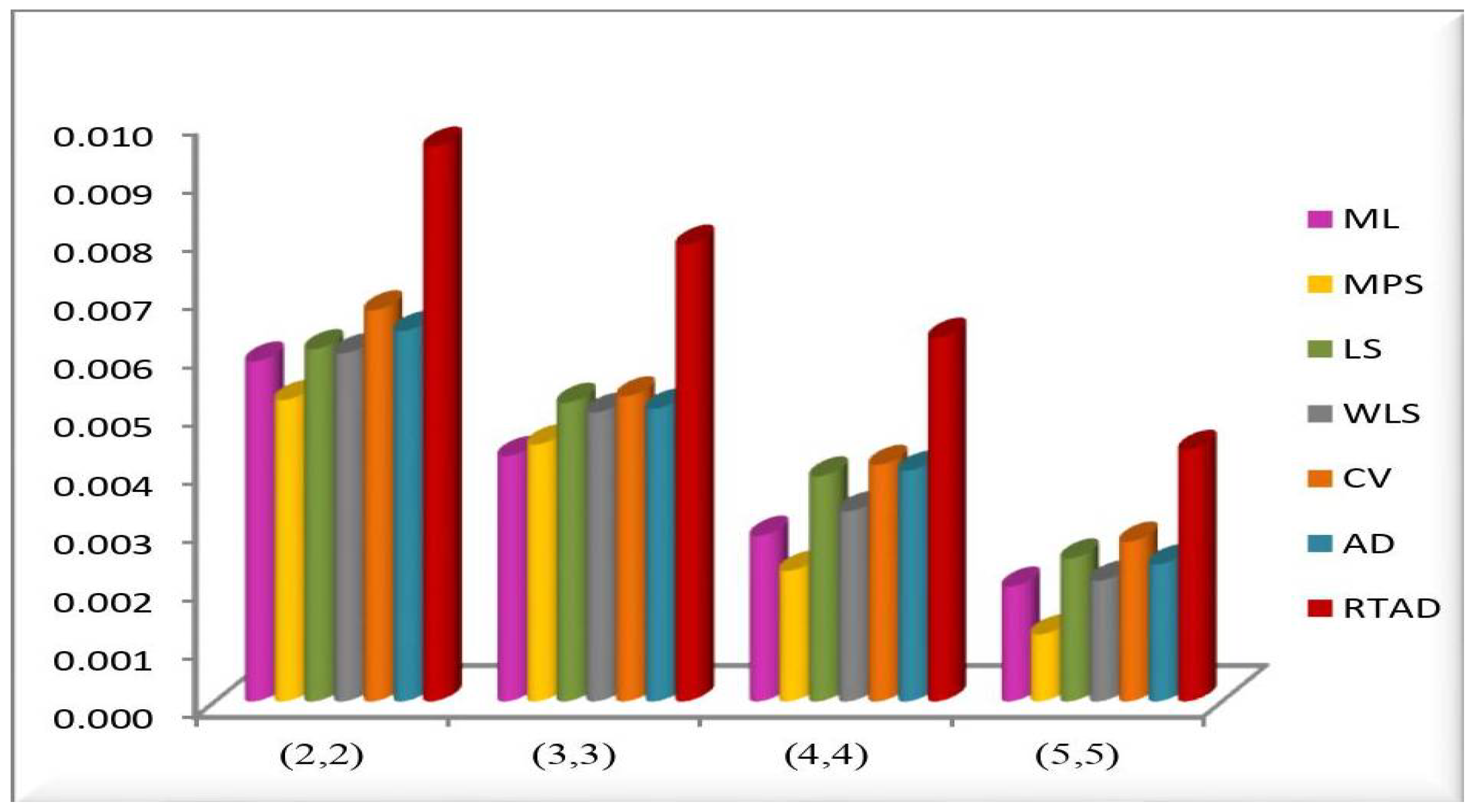
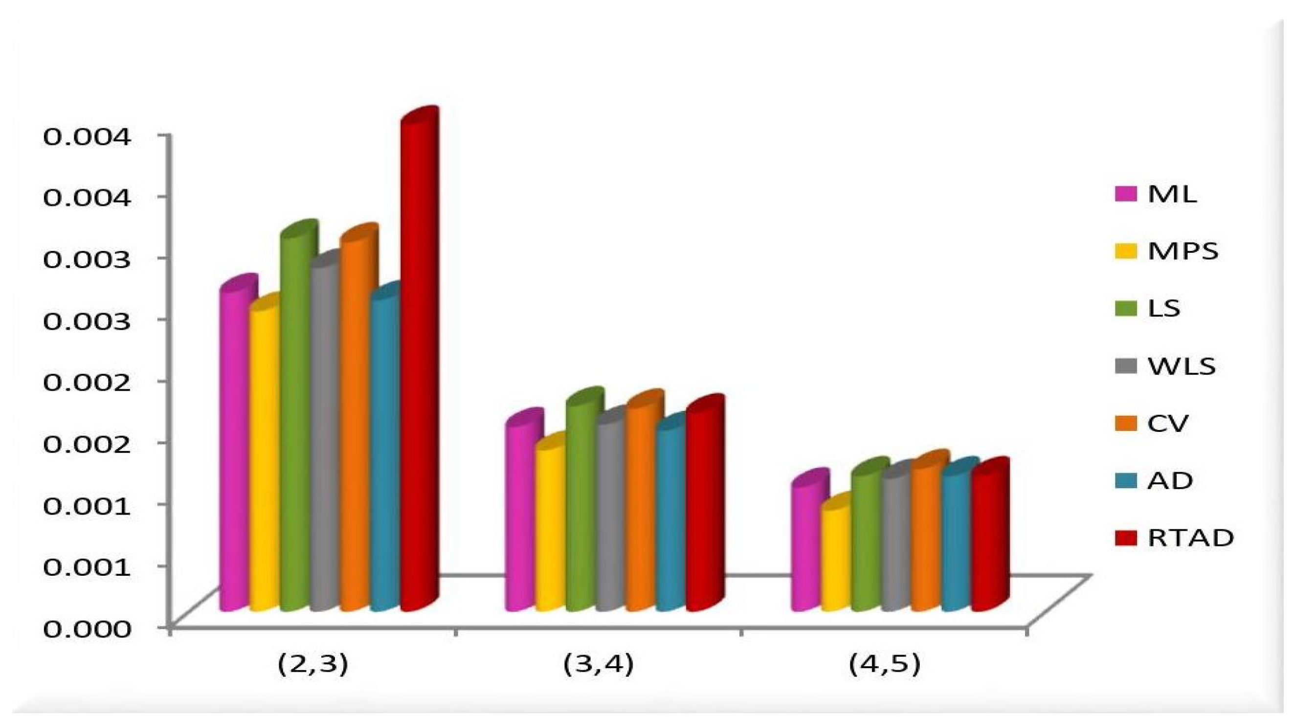
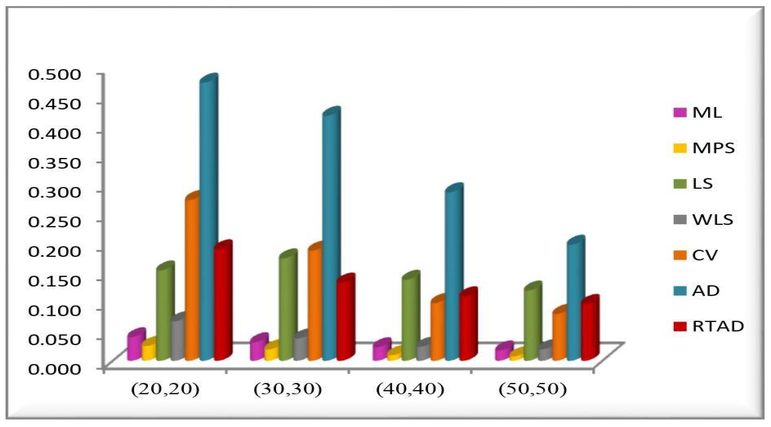
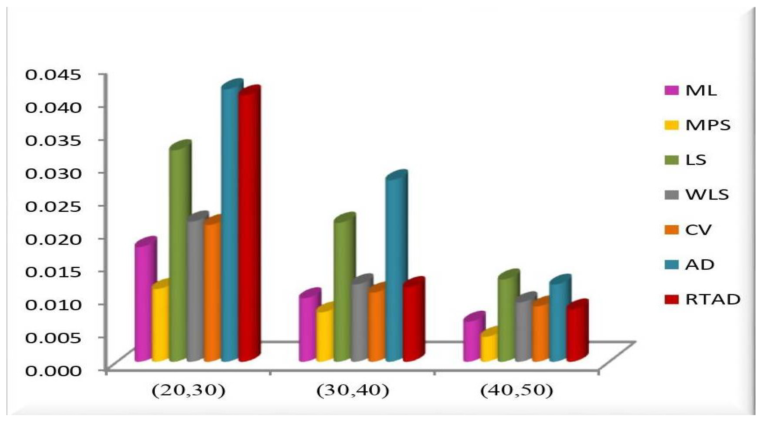
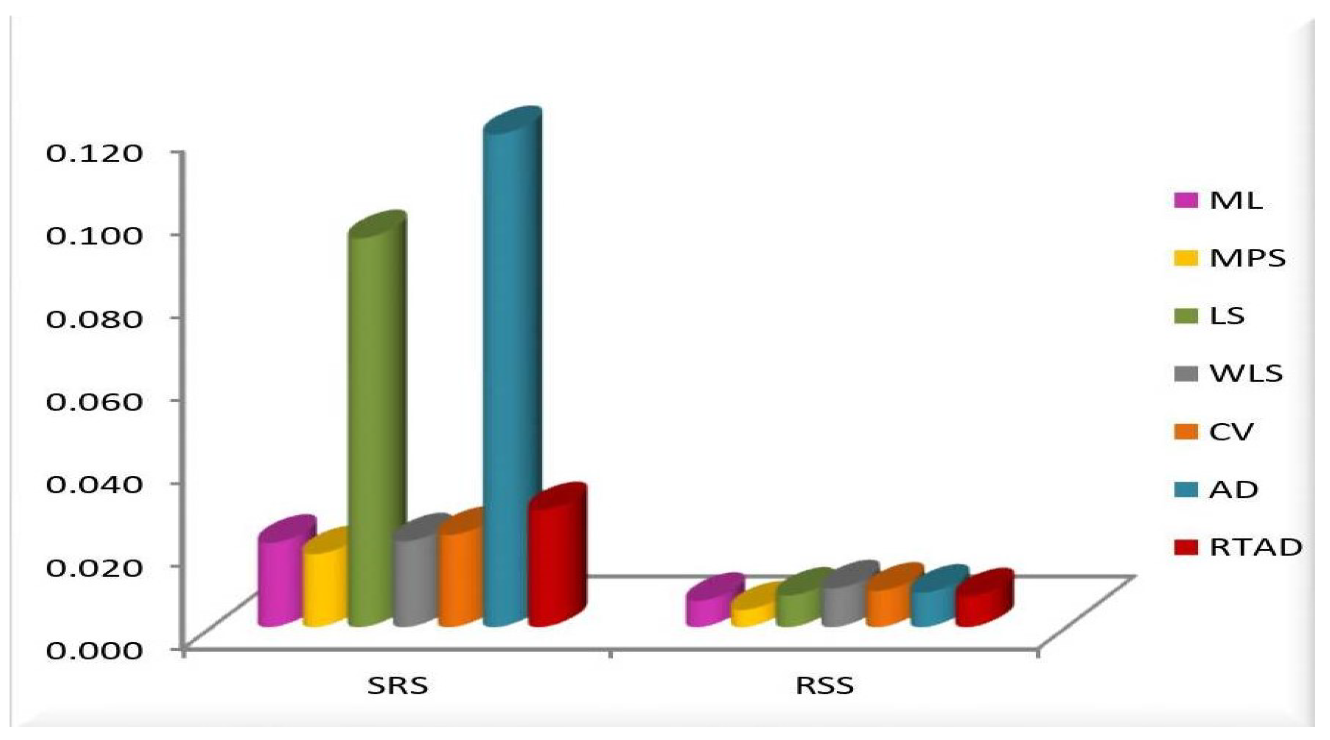
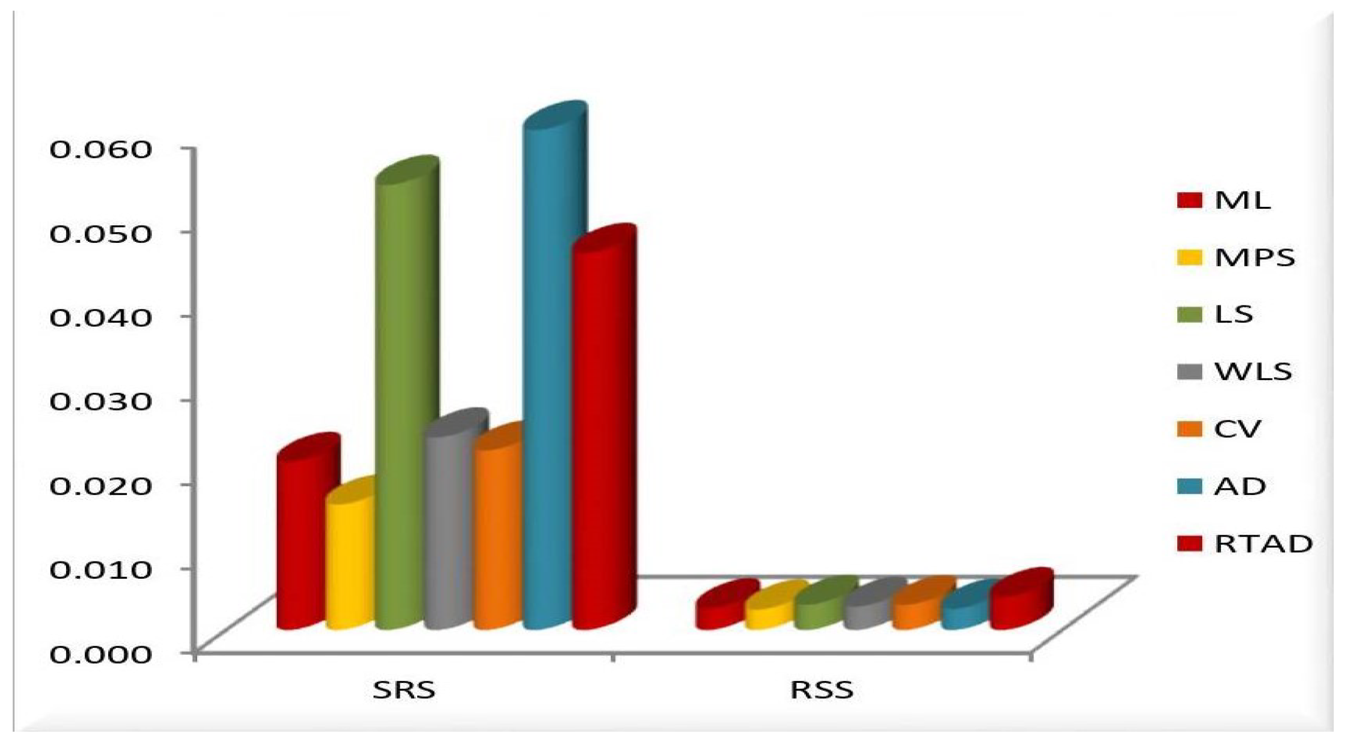
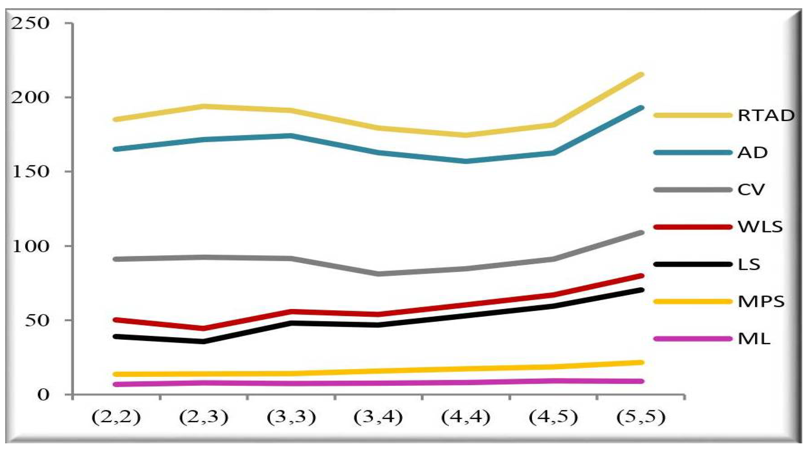
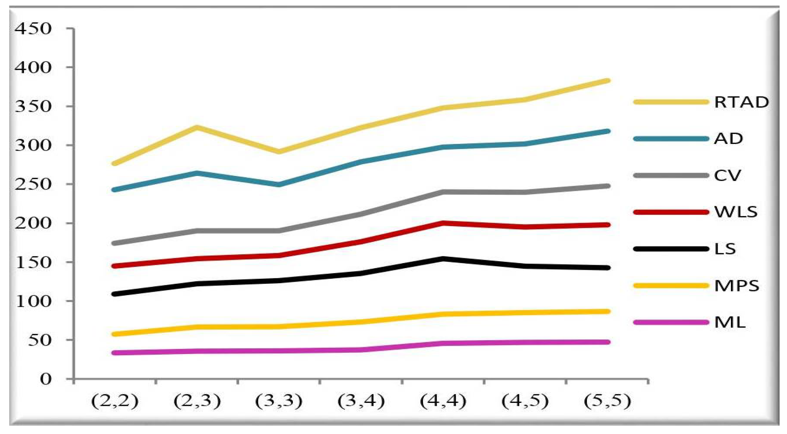
  • In the majority of the cases, as seen in Figure 2, the MSEs of the R estimates decrease as n w and n q increase.
  • The MSE of the R estimates for the RTAD method has the highest values (see Figure 2 and Figure 3).
  • The MSE of the R estimates for the MPS method has the smallest values, as seen in Figure 2 and Figure 3.
  • In the majority of the time, the MSEs of the R estimates decrease as ( n 1 , n 2 ) increases, also the R estimates from the MPS method typically take the lowest values when using the SRS (see Table 2 and Figure 4 and Figure 5).
  • For both sampling methods, the MSEs of the R estimates for the MPS method have the lowest values. While the MSEs of the R estimates for the AD method take the highest values in the SRS, the highest values are given to the MSEs of the estimates for the RTAD method in the RSS scheme.
  • Figure 6 and Figure 7 show that the RSS is preferable to the SRS with respect to MSE measures in most cases.
  • Figure 8 and Figure 9 show that the RTAD is the most efficient method for R at the true values R = 0.2857 , 0.9375 and a w = a q = 10 .
  • The RE increases as n w and n q increase (Figure 8 and Figure 9).
  • The MSE always decreases as n w and n q increase, indicating that the estimates are all consistent.
  • The estimates become more accurate as n 1 and n 2 increase, indicating that they are asymptotically unbiased.
  • The MSE always decreases as the true value of R increases, indicating that the estimates are all consistent.

7. Real Data Applications

Two data sets that ref. [55] proposed were considered in this section. The data collection includes two groups of head and neck cancer patients. The survival times of 58 head and neck cancer patients treated with radiation are shown in the data set for the first group, whereas the survival times of 44 patients treated with radiotherapy plus chemotherapy are shown in the data set for the second group. The information is as follows:
Data set I ( W ): 523, 583, 594, 14.48, 16.1, 22.7, 34, 41.55, 42, 45.28, 49.4, 84, 91, 160, 160, 165, 108, 112, 129, 133, 133, 139, 140, 140, 146, 149, 154, 157, 146, 149, 154, 157, 160, 160, 165, 173, 176, 218, 6.53, 7, 10.42, 225, 241, 248, 273, 277, 297, 405, 417, 53.62, 63, 64, 83, 420, 440, 1101, 1146, 1417.
Data set II ( Q ): 25.87, 31.98, 37, 41.35, 47.38, 55.46, 58.36, 63.47, 319, 339, 432, 469, 68.46, 78.26, 173, 179, 194, 195, 74.47, 81.43, 84, 92, 519, 633, 725, 94, 110, 112, 119, 127, 130, 133, 140, 146, 12.2, 23.56, 23.74, 155, 159, 209, 249, 281, 817, 1776.
We divide the data by 2000 to have values between 0 and 1. The Kolmogorov-Smirnov (K-S) goodness-of-fit test is used to fit each of the two data sets individually using the UGD. The UGD fits the data sets, according to the K-S test (K-ST) and the accompanying p-value. It is noted that for Data sets I and II, the K-ST of the UGD has values of 0.16913 and 0.070689, respectively, with p-values of 0.07245 and 0.9694.
The initial PDF shapes are reported utilizing the non-parametric kernel density estimation approach in Figure 10 and Figure 11 for both data sets. From Figure 10 and Figure 11, we can see that the shape of the PDF is asymmetric for both data sets. The normality condition is checked via the QQ plot; see Figure 10 and Figure 11. The outliers can also be spotted using the box plot; see Figure 10 and Figure 11. Henceforth, we can say that there are outliers in both data sets. Figure 12 and Figure 13 display the estimated CDF (ECDF), estimated PDF (EPDF), PP—plots, and estimated survival function (ESF) for the UGD. Thanks to its asymmetric properties, the UGD is an appropriate model for fitting these data.
In the earlier sections, it was assumed that stress and strength random variables followed the UGD with the same scale parameter and that the estimates of R were then examined. Consequently, in order to estimate it using actual data, we also need to see if the specifications of their second scale are the same.
First, it is assumed that W U G D ( τ 1 , φ 1 ) and Q U G D ( τ 2 , φ 2 ) . We perform the following tests of the hypothesis: H 0 : φ 1 = φ 2 vs H 1 : φ 1 φ 2 .
The associated likelihood function, based on the SRS, is given by:
L 1 ( τ 1 , φ 1 , τ 2 , φ 2 ) = l 1 = 1 n 1 τ 1 φ 1 w l 1 φ 1 1 exp τ 1 w l 1 φ 1 1 × l 2 = 1 n 2 τ 2 φ 2 q l 2 φ 2 1 exp τ 2 q l 2 φ 2 1 .
The MLEs of τ 1 , φ 1 , τ 2 and φ 2 are as follows: τ ^ 1 = 0 . 11552 , φ ^ 1 = 0 . 33684 , τ ^ 2 = 1 . 11884 and φ ^ 2 = 0 . 48394 , and the log-likelihood value is log L 1 ( τ 1 , φ 1 , τ 2 , φ 2 ) = 68 . 040 .
Second, suppose that W U G D ( τ 1 , φ ) and Q U G D ( τ 2 , φ ) , also, as the same steps in the above, the corresponding LF is given by:
L 2 ( τ 1 , τ 2 , φ ) = l 1 = 1 n 1 τ 1 φ w l 1 φ 1 exp τ 1 w l 1 φ 1 × l 2 = 1 n 2 τ 2 φ q l 2 φ 1 exp τ 2 q l 2 φ 1 .
The MLEs of τ 1 , τ 2 and φ are as follows: τ ^ 1 = 0 . 23668 τ ^ 2 = 0 . 18232 and φ ^ = 0 . 22347 and the log-likelihood value is log L 2 ( τ 1 , τ 2 , φ ) = 68 . 223 .
Then the likelihood ratio statistic is constructed as follows:
L R = 2 log L 2 ( τ 1 , τ 2 , φ ) L 1 ( τ 1 , φ 1 , τ 2 , φ 2 ) ,
that is, 2 log L 2 ( τ 1 , τ 2 , φ ) log L 1 ( τ 1 , φ 1 , τ 2 , φ 2 ) = 0.366 . As a result, the null hypothesis cannot be rejected. Therefore, in this case, the assumption of φ 1 = φ 2 is justified. Thus, both tests accept the null hypothesis that each data set is drawn from the UGD with the same scale parameter.
Then, using the suggested estimating methods for real data sets, we acquire various estimates of R . We observe that the MPS method cannot be used to estimate the parameters and reliability of Data set I because they have equal values D j 1 ( τ 1 ) = G ( w ( j 1 : n 1 ) ) G ( w ( j 1 1 : n 1 ) ) , D i 1 ( τ 1 ) = G ( w ( i 1 ) ) G ( w ( i 1 1 ) ) , i 1 = 1 , , n 1 based on the strength W, are equal to zero at most observation in both RSS and SRS. A similar observation is found for the second data set. Thus, different methods of estimation under different criteria are used to determine the estimated parameters, CV test (CVT), AD test (ADT), K-ST, and p-values for the proposed model. They are presented in Table 4 and Table 5 for the two real data sets, respectively. Therefore, the only estimates in Table 4 and Table 5 are the ML, LS, WLS, CV, AD, and RTAD estimates.
From these data, we suppose a SRS of size ( n 1 , n 2 ) = ( 20 , 20 ) , whereas for the RSS, a small set size of ( n w , n q ) = ( 2 , 2 ) is considered with cycles count being a w = a q = 10 . It is interesting to observe that the RSS and SRS are contrasted using the same quantity of measurement units. We determine the estimates of the parameters and reliability in each design using the preceding techniques with a perfect ranking. We use the previous criteria measures, i.e., CVT, ADT, K-ST, and p-value, to compare the different estimates from the two data sets.
The findings in Table 4 and Table 5 illustrate that the R estimates, via the RSS, are better than their equivalents in the SRS in terms of the smallest values of CVT, ADT, K-ST, and largest values of P–values, using the ML, LS, WLS, CV, AD, and RTAD methods.

8. Summary and Conclusions

In this paper, various estimation techniques for estimating the S-S reliability when both stress and strength random variables have the unit Gompertz distribution based on the RSS and SRS are covered. The methods that have been suggested include the maximum likelihood, least squares, weighted least squares, maximum product spacing, Cramér–von Mises, Anderson–Darling, and right tail Anderson–Darling methods. To assess the effectiveness of the proposed estimates based on both sampling designs, a simulation research is conducted. According to the results, for all the estimating techniques taken into consideration, the RSS estimates outperform the SRS estimates in terms of MSE, absolute bias, and efficiency values. The estimates based on the MPS have the smallest MSE for both sampling techniques. The reliability estimates based on the AD and RTAD methods have the largest MSE based on the SRS and RSS, respectively. Two real data sets that indicate the survival times of head and neck cancer patients have been used to provide further findings. Future research might look at the inference in a multicomponent S-S model based on the different RSS modifications.

Author Contributions

Conceptualization, N.A., A.S.H., M.E., C.C. and R.E.M.; methodology, N.A., A.S.H., M.E., C.C. and R.E.M.; software, N.A., A.S.H., M.E., C.C. and R.E.M.; validation, N.A., A.S.H., M.E., C.C. and R.E.M.; formal analysis, N.A., A.S.H., M.E., C.C. and R.E.M.; investigation, N.A., A.S.H., M.E., C.C. and R.E.M.; writing—original draft preparation, N.A., A.S.H., M.E., C.C. and R.E.M.; writing—review and editing, N.A., A.S.H., M.E., C.C. and R.E.M.; visualization, N.A., A.S.H., M.E., C.C. and R.E.M.; funding acquisition, N.A. All authors have read and agreed to the published version of the manuscript.

Funding

This research was funded by King Saud University, grant number RSPD2023R548.

Data Availability Statement

Not applicable.

Acknowledgments

Researchers Supporting Project number (RSPD2023R548), King Saud University, Riyadh, Saudi Arabia.

Conflicts of Interest

The authors declare no conflict of interest.

References

  1. Mazucheli, J.; Menezes, A.F.B.; Dey, S. The unit-Birnbaum–Saunders distribution with applications. Chil. J. Stat. 2018, 9, 47–57. [Google Scholar]
  2. Mazucheli, J.; Menezes, A.F.B.; Fernandes, L.B.; de Oliveira, R.P.; Ghitany, M.E. The unit-Weibull distribution as an alternative to the Kumaraswamy distribution for the modeling of quantiles conditional on covariates. J. Appl. Stat. 2020, 47, 954–974. [Google Scholar] [CrossRef]
  3. Mazucheli, J.; Menezes, A.F.B.; Dey, S. Unit-Gompertz distribution with applications. Stat. J. Appl. Stat. 2019, 79, 25–43. [Google Scholar]
  4. Ghitany, M.E.; Mazucheli, J.; Menezes, A.F.B.; Alqallaf, F. The unit-inverse Gaussian distribution: A new alternative to two-parameter distributions on the unit interval. Commun. Stat. Theory Methods 2019, 48, 3423–3438. [Google Scholar] [CrossRef]
  5. Korkmaz, M.C.; Chesneau, C. On the unit Burr-XII distribution with the quantile regression modeling and applications. Comput. Appl. Math. 2021, 40, 29. [Google Scholar] [CrossRef]
  6. Bantan, R.A.R.; Jamal, F.; Chesneau, C.; Elgarhy, M. Theory and applications of the unit Gamma/Gompertz distribution. Mathematics 2021, 9, 1850. [Google Scholar] [CrossRef]
  7. Bhatti, F.A.; Ali, A.; Hamedani, G.G.; Korkmaz, M.; Ahmad, M. The unit generalized log Burr XII distribution: Properties and application. AIMS Math. 2021, 6, 10222–10252. [Google Scholar] [CrossRef]
  8. Hassan, A.S.; Fayomi, A.; Algarni, A.; Almetwally, E.M. Bayesian and non-Bayesian inference for unit-exponentiated half-logistic distribution with data analysis. Appl. Sci. 2022, 12, 11253. [Google Scholar] [CrossRef]
  9. Khaoula, A.; Dey, S.; Kumar, D.; Seddik-Ameur, N. Different classical methods of estimation and chi-squared goodness-of-fit test for unit generalized inverse Weibull distribution. Austrian J. Stat. 2021, 50, 77–100. [Google Scholar] [CrossRef]
  10. Ribeiro, T.F.; Peña-Ramírez, F.A.; Guerra, R.R.; Cordeiro, G.M. Another unit Burr XII quantile regression model based on the different reparameterization applied to dropout in Brazilian undergraduate courses. PLoS ONE 2022, 17, e0276695. [Google Scholar] [CrossRef] [PubMed]
  11. Hashmi, S.; ul-Haq, M.A.; Zafar, J.; and Khaleel, M.A. Unit Xgamma Distribution: Its Properties, Estimation and Application. Proc. Pak. Acad. Sci. 2022, 59, 49–59. [Google Scholar] [CrossRef]
  12. Chesneau, C. A note on an extreme left skewed unit distribution: Theory, modelling and data fitting. Open Stat. 2021, 2, 1–23. [Google Scholar] [CrossRef]
  13. Fayomi, A.; Hassan, A.S.; Baaqeel, H.M.; Almetwally, E.M. Bayesian inference and data analysis of the unit-power Burr X distribution. Axioms 2023, 12, 297. [Google Scholar] [CrossRef]
  14. Hassan, A.S.; Alharbi, R.S. Different estimation methods for the unit inverse exponentiated Weibull distribution. Commun. Stat. Appl. Meth. 2023, 30, 191–213. [Google Scholar] [CrossRef]
  15. Korkmaz, M.Ç.; Korkmaz, Z.S. The unit log–log distribution: A new unit distribution with alternative quantile regression modeling and educational measurements applications. J. Appl. Stat. 2023, 50, 889–908. [Google Scholar] [CrossRef] [PubMed]
  16. Jha, M.K.; Dey, S.; Alotaibi, R.M.; Alomani, G.; Tripathi, Y.M. Reliability estimation of a multicomponent stress-strength model for unit Gompertz distribution under progressive Type II censoring. Qual. Reliab. Eng. Inter. 2020, 36, 965–987. [Google Scholar] [CrossRef]
  17. Jha, M.K.; Dey, S.; Tripathi, Y. Reliability estimation in a multicomponent stress-strength based on unit-Gompertz distribution. Inter. J. Qual. Reliab. Manag. 2019, 37, 428–450. [Google Scholar] [CrossRef]
  18. Kumar, D.; Dey, S.; Ormoz, E.; MirMostafaee, S.M.T.K. Inference for the unit-Gompertz model based on record values and inter-record times with an application. Rend. Circ. Mat. Palermo Ser. 2 2020, 69, 1295–1319. [Google Scholar] [CrossRef]
  19. Arshada, M.; Azhadc, Q.J.; Gupta, N.; Pathake, A.K. Bayesian inference of Unit Gompertz distribution based on dual generalized order statistics. Commun. Stat. Simul. Comput. 2021, 1–19. [Google Scholar] [CrossRef]
  20. McIntyre, G.A. A method for unbiased selective sampling, using ranked sets. Aust. J. Agric. Res. 1952, 3, 385–390. [Google Scholar] [CrossRef]
  21. Takahasi, K.W. On unbiased estimates of the population mean based on the sample stratified by means of ordering. Ann. Inst. Stat. Math. 1968, 21, 249–255. [Google Scholar] [CrossRef]
  22. Dell, D.R.; Clutter, J.L. Ranked set sampling theory with order statistics background. Biometrics 1972, 28, 545–555. [Google Scholar] [CrossRef]
  23. Wolfe, D.A. Ranked Set Sampling: Its Relevance and Impact on Statistical Inference. Int. Sch. Res. Not. Probab. Stat. 2012, 1–32. [Google Scholar] [CrossRef]
  24. Halls, L.K.; Dell, T.R. Trial of ranked-set sampling for forage yields. For. Sci. 1966, 12, 22–26. [Google Scholar]
  25. Stokes, S.L.; Sager, T.W. Characterization of a ranked-set sample with application to estimating distribution functions. J. Am. Stat. Assoc. 1988, 83, 374–381. [Google Scholar] [CrossRef]
  26. Johnson, G.D.; Paul, G.P.; Sinha, A.K. Ranked set sampling for vegetation research. Abstr. Bot. 1993, 17, 87–102. [Google Scholar]
  27. Gore, S.D.; Patil, G.P.; Sinha, A.K. Environmental Chemistry, Statistical Modeling, and Observational Economy. In Environmental Statistics, Assessment, and Forecasting; Cothern, C.R., Ross, N.P., Eds.; Lewis Publishing/CRC Press: Boca Raton, FL, USA, 1994; pp. 57–97. [Google Scholar]
  28. Al-Saleh, M.F.; Al-Shrafat, K. Estimation of milk yield using ranked set sampling. Envirometrics 2001, 12, 395–399. [Google Scholar] [CrossRef]
  29. Al-Saleh, M.F.; Al-Omari, A.I. Multistage ranked set sampling. J. Stat. Plann. Inference 2002, 102, 273–286. [Google Scholar] [CrossRef]
  30. Husby, C.E.; Stansy, E.A.; Wolfe, D.A. An application of ranked set sampling for mean and median estimation using USDA crop production data. J. Agric. Biolog. Environ. Stat. 2005, 10, 354–373. [Google Scholar] [CrossRef]
  31. Kowalczyk, B. Alternative sampling designs some applications of qualitative data in survey sampling. Stat. Trans. 2005, 7, 427–443. [Google Scholar]
  32. Ganeslingam, S.; Ganesh, S. Ranked set sampling versus simple random sampling in the estimation of the mean and the ratio. J. Stat. Manag. Syst. 2006, 2, 459–472. [Google Scholar] [CrossRef]
  33. Wang, Y.G.; Ye, Y.; Milton, D.A. Efficient designs for sampling and subsampling in fisheries research based on ranked sets. J. Marine Sci. 2009, 66, 928–934. [Google Scholar] [CrossRef]
  34. Kotz, S.; Lumelskii, Y.; Pensky, M. The Stress-Strength Model and Its Generalizations: Theory and Applications; World Scientific: Singapore, 2003. [Google Scholar]
  35. Birnbaum, Z.W. On a use if Mann-Whitney statistics. Proc. Third Berkeley Symp. Math. Stat. Probab. 1956, 1, 1317. [Google Scholar]
  36. Kundu, D.; Gupta, R.D. Estimation of P(Y < X) for Weibull distribution. IEEE Trans. Reliab. 2006, 55, 270–280. [Google Scholar]
  37. Raqab, M.Z.; Madi, M.D.; Kundu, D. Estimation of P(Y < X) for the 3-parameter generalized exponential distribution. Commun. Stat. Theory Meth. 2008, 37, 2854–2864. [Google Scholar]
  38. Asgharzadeh, A.; Valiollahi, R.; Raqab, M.Z. Estimation of Pr(Y < X) for the two-parameter generalized exponential records. Commun. Stat. Simul. Comput. 2017, 46, 371–394. [Google Scholar]
  39. Nadeb, H.; Torabi, H.; Zhao, Y. Stress-strength reliability of exponentiated Fréchet distributions based on Type-II censored data. J. Stat. Comput. Simul. 2019, 89, 1863–1876. [Google Scholar] [CrossRef]
  40. Muttlak, H.A.; Abu-Dayyeh, W.A.; Saleh, M.F.; Al-Sawi, E. Estimating P(Y < X) using ranked set sampling in case of the exponential distribution. Commun. Stat. Theory Methods 2010, 39, 1855–1868. [Google Scholar]
  41. Akgül, F.G.; Şenoğlu, B. Estimation of P (X < Y) using ranked set sampling for the Weibull distribution. Qual. Technol. Quant. Manag. 2017, 14, 296–309. [Google Scholar]
  42. Akgül, F.G.; Acıtaş, Ş.; Şenoğlu, B. Inferences on stress-strength reliability based on ranked set sampling data in case of Lindley distribution. J. Stat. Comput. Simul. 2018, 88, 3018–3032. [Google Scholar] [CrossRef]
  43. Akgül, F.G.; Acıtaş, Ş.; Şenoğlu, B. Inferences for stress-strength reliability of Burr Type X distributions based on ranked set sampling. Commun. Stat. Simul. Comput. 2022, 51, 3324–3340. [Google Scholar] [CrossRef]
  44. Esemen, M.; Gurler, S.; Sevinc, B. Estimation of stress-strength reliability based on ranked set sampling for generalized exponential distribution. Int. J. Reliab. Qual. Saf. Eng. 2021, 28, 2150011. [Google Scholar] [CrossRef]
  45. Hassan, A.S.; Al-Omari, A.I.; Nagy, H.F. Stress-Strength reliability for the generalized inverted exponential distribution using MRSS. Iran. J. Sci. Technol. Trans. A Sci. 2021, 45, 641–659. [Google Scholar] [CrossRef]
  46. Al-Omari, A.I.; Hassan, A.S.; Alotaibi, N.; Shrahili, M.; Nagy, H.F. Reliability estimation of inverse Lomax distribution using extreme ranked set sampling. Adv. Math. Phys. 2021, 2021, 4599872. [Google Scholar] [CrossRef]
  47. Yousef, M.M.; Hassan, A.S.; Al-Nefaie, A.H.; Almetwally, E.M.; Almongy, H.M. Bayesian estimation using MCMC method of system reliability for inverted Topp-Leone distribution based on ranked set sampling. Mathematics 2022, 10, 3122. [Google Scholar] [CrossRef]
  48. Hassan, A.S.; Elshaarawy, R.S.; Onyango, R.; Nagy, H.F. Estimating system reliability using neoteric and median RSS data for generalized exponential distribution. Int. J. Math. Math. Sci. 2022, 2022, 2608656. [Google Scholar] [CrossRef]
  49. Yahya, M.; Shaaban, M. Estimation of stress-strength reliability from exponentiated inverse Rayleigh Rayleigh distribution based on neoteric ranked set sampling approach. Pak. J. Stat. 2022, 38, 491–511. [Google Scholar]
  50. Hassan, A.S.; Almanjahie, I.M.; Al-Omari, A.I.; Alzoubi, L.; Nagy, H.F. Stress- strength modeling using median-ranked set sampling: Estimation, simulation, and application. Mathematics 2023, 11, 318. [Google Scholar] [CrossRef]
  51. Hassan, A.S.; Alsadat, N.; Elgarhy, M.; Chesneau, C.; Nagy, H.F. Analysis of R = P[Y < X < Z] using ranked set sampling for a generalized inverse exponential model. Axioms 2023, 12, 302. [Google Scholar]
  52. Swain, J.; Venkatraman, S.; Wilson, J. Least squares estimation of distribution function in Johnson’s translation system. J. Stat. Comput. Simul. 1988, 29, 271–297. [Google Scholar] [CrossRef]
  53. Cheng, R.C.H.; Amin, N.A.K. Estimating parameters in continuous univariate distributions with a shifted origin. J. R. Stat. Soc. 1983, 45, 394–403. [Google Scholar] [CrossRef]
  54. Ranneby, B. The maximum spacing method: An estimation method related to the maximum likelihood method. Scand. J. Stat. 1984, 11, 93–112. [Google Scholar]
  55. Efron, B. Logistic regression, survival analysis, and the Kaplan-Meier curve. J. Am. Stat. Assoc. 1988, 83, 414–425. [Google Scholar] [CrossRef]
Figure 1. Various plots of the PDF (subfigure (a)) and HF (subfigure (b)) of the UGD.
Symmetry 15 01121 g001
Figure 2. MSE of the R estimates for all the methods at R = 0.60000 in the RSS.
Symmetry 15 01121 g002
Figure 3. MSE of the R estimates for all the methods at R = 0.71430 in the RSS.
Symmetry 15 01121 g003
Figure 4. MSE of the R estimates for all the methods at R = 0.28570 in the SRS.
Symmetry 15 01121 g004
Figure 5. MSE of the R estimates for all the methods at R = 0.93750 in the SRS.
Symmetry 15 01121 g005
Figure 6. MSE of the R estimates for all the methods at ( n w , n q ) = ( 4 , 4 ) , ( n 1 , n 2 ) = ( 40 , 40 ) and R = 0.60000 .
Symmetry 15 01121 g006
Figure 7. MSE of the R estimates for all the methods at ( n w , n q ) = ( 2 , 3 ) , ( n 1 , n 2 ) = ( 20 , 30 ) and R = 0.71430 .
Symmetry 15 01121 g007
Figure 8. RE of the R estimates at R = 0.28570 for different ( n w , n q ) at a w = a q = 10 .
Symmetry 15 01121 g008
Figure 9. RE of the R estimates at R = 0.93750 for different ( n w , n q ) at a w = a q = 10.
Symmetry 15 01121 g009
Figure 10. Some basic non-parametric plots for Data set I.
Symmetry 15 01121 g010
Figure 11. Some basic non-parametric plots for Data set II.
Symmetry 15 01121 g011
Figure 12. ECDF, EPDF, PP plots and ESF of the UGD for Data set I.
Symmetry 15 01121 g012
Figure 13. ECDF, EPDF, PP plots and ESF of the UGD for Data set II.
Symmetry 15 01121 g013
Table 1. Measures of different R estimates for the UGD under the RSS.
R ( n w , n q ) ( n 1 , n 2 ) RSS
MeasuresMLMPSLSWLSCVADRTAD
0.28570(2,2)(20,20)AB0.009840.005260.008240.006450.007350.008420.00743
MSE0.005840.005180.006050.005980.006720.006360.00954
(2,3)(20,30)AB0.008650.005150.007640.005320.006340.008040.00694
MSE0.004840.004960.005730.005540.005820.005630.00832
(3,3)(30,30)AB0.007240.004560.006980.004860.005970.007840.00617
MSE0.004210.004410.005130.004960.005240.005030.00785
(3,4)(30,40)AB0.007360.004140.006150.004430.005240.007050.00585
MSE0.003840.003270.004750.004250.004950.004860.00715
(4,4)(40,40)AB0.006350.003850.005950.004190.004920.006740.00516
MSE0.002840.002240.003860.003260.004060.003960.00625
(4,5)(40,50)AB0.005740.003130.005530.003940.004210.006180.00497
MSE0.002140.001960.003140.002730.003740.003040.00535
(5,5)(50,50)AB0.005270.002650.004280.003160.004070.005440.00421
MSE0.001970.001150.002450.002070.002740.002350.00432
0.60000(2,2)(20,20)AB0.007430.004980.000720.000390.004340.000840.00583
MSE0.004770.00390.00540.004980.006110.004680.00783
(2,3)(20,30)AB0.007180.004020.000340.000320.003430.000270.00924
MSE0.003470.003030.003860.003740.004230.003450.00531
(3,3)(30,30)AB0.007220.001860.000350.000210.00110.00030.00356
MSE0.002350.002190.002620.00240.002810.002350.00345
(3,4)(30,40)AB0.006620.00380.000260.000850.003140.000250.0044
MSE0.001860.001740.002110.001970.002250.001890.00287
(4,4)(40,40)AB0.001490.004370.000140.000220.0010.000120.00215
MSE0.001180.001250.001460.001360.001580.001290.00167
(4,5)(40,50)AB0.000990.009720.00280.002360.000110.00320.00189
MSE0.000940.000860.001280.00120.000950.001190.0011
(5,5)(50,50)AB0.001190.003550.000110.000110.000980.00010.00316
MSE0.000750.000710.00110.0010.001070.000990.00097
0.71430(2,2)(20,20)AB0.008650.001220.000290.002060.008870.000120.00815
MSE0.003850.003540.004220.003960.004650.00380.00578
(2,3)(20,30)AB0.006560.001370.001180.002040.008230.000120.00952
MSE0.002590.002440.003030.002790.0030.002530.00395
(3,3)(30,30)AB0.002160.001430.001580.000010.004480.002570.0043
MSE0.001850.001630.00190.001780.002050.001650.0022
(3,4)(30,40)AB0.002270.013190.00210.001140.002880.002480.00254
MSE0.00150.001310.001670.001520.001650.001470.00161
(4,4)(40,40)AB0.008620.004870.002220.003380.006580.00110.00659
MSE0.00120.001140.001220.001240.001430.001230.0014
(4,5)(40,50)AB0.00250.001120.000640.001110.004710.000390.00569
MSE0.001010.000820.00110.001080.001160.00110.0011
(5,5)(50,50)AB0.002130.010590.00120.002210.004790.000120.00539
MSE0.000820.000630.000990.000840.000970.000840.00086
0.93750(2,2)(20,20)AB0.002740.001480.006460.004680.001280.004410.00191
MSE0.000770.000520.000930.000840.000830.000770.00127
(2,3)(20,30)AB0.001490.001290.006050.004530.000470.004110.00203
MSE0.000490.000360.000580.000660.000580.000560.00069
(3,3)(30,30)AB0.00150.001130.00480.003070.000460.003350.00168
MSE0.000340.00030.000480.000410.000380.000520.00046
(3,4)(30,40)AB0.000190.00110.004880.003680.000690.003380.00204
MSE0.000260.000210.000340.000290.00030.000410.00026
(4,4)(40,40)AB0.000940.009460.003650.00230.000340.002560.00083
MSE0.000150.000120.000270.000220.000250.000340.00017
(4,5)(40,50)AB0.001080.008550.003030.001830.000180.001840.00069
MSE0.000130.00010.000210.000180.000190.000190.00014
(5,5)(50,50)AB0.001630.007020.002470.001080.00070.001190.00015
MSE0.000090.000070.000180.000160.000160.000150.00011
Table 2. Measures of different R estimates for the UGD under the SRS.
R ( n 1 , n 2 ) SRS
MeasuresMLMPSLSWLSCVADRTAD
0.28570(20,20)AB0.175190.161740.703170.031570.260930.685450.27421
MSE0.040120.035290.15370.067340.27340.471930.18969
(20,30)AB0.01550.085330.006920.150860.062470.681190.03833
MSE0.037950.029630.12510.048910.278650.446830.1861
(30,30)AB0.011550.019640.004950.13090.046920.59670.02273
MSE0.031580.029530.174230.037950.187370.41590.13309
(30,40)AB0.007860.007380.003750.129960.010810.304580.01076
MSE0.029840.026380.146880.030570.134540.39660.11841
(40,40)AB0.005160.006280.001750.118650.010360.319730.01107
MSE0.023150.020570.137890.023950.098340.286430.10976
(40,50)AB0.004280.004160.004620.115790.009720.286630.01087
MSE0.019760.018630.127880.020640.090120.217270.10107
(50,50)AB0.003970.002670.002460.105460.001710.218650.01025
MSE0.017650.014560.119560.019650.079660.197530.09674
0.60000(20,20)AB0.160020.139420.389440.138810.129240.378390.2296
MSE0.034540.027220.152780.043060.053750.143730.07758
(20,30)AB0.157970.131290.380940.13090.126950.378260.21932
MSE0.033340.022790.111570.040750.042960.143440.06812
(30,30)AB0.156250.130650.357070.130.121060.373060.18365
MSE0.029320.021110.136720.033840.034060.139960.05182
(30,40)AB0.142540.129850.352020.121010.095390.372050.15646
MSE0.027690.020390.133880.0270.028690.134310.04696
(40,40)AB0.14790.115330.391350.153340.109490.385880.13785
MSE0.02040.017680.123390.020760.022340.118970.02834
(40,50)AB0.137470.110360.386230.148280.101070.375350.12876
MSE0.018870.015260.119630.019460.019740.112230.01936
(50,50)AB0.115560.107850.318770.128540.100960.327650.11876
MSE0.015050.012880.115460.016240.015830.110560.01758
0.71430(20,20)AB0.142970.129730.279830.170080.156360.23940.23269
MSE0.026380.019740.078330.032250.027960.061020.05619
(20,30)AB0.13220.117790.271760.122160.101260.245780.20279
MSE0.020060.014980.053960.022980.021450.051460.04489
(30,30)AB0.119590.126830.275590.128660.110890.24720.12942
MSE0.017650.012820.046020.015160.019540.041770.02913
(30,40)AB0.110960.119650.229870.120980.109440.228750.11987
MSE0.015880.010950.039870.013040.016980.038640.02226
(40,40)AB0.108750.112580.218770.118770.078610.215450.11543
MSE0.014990.009950.023970.010870.015150.032650.01995
(40,50)AB0.100870.109980.187630.102580.057890.209660.10976
MSE0.012680.007340.020650.009550.013410.029680.01592
(50,50)AB0.084460.056760.168680.086340.036680.184430.10025
MSE0.010860.005750.010650.007850.011350.022670.01299
0.93750(20,20)AB0.074360.091240.936980.118720.27610.876430.58189
MSE0.025770.012440.047940.030220.024260.052890.04265
(20,30)AB0.206560.225910.937330.246620.719680.93750.24549
MSE0.01750.01110.032170.021350.020840.041420.04047
(30,30)AB0.144050.207950.937250.437490.416080.983240.1437
MSE0.012260.009280.028440.013150.012110.030790.01935
(30,40)AB0.238870.321840.997430.612780.519330.987640.05003
MSE0.009680.007540.021170.011810.010560.027630.01138
(40,40)AB0.130430.234490.937310.24020.495190.93750.04162
MSE0.006840.00450.019220.010060.009990.019530.00854
(40,50)AB0.203970.273710.764490.220490.700240.845360.17623
MSE0.00610.003810.012540.009060.008450.011760.00796
(50,50)AB0.156770.214860.798760.284340.612790.875340.11587
MSE0.004250.002750.010080.008850.007950.010560.00715
Table 3. RE of different R estimates of the UGD.
R ( n w , n q ) ( n 1 , n 2 ) RE
MLMPSLSWLSCVADRTAD
0.28570(2,2)(20,20)6.869866.8180125.4049611.2608740.6845274.1678519.88365
(2,3)(20,30)7.840915.9737921.832468.8285247.8780179.365922.36779
(3,3)(30,30)7.501196.6961533.962967.6512135.7576382.683916.95414
(3,4)(30,40)7.770838.0672830.922117.1929427.179881.6049416.56084
(4,4)(40,40)8.151419.1830435.72287.345424.2216772.3308117.5616
(4,5)(40,50)9.233649.505140.726117.5604424.0962671.4696718.89234
(5,5)(50,50)8.9593912.6608748.801229.4927529.0740984.0553222.39398
0.60000(2,2)(20,20)7.241096.9794928.292598.646598.7970530.711549.90805
(2,3)(20,30)9.608077.5214528.9041510.8957210.1560341.5768112.82863
(3,3)(30,30)12.47669.6392752.1832114.1117612.12159.5574515.02029
(3,4)(30,40)14.887111.7183963.4502413.7055812.7511171.0634916.36237
(4,4)(40,40)17.2881414.14484.513715.2647114.1392492.2248116.92951
(4,5)(40,50)20.0744717.8479593.4640616.2183320.7821194.3142917.60364
(5,5)(50,50)20.1203218.23654104.9636416.24314.79215111.6767718.12062
0.71430(2,2)(20,20)6.851955.5762718.561618.143946.012916.057899.72145
(2,3)(20,30)7.745176.1381117.808588.236567.1520.3399211.36456
(3,3)(30,30)9.540547.8650324.221058.516859.5317125.3151513.24091
(3,4)(30,40)10.586678.3603123.875458.5809210.2884826.2857113.81141
(4,4)(40,40)12.48758.7280719.647548.762110.597226.5447214.24065
(4,5)(40,50)12.551498.9553718.775828.8379611.5637926.9814.47545
(5,5)(50,50)13.247569.1336510.760619.3488111.7010326.9921415.1
0.93750(2,2)(20,20)33.4675323.9230851.5483935.9702429.2301268.6883133.57953
(2,3)(20,30)35.7142930.8444455.456932.3515235.9326473.9696458.64638
(3,3)(30,30)36.0588230.9233359.2532.0756131.8552659.2098142.06522
(3,4)(30,40)37.2461535.9052462.2540.706935.2066767.3926843.78077
(4,4)(40,40)45.5933337.5183371.1977845.7409139.9657.4529450.23529
(4,5)(40,50)46.9230838.1459.7285750.3333344.4736861.8947456.88571
(5,5)(50,50)47.2666739.342865655.312549.7093870.3733364.96364
Table 4. Different estimates of τ 1 , τ 2 , φ and R for Data sets I and II under the RSS and SRS.
SamplingParameterMLLSWLSCVADRTAD
RSS τ 1 0.09850.03640.025020.019950.080080.01273
τ 2 0.06580.02150.014790.010950.05170.00782
φ 0.80611.19191.31581.423990.883021.57378
R 0.599540.628280.628440.645630.607680.61925
SRS τ 1 0.09990.052280.045010.010160.14420.006
τ 2 0.066540.029440.023610.005360.090.00367
φ 0.81191.057981.105821.60.692611.83009
R 0.600210.639780.655940.654530.615710.62078
Table 5. Goodness of fit measures by different estimation methods for Data sets I and II under the RSS and SRS.
DataMethodDesignCVTADTK-STp-Value
Data I
(W)
MLRSS0.313071.771290.802080.19792
SRS0.356761.971970.837530.16247
LSRSS0.582413.025930.595060.40494
SRS0.819774.032630.64420.3558
WLSRSS0.689883.514390.647090.35291
SRS0.858424.217980.667890.33211
CVRSS0.805074.034470.460130.5399
SRS1.195795.855610.82540.1746
ADRSS0.319751.806420.800610.19939
SRS0.460972.528280.804680.19532
RTADRSS0.922094.564460.542940.45706
SRS1.338126.50310.64110.3589
Data II
(Q)
MLRSS0.090680.520670.855940.14406
SRS0.116480.692090.928170.07183
LSRSS0.1778724.007540.448510.55149
SRS1.2051925.883310.891920.10808
WLSRSS0.2475524.411830.526570.47343
SRS1.2236226.327250.901680.09832
CVRSS0.3233724.826670.568850.43115
SRS0.5705325.141190.942040.05796
ADRSS0.0775923.393390.166220.83378
SRS0.1584523.912920.897780.10222
RTADRSS0.460012.582140.710770.28923
SRS0.789254.157390.945170.05483
Disclaimer/Publisher’s Note: The statements, opinions and data contained in all publications are solely those of the individual author(s) and contributor(s) and not of MDPI and/or the editor(s). MDPI and/or the editor(s) disclaim responsibility for any injury to people or property resulting from any ideas, methods, instructions or products referred to in the content.

