
The Modified-Lomax Distribution: Properties, Estimation Methods, and Application


Unit of Scientific Research, Applied College, Qassim University, Buraydah 51452, Saudi Arabia
Symmetry 2023, 15(7), 1367; https://doi.org/10.3390/sym15071367
Submission received: 9 June 2023
/
Revised: 26 June 2023
/
Accepted: 3 July 2023
/
Published: 5 July 2023
(This article belongs to the Special Issue Symmetry in Statistics and Data Science, Volume 2)
Abstract
:This paper introduces a flexible three-parameter extension of the Lomax model called the odd Lomax–Lomax (OLxLx) distribution. The OLxLx distribution can provide left-skewed, symmetrical, right-skewed, and reversed-J shaped densities and increasing, constant, unimodal, and decreasing hazard rate shapes. Some mathematical properties of the introduced model are derived. The OLxLx density can be expressed as mixture of Lomax densities. The OLxLx parameters are estimated by using eight estimation methods and their performance is explored by using detailed simulation studies. The partial and overall ranks of the mean relative errors, absolute biases, and mean square errors of different estimators are presented to choose the best estimation method. The flexibility and applicability of the OLxLx distribution is shown using real-life medicine data, illustrating the superior fit of the OLxLx distribution over other competing Lomax distributions. The OLxLX distribution outperforms some rival Lomax distributions including the Kumaraswamy–Lomax, McDonald–Lomax, Weibull–Lomax, transmuted Weibull–Lomax, exponentiated-Lomax, Lomax–Weibull, modified Kies–Lomax, Burr X Lomax, beta exponentiated-Lomax, odd exponentiated half-logistic Lomax, and transmuted-Lomax distributions, among others.
1. Introduction
The choice of appropriate distributions to be used on real-life data plays a fundamental role in improving the power, efficiency, and sensitivity of statistical tests. This is so because appropriate distributions lead to a good fit of the data. Therefore, good knowledge of the appropriate distribution to be used for a specific data set is essential.
Probability distributions are very important in data analysis. They can be used to model wide range of data shapes in applied fields. The Lomax (Lx) (also known as Pareto II) distribution has many applications in several applied areas such as income and wealth inequality, biological sciences, lifetime and reliability, engineering, and actuarial sciences. The Lx distribution has been applied in modeling real-life data in income and wealth, firm size, and reliability and life testing (see [1,2,3,4]). Chahkandi and Ganjali [5] showed that the Lx distribution belongs to decreasing hazard rate (HR) family. More information about the Lx distribution can be explored in [6,7,8].
The procedure of adding new shape parameters for generalizing classical distributions is a well-known technique in the statistical literature. Hence, there are several extensions of the Lx distribution which are developed using well-known families to improve its flexibility and applicability in modeling different types of data. For example, Gupta et al. [9] introduced the exponentiated-Lomax, the Marshall–Olkin Lomax was proposed by [10], the Kumaraswamy–Lomax by [11], the Weibull–Lomax was studied by [8], the exponentiated half logistic-Lomax was introduced by [12], the Fréchet Topp–Leone Lomax was proposed by [13], and the generalized linear failure rate Lomax by [14].
Recently, developing new generators of distributions by adding one or more extra shape parameters to the well-known distributions has received great interest among statisticians. One of the most notable families is called the odd Lomax-G (OLx-G) family, which was introduced by Cordeiro et al. [15].
In this paper, a new flexible three-parameter Lx extension called the odd Lomax–Lomax (OLxLx) distribution is introduced to improve the flexibility of the Lx distribution for modeling real-life data. The OLxLx distribution is generated by replacing the baseline one-parameter Lx distribution in the OLx-G family. The OLxLx distribution can provide better fit than fourteen existing competing Lx extensions which contain four or five parameters. The three-parameter OLxLx distribution provides constant, increasing, unimodal, decreasing, and reversed-J shaped failure rate functions, as well as left-skewed, symmetrical, right-skewed, and reversed-J shaped densities. Another important goal of this paper is to explore the estimation of the OLxLx parameters via several classical methods including the maximum likelihood, Cramér–von Mises, Anderson–Darling, least-squares, right-tail Anderson–Darling, weighted least-squares, maximum product of spacings, and percentiles based estimation methods. Furthermore, the performance of these estimation approaches is investigated using detailed simulation results based on the average values of mean square error (MSE), absolute biases (), and mean relative errors (MRE) of the estimates. Additionally, the three measures, MSE, , and MRE, are ordered based on partial and overall ranks in order to compare the performances of the introduced estimators as well as to determine the best estimation approach for the unknown parameters of the OLxLx distribution.
The rest of the paper is outlined as follows. The OLxLx distribution is presented in Section 2. In Section 3, the basic properties of the OLxLx distribution are determined. Eight estimation methods are explored in Section 4. Detailed simulations for the studied estimation methods are presented in Section 5. The applicability of the OLxLx model is studied using real-life data in Section 6. Finally, the conclusions are provided in Section 7.
2. The OLxLx Distribution
In this section, we define the OLxLx distribution based on the OLx-G family [15].
The cumulative distribution function (CDF) of the OLx-G family is defined (for ) by
The probability density function (PDF) of the OLx-G family reduces to
where . The OLx-G family reduces to the Marshall-Olkin-G (MO-G) family (Marshall and Olkin, [16]) for .
The HR function (HRF) of the OLx-G follows as
The quantile function (QF) of the OLx-G takes the form
where is the baseline QF of any G distribution and .
The one-parameter Lx distribution with shape parameter is specified by the CDF
The PDF of the Lx distribution reduces to
The survival function (SF) and HRF of the OLxLx distribution are given by
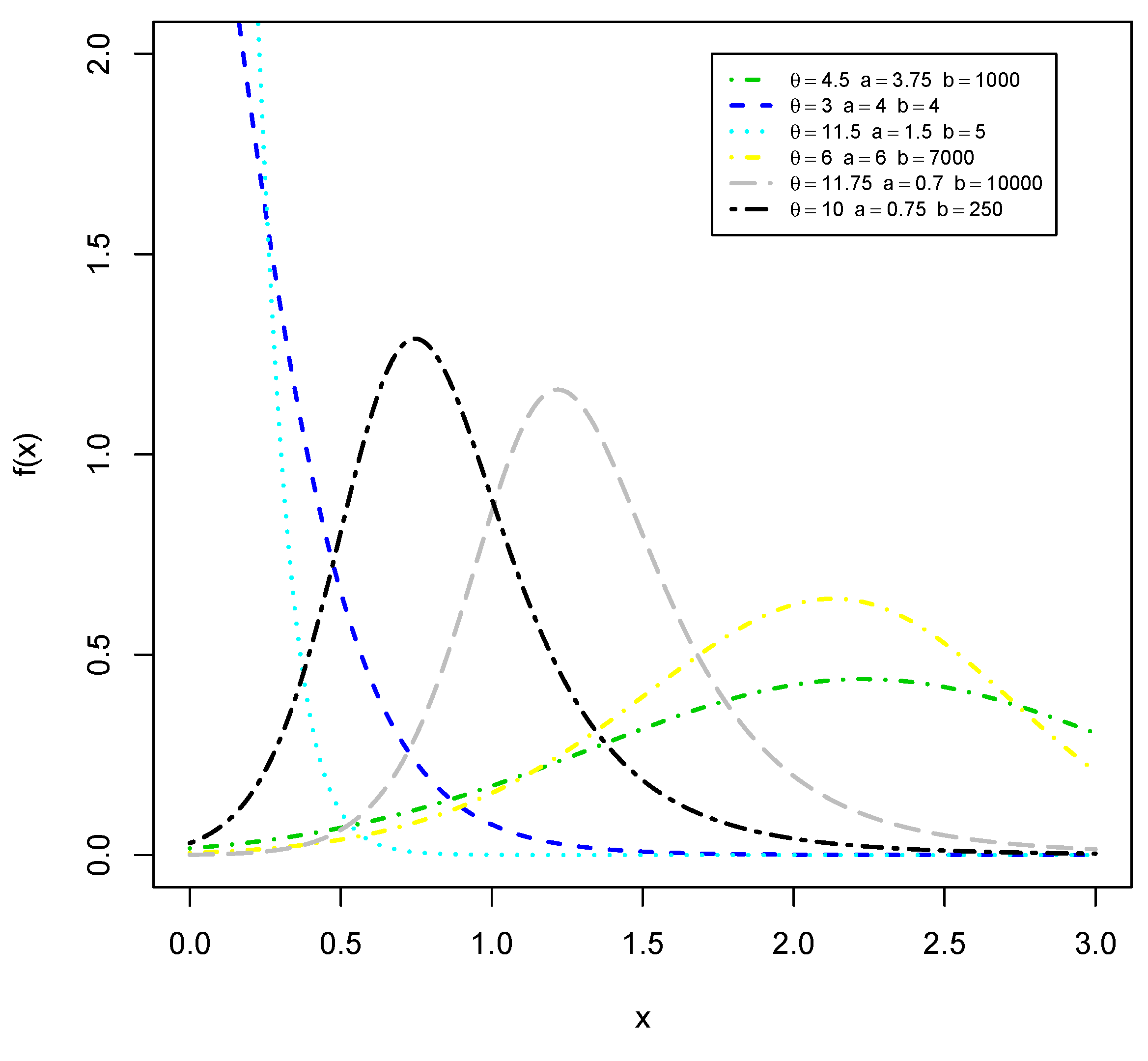
The two-parameter Marshall–Olkin Lomax (TPMOLx) distribution follows from (7) as a special case of the OLxLx distribution for . Possible shapes for the PDF and HRF of the OLxLx distribution are given in Figure 1 and Figure 2. The plots in these figures illustrate that the OLxLx distribution can provide symmetrical, right-skewed, left-skewed, and J shaped densities. Furthermore, the OLxLx HRF can be constant, increasing, decreasing, and unimodal shaped.
3. Mathematical Properties
This section provides some statistical properties of the newly introduced model.
3.1. Linear Expansion
A useful linear mixture representation for the PDF (7) of the OLxLx distribution is derived. Cordeiro et al. [15] provided a linear representation of the OLx-G CDF (2) as follows
where
and denotes the exponentiated-G (Exp-G) family density with power parameter .
By inserting (4) and (5) in Equation (10), we obtain the linear representation of the OLxLx PDF in terms of exponentiated-Lomax (ExLx) model as follows
For , the binomial power series holds
Equation (13) can be simplified in the following form
where is the Lx PDF with parameter and is the constant term which is defined by
Hence, the OLxLx PDF can be expressed in terms of a linear combination of Lx densities. Then, several mathematical quantities of the OLxLx model are determined from those quantities of the Lx distribution. Equation (14) is the main result of this section.
3.2. Quantile Function
The QF of the OLxLx distribution follows by determining the inverse function of its CDF (6) as
The first three quartiles of the OLxLx distribution are obtained directly by setting , and , respectively, in Equation (15).
Let U, then the QF can be adopted in generating random data from the OLxLx distribution as follows:
3.3. Moments
The moments of the OLxLx distribution take the form
Hence, the moments of the OLxLx distribution can be determined, from the moments of Lx distribution, as
The first four moments of the OLxLx distribution can be obtained simply by setting , and 4 in (16).
The moment-generating function of the OLxLx distribution follows as
The characteristic function of the OLxLx distribution follows from the previous equation with .
3.4. Incomplete Moments
The sth incomplete moment of the OLxLx distribution can be defined as
where .
The first incomplete moment, , has some important applications, where it can be used to calculate some useful quantities such as the Bonferroni, , and Lorenz curves, , where is evaluated numerically using Equation (16) for a given probability p. These curves have their importance in insurance, economics, engineering, demography, and medicine. Additionally, the is useful in calculating the mean residual life (MRL), , and mean waiting time, .
3.5. Order Statistics
Cordeiro et al. [15] provided a simple formula for the PDF of the order statistic, say , of the OLx-G family as a linear combination of Exp-G densities. This PDF takes the form
where
and is the Exp-G density with power parameter .
Applying the power series (12) to (18), we obtain the PDF of as
where is the PDF of the Lomax distribution with parameter and
Based on Equation (19), some mathematical properties of follow from those Lomax properties, such as the qth moment of .
The qth moment of of the OLxLx distribution follows as
The joint PDF of the and order statistics is defined by
4. Estimation Methods
This section presents different estimation approaches of the OLxLx parameters such as the maximum likelihood estimates (MLEs), maximum product of spacings estimates (MPSEs), Anderson–Darling estimates (ADEs), Cramér–von Mises estimates (CVMEs), least-squares estimates (LSEs), right-tail Anderson–Darling estimates (RADEs), weighted least squares estimates (WLSEs), and percentiles estimates (PCEs).
4.1. Maximum Likelihood
Consider a random sample of size n, say , from the PDF (7), then the log-likelihood function, ℓ, reduces to
Differentiating Equation (21) with respect to , a, and b and equating to zero, yield the following equations
and
Solving the three previous equations gives the MLEs of the OLxLx parameters. These three equations cannot be solved explicitly. Hence, the numerical techniques can be adopted to maximize the log-likelihood function to obtain the MLEs via several software such as the Mathematics, R, Mathcad, and SAS.
4.2. Least-Squares and Weighted Least-Squares
Consider the order statistics of a random sample of size n from the OLxLx distribution denoted by . Then, the LSEs of the OLxLx parameters are obtained by minimizing the equation:
Additionally, the OLxLx parameters can be estimated using the LSEs by solving the following three equations (for ):
where
and
4.3. Cramér–von Mises and Percentiles
4.4. Anderson–Darling and Right-Tail Anderson–Darling
The ADEs of the parameters of the OLxLx distribution are obtained by minimizing:
4.5. Maximum Product of Spacings
Consider the uniform spacings, say , of a random sample of size n from the OLxLx distribution, where , , and . The MPSEs of the OLxLx parameters are determined by maximizing
with respect to , a, and b. Furthermore, the MPSEs of the OLxLx parameters are also obtained by solving
where are defined (for ) in (22)–(24).
5. Simulation Results
This section presents detailed simulations to compare the behavior and performance of the different estimates of the OLxLx parameters with respect to their: MSE, , biases, , and MRE, where .
Different sample sizes, , are generated for some parametric values for the OLxLx parameters, , and . We generate random samples from the OLxLx distribution using its QF (15) and to estimate the measures of MSE, , and MRE using the R program.
The simulation results for the different eight estimation methods including MSE, , and MRE for the OLxLx parameters are listed in Table 1, Table 2, Table 3, Table 4, Table 5, Table 6, Table 7 and Table 8. These tables also report the rank of the three simulation measures (MSE, , and MRE) using partial and overall ranks which are calculated for each sample size and parameters combination. Note that, the superscript numbers in these tables refer to the ranks in each row. In conclusion, all parameter estimates, from the eight estimation methods, of the OLxLx distribution are quite good and close to their true values. Moreover, the values of MSE, and MRE are decreased in all parameter combinations. Additionally, the eight methods have the consistency property, where the MSE and MRE are decreased as n increases, for different parameters combinations. Table 9 shows the partial and overall ranks of the eight estimators based on the ranks of their MSE, , and MRE. The performance ordering of the eight estimators, based on Table 9, is MPSEs, ADEs, MLEs, WLSEs, PCEs, RADEs, LSE, and CVMEs. Finally, based on simulation results and estimators’ ranks, it is concluded that the MPSEs outperform other studied estimators with an overall score of . Hence, we can confirm the superiority of MPSEs, ADEs, and MLEs for estimating the parameters of the OLxLx distribution.
6. Real-Life Data Application
In this section, the flexibility and applicability of the OLxLx distribution are explored by fitting real-life data from medical field. The data consists of 128 bladder cancer patients, and it represents and refers to the remission times (in months) [19]. The data are: 2.09, 0.08, 3.48, 6.94, 4.87, 8.66, 23.63, 13.11, 0.20, 3.52, 2.23, 4.98, 9.02, 6.97, 13.29, 2.26, 0.40, 3.57, 7.09, 5.06, 7.66, 9.22, 25.74, 13.80, 0.50, 3.64, 2.46, 5.09, 7.26, 14.24, 9.47, 25.82, 2.54, 0.51, 3.70, 7.28, 5.17, 9.74, 26.31, 14.76, 0.81, 3.82, 2.62, 2.69, 5.32, 10.06, 7.32, 14.77, 2.64, 32.15, 3.88, 7.39, 5.32, 10.34, 34.26, 14.83, 0.90, 4.18, 5.34, 2.69, 7.59, 10.66, 15.96, 36.66, 1.05, 7.62, 4.23, 5.41, 16.62, 10.75, 1.19, 2.75, 43.01, 5.41, 7.63, 4.26, 46.12, 1.26, 17.12, 4.33, 5.49, 2.83, 11.25, 79.05, 17.14, 1.35, 5.62, 2.87, 7.87, 17.36, 11.64, 1.40, 4.34, 3.02, 5.71, 11.79, 7.93, 18.10, 4.40, 1.46, 5.85, 11.98, 8.26, 19.13, 3.25, 1.76, 4.50, 8.37, 6.25, 2.02, 12.02, 4.51, 3.31, 6.54, 12.03, 8.53, 20.28, 3.36, 2.02, 6.76, 21.73, 12.07, 2.07, 6.93, 3.36, 22.69, 8.65, 12.63.
The proposed OLxLx distribution is compared with some competing Lx extensions using some discrimination criteria, including minus maximized log-likelihood (), Akaike information criterion (AIC), Bayesian information criterion (BIC), Anderson–Darling (), Cramér–von Mises (), and Kolmogorov–Smirnov (KS) statistics with its p-value (KS p-value). The competing distributions of the OLxLx distribution include the Weibull–Lomax (WLx) [8], complementary generalized-transmuted Poisson–Lomax (CGTPLx) [20], Lomax–Weibull (LxW) [21], transmuted Weibull–Lomax (TWLx) [22], exponentiated-Lomax (ExLx) [23], Kumaraswamy–Lomax (KwLx) and McDonald–Lomax (McLx) [11], modified Kies–Lomax (MKLx) [24], Burr X Lomax (BXLx) [25], beta exponentiated-Lomax (BExLx) [23], odd exponentiated half-logistic Lomax (OEHLLx) [26], transmuted-Lomax (TLx) [27], TPMOLx (special case), and Lx distributions.
The maximum likelihood (ML) estimates of the parameters of the competing models and their SEs (standard errors) are listed in Table 10 for the cancer data. Additionally, the goodness-of-fit measures are displayed in Table 10. The findings in Table 10 show that the OLxLx distribution provides better fits as compared to the WLx, CGTPLx, LxW, TWLx, ExLx, KwLx, MKLx, BXLx, BExLx, McLx, OEHLLx, TLx, TPMOLx, and Lx models.
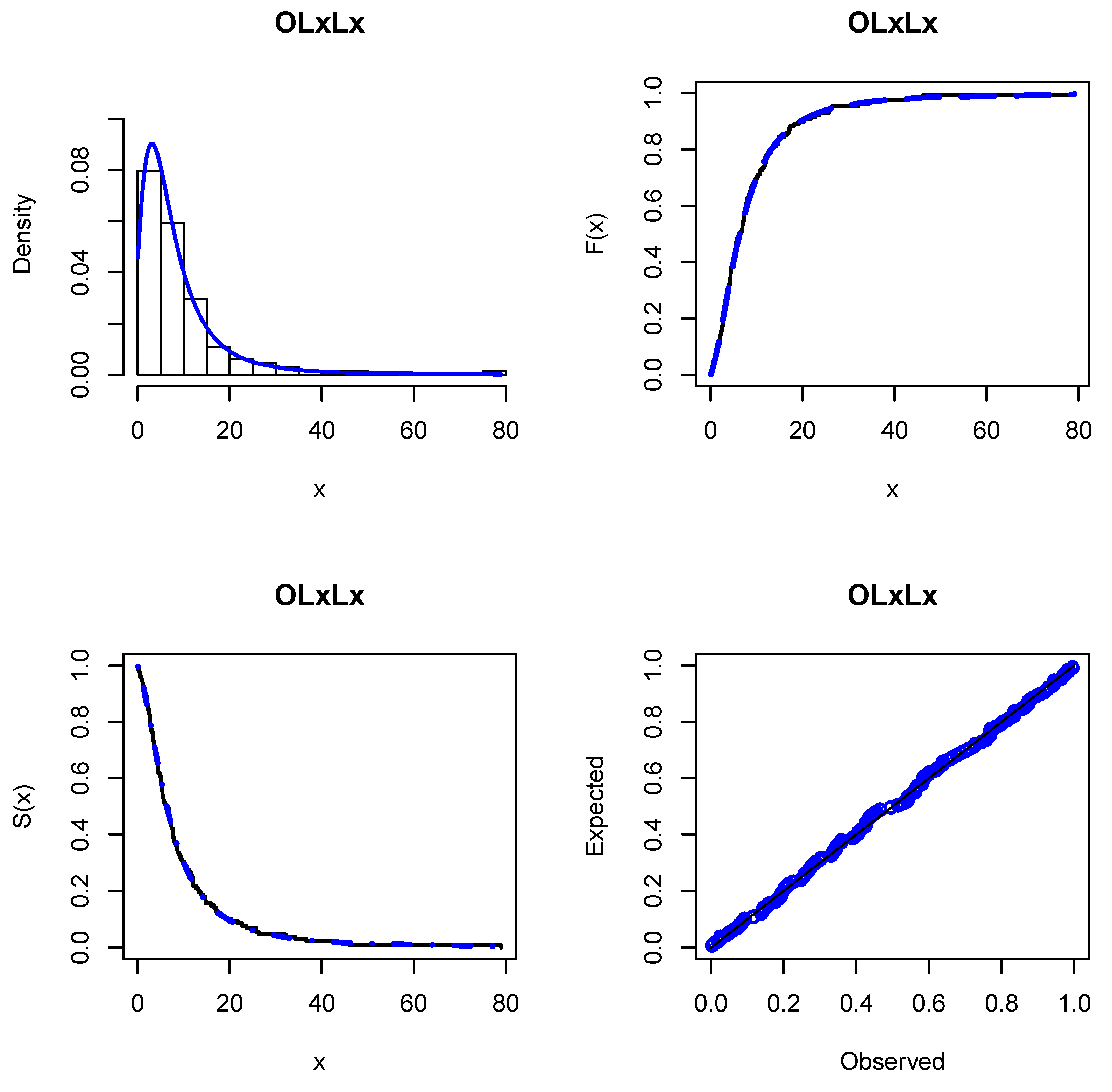
The relative histogram of cancer data with the fitted functions of the OLxLx model, including the fitted PDF, CDF, SF, and (probability-probability) P-P plots, are given in Figure 3. The plots in this figure support and confirm the results in Table 10. Hence, the OLxLx distribution can be used more effectively to model bladder cancer data compared to other competing Lx extensions.
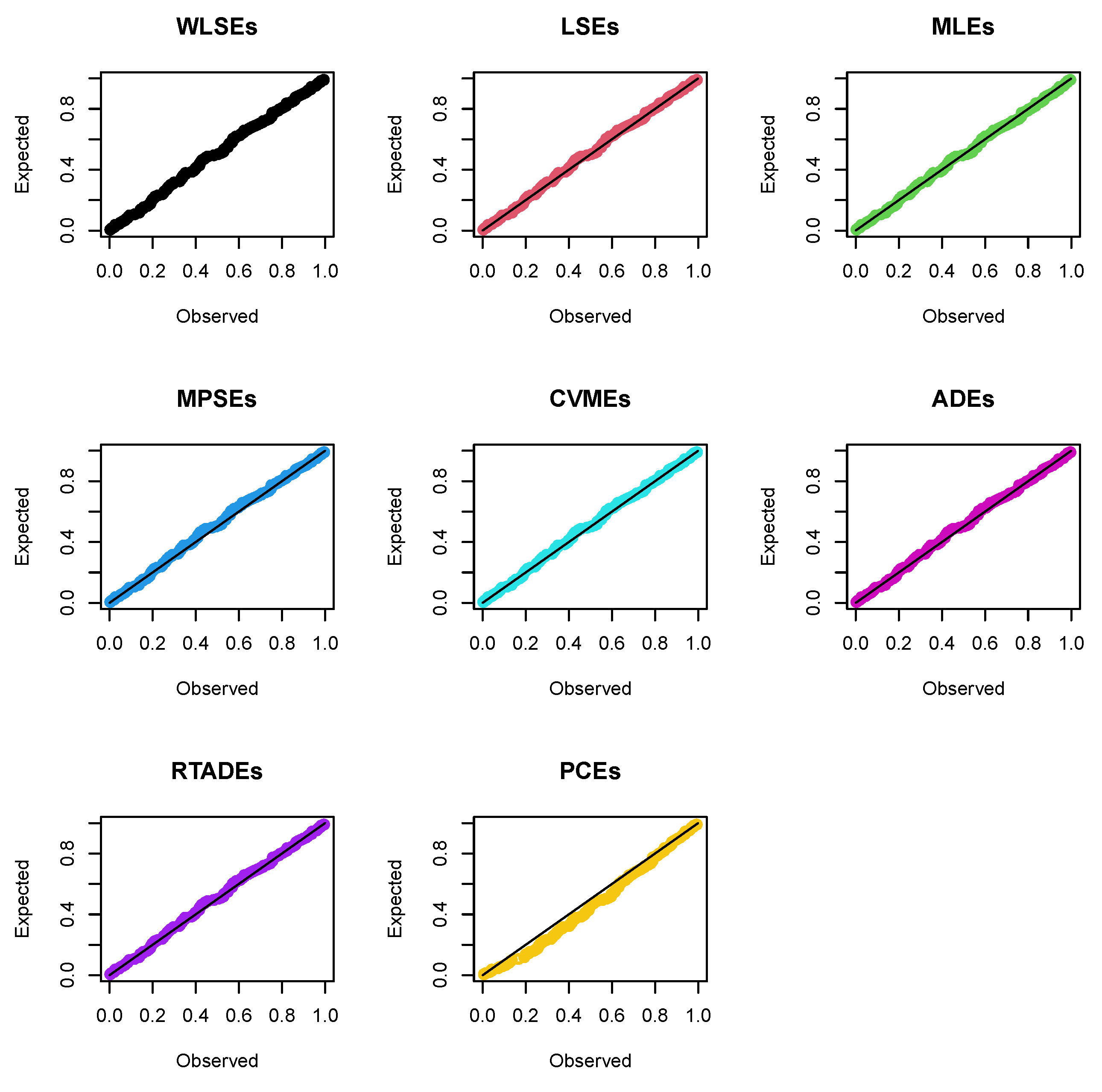
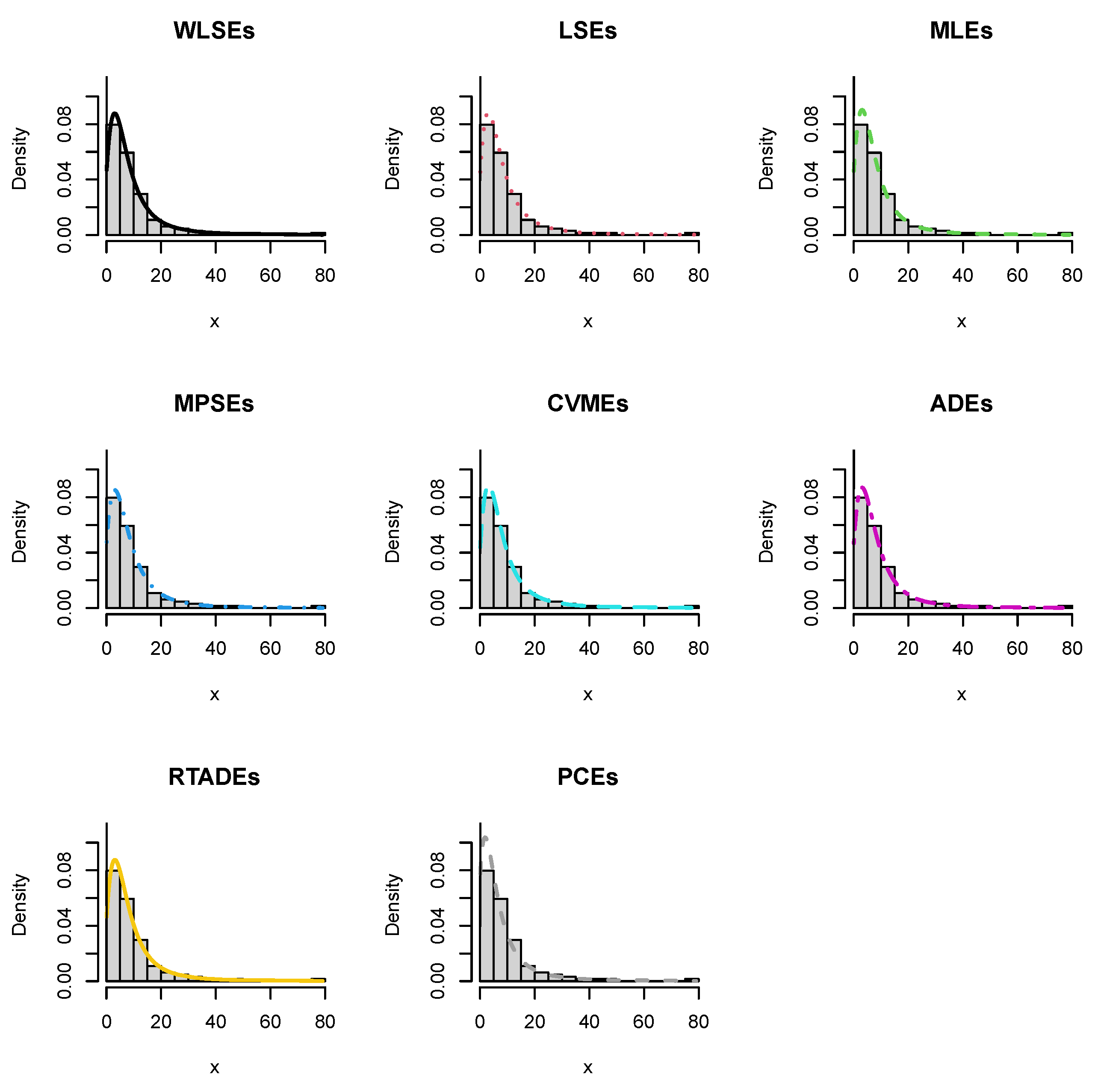
Table 11 shows the parameter estimates of the OLXLX model, KS, and KS p-values under several estimation methods for cancer data. From Table 11, and based on the KS p-values, all estimation methods, except the PCEs, are recommended for estimating the OLxLx parameters for cancer data. Additionally, Figure 4 and Figure 5 display the probability–probability (PP) plots and histograms along with fitted OLxLx density under various estimation methods for bladder cancer data. The plots support the results in Table 11 visually.
7. Conclusions
In this article, a new three-parameter extension of the Lomax distribution, called the odd Lomax–Lomax (OLxLx) distribution, is studied. The hazard function of the OLxLx distribution provides constant, increasing, decreasing, and unimodal shapes. Its density provides symmetrical, right-skewed, left-skewed, and J shaped densities. The parameters of the OLxLx distribution are estimated by eight estimation methods. A detailed simulation study is presented showing that maximum product of spacings has the best performance in estimating the OLxLx parameters. A real-life data from the medical field is fitted using the OLxLx distribution and other fourteen competing models. The real-life application shows the flexibility and superiority of the OLxLx distribution in fitting the analyzed data.
The work of this paper can be extended in light of skew-elliptical distributions following the works of Azzalini and Valle [28], Branco and Dey [29], Loperfido [30], and Adcock et al. [31]. Furthermore, the estimation of the model parameters can be addressed using the Bayesian approach under complete and censored samples. Additionally, quantile regression model by exploiting the flexibility of the OLxLx distribution can be constructed.
Funding
This research was funded by the Deanship of Scientific Research at Qassim University.
Data Availability Statement
This work is mainly a methodological development and has been applied on secondary data; however, if required, data will be provided.
Acknowledgments
The researcher would like to thank the Deanship of Scientific Research, Qassim University, for funding the publication of this project.
Conflicts of Interest
The author declares no conflict of interest.
References
- Atkinson, M.; Harrison, A.J. Personal Wealth in Britan; CUP Archive: Cambridge, UK, 1978. [Google Scholar]
- Corbellini, A.; Crosato, L.; Ganugi, P.; Mazzoli, M. Fitting Pareto II distributions on firm size: Statistical methodology and economic puzzles. In Advances in Data Analysis: Theory and Applications to Reliability and Inference, Data Mining, Bioinformatics, Lifetime Data, and Neural Networks; Springer: Berlin/Heidelberg, Germany, 2010; pp. 321–328. [Google Scholar]
- Harris, C.M. The Pareto distribution as a queue service discipline. Oper. Res. 1968, 16, 307–313. [Google Scholar] [CrossRef]
- Hassan, A.S.; Al-Ghamdi, A.S. Optimum step stress accelerated life testing for Lomax distribution. J. Appl. Sci. Res. 2009, 5, 2153–2164. [Google Scholar]
- Chahkandi, M.; Ganjali, M. On some lifetime distributions with decreasing failure rate. Comput. Stat. Data Anal. 2009, 53, 4433–4440. [Google Scholar] [CrossRef]
- Arnold, B.C. Pareto Distributions; International Cooperative Publishing House: Fairland, MD, USA, 1983. [Google Scholar]
- Johnson, N.L.; Kotz, S.; Balakrishnan, N. Contineous Univariate Distributions, 2nd ed.; Wiley: New York, NY, USA, 1994; Volume 1. [Google Scholar]
- Tahir, M.H.; Cordeiro, G.M.; Mansoor, M.; Zubair, M. The Weibull-Lomax distribution: Properties and applications. Hacet. J. Math. Stat. 2015, 44, 461–480. [Google Scholar] [CrossRef]
- Gupta, R.C.; Gupta, P.L.; Gupta, R.D. Modeling failure time data by Lehman alternatives. Commun. Stat.—Theory Methods 1998, 27, 887–904. [Google Scholar] [CrossRef]
- Ghitany, M.E.; AL-Awadhi, F.A.; Alkhalfan, L.A. Marshall-Olkin extended Lomax distribution and its applications to censored data. Commun. Stat.—Theory Methods 2007, 36, 1855–1866. [Google Scholar] [CrossRef]
- Lemonte, A.J.; Cordeiro, G.M. An extended Lomax distribution. Statistics 2013, 47, 800–816. [Google Scholar] [CrossRef]
- Afify, A.Z.; Yousof, H.M.; Nadarajah, S. The beta transmuted-H family for lifetime data. Stat. Its Interface 2017, 10, 505–520. [Google Scholar] [CrossRef] [Green Version]
- Reyad, H.; Korkmaz, M.Ç.; Afify, A.Z.; Hamedani, G.G.; Othman, S. The Fréchet Topp Leone-G Family of Distributions: Properties, Characterizations and Applications. Ann. Data Sci. 2021, 8, 345–366. [Google Scholar] [CrossRef]
- Afify, A.Z.; Marzouk, W.; Al-Mofleh, H.; Ahmed, A.H.N.; Abdel-Fatah, N.A. The extended failure rate family: Properties and applications in the engineering and insurance fields. Pak. J. Stat. 2022, 38, 165–196. [Google Scholar]
- Cordeiro, G.M.; Afify, A.Z.; Ortega, E.M.M.; Suzuki, A.K.; Mead, M.E. The odd Lomax generator of distributions: Properties, estimation and applications. J. Comput. Appl. Math. 2019, 347, 222–237. [Google Scholar] [CrossRef]
- Marshall, A.W.; Olkin, I. A new method for adding a parameter to a family of distributions with application to the exponential and Weibull families. Biometrika 1997, 84, 641–652. [Google Scholar] [CrossRef]
- Kao, J.H.K. Computer methods for estimating Weibull parameters in reliability studies. IRE Trans. Reliab. Qual. Control 1958, PGRQC-13, 15–22. [Google Scholar] [CrossRef]
- Kao, J.H.K. A graphical estimation of mixed Weibull parameters in life-testing of electron tubes. Technometrics 1959, 1, 389–407. [Google Scholar] [CrossRef]
- Lee, E.T.; Wang, J. Statistical Methods for Survival Data Analysis, 3rd ed.; John Wiley & Sons, Inc.: Hoboken, NJ, USA, 2003. [Google Scholar]
- Alizadeh, M.; Yousof, H.M.; Afify, A.Z.; Cordeiro, G.M.; Mansoor, M. The complementary generalized transmuted Poisson-G family of distributions. Austrian J. Stat. 2018, 47, 60–80. [Google Scholar] [CrossRef] [Green Version]
- Cordeiro, G.M.; Ortega, E.M.M.; Popović, B.V.; Pescim, R.R. The Lomax generator of distributions: Properties, minification process and regression model. Appl. Math. Comput. 2014, 247, 465–486. [Google Scholar] [CrossRef]
- Afify, A.Z.; Nofal, Z.M.; Yousof, H.M.; El Gebaly, Y.M.; Butt, N.S. The transmuted Weibull Lomax distribution: Properties and application. Pak. J. Stat. Oper. Res. 2015, 11, 135–152. [Google Scholar] [CrossRef] [Green Version]
- Mead, M.E. On five-parameter Lomax distribution: Properties and applications. Pak. J. Stat. Oper. Res. 2016, 185–199. [Google Scholar] [CrossRef]
- Alsubie, A. Properties and Applications of the Modified Kies–Lomax Distribution with Estimation Methods. J. Math. 2021, 2021, 1944864. [Google Scholar] [CrossRef]
- Yousof, H.M.; Afify, A.Z.; Hamedani, G.G.; Aryal, G.R. The Burr X Generator of Distributions for Lifetime Data. J. Stat. Theory Appl. 2017, 16, 288–305. [Google Scholar] [CrossRef] [Green Version]
- Afify, A.Z.; Altun, E.; Alizadeh, M.; Ozel, G.; Hamedani, G.G. The odd exponentiated half-logistic-G family: Properties, characterizations and applications. Chil. J. Stat. 2017, 8, 65–91. [Google Scholar]
- Ashour, S.K.; Eltehiwy, M.A. Transmuted Lomax distribution. Am. J. Appl. Math. Stat. 2013, 1, 121–127. [Google Scholar] [CrossRef] [Green Version]
- Azzalini, A.; Valle, A.D. The multivariate skew-normal distribution. Biometrika 1996, 83, 715–726. [Google Scholar] [CrossRef]
- Branco, M.D.; Dey, D.K. A general class of skew-elliptical distributions. J. Multivar. Anal. 2001, 79, 99–113. [Google Scholar] [CrossRef] [Green Version]
- Loperfido, N. A note on skew-elliptical distributions and linear functions of order statistics. Stat. Probab. Lett. 2008, 78, 3184–3186. [Google Scholar] [CrossRef] [Green Version]
- Adcock, C.; Eling, M.; Loperfido, N. Skewed distributions in finance and actuarial science: A review. Eur. J. Financ. 2015, 21, 1253–1281. [Google Scholar] [CrossRef]
Figure 1.
Possible PDF curves of the OLxLx distribution for several parametric values.

Figure 2.
Possible HRF curves of the OLxLx distribution for several parametric values.

Figure 3.
Plots of different fitted functions of the OLxLx distribution for bladder cancer data.

Figure 4.
The PP plots of the OLxLx distribution under various methods for bladder cancer data.

Figure 5.
The histogram for bladder cancer data of the OLxLx distribution under various methods.


Table 1.
Simulation results of the OLxLx distribution for .
| n | Est. | Est. Par. | MLEs | LSEs | WLSEs | CVMEs | MPSEs | PCEs | ADEs | RADEs |
|---|---|---|---|---|---|---|---|---|---|---|
| 20 | |BIAS| | 0.43143 | 0.50890 | 0.45418 | 0.50575 | 0.42194 | 1.14419 | 0.38930 | 0.38625 | |
| 0.16811 | 0.22023 | 0.21715 | 0.21717 | 0.23105 | 0.32886 | 0.19369 | 0.19767 | |||
| 0.43118 | 0.44652 | 0.44074 | 0.42916 | 0.45088 | 0.46119 | 0.41615 | 0.41456 | |||
| MSE | 0.48740 | 0.90300 | 0.64177 | 0.79482 | 0.44170 | 7.06738 | 0.43607 | 0.40702 | ||
| 0.06393 | 0.11739 | 0.11187 | 0.14413 | 0.11451 | 0.54764 | 0.07457 | 0.10771 | |||
| 0.33375 | 0.33738 | 0.32119 | 0.33373 | 0.32510 | 0.31242 | 0.28809 | 0.27864 | |||
| MRE | 0.95873 | 1.13089 | 1.00930 | 1.12388 | 0.93764 | 2.54263 | 0.86511 | 0.85833 | ||
| 0.48032 | 0.62923 | 0.62043 | 0.62049 | 0.66015 | 0.93960 | 0.55341 | 0.56477 | |||
| 0.57490 | 0.59536 | 0.58765 | 0.57221 | 0.60118 | 0.61492 | 0.55487 | 0.55274 | |||
| 30 | 59 | 41 | 47 | 47 | 67 | 18 | 15 | |||
| 50 | 0.24922 | 0.30069 | 0.27029 | 0.28416 | 0.24979 | 0.46826 | 0.24049 | 0.23431 | ||
| |BIAS| | 0.13839 | 0.16465 | 0.16884 | 0.15607 | 0.19783 | 0.22878 | 0.15976 | 0.16480 | ||
| 0.30610 | 0.34174 | 0.33185 | 0.32444 | 0.32865 | 0.36275 | 0.31743 | 0.31700 | |||
| 0.11764 | 0.21149 | 0.15814 | 0.19123 | 0.10876 | 0.74438 | 0.11731 | 0.10023 | |||
| MSE | 0.04000 | 0.05259 | 0.05696 | 0.04891 | 0.07823 | 0.07836 | 0.04875 | 0.04690 | ||
| 0.15046 | 0.17574 | 0.16500 | 0.15967 | 0.15601 | 0.17832 | 0.15186 | 0.14091 | |||
| 0.55383 | 0.66820 | 0.60064 | 0.63147 | 0.55510 | 1.04059 | 0.53441 | 0.52068 | |||
| MRE | 0.39539 | 0.47043 | 0.48239 | 0.44592 | 0.56523 | 0.65365 | 0.45646 | 0.47086 | ||
| 0.40814 | 0.45565 | 0.44247 | 0.43258 | 0.43820 | 0.48367 | 0.42324 | 0.42266 | |||
| 17 | 55 | 51 | 39 | 45 | 72 | 25 | 20 | |||
| 80 | 0.20012 | 0.23963 | 0.20857 | 0.23990 | 0.20504 | 0.31514 | 0.19291 | 0.19882 | ||
| |BIAS| | 0.13054 | 0.14640 | 0.14307 | 0.14271 | 0.18082 | 0.21396 | 0.13863 | 0.15053 | ||
| 0.26096 | 0.29772 | 0.27839 | 0.28953 | 0.28327 | 0.31801 | 0.26596 | 0.27666 | |||
| 0.07122 | 0.11386 | 0.08207 | 0.12124 | 0.06509 | 0.22388 | 0.06488 | 0.06421 | |||
| MSE | 0.03683 | 0.04178 | 0.04247 | 0.03994 | 0.06692 | 0.06676 | 0.03850 | 0.04205 | ||
| 0.10839 | 0.12880 | 0.11396 | 0.12433 | 0.11453 | 0.13487 | 0.10288 | 0.10711 | |||
| 0.44471 | 0.53251 | 0.46348 | 0.53311 | 0.45564 | 0.70030 | 0.42868 | 0.44182 | |||
| MRE | 0.37298 | 0.41830 | 0.40877 | 0.40773 | 0.51663 | 0.61130 | 0.39609 | 0.43008 | ||
| 0.34795 | 0.39697 | 0.37119 | 0.38604 | 0.37769 | 0.42401 | 0.35461 | 0.36888 | |||
| 18 | 53 | 41 | 48 | 48 | 71 | 15 | 30 | |||
| 150 | 0.16273 | 0.19231 | 0.16351 | 0.18302 | 0.15429 | 0.23966 | 0.15803 | 0.15529 | ||
| |BIAS| | 0.11087 | 0.13220 | 0.11867 | 0.12187 | 0.14822 | 0.19296 | 0.11979 | 0.12714 | ||
| 0.21620 | 0.25102 | 0.22574 | 0.23872 | 0.22446 | 0.27365 | 0.22272 | 0.22311 | |||
| 0.04671 | 0.06282 | 0.04419 | 0.05780 | 0.03618 | 0.10279 | 0.04005 | 0.03675 | |||
| MSE | 0.02807 | 0.03685 | 0.03090 | 0.03039 | 0.05099 | 0.05963 | 0.03119 | 0.03472 | ||
| 0.07960 | 0.08897 | 0.07454 | 0.08172 | 0.07718 | 0.10248 | 0.07238 | 0.07240 | |||
| 0.36162 | 0.42736 | 0.36336 | 0.40670 | 0.34287 | 0.53259 | 0.35117 | 0.34509 | |||
| MRE | 0.31677 | 0.37771 | 0.33907 | 0.34820 | 0.42348 | 0.55130 | 0.34224 | 0.36326 | ||
| 0.28826 | 0.33469 | 0.30098 | 0.31829 | 0.29929 | 0.36486 | 0.29696 | 0.29748 | |||
| 23 | 60 | 34 | 46 | 36 | 72 | 24 | 29 | |||
| 500 | 0.11344 | 0.11794 | 0.09984 | 0.11716 | 0.08691 | 0.14311 | 0.09587 | 0.09661 | ||
| |BIAS| | 0.08020 | 0.08307 | 0.07528 | 0.08213 | 0.07615 | 0.13761 | 0.07372 | 0.07424 | ||
| 0.15325 | 0.15940 | 0.14296 | 0.15871 | 0.12712 | 0.18755 | 0.13843 | 0.13831 | |||
| 0.03127 | 0.02143 | 0.01592 | 0.02116 | 0.01346 | 0.03133 | 0.01503 | 0.01467 | |||
| MSE | 0.01839 | 0.01664 | 0.01471 | 0.01620 | 0.01797 | 0.04030 | 0.01486 | 0.01435 | ||
| 0.05617 | 0.03919 | 0.03289 | 0.03844 | 0.03085 | 0.05619 | 0.03213 | 0.03129 | |||
| 0.25208 | 0.26209 | 0.22187 | 0.26035 | 0.19312 | 0.31803 | 0.21305 | 0.21470 | |||
| MRE | 0.22914 | 0.23734 | 0.21510 | 0.23466 | 0.21757 | 0.39317 | 0.21062 | 0.21212 | ||
| 0.20434 | 0.21253 | 0.19062 | 0.21161 | 0.16949 | 0.25006 | 0.18457 | 0.18442 | |||
| 51 | 59 | 32 | 50 | 20 | 72 | 21 | 19 |
Table 2.
Simulation results of the OLxLx distribution for .
| n | Est. | Est. Par. | MLEs | LSEs | WLSEs | CVMEs | MPSEs | PCEs | ADEs | RADEs |
|---|---|---|---|---|---|---|---|---|---|---|
| 20 | |BIAS| | 0.21949 | 0.19925 | 0.19179 | 0.21102 | 0.16233 | 0.18503 | 0.19534 | 0.20818 | |
| 2.09115 | 1.97412 | 1.74062 | 2.14426 | 1.64389 | 1.56467 | 1.47604 | 1.90650 | |||
| 1.29950 | 1.10917 | 1.07834 | 1.23157 | 0.90590 | 0.96122 | 1.06118 | 1.16826 | |||
| MSE | 0.06780 | 0.08081 | 0.06732 | 0.07986 | 0.03580 | 0.09352 | 0.07208 | 0.08746 | ||
| 12.16351 | 11.36830 | 9.17222 | 13.40949 | 9.00936 | 7.10955 | 6.58475 | 12.68988 | |||
| 2.60241 | 2.34379 | 2.16066 | 2.83554 | 1.22953 | 1.46427 | 1.84796 | 2.51992 | |||
| MRE | 0.48776 | 0.44278 | 0.42620 | 0.46894 | 0.36073 | 0.41118 | 0.43409 | 0.46262 | ||
| 1.67292 | 1.57930 | 1.39250 | 1.71541 | 1.31511 | 1.25174 | 1.18083 | 1.52520 | |||
| 1.03960 | 0.88733 | 0.86267 | 0.98526 | 0.72472 | 0.76897 | 0.84894 | 0.93460 | |||
| 62 | 48 | 32 | 65 | 15 | 24 | 24 | 54 | |||
| 50 | 0.18161 | 0.17412 | 0.16664 | 0.17867 | 0.13817 | 0.16364 | 0.16208 | 0.18797 | ||
| |BIAS| | 0.92482 | 1.05999 | 0.84781 | 1.11104 | 0.70657 | 0.77302 | 0.75802 | 0.91179 | ||
| 0.99912 | 0.94217 | 0.90300 | 0.99165 | 0.74384 | 0.84587 | 0.87275 | 0.99883 | |||
| 0.05049 | 0.04355 | 0.04846 | 0.04641 | 0.02871 | 0.04557 | 0.03809 | 0.06756 | |||
| MSE | 2.20945 | 3.15930 | 1.81270 | 3.46078 | 1.38539 | 1.43871 | 1.32728 | 2.31052 | ||
| 1.49793 | 1.26478 | 1.22443 | 1.49444 | 0.85984 | 1.03484 | 1.12340 | 1.53687 | |||
| 0.40359 | 0.38694 | 0.37031 | 0.39703 | 0.30704 | 0.36365 | 0.36018 | 0.41771 | |||
| MRE | 0.73986 | 0.84799 | 0.67825 | 0.88883 | 0.56526 | 0.61842 | 0.60642 | 0.72944 | ||
| 0.79930 | 0.75373 | 0.72240 | 0.79332 | 0.59508 | 0.67670 | 0.69820 | 0.79907 | |||
| 61 | 49 | 38 | 59 | 10 | 25 | 20 | 62 | |||
| 80 | 0.16341 | 0.15965 | 0.14775 | 0.16089 | 0.12364 | 0.15516 | 0.14996 | 0.16752 | ||
| |BIAS| | 0.64810 | 0.82504 | 0.65653 | 0.84366 | 0.50865 | 0.59025 | 0.60458 | 0.66922 | ||
| 0.88765 | 0.86424 | 0.80193 | 0.87459 | 0.65107 | 0.81125 | 0.80479 | 0.89089 | |||
| 0.04447 | 0.03609 | 0.03294 | 0.03948 | 0.02554 | 0.03859 | 0.03375 | 0.04752 | |||
| MSE | 0.86206 | 1.69600 | 0.93102 | 1.77778 | 0.56451 | 0.67174 | 0.70256 | 0.98616 | ||
| 1.27346 | 1.04974 | 0.95637 | 1.09232 | 0.71614 | 0.97790 | 0.96516 | 1.22160 | |||
| 0.36314 | 0.35478 | 0.32833 | 0.35753 | 0.27476 | 0.34481 | 0.33324 | 0.37227 | |||
| MRE | 0.51848 | 0.66003 | 0.52522 | 0.67493 | 0.40692 | 0.47220 | 0.48366 | 0.53537 | ||
| 0.71012 | 0.69139 | 0.64154 | 0.69967 | 0.52085 | 0.64900 | 0.64383 | 0.71271 | |||
| 55 | 50 | 27 | 60 | 9 | 31 | 27 | 65 | |||
| 150 | 0.13588 | 0.13885 | 0.12818 | 0.14479 | 0.10243 | 0.13578 | 0.12883 | 0.14377 | ||
| |BIAS| | 0.45347 | 0.58543 | 0.47960 | 0.59179 | 0.36740 | 0.44209 | 0.45952 | 0.49967 | ||
| 0.72562 | 0.75145 | 0.68986 | 0.78845 | 0.53838 | 0.71491 | 0.68771 | 0.77618 | |||
| 0.03436 | 0.02852 | 0.02634 | 0.03154 | 0.01997 | 0.02941 | 0.02705 | 0.03465 | |||
| MSE | 0.32956 | 0.64980 | 0.38309 | 0.66539 | 0.25686 | 0.30722 | 0.34073 | 0.40687 | ||
| 0.93536 | 0.81780 | 0.74193 | 0.90770 | 0.55021 | 0.79826 | 0.74809 | 0.96131 | |||
| 0.30196 | 0.30857 | 0.28484 | 0.32177 | 0.22762 | 0.30172 | 0.28628 | 0.31950 | |||
| MRE | 0.36277 | 0.46835 | 0.38368 | 0.47343 | 0.29392 | 0.35367 | 0.36762 | 0.39973 | ||
| 0.58049 | 0.60116 | 0.55189 | 0.63076 | 0.43071 | 0.57193 | 0.55017 | 0.62094 | |||
| 43 | 54 | 29 | 68 | 9 | 31 | 28 | 62 | |||
| 500 | 0.08456 | 0.10033 | 0.08575 | 0.10465 | 0.05337 | 0.09235 | 0.08526 | 0.09916 | ||
| |BIAS| | 0.25224 | 0.34542 | 0.27767 | 0.34530 | 0.17300 | 0.27022 | 0.27780 | 0.31236 | ||
| 0.44718 | 0.54785 | 0.46267 | 0.56902 | 0.27597 | 0.49613 | 0.46033 | 0.54337 | |||
| 0.01854 | 0.01787 | 0.01480 | 0.01940 | 0.00822 | 0.01722 | 0.01453 | 0.01863 | |||
| MSE | 0.10120 | 0.18080 | 0.11915 | 0.17940 | 0.06804 | 0.11007 | 0.11800 | 0.14716 | ||
| 0.47263 | 0.50966 | 0.41210 | 0.54875 | 0.22827 | 0.47478 | 0.40250 | 0.53834 | |||
| 0.18790 | 0.22295 | 0.19055 | 0.23256 | 0.11861 | 0.20522 | 0.18947 | 0.22035 | |||
| MRE | 0.20179 | 0.27633 | 0.22214 | 0.27624 | 0.13840 | 0.21617 | 0.22224 | 0.24989 | ||
| 0.35774 | 0.43828 | 0.37014 | 0.45521 | 0.22078 | 0.39690 | 0.36827 | 0.43470 | |||
| 24 | 63 | 35 | 69 | 9 | 38 | 30 | 56 |
Table 3.
Simulation results of the OLxLx distribution for .
| n | Est. | Est. Par. | MLEs | LSEs | WLSEs | CVMEs | MPSEs | PCEs | ADEs | RADEs |
|---|---|---|---|---|---|---|---|---|---|---|
| 20 | |BIAS| | 0.23131 | 0.19347 | 0.18824 | 0.22044 | 0.16818 | 0.17595 | 0.20078 | 0.20678 | |
| 1.81723 | 1.70582 | 1.46058 | 1.81229 | 1.44213 | 1.64385 | 1.31400 | 1.74351 | |||
| 0.76512 | 0.60703 | 0.59499 | 0.69872 | 0.54571 | 0.55394 | 0.62013 | 0.65619 | |||
| MSE | 0.08605 | 0.05951 | 0.05349 | 0.08083 | 0.04142 | 0.05206 | 0.06219 | 0.09781 | ||
| 7.14691 | 6.94228 | 5.20980 | 7.97822 | 5.33075 | 6.92205 | 4.22640 | 8.75147 | |||
| 0.88641 | 0.55017 | 0.52287 | 0.80224 | 0.43406 | 0.44311 | 0.58111 | 0.73213 | |||
| MRE | 0.51403 | 0.42993 | 0.41831 | 0.48988 | 0.37374 | 0.39100 | 0.44617 | 0.45951 | ||
| 1.45379 | 1.36466 | 1.16846 | 1.44983 | 1.15371 | 1.31508 | 1.05120 | 1.39481 | |||
| 1.02016 | 0.80937 | 0.79332 | 0.93163 | 0.72762 | 0.73858 | 0.82684 | 0.87492 | |||
| 69 | 39 | 26 | 62 | 13 | 24 | 33 | 58 | |||
| 50 | 0.20336 | 0.17387 | 0.16611 | 0.18323 | 0.14716 | 0.15965 | 0.16669 | 0.17399 | ||
| |BIAS| | 0.91965 | 1.08478 | 0.87526 | 1.13228 | 0.74843 | 0.86259 | 0.76077 | 0.88666 | ||
| 0.62457 | 0.53928 | 0.51687 | 0.58090 | 0.45684 | 0.49977 | 0.50851 | 0.53975 | |||
| 0.07056 | 0.04380 | 0.04168 | 0.05042 | 0.03576 | 0.03446 | 0.04381 | 0.05071 | |||
| MSE | 1.73599 | 2.84070 | 1.74071 | 3.07360 | 1.33295 | 1.96437 | 1.23641 | 2.02244 | ||
| 0.61996 | 0.39510 | 0.38074 | 0.46786 | 0.33254 | 0.34245 | 0.38451 | 0.42983 | |||
| 0.45192 | 0.38637 | 0.36913 | 0.40718 | 0.32702 | 0.35477 | 0.37042 | 0.38665 | |||
| MRE | 0.73572 | 0.86782 | 0.70021 | 0.90582 | 0.59874 | 0.69007 | 0.60862 | 0.70933 | ||
| 0.83276 | 0.71905 | 0.68916 | 0.77453 | 0.60912 | 0.66636 | 0.67802 | 0.71967 | |||
| 63 | 50 | 32 | 65 | 11 | 22 | 28 | 53 | |||
| 80 | 0.17526 | 0.15990 | 0.15312 | 0.16485 | 0.13028 | 0.15080 | 0.15235 | 0.15787 | ||
| |BIAS| | 0.68462 | 0.83446 | 0.69720 | 0.83998 | 0.53486 | 0.64435 | 0.61539 | 0.67009 | ||
| 0.53124 | 0.49960 | 0.47421 | 0.51831 | 0.39954 | 0.46878 | 0.46279 | 0.48684 | |||
| 0.05866 | 0.03826 | 0.03752 | 0.04160 | 0.03042 | 0.03207 | 0.03841 | 0.03945 | |||
| MSE | 0.89397 | 1.56642 | 1.04020 | 1.58796 | 0.59038 | 0.86476 | 0.71468 | 1.00968 | ||
| 0.49576 | 0.34945 | 0.33879 | 0.38039 | 0.27410 | 0.30581 | 0.33056 | 0.34608 | |||
| 0.38947 | 0.35533 | 0.34027 | 0.36634 | 0.28950 | 0.33512 | 0.33856 | 0.35082 | |||
| MRE | 0.54770 | 0.66757 | 0.55776 | 0.67199 | 0.42789 | 0.51548 | 0.49232 | 0.53607 | ||
| 0.70833 | 0.66614 | 0.63228 | 0.69108 | 0.53272 | 0.62504 | 0.61705 | 0.64912 | |||
| 62 | 55 | 41 | 66 | 9 | 23 | 24 | 44 | |||
| 150 | 0.15124 | 0.14042 | 0.13267 | 0.14267 | 0.11206 | 0.13651 | 0.13449 | 0.13228 | ||
| |BIAS| | 0.47732 | 0.60202 | 0.50525 | 0.59714 | 0.38293 | 0.46043 | 0.46029 | 0.49195 | ||
| 0.45132 | 0.44019 | 0.40865 | 0.44673 | 0.33799 | 0.42368 | 0.40870 | 0.41391 | |||
| 0.04902 | 0.03189 | 0.03116 | 0.03371 | 0.02628 | 0.02882 | 0.03259 | 0.02804 | |||
| MSE | 0.37974 | 0.70390 | 0.45079 | 0.70633 | 0.27144 | 0.34252 | 0.34810 | 0.40653 | ||
| 0.39695 | 0.29003 | 0.27268 | 0.30653 | 0.22430 | 0.26986 | 0.27967 | 0.26222 | |||
| 0.33610 | 0.31205 | 0.29483 | 0.31705 | 0.24903 | 0.30337 | 0.29886 | 0.29395 | |||
| MRE | 0.38185 | 0.48161 | 0.40420 | 0.47771 | 0.30634 | 0.36834 | 0.36823 | 0.39356 | ||
| 0.60176 | 0.58691 | 0.54487 | 0.59564 | 0.45066 | 0.56490 | 0.54493 | 0.55188 | |||
| 60 | 58 | 36 | 64 | 9 | 34 | 32 | 31 | |||
| 500 | 0.08437 | 0.09794 | 0.08291 | 0.09950 | 0.06040 | 0.09353 | 0.08118 | 0.09108 | ||
| |BIAS| | 0.25668 | 0.34439 | 0.28098 | 0.34214 | 0.19507 | 0.28700 | 0.26743 | 0.29363 | ||
| 0.25392 | 0.31025 | 0.25828 | 0.31555 | 0.18344 | 0.29413 | 0.25194 | 0.28723 | |||
| 0.02140 | 0.01919 | 0.01567 | 0.01993 | 0.00991 | 0.01663 | 0.01546 | 0.01597 | |||
| MSE | 0.10848 | 0.18653 | 0.12608 | 0.18316 | 0.07553 | 0.12370 | 0.11417 | 0.13194 | ||
| 0.17186 | 0.17618 | 0.13883 | 0.18449 | 0.08770 | 0.15746 | 0.13607 | 0.15036 | |||
| 0.18748 | 0.21764 | 0.18424 | 0.22111 | 0.13422 | 0.20785 | 0.18040 | 0.20239 | |||
| MRE | 0.20534 | 0.27551 | 0.22479 | 0.27371 | 0.15605 | 0.22960 | 0.21395 | 0.23491 | ||
| 0.33856 | 0.41367 | 0.34437 | 0.42074 | 0.24459 | 0.39218 | 0.33592 | 0.38297 | |||
| 34 | 65 | 33 | 68 | 9 | 48 | 21 | 46 |
Table 4.
Simulation results of the OLxLx distribution for .
| n | Est. | Est. Par. | MLEs | LSEs | WLSEs | CVMEs | MPSEs | PCEs | ADEs | RADEs |
|---|---|---|---|---|---|---|---|---|---|---|
| 20 | |BIAS| | 0.23968 | 0.23147 | 0.22102 | 0.24444 | 0.17893 | 0.20942 | 0.21395 | 0.25818 | |
| 2.91735 | 3.28627 | 2.74133 | 3.39951 | 2.62260 | 2.54481 | 2.41761 | 3.26759 | |||
| 1.45806 | 1.66848 | 1.51042 | 1.82930 | 1.16339 | 1.25652 | 1.47694 | 1.94695 | |||
| MSE | 0.12823 | 0.14443 | 0.14332 | 0.14974 | 0.10791 | 0.19768 | 0.14236 | 0.19134 | ||
| 20.87416 | 24.51158 | 17.47100 | 26.70102 | 17.54837 | 14.06944 | 13.88508 | 28.76561 | |||
| 7.28694 | 10.45758 | 7.61466 | 10.59888 | 3.93918 | 4.97696 | 7.07777 | 12.39200 | |||
| MRE | 0.53262 | 0.51438 | 0.49115 | 0.54320 | 0.39763 | 0.46537 | 0.47544 | 0.57374 | ||
| 1.16694 | 1.31451 | 1.09653 | 1.35981 | 1.04904 | 1.01792 | 0.96704 | 1.30704 | |||
| 1.94408 | 2.22463 | 2.01389 | 2.43906 | 1.55119 | 1.67536 | 1.96926 | 2.59593 | |||
| 39 | 53 | 38 | 64 | 16 | 24 | 23 | 67 | |||
| 50 | 0.16705 | 0.15814 | 0.13978 | 0.16373 | 0.10665 | 0.11584 | 0.12648 | 0.16772 | ||
| |BIAS| | 1.30738 | 1.91965 | 1.49445 | 1.97249 | 1.29091 | 1.33338 | 1.35028 | 1.56424 | ||
| 0.74298 | 1.07521 | 0.91501 | 1.12159 | 0.67854 | 0.73584 | 0.82934 | 1.17632 | |||
| 0.06862 | 0.07277 | 0.06800 | 0.07772 | 0.03328 | 0.04708 | 0.04802 | 0.09340 | |||
| MSE | 4.09243 | 8.49402 | 4.95803 | 9.18748 | 4.07534 | 3.77715 | 3.86803 | 6.17941 | ||
| 1.92597 | 3.53331 | 2.81227 | 3.88463 | 1.42982 | 1.85209 | 2.21586 | 4.81919 | |||
| 0.37122 | 0.35142 | 0.31063 | 0.36385 | 0.23701 | 0.25742 | 0.28107 | 0.37270 | |||
| MRE | 0.52295 | 0.76786 | 0.59778 | 0.78900 | 0.51637 | 0.53335 | 0.54011 | 0.62570 | ||
| 0.99064 | 1.43362 | 1.22001 | 1.49546 | 0.90472 | 0.98112 | 1.10579 | 1.56842 | |||
| 36 | 55 | 42 | 64 | 11 | 19 | 31 | 66 | |||
| 80 | 0.13526 | 0.12115 | 0.09503 | 0.12680 | 0.07186 | 0.08149 | 0.09389 | 0.12401 | ||
| |BIAS| | 0.93572 | 1.39353 | 1.09376 | 1.46736 | 0.83871 | 0.94471 | 0.98484 | 1.15441 | ||
| 0.51086 | 0.80630 | 0.62649 | 0.85715 | 0.45598 | 0.51701 | 0.61257 | 0.84097 | |||
| 0.04921 | 0.04683 | 0.03177 | 0.04956 | 0.01573 | 0.02220 | 0.02939 | 0.06172 | |||
| MSE | 1.98654 | 4.29261 | 2.51870 | 4.90159 | 1.49529 | 1.78467 | 1.82646 | 2.93187 | ||
| 0.89594 | 2.15718 | 1.38144 | 2.31932 | 0.67688 | 0.90584 | 1.29609 | 2.79171 | |||
| 0.30058 | 0.26922 | 0.21118 | 0.28179 | 0.15969 | 0.18109 | 0.20865 | 0.27557 | |||
| MRE | 0.37429 | 0.55741 | 0.43750 | 0.58695 | 0.33548 | 0.37788 | 0.39394 | 0.46176 | ||
| 0.68114 | 1.07507 | 0.83532 | 1.14287 | 0.60797 | 0.68935 | 0.81676 | 1.12130 | |||
| 36 | 54 | 42 | 68 | 9 | 23 | 32 | 60 | |||
| 150 | 0.10901 | 0.07948 | 0.05681 | 0.07720 | 0.04561 | 0.04971 | 0.05503 | 0.07192 | ||
| |BIAS| | 0.61630 | 0.95944 | 0.73640 | 0.97608 | 0.56206 | 0.63122 | 0.68043 | 0.75896 | ||
| 0.31885 | 0.53323 | 0.37083 | 0.51832 | 0.28853 | 0.31577 | 0.35870 | 0.48517 | |||
| 0.03620 | 0.02271 | 0.01019 | 0.01957 | 0.00555 | 0.00686 | 0.00901 | 0.01852 | |||
| MSE | 0.69440 | 1.84387 | 1.00571 | 1.89282 | 0.60456 | 0.69777 | 0.81534 | 1.02964 | ||
| 0.24442 | 1.01467 | 0.45326 | 0.88502 | 0.23513 | 0.28800 | 0.40393 | 0.88843 | |||
| 0.24225 | 0.17662 | 0.12625 | 0.17155 | 0.10136 | 0.11047 | 0.12228 | 0.15983 | |||
| MRE | 0.24652 | 0.38378 | 0.29456 | 0.39043 | 0.22482 | 0.25249 | 0.27217 | 0.30358 | ||
| 0.42513 | 0.71097 | 0.49443 | 0.69110 | 0.38470 | 0.42103 | 0.47826 | 0.64690 | |||
| 38 | 66 | 42 | 62 | 9 | 22 | 33 | 52 | |||
| 500 | 0.09296 | 0.03261 | 0.02553 | 0.03274 | 0.01972 | 0.02302 | 0.02446 | 0.02908 | ||
| |BIAS| | 0.33940 | 0.47663 | 0.37463 | 0.47751 | 0.24731 | 0.32140 | 0.35821 | 0.39312 | ||
| 0.18648 | 0.21740 | 0.16329 | 0.21798 | 0.12073 | 0.14478 | 0.15642 | 0.19021 | |||
| 0.03431 | 0.00237 | 0.00121 | 0.00241 | 0.00076 | 0.00095 | 0.00106 | 0.00173 | |||
| MSE | 0.17417 | 0.37906 | 0.23114 | 0.38001 | 0.13540 | 0.16907 | 0.20571 | 0.25308 | ||
| 0.06637 | 0.10772 | 0.05106 | 0.10957 | 0.03013 | 0.03878 | 0.04416 | 0.07921 | |||
| 0.20659 | 0.07248 | 0.05672 | 0.07275 | 0.04382 | 0.05115 | 0.05436 | 0.06462 | |||
| MRE | 0.13576 | 0.19065 | 0.14985 | 0.19100 | 0.09893 | 0.12856 | 0.14328 | 0.15725 | ||
| 0.24864 | 0.28986 | 0.21771 | 0.29065 | 0.16097 | 0.19304 | 0.20856 | 0.25362 | |||
| 48 | 60 | 39 | 69 | 9 | 18 | 30 | 51 |
Table 5.
Simulation results of the OLxLx distribution for .
| n | Est. | Est. Par. | MLEs | LSEs | WLSEs | CVMEs | MPSEs | PCEs | ADEs | RADEs |
|---|---|---|---|---|---|---|---|---|---|---|
| 20 | |BIAS| | 0.26440 | 0.27140 | 0.27404 | 0.28624 | 0.21756 | 0.24609 | 0.25505 | 0.29296 | |
| 3.71244 | 4.32795 | 3.28525 | 4.50763 | 2.95481 | 2.73069 | 2.75979 | 3.82620 | |||
| 10.78117 | 9.69086 | 9.57232 | 12.12504 | 6.27003 | 7.24078 | 8.67848 | 11.98645 | |||
| MSE | 0.17705 | 0.15639 | 0.16293 | 0.17487 | 0.11991 | 0.14341 | 0.15146 | 0.17661 | ||
| 52.93173 | 65.36489 | 39.51464 | 71.26457 | 36.51284 | 22.02327 | 27.77793 | 61.75642 | |||
| 495.06002 | 694.26802 | 402.32698 | 999.80169 | 141.10150 | 192.83668 | 283.71288 | 787.63885 | |||
| MRE | 0.58755 | 0.60311 | 0.60898 | 0.63610 | 0.48346 | 0.54687 | 0.56679 | 0.65103 | ||
| 1.48498 | 1.73118 | 1.31410 | 1.80305 | 1.18192 | 1.09228 | 1.10392 | 1.53048 | |||
| 4.31247 | 3.87635 | 3.82893 | 4.85002 | 2.50801 | 2.89631 | 3.47139 | 4.79458 | |||
| 48 | 51 | 41 | 68 | 15 | 15 | 24 | 62 | |||
| 50 | 0.14771 | 0.21454 | 0.18365 | 0.21389 | 0.13210 | 0.15862 | 0.16607 | 0.21055 | ||
| |BIAS| | 1.36063 | 1.92830 | 1.52590 | 2.06722 | 1.18536 | 1.32585 | 1.30724 | 1.58710 | ||
| 4.63894 | 6.39807 | 5.52336 | 6.84825 | 3.63832 | 4.30041 | 4.93046 | 7.04501 | |||
| 0.06982 | 0.11457 | 0.09479 | 0.11565 | 0.05058 | 0.07876 | 0.08433 | 0.11493 | |||
| MSE | 4.91841 | 10.07173 | 5.66180 | 12.86291 | 3.97461 | 3.60574 | 3.71836 | 6.04345 | ||
| 93.50937 | 133.55169 | 109.88900 | 155.23946 | 49.53378 | 69.82118 | 93.84751 | 170.36460 | |||
| 0.32825 | 0.47676 | 0.40811 | 0.47532 | 0.29355 | 0.35249 | 0.36904 | 0.46788 | |||
| MRE | 0.54425 | 0.77132 | 0.61036 | 0.82689 | 0.47415 | 0.53034 | 0.52290 | 0.63484 | ||
| 1.85558 | 2.55923 | 2.20935 | 2.73930 | 1.45533 | 1.72016 | 1.97218 | 2.81800 | |||
| 27 | 61 | 45 | 67 | 11 | 22 | 30 | 61 | |||
| 80 | 0.10736 | 0.17533 | 0.13566 | 0.17409 | 0.09045 | 0.11837 | 0.12209 | 0.16353 | ||
| |BIAS| | 0.93766 | 1.34715 | 1.11537 | 1.42250 | 0.82833 | 0.95822 | 0.96822 | 1.16783 | ||
| 3.08584 | 5.12435 | 3.95277 | 5.25137 | 2.38867 | 3.19872 | 3.48486 | 5.18981 | |||
| 0.04925 | 0.08678 | 0.05990 | 0.08664 | 0.02617 | 0.05108 | 0.05196 | 0.07994 | |||
| MSE | 1.69040 | 3.48281 | 2.45678 | 4.36749 | 1.29237 | 1.62218 | 1.65889 | 2.56983 | ||
| 47.37410 | 91.33746 | 65.23730 | 97.89241 | 23.27946 | 44.24889 | 52.08591 | 101.41735 | |||
| 0.23857 | 0.38962 | 0.30146 | 0.38687 | 0.20101 | 0.26305 | 0.27130 | 0.36341 | |||
| MRE | 0.37506 | 0.53886 | 0.44615 | 0.56900 | 0.33133 | 0.38329 | 0.38729 | 0.46713 | ||
| 1.23434 | 2.04974 | 1.58111 | 2.10055 | 0.95547 | 1.27949 | 1.39394 | 2.07592 | |||
| 21 | 63 | 45 | 68 | 9 | 25 | 35 | 58 | |||
| 150 | 0.06372 | 0.12053 | 0.08563 | 0.11880 | 0.05138 | 0.06648 | 0.07851 | 0.10481 | ||
| |BIAS| | 0.63776 | 0.98124 | 0.77219 | 0.96167 | 0.53420 | 0.65510 | 0.71271 | 0.81705 | ||
| 1.70773 | 3.41183 | 2.31767 | 3.42894 | 1.29135 | 1.71092 | 2.13844 | 3.13376 | |||
| 0.01571 | 0.04865 | 0.02657 | 0.04830 | 0.00898 | 0.01606 | 0.02321 | 0.03890 | |||
| MSE | 0.70234 | 1.69995 | 0.99417 | 1.62977 | 0.56126 | 0.72199 | 0.85644 | 1.12625 | ||
| 14.13687 | 47.08032 | 24.08381 | 49.03672 | 7.61965 | 13.55833 | 21.23868 | 43.27343 | |||
| 0.14159 | 0.26784 | 0.19029 | 0.26399 | 0.11419 | 0.14773 | 0.17446 | 0.23292 | |||
| MRE | 0.25510 | 0.39250 | 0.30888 | 0.38467 | 0.21368 | 0.26204 | 0.28508 | 0.32682 | ||
| 0.68309 | 1.36473 | 0.92707 | 1.37158 | 0.51654 | 0.68437 | 0.85538 | 1.25350 | |||
| 19 | 69 | 45 | 66 | 9 | 26 | 36 | 54 | |||
| 500 | 0.02611 | 0.04740 | 0.03164 | 0.04637 | 0.01577 | 0.02615 | 0.03087 | 0.03989 | ||
| |BIAS| | 0.31961 | 0.51418 | 0.38211 | 0.50490 | 0.20047 | 0.32053 | 0.37145 | 0.43745 | ||
| 0.62810 | 1.22797 | 0.77588 | 1.19235 | 0.34998 | 0.62185 | 0.75559 | 1.04335 | |||
| 0.00126 | 0.00681 | 0.00200 | 0.00651 | 0.00091 | 0.00121 | 0.00186 | 0.00419 | |||
| MSE | 0.16168 | 0.43448 | 0.23739 | 0.42697 | 0.11103 | 0.16197 | 0.22183 | 0.31511 | ||
| 0.80855 | 5.85144 | 1.37521 | 5.31883 | 0.57506 | 0.73520 | 1.25554 | 3.78249 | |||
| 0.05803 | 0.10534 | 0.07030 | 0.10304 | 0.03505 | 0.05812 | 0.06860 | 0.08865 | |||
| MRE | 0.12784 | 0.20567 | 0.15284 | 0.20196 | 0.08019 | 0.12821 | 0.14858 | 0.17498 | ||
| 0.25124 | 0.49119 | 0.31035 | 0.47694 | 0.13999 | 0.24874 | 0.30223 | 0.41734 | |||
| 22 | 72 | 45 | 63 | 9 | 23 | 36 | 54 |
Table 6.
Simulation results of the OLxLx distribution for .
| n | Est. | Est. Par. | MLEs | LSEs | WLSEs | CVMEs | MPSEs | PCEs | ADEs | RADEs |
|---|---|---|---|---|---|---|---|---|---|---|
| 20 | |BIAS| | 0.23878 | 0.24396 | 0.24627 | 0.26625 | 0.20949 | 0.21562 | 0.21892 | 0.27273 | |
| 3.26900 | 3.78271 | 3.12508 | 3.96325 | 2.94905 | 2.63540 | 2.62525 | 3.40534 | |||
| 3.17062 | 3.30235 | 3.25808 | 4.08908 | 2.46608 | 2.49712 | 2.88089 | 4.11162 | |||
| MSE | 0.14494 | 0.13885 | 0.15604 | 0.15729 | 0.20220 | 0.14180 | 0.13783 | 0.16791 | ||
| 31.52626 | 39.33780 | 28.02026 | 45.05061 | 27.73351 | 17.33411 | 20.61758 | 38.53511 | |||
| 35.86071 | 42.53578 | 38.15151 | 75.54361 | 25.62682 | 20.55147 | 29.72342 | 58.14463 | |||
| MRE | 0.53063 | 0.54214 | 0.54727 | 0.59167 | 0.46553 | 0.47915 | 0.48649 | 0.60608 | ||
| 1.30760 | 1.51308 | 1.25003 | 1.58530 | 1.17962 | 1.05416 | 1.05010 | 1.36214 | |||
| 2.53650 | 2.64188 | 2.60647 | 3.27127 | 1.97286 | 1.99769 | 2.30471 | 3.28929 | |||
| 39 | 51 | 44 | 66 | 23 | 17 | 20 | 64 | |||
| 50 | 0.14636 | 0.18289 | 0.15546 | 0.18599 | 0.11457 | 0.13984 | 0.13544 | 0.18408 | ||
| |BIAS| | 1.40142 | 1.91400 | 1.49214 | 2.01377 | 1.22101 | 1.27504 | 1.32233 | 1.52051 | ||
| 1.54273 | 2.24324 | 1.92478 | 2.45685 | 1.33734 | 1.56097 | 1.67967 | 2.46450 | |||
| 0.07482 | 0.08933 | 0.08058 | 0.09458 | 0.03882 | 0.08081 | 0.06196 | 0.09814 | |||
| MSE | 5.24588 | 9.16209 | 5.50591 | 11.09046 | 3.87622 | 3.44698 | 3.98643 | 5.69719 | ||
| 9.61286 | 15.48749 | 13.75485 | 19.90902 | 6.22504 | 9.33753 | 10.79651 | 20.73653 | |||
| 0.32526 | 0.40641 | 0.34546 | 0.41330 | 0.25461 | 0.31075 | 0.30098 | 0.40907 | |||
| MRE | 0.56057 | 0.76560 | 0.59686 | 0.80551 | 0.48840 | 0.51002 | 0.52893 | 0.60820 | ||
| 1.23418 | 1.79459 | 1.53982 | 1.96548 | 1.06987 | 1.24878 | 1.34373 | 1.97160 | |||
| 30 | 57 | 44 | 68 | 10 | 24 | 27 | 64 | |||
| 80 | 0.11286 | 0.14127 | 0.11133 | 0.14524 | 0.07938 | 0.09739 | 0.09775 | 0.14033 | ||
| |BIAS| | 0.93519 | 1.38362 | 1.08576 | 1.41838 | 0.83483 | 0.94620 | 0.95028 | 1.09694 | ||
| 1.00720 | 1.72331 | 1.34372 | 1.80902 | 0.91205 | 1.11050 | 1.17674 | 1.82842 | |||
| 0.03957 | 0.06172 | 0.04451 | 0.06508 | 0.01989 | 0.04105 | 0.03414 | 0.06562 | |||
| MSE | 1.99894 | 4.37866 | 2.42338 | 4.65549 | 1.46965 | 1.71354 | 1.67412 | 2.30403 | ||
| 4.14404 | 10.30272 | 7.14115 | 11.27000 | 3.02250 | 5.25501 | 5.48062 | 12.92332 | |||
| 0.25081 | 0.31394 | 0.24740 | 0.32276 | 0.17641 | 0.21641 | 0.21723 | 0.31184 | |||
| MRE | 0.37408 | 0.55345 | 0.43431 | 0.56735 | 0.33393 | 0.37848 | 0.38011 | 0.43878 | ||
| 0.80576 | 1.37865 | 1.07498 | 1.44721 | 0.72964 | 0.88840 | 0.94139 | 1.46274 | |||
| 27 | 59 | 44 | 68 | 9 | 26 | 30 | 61 | |||
| 150 | 0.07916 | 0.09234 | 0.06598 | 0.09739 | 0.04744 | 0.05370 | 0.06188 | 0.08371 | ||
| |BIAS| | 0.60417 | 0.93455 | 0.71725 | 0.94703 | 0.55438 | 0.62816 | 0.67554 | 0.78638 | ||
| 0.58639 | 1.10967 | 0.77242 | 1.18687 | 0.53433 | 0.60694 | 0.72470 | 1.04052 | |||
| 0.02172 | 0.03049 | 0.01572 | 0.03319 | 0.00646 | 0.01076 | 0.01303 | 0.02561 | |||
| MSE | 0.63314 | 1.69239 | 0.90962 | 1.69186 | 0.59297 | 0.68376 | 0.77597 | 1.10317 | ||
| 1.17626 | 4.85779 | 2.47806 | 5.43586 | 0.95156 | 1.50187 | 1.98384 | 4.50230 | |||
| 0.17592 | 0.20520 | 0.14662 | 0.21642 | 0.10542 | 0.11933 | 0.13751 | 0.18603 | |||
| MRE | 0.24167 | 0.37382 | 0.28690 | 0.37881 | 0.22175 | 0.25126 | 0.27022 | 0.31455 | ||
| 0.46911 | 0.88773 | 0.61793 | 0.94949 | 0.42746 | 0.48555 | 0.57976 | 0.83241 | |||
| 27 | 64 | 42 | 71 | 9 | 24 | 33 | 54 | |||
| 500 | 0.05679 | 0.03777 | 0.02722 | 0.03579 | 0.01914 | 0.02327 | 0.02636 | 0.03366 | ||
| |BIAS| | 0.32101 | 0.48260 | 0.37000 | 0.47775 | 0.23830 | 0.31328 | 0.35561 | 0.41255 | ||
| 0.26678 | 0.43749 | 0.30681 | 0.41468 | 0.20536 | 0.25571 | 0.29599 | 0.39159 | |||
| 0.01701 | 0.00347 | 0.00139 | 0.00293 | 0.00080 | 0.00094 | 0.00126 | 0.00243 | |||
| MSE | 0.15952 | 0.37621 | 0.22276 | 0.37201 | 0.12676 | 0.15874 | 0.20217 | 0.27346 | ||
| 0.12177 | 0.51414 | 0.18753 | 0.42653 | 0.09799 | 0.11775 | 0.16554 | 0.36393 | |||
| 0.12620 | 0.08394 | 0.06048 | 0.07954 | 0.04254 | 0.05171 | 0.05858 | 0.07479 | |||
| MRE | 0.12840 | 0.19304 | 0.14800 | 0.19110 | 0.09532 | 0.12531 | 0.14224 | 0.16502 | ||
| 0.21342 | 0.35000 | 0.24545 | 0.33175 | 0.16429 | 0.20457 | 0.23679 | 0.31327 | |||
| 42 | 69 | 42 | 60 | 9 | 18 | 33 | 51 |
Table 7.
Simulation results of the OLxLx distribution for .
| n | Est. | Est. Par. | MLEs | LSEs | WLSEs | CVMEs | MPSEs | PCEs | ADEs | RADEs |
|---|---|---|---|---|---|---|---|---|---|---|
| 20 | |BIAS| | 2.16925 | 2.93594 | 2.66136 | 2.60921 | 2.42171 | 5.47792 | 2.38732 | 2.50875 | |
| 0.18321 | 0.21043 | 0.22429 | 0.21662 | 0.21391 | 0.31140 | 0.19373 | 0.21197 | |||
| 0.60782 | 0.67376 | 0.66541 | 0.67088 | 0.63670 | 0.68196 | 0.65902 | 0.66558 | |||
| MSE | 10.85598 | 24.69643 | 18.47048 | 20.01900 | 14.04590 | 159.55140 | 13.76235 | 15.86948 | ||
| 0.09480 | 0.09669 | 0.11056 | 0.14195 | 0.09051 | 0.45840 | 0.06728 | 0.09828 | |||
| 0.60870 | 0.69410 | 0.66142 | 0.71312 | 0.62071 | 0.66654 | 0.68228 | 0.67693 | |||
| MRE | 0.72308 | 0.97865 | 0.88712 | 0.86974 | 0.80724 | 1.82597 | 0.79577 | 0.83625 | ||
| 0.52346 | 0.60124 | 0.64084 | 0.61892 | 0.61116 | 0.88972 | 0.55350 | 0.60564 | |||
| 0.48625 | 0.53901 | 0.53233 | 0.53671 | 0.50936 | 0.54557 | 0.52722 | 0.53246 | |||
| 11 | 52 | 48 | 55 | 27 | 68 | 23 | 40 | |||
| 50 | 1.43580 | 1.72642 | 1.61271 | 1.72443 | 1.49943 | 2.43544 | 1.46905 | 1.55709 | ||
| |BIAS| | 0.15206 | 0.16951 | 0.16564 | 0.16597 | 0.18985 | 0.23094 | 0.16332 | 0.17880 | ||
| 0.45734 | 0.50889 | 0.49411 | 0.51160 | 0.49309 | 0.54503 | 0.48060 | 0.50088 | |||
| 3.69183 | 5.71382 | 4.74933 | 6.00416 | 4.05320 | 15.66070 | 3.64201 | 4.20995 | |||
| MSE | 0.05291 | 0.05025 | 0.05016 | 0.04714 | 0.07438 | 0.10380 | 0.04788 | 0.05407 | ||
| 0.31544 | 0.36158 | 0.34701 | 0.37169 | 0.35066 | 0.39350 | 0.32195 | 0.35031 | |||
| 0.47860 | 0.57547 | 0.53757 | 0.57481 | 0.49981 | 0.81181 | 0.48968 | 0.51903 | |||
| MRE | 0.43447 | 0.48433 | 0.47324 | 0.47421 | 0.54242 | 0.65983 | 0.46664 | 0.51085 | ||
| 0.36587 | 0.40711 | 0.39529 | 0.40928 | 0.39447 | 0.43602 | 0.38448 | 0.40071 | |||
| 14 | 52 | 35 | 49 | 41 | 72 | 17 | 44 | |||
| 80 | 1.15981 | 1.42027 | 1.26742 | 1.41779 | 1.19915 | 1.82079 | 1.22139 | 1.30153 | ||
| |BIAS| | 0.13680 | 0.15057 | 0.14291 | 0.14507 | 0.16722 | 0.20904 | 0.14132 | 0.15617 | ||
| 0.38571 | 0.44556 | 0.42099 | 0.44360 | 0.42296 | 0.48472 | 0.41287 | 0.43161 | |||
| 2.20214 | 3.29629 | 2.56883 | 3.48002 | 2.48390 | 6.35040 | 2.37524 | 2.72452 | |||
| MSE | 0.04546 | 0.04275 | 0.04002 | 0.03971 | 0.06221 | 0.06820 | 0.03963 | 0.04461 | ||
| 0.22545 | 0.27583 | 0.25042 | 0.27846 | 0.26824 | 0.31303 | 0.24099 | 0.26293 | |||
| 0.38660 | 0.47342 | 0.42247 | 0.47260 | 0.39972 | 0.60693 | 0.40713 | 0.43384 | |||
| MRE | 0.39085 | 0.43020 | 0.40831 | 0.41449 | 0.47776 | 0.59727 | 0.40378 | 0.44620 | ||
| 0.30857 | 0.35645 | 0.33679 | 0.35488 | 0.33837 | 0.38778 | 0.33030 | 0.34529 | |||
| 14 | 54 | 30 | 48 | 41 | 72 | 19 | 46 | |||
| 150 | 0.91952 | 1.08389 | 0.96903 | 1.11611 | 0.87261 | 1.34497 | 0.96065 | 1.00373 | ||
| |BIAS| | 0.11404 | 0.12596 | 0.11293 | 0.12288 | 0.13600 | 0.18020 | 0.11614 | 0.13069 | ||
| 0.31682 | 0.35727 | 0.32919 | 0.36643 | 0.33085 | 0.40149 | 0.33237 | 0.34956 | |||
| 1.34756 | 1.80477 | 1.46867 | 1.94623 | 1.41290 | 2.95790 | 1.41340 | 1.52554 | |||
| MSE | 0.03498 | 0.03441 | 0.02859 | 0.03061 | 0.04929 | 0.05550 | 0.02993 | 0.03588 | ||
| 0.15822 | 0.18617 | 0.16318 | 0.19213 | 0.18311 | 0.22968 | 0.16451 | 0.18110 | |||
| 0.30651 | 0.36130 | 0.32301 | 0.37204 | 0.29087 | 0.44832 | 0.32022 | 0.33458 | |||
| MRE | 0.32583 | 0.35989 | 0.32267 | 0.35108 | 0.38858 | 0.51485 | 0.33184 | 0.37341 | ||
| 0.25346 | 0.28581 | 0.26335 | 0.29314 | 0.26468 | 0.32119 | 0.26590 | 0.27965 | |||
| 17 | 50 | 21 | 53 | 36 | 72 | 28 | 47 | |||
| 500 | 0.53401 | 0.66504 | 0.56192 | 0.64836 | 0.37758 | 0.83816 | 0.56954 | 0.57252 | ||
| |BIAS| | 0.06631 | 0.07516 | 0.06322 | 0.07168 | 0.05798 | 0.11978 | 0.06453 | 0.06821 | ||
| 0.19082 | 0.22489 | 0.19470 | 0.22013 | 0.15947 | 0.26919 | 0.19781 | 0.19732 | |||
| 0.48497 | 0.70558 | 0.51350 | 0.65778 | 0.44060 | 1.09130 | 0.51757 | 0.53459 | |||
| MSE | 0.01557 | 0.01503 | 0.01087 | 0.01350 | 0.01530 | 0.03260 | 0.01112 | 0.01319 | ||
| 0.06634 | 0.08493 | 0.06483 | 0.07996 | 0.06322 | 0.12275 | 0.06602 | 0.06826 | |||
| 0.17800 | 0.22168 | 0.18731 | 0.21612 | 0.12586 | 0.27939 | 0.18985 | 0.19084 | |||
| MRE | 0.18945 | 0.21474 | 0.18063 | 0.20479 | 0.16566 | 0.34222 | 0.18438 | 0.19487 | ||
| 0.15266 | 0.17991 | 0.15576 | 0.17611 | 0.12758 | 0.21535 | 0.15825 | 0.15785 | |||
| 29 | 61 | 22 | 52 | 14 | 72 | 33 | 41 |
Table 8.
Simulation results of the OLxLx distribution for .
| n | Est. | Est. Par. | MLEs | LSEs | WLSEs | CVMEs | MPSEs | PCEs | ADEs | RADEs |
|---|---|---|---|---|---|---|---|---|---|---|
| 20 | |BIAS| | 2.48720 | 3.06324 | 2.75433 | 3.00137 | 2.44203 | 7.54395 | 2.37436 | 2.48865 | |
| 0.19124 | 0.22830 | 0.23001 | 0.23692 | 0.22546 | 0.40522 | 0.20611 | 0.20961 | |||
| 0.42225 | 0.44929 | 0.44205 | 0.43128 | 0.42696 | 0.46317 | 0.41740 | 0.43085 | |||
| MSE | 14.62421 | 30.37985 | 20.54163 | 26.32017 | 15.27398 | 301.54150 | 14.38511 | 16.76935 | ||
| 0.10133 | 0.13993 | 0.13388 | 0.18106 | 0.11484 | 0.97360 | 0.09416 | 0.11425 | |||
| 0.31608 | 0.34173 | 0.32763 | 0.33408 | 0.29191 | 0.31728 | 0.29234 | 0.30552 | |||
| MRE | 0.82907 | 1.02108 | 0.91811 | 1.00046 | 0.81401 | 2.51465 | 0.79145 | 0.82955 | ||
| 0.54641 | 0.65227 | 0.65716 | 0.67692 | 0.64419 | 1.15778 | 0.58887 | 0.59888 | |||
| 0.56300 | 0.59905 | 0.58940 | 0.57504 | 0.56927 | 0.61757 | 0.55653 | 0.57446 | |||
| 20 | 59 | 50 | 56 | 26 | 69 | 12 | 32 | |||
| 50 | 1.54547 | 1.91976 | 1.74951 | 1.89441 | 1.46656 | 3.02331 | 1.55242 | 1.54501 | ||
| |BIAS| | 0.13904 | 0.17217 | 0.16781 | 0.16263 | 0.17808 | 0.25633 | 0.15985 | 0.16024 | ||
| 0.29325 | 0.33999 | 0.32841 | 0.33068 | 0.31018 | 0.36505 | 0.31128 | 0.31283 | |||
| 4.78792 | 8.58045 | 6.39022 | 8.41641 | 4.18580 | 28.78420 | 4.75600 | 4.33195 | |||
| MSE | 0.04368 | 0.06186 | 0.05843 | 0.05817 | 0.06416 | 0.20710 | 0.04981 | 0.04489 | ||
| 0.13888 | 0.17521 | 0.16120 | 0.16927 | 0.14429 | 0.17926 | 0.14315 | 0.14036 | |||
| 0.51516 | 0.63992 | 0.58317 | 0.63147 | 0.48885 | 1.00777 | 0.51747 | 0.51500 | |||
| MRE | 0.39725 | 0.49193 | 0.47946 | 0.46467 | 0.50879 | 0.73236 | 0.45673 | 0.45783 | ||
| 0.39100 | 0.45332 | 0.43788 | 0.44090 | 0.41358 | 0.48673 | 0.41504 | 0.41711 | |||
| 16 | 60 | 45 | 48 | 32 | 72 | 27 | 24 | |||
| 80 | 1.23790 | 1.57486 | 1.41474 | 1.56031 | 1.18013 | 2.11711 | 1.31380 | 1.32478 | ||
| |BIAS| | 0.12428 | 0.15053 | 0.14720 | 0.14466 | 0.15719 | 0.22721 | 0.14208 | 0.14914 | ||
| 0.24883 | 0.29575 | 0.28226 | 0.28837 | 0.26380 | 0.32077 | 0.27070 | 0.27489 | |||
| 2.83986 | 5.02446 | 3.71901 | 4.95456 | 2.55790 | 9.79230 | 3.01410 | 2.87589 | |||
| MSE | 0.03804 | 0.04579 | 0.04540 | 0.04411 | 0.05242 | 0.11060 | 0.04037 | 0.04123 | ||
| 0.09823 | 0.12706 | 0.11575 | 0.12213 | 0.10486 | 0.13633 | 0.10589 | 0.10544 | |||
| 0.41263 | 0.52495 | 0.47158 | 0.52010 | 0.39338 | 0.70570 | 0.43793 | 0.44159 | |||
| MRE | 0.35508 | 0.43008 | 0.42057 | 0.41332 | 0.44912 | 0.64916 | 0.40595 | 0.42611 | ||
| 0.33177 | 0.39433 | 0.37635 | 0.38449 | 0.35173 | 0.42769 | 0.36093 | 0.36652 | |||
| 12 | 60 | 43 | 46 | 30 | 72 | 26 | 35 | |||
| 150 | 0.90893 | 1.21687 | 1.09374 | 1.22086 | 0.84860 | 1.55320 | 1.03239 | 1.03274 | ||
| |BIAS| | 0.10555 | 0.12632 | 0.12053 | 0.12220 | 0.12367 | 0.19198 | 0.11983 | 0.12606 | ||
| 0.19238 | 0.24083 | 0.22794 | 0.23816 | 0.20015 | 0.27141 | 0.21894 | 0.22323 | |||
| 1.44104 | 2.50083 | 1.98446 | 2.56440 | 1.42755 | 4.16810 | 1.67202 | 1.63049 | |||
| MSE | 0.03267 | 0.03341 | 0.03258 | 0.03122 | 0.03716 | 0.05960 | 0.03216 | 0.03312 | ||
| 0.05926 | 0.08241 | 0.07624 | 0.08151 | 0.06531 | 0.10141 | 0.07047 | 0.07211 | |||
| 0.30298 | 0.40562 | 0.36458 | 0.40695 | 0.28287 | 0.51773 | 0.34413 | 0.34425 | |||
| MRE | 0.30157 | 0.36093 | 0.34436 | 0.34915 | 0.35335 | 0.54851 | 0.34236 | 0.36019 | ||
| 0.25650 | 0.32111 | 0.30391 | 0.31755 | 0.26686 | 0.36189 | 0.29193 | 0.29765 | |||
| 15 | 59 | 39 | 48 | 26 | 72 | 25 | 40 | |||
| 500 | 0.48952 | 0.78993 | 0.65694 | 0.77312 | 0.32286 | 0.95551 | 0.62809 | 0.64043 | ||
| |BIAS| | 0.06694 | 0.08481 | 0.07377 | 0.08041 | 0.04931 | 0.13680 | 0.07221 | 0.07594 | ||
| 0.11060 | 0.16042 | 0.13999 | 0.15685 | 0.08912 | 0.18694 | 0.13544 | 0.13926 | |||
| 0.45542 | 0.96442 | 0.69129 | 0.92500 | 0.38409 | 1.39480 | 0.64144 | 0.65317 | |||
| MSE | 0.02200 | 0.01755 | 0.01430 | 0.01540 | 0.00992 | 0.03960 | 0.01393 | 0.01546 | ||
| 0.02167 | 0.03958 | 0.03183 | 0.03779 | 0.01981 | 0.05605 | 0.03040 | 0.03208 | |||
| 0.16317 | 0.26331 | 0.21898 | 0.25771 | 0.10762 | 0.31850 | 0.20936 | 0.21348 | |||
| MRE | 0.19124 | 0.24231 | 0.21078 | 0.22973 | 0.14087 | 0.39084 | 0.20632 | 0.21698 | ||
| 0.14747 | 0.21389 | 0.18665 | 0.20914 | 0.11882 | 0.24925 | 0.18059 | 0.18568 | |||
| 23 | 62 | 40 | 52 | 9 | 72 | 26 | 40 |
Table 9.
Partial and overall ranks of different estimation methods of the OLxLx parameters under various parametric values of .
Table 9.
Partial and overall ranks of different estimation methods of the OLxLx parameters under various parametric values of .
| n | MLEs | LSEs | WLSEs | CVMEs | MPSEs | PCEs | ADEs | RADEs | |||
|---|---|---|---|---|---|---|---|---|---|---|---|
| ɵ | |||||||||||
| 0.50 | 0.35 | 0.75 | 20 | 3 | 7 | 4 | 5.5 | 5.5 | 8 | 2 | 1 |
| 50 | 1 | 7 | 6 | 4 | 5 | 8 | 3 | 2 | |||
| 80 | 2 | 7 | 4 | 5.5 | 5.5 | 8 | 1 | 3 | |||
| 150 | 1 | 7 | 4 | 6 | 5 | 8 | 2 | 3 | |||
| 500 | 6 | 7 | 4 | 5 | 2 | 8 | 3 | 1 | |||
| 0.50 | 1.25 | 1.25 | 20 | 7 | 5 | 4 | 8 | 1 | 2.5 | 2.5 | 6 |
| 50 | 7 | 5 | 4 | 6 | 1 | 3 | 2 | 8 | |||
| 80 | 6 | 5 | 2.5 | 7 | 1 | 4 | 2.5 | 8 | |||
| 150 | 5 | 6 | 3 | 8 | 1 | 4 | 2 | 7 | |||
| 500 | 2 | 7 | 4 | 8 | 1 | 5 | 3 | 6 | |||
| 0.75 | 1.25 | 0.75 | 20 | 8 | 5 | 3 | 7 | 1 | 2 | 4 | 6 |
| 50 | 7 | 5 | 4 | 8 | 1 | 2 | 3 | 6 | |||
| 80 | 7 | 6 | 4 | 8 | 1 | 2 | 3 | 5 | |||
| 150 | 7 | 6 | 5 | 8 | 1 | 4 | 3 | 2 | |||
| 500 | 4 | 7 | 3 | 8 | 1 | 6 | 2 | 5 | |||
| 0.75 | 2.25 | 0.75 | 20 | 5 | 6 | 4 | 7 | 1 | 3 | 2 | 8 |
| 50 | 4 | 6 | 5 | 7 | 1 | 2 | 3 | 8 | |||
| 80 | 4 | 6 | 5 | 8 | 1 | 2 | 3 | 7 | |||
| 150 | 4 | 8 | 5 | 7 | 1 | 2 | 3 | 6 | |||
| 500 | 5 | 7 | 4 | 8 | 1 | 2 | 3 | 6 | |||
| 1.5 | 2.25 | 2.5 | 20 | 5 | 6 | 4 | 8 | 1.5 | 1.5 | 3 | 7 |
| 50 | 3 | 6.5 | 5 | 8 | 1 | 2 | 4 | 6.5 | |||
| 80 | 2 | 7 | 5 | 8 | 1 | 3 | 4 | 6 | |||
| 150 | 2 | 8 | 5 | 7 | 1 | 3 | 4 | 6 | |||
| 500 | 2 | 8 | 5 | 7 | 1 | 3 | 4 | 6 | |||
| 1.5 | 2.25 | 1.25 | 20 | 4 | 6 | 5 | 8 | 3 | 1 | 2 | 7 |
| 50 | 4 | 6 | 5 | 8 | 1 | 2 | 3 | 7 | |||
| 80 | 3 | 6 | 5 | 8 | 1 | 2 | 4 | 7 | |||
| 150 | 3 | 7 | 5 | 8 | 1 | 2 | 4 | 6 | |||
| 500 | 4.5 | 8 | 4.5 | 7 | 1 | 2 | 3 | 6 | |||
| 3 | 0.35 | 1.25 | 20 | 1 | 6 | 5 | 7 | 3 | 8 | 2 | 4 |
| 50 | 1 | 7 | 3 | 6 | 4 | 8 | 2 | 5 | |||
| 80 | 1 | 7 | 3 | 6 | 4 | 8 | 2 | 5 | |||
| 150 | 1 | 6 | 2 | 7 | 4 | 8 | 3 | 5 | |||
| 500 | 3 | 7 | 2 | 6 | 1 | 8 | 4 | 5 | |||
| 3 | 0.35 | 0.75 | 20 | 2 | 7 | 5 | 6 | 3 | 8 | 1 | 4 |
| 50 | 1 | 7 | 5 | 6 | 4 | 8 | 3 | 2 | |||
| 80 | 1 | 7 | 5 | 6 | 3 | 8 | 2 | 4 | |||
| 150 | 1 | 7 | 4 | 6 | 3 | 8 | 2 | 5 | |||
| 500 | 2 | 7 | 4.5 | 6 | 1 | 8 | 3 | 4.5 | |||
| 141.5 | 261.5 | 168.5 | 278 | 80.5 | 187 | 111 | 212 | ||||
| Overall Rank | 3 | 7 | 4 | 8 | 1 | 5 | 2 | 6 | |||
Table 10.
The ML estimates, SEs, and fitting measures for bladder cancer data.
| Distribution | Estimates | SEs | AIC | BIC | KS | KS p-Value | |||
|---|---|---|---|---|---|---|---|---|---|
| OLxLx | = 1.854428 | 0.3528995 | 409.5022 | 825.0044 | 833.5605 | 0.015023 | 0.092074 | 0.029928 | 0.999843 |
| = 1.303778 | 0.6083500 | ||||||||
| = 55.746420 | 20.1269541 | ||||||||
| WLx | = 0.072862 | 0.137502 | 410.0418 | 828.0837 | 839.4918 | 0.029264 | 0.194151 | 0.041024 | 0.982411 |
| = 7.312808 | 6.808461 | ||||||||
| = 75.243002 | 247.138134 | ||||||||
| = 1.525593 | 0.284570 | ||||||||
| CGTPLx | = −0.838684 | 0.144250 | 409.6202 | 827.2403 | 838.6484 | 0.018824 | 0.120356 | 0.035205 | 0.997360 |
| = 23.777878 | 106.066481 | ||||||||
| = 0.227014 | 1.364232 | ||||||||
| = 25.997754 | 44.284429 | ||||||||
| LxW | = 2.070040 | 0.968163 | 409.7399 | 827.4798 | 838.8879 | 0.019457 | 0.130771 | 0.035056 | 0.997519 |
| = 12.323896 | 433.967972 | ||||||||
| = 0.482693 | 11.905508 | ||||||||
| = 1.427611 | 0.1779201 | ||||||||
| TWLx | =0.132298 | 0.326495 | 409.8028 | 829.6057 | 843.8658 | 0.023896 | 0.157834 | 0.038419 | 0.991586 |
| = 12.150835 | 15.252054 | ||||||||
| = 0.669019 | 0.452082 | ||||||||
| = 28.320694 | 130.023884 | ||||||||
| =1.462765 | 0.258484 | ||||||||
| ELx | = 1.586198 | 0.279744 | 410.0718 | 826.1436 | 834.6997 | 0.0283230 | 0.190211 | 0.040512 | 0.984604 |
| = 4.585705 | 2.226673 | ||||||||
| = 24.741450 | 16.685800 | ||||||||
| KwLx | = 0.397583 | 2.539788 | 409.9403 | 827.8806 | 839.2887 | 0.025854 | 0.172632 | 0.038924 | 0.990172 |
| = 12.340590 | 18.279746 | ||||||||
| = 1.516220 | 0.266744 | ||||||||
| = 11.801720 | 89.335600 | ||||||||
| MKLx | = 1.612191 | 0.390874 | 410.8951 | 827.7901 | 836.3462 | 0.050520 | 0.325224 | 0.049121 | 0.916932 |
| = 0.392557 | 0.152109 | ||||||||
| = 1.848593 | 1.565668 | ||||||||
| BXLx | = 0.298273 | 0.051134 | 411.1459 | 828.2918 | 836.8479 | 0.054390 | 0.354999 | 0.047712 | 0.932685 |
| = 1.020066 | 0.664080 | ||||||||
| = 0.933832 | 0.249918 | ||||||||
| BELx | =2.021947 | 2.967803 | 409.9135 | 829.8269 | 844.0871 | 0.0254417 | 0.169137 | 0.039074 | 0.989719 |
| = 0.657188 | 2.449987 | ||||||||
| = 0.093312 | 0.123866 | ||||||||
| = 0.744411 | 1.078977 | ||||||||
| = 6.620361 | 29.576475 | ||||||||
| McLx | = 0.808465 | 3.545156 | 409.9125 | 829.8249 | 844.0851 | 0.025352 | 0.168538 | 0.039115 | 0.989595 |
| = 11.292883 | 18.295065 | ||||||||
| = 1.506001 | 0.283714 | ||||||||
| = 4.188648 | 26.365111 | ||||||||
| = 2.104531 | 3.111132 | ||||||||
| OEHLLx | =1.426955 | 0.261373 | 409.728 | 827.456 | 838.8642 | 0.021328 | 0.140743 | 0.036817 | 0.995086 |
| = 26.076262 | 93.761718 | ||||||||
| = 0.106983 | 0.316311 | ||||||||
| = 9.722434 | 8.822504 | ||||||||
| TLx | = 4.020827 | 1.492284 | 409.6258 | 825.2516 | 833.8077 | 0.019549 | 0.125509 | 0.035842 | 0.996591 |
| = 0.052398 | 0.025906 | ||||||||
| = −0.844517 | 0.139368 | ||||||||
| Lx | = 13.93842 | 15.38628 | 413.8329 | 831.6658 | 837.3698 | 0.080679 | 0.487362 | 0.096670 | 0.182695 |
| = 121.02227 | 142.71830 | ||||||||
| TPMOLx | = 2.810465 | 0.227464 | 418.1563 | 840.3125 | 846.0166 | 1.308544 | 7.103445 | 0.199602 | 0.000074 |
| = 179.408493 | 35.185927 |
Table 11.
The OLxLx parameter estimates using several estimation methods along with KS and KS p-value for bladder cancer data.
Table 11.
The OLxLx parameter estimates using several estimation methods along with KS and KS p-value for bladder cancer data.
| Method | KS | KS p-Value | |||
|---|---|---|---|---|---|
| WLSEs | 1.817852 | 1.259341 | 51.54454 | 0.032765 | 0.999396 |
| LSEs | 1.854045 | 1.193350 | 51.61323 | 0.033634 | 0.999052 |
| MLEs | 1.854428 | 1.303778 | 55.746420 | 0.029928 | 0.999843 |
| MPSEs | 1.752837 | 1.470533 | 56.83993 | 0.033684 | 0.999028 |
| CVMEs | 1.876271 | 1.200982 | 54.52999 | 0.0337999 | 0.998971 |
| ADEs | 1.794702 | 1.400382 | 56.83796 | 0.030627 | 0.999832 |
| RADEs | 1.813133 | 1.326467 | 54.75095 | 0.032264 | 0.999542 |
| PCEs | 1.642911 | 1.273914 | 28.02273 | 0.099726 | 0.173070 |
Disclaimer/Publisher’s Note: The statements, opinions and data contained in all publications are solely those of the individual author(s) and contributor(s) and not of MDPI and/or the editor(s). MDPI and/or the editor(s) disclaim responsibility for any injury to people or property resulting from any ideas, methods, instructions or products referred to in the content. |
© 2023 by the author. Licensee MDPI, Basel, Switzerland. This article is an open access article distributed under the terms and conditions of the Creative Commons Attribution (CC BY) license (https://creativecommons.org/licenses/by/4.0/).
Share and Cite
MDPI and ACS Style
Alnssyan, B. The Modified-Lomax Distribution: Properties, Estimation Methods, and Application. Symmetry 2023, 15, 1367. https://doi.org/10.3390/sym15071367
AMA Style
Alnssyan B. The Modified-Lomax Distribution: Properties, Estimation Methods, and Application. Symmetry. 2023; 15(7):1367. https://doi.org/10.3390/sym15071367
Chicago/Turabian StyleAlnssyan, Badr. 2023. "The Modified-Lomax Distribution: Properties, Estimation Methods, and Application" Symmetry 15, no. 7: 1367. https://doi.org/10.3390/sym15071367
Note that from the first issue of 2016, this journal uses article numbers instead of page numbers. See further details here.