Analytical and Numerical Methods for Solving Second-Order Two-Dimensional Symmetric Sequential Fractional Integro-Differential Equations

Abstract

In this paper, we investigate the solution to a class of symmetric non-homogeneous two-dimensional fractional integro-differential equations using both analytical and numerical methods. We first show the differences between the Caputo derivative and the symmetric sequential fractional derivative and how they help facilitate the implementation of numerical and analytical approaches. Then, we propose a numerical approach based on the operational matrix method, which involves deriving operational matrices for the differential and integral terms of the equation and combining them to generate a single algebraic system. This method allows for the efficient and accurate approximation of the solution without the need for projection. Our findings demonstrate the effectiveness of the operational matrix method for solving non-homogeneous fractional integro-differential equations. We then provide examples to test our numerical method. The results demonstrate the accuracy and efficiency of the approach, with the graph of exact and approximate solutions showing almost complete overlap, and the approximate solution to the fractional problem converges to the solution of the integer problem as the order of the fractional derivative approaches one. We use various methods to measure the error in the approximation, such as absolute and $L_2$ errors. Additionally, we explore the effect of the derivative order. The results show that the absolute error is on the order of ${10}^{-14}$, while the $L_2$ error is on the order of ${10}^{-13}$. Next, we apply the Laplace transform to find an analytical solution to a class of fractional integro-differential equations and extend the approach to the two-dimensional case. We consider all homogeneous cases. Through our examples, we achieve two purposes. First, we show how the obtained results are implemented, especially the exact solution for some 1D and 2D classes. We then demonstrate that the exact fractional solution converges to the exact solution of the ordinary derivative as the order of the fractional derivative approaches one.

1. Introduction

Fractional calculus is a branch of mathematical analysis that extends the concepts of differentiation and integration to non-integer orders. The origins of fractional calculus can be traced back to the work of Leibniz and Euler in the 18th century, who introduced the concept of fractional differentiation and integration. However, in the late 19th and early 20th centuries, fractional calculus began to be studied systematically, thanks to the work of mathematicians such as Liouville, Riemann, and Grunwald; see [1]. One of the main results of fractional calculus is the fractional derivative, which is a generalization of the classical derivative to non-integer orders. The fractional derivative has numerous applications in physics, engineering, and other sciences, particularly in problems involving non-locality or memory effects [2].

Another important concept in fractional calculus is the fractional integral, which is a generalization of the classical integral to non-integer orders. The fractional integral is useful for solving differential equations involving fractional derivatives and has applications in areas such as signal processing and control theory.

One of the most significant advancements in the field of fractional calculus is the development of the Caputo fractional derivative. Caputo introduced the fractional derivative in 1967, which is defined as the Riemann–Liouville fractional derivative with the initial conditions being in the form of a non-singular integer. The Caputo fractional derivative is widely used in various applications due to its ability to handle initial conditions better than other types of fractional derivatives; see [2] for more details.

The concept of symmetric sequential fractional derivatives was first introduced by Kilbas, Srivastava, and Trujillo in [3]. They defined the sequential fractional derivative of order $\alpha$ and $\beta ,\alpha ,\beta >0$ as the composition of two fractional derivatives of orders $\alpha$ and $\beta$, respectively. Later, a generalization of this concept was proposed by Zhang and Wei [4], who defined the sequential fractional derivative of arbitrary order as the composition of n fractional derivatives of different orders. In [5], Atanackovic and Pilipovic studied the symmetric sequential fractional derivative in the context of the Caputo sense. They derived the Laplace transform of the symmetric sequential fractional derivative and discussed its basic properties. They also investigated the relationship between the sequential fractional derivative and the fractional integral.

Li et al. [6] introduced a new class of symmetric sequential fractional derivative models and demonstrated their applications in the fields of fluid mechanics, heat transfer, and finance. Zhong et al. [7] discussed the properties of sequential fractional derivatives and their application to fractional partial differential equations. They also showed that the sequential fractional derivative is more general than the Riemann–Liouville fractional derivative.

One of the key properties of symmetric sequential fractional derivatives is their non-commutativity. This means that the order in which the fractional derivatives are applied can affect the final result. This property has been studied in detail by several researchers, such as Baleanu, Gülsuand Mohammadi [8], who have shown that it can have important implications for the behavior of complex systems. Symmetric sequential fractional derivatives have also been used in numerical methods for solving differential equations. Fractional Adams–Bashforth methods that use sequential fractional derivatives to approximate the solution of fractional differential equations have been proposed by Zhang, Li, and Shen [9].

Moreover, different applications in science and engineering are modeled by integro-differential equations (IDEs) and partial differential equations (PDEs); see [10,11]. They arise naturally in many fields, including physics, engineering, economics, and biology. One of the earliest studies of IDEs was performed by Volterra in [12], who developed a theory of integral equations based on his work on functional analysis. Then, the study of IDEs has grown significantly, with many researchers contributing to the development of the field.

On the other hand, in [2], the authors showed one of the key properties of IDEs is their non-locality, which means that the solution at a given point depends not only on the local values of the function but also on its integral over a certain range. This property makes the analysis of IDEs more challenging than that of ordinary differential equations (ODEs).

Several techniques have been developed for solving IDEs, including numerical methods, Laplace transforms, and Fourier transforms. One of the most popular methods for solving IDEs, which has been used by Baleanu et al. [13], is the method of characteristics, which involves finding curves along which the solution to the equation is constant. This method has been applied to a wide range of problems, including those in fluid mechanics, heat transfer, and finance.

The stability analysis of IDEs is another important topic in the study of these equations. Stability analysis involves studying the behavior of the solutions to the IDEs as time passes and determining whether the solutions converge or diverge. Several researchers have developed stability criteria for IDEs, which have been used in the study of problems in biology, finance, and other fields. Wang, Sun, and Li [14] studied the stability of solutions to fractional differential equations with the Caputo derivative. They presented a new sufficient condition for the asymptotic stability of the zero solution to the equation, based on the Lyapunov direct method. In recent years, there has been a growing interest in the use of operational matrices in machine learning and data analysis. Operational matrices can be used to represent data in a low-dimensional space, which can make it easier to analyze and process large datasets. Operational matrices are an important tool in applied mathematics and engineering for solving differential equations and other problems. They are matrices that used to calculate the estimated solution of a differential equation in terms of the values of the function and its derivatives at a finite set of points. Wu and Liao [15] presented an efficient approach to obtain higher-order approximations of fractional derivatives using the generalized Taylor matrix method.

Canuto et al. [16] provided one of the most common methods for solving differential equations using the spectral method. This method involves approximating the solution of a differential equation using a series of orthogonal functions, such as Fourier series or Chebyshev polynomials and then using the corresponding operational matrices to solve for the coefficients of the series. For more detail, we refer the reader to the references [17,18,19,20].

This article is divided into six sections. The first two sections provide a brief overview of the literature on the applications of and solutions to fractional IDEs. We also mention some preliminary definitions and theorems used in this work. More attention is paid to some symmetric sequential derivatives and fractional Laplace transform results. A derivation of the operational matrix method (OMM) can be found in Section 3. A proof of these matrices is given. Section 4 derives exact solutions for 1D and 2D fractional IDEs. All homogeneous cases are considered. Finally, the last two sections provide some examples for two purposes. First, we show how the results obtained are implemented, specifically the exact solution for some IDE classes. Next, we show the efficiency of OMM. In addition, we end the article with some conclusions and concluding remarks.

It is worth mentioning that our investigation focuses on solving a class of symmetric non-homogeneous two-dimensional fractional integro-differential equations using both analytical and numerical methods. Initially, we highlight the distinctions between the Caputo derivative and the symmetric sequential fractional derivative and discuss how these differences aid in the implementation of numerical and analytical approaches. Subsequently, we propose a numerical approach based on the operational matrix method. This approach entails deriving operational matrices for the differential and integral terms of the equation and combining them to form a unified algebraic system. This method enables efficient and precise approximation of the solution without requiring projection.

2. Preliminaries

We start this section by defining two important operators, which are the Caputo fractional derivative and the Riemann–Liouville fractional integral operator.

Definition 1

([3,21]). Let $q,s>0$ and $M\in \mathbb{N}$ with $M-1<q<M$. Then, the Caputo derivative of z(s) of order q is defined as

$${}^c{D}^{q}z\left(s\right)=\frac{1}{\mathsf{\Gamma }(M-q)}{\int }_0^s{(s-r)}^{M-q-1}{z}^{\left(M\right)}\left(r\right)dr$$

(1)

and the fractional integral operator is given by

$$I^{q}z\left(s\right)=\frac{1}{\mathsf{\Gamma }\left(q\right)}{\int }_0^s{(s-r)}^{q-1}z\left(r\right)dr.$$

(2)

The power rule is one of the important rules, and it is given as follows for both operators

$${}^c{D}^q{s}^{\gamma }=\left\{\begin{array}{ccc}0,& & \gamma <q,\gamma \in \left\{0,1,2,...\right\}\\ \frac{\mathsf{\Gamma }(\gamma +1)}{\mathsf{\Gamma }(\gamma -q+1)}{z}^{\gamma -q}& & \mathrm{otherwise}\end{array}\right\}$$

(3)

and

$$I^q{s}^{\gamma }=\frac{\mathsf{\Gamma }(\gamma +1)}{\mathsf{\Gamma }(\gamma +q+1)}{z}^{\gamma +q}.$$

(4)

The relations between these operators are given as follows:

$${}^c{D}^q{I}^{q}z\left(s\right)=z\left(s\right)$$

(5)

and

$$I^q\left({}^c{D}^{q}z\left(x\right)\right)=z\left(x\right)-\sum _{j=0}^{M-1}\frac{z^j\left(0\right)}{j!}{s}^j.$$

(6)

Formula (3) implies that if $\frac{1}{2}<q\le 1$, then

$${}^c{D}^{2q}{s}^q=\frac{\mathsf{\Gamma }(q+1)}{\mathsf{\Gamma }(q-2q+1)}{s}^{q-2q}=\frac{\mathsf{\Gamma }(q+1)}{\mathsf{\Gamma }(1-q)}{s}^{-q}$$

(7)

and

$${}^c{D}^q\left({}^c{D}^q{s}^q\right){=}^c{D}^q\left(\frac{\mathsf{\Gamma }(q+1)}{\mathsf{\Gamma }\left(1\right)}\right)=0.$$

(8)

Thus,

$${}^c{D}^{2q}{s}^q{\ne }^c{D}^q\left({}^c{D}^q{s}^q\right).$$

(9)

Hence, the Caputo derivative is not symmetric-sequential. The definition of a symmetric-sequential derivative is given as follows.

Definition 2

([22,23]). If $q\in (0,1)$ with

$${}^c{D}^{Mq}z\left(s\right)={}^c{D}^q\left({}^c{D}^{(M-1)q}z\left(s\right)\right),M\in \mathbb{N},$$

(10)

then the derivative is called a symmetric-sequential Caputo derivative of order p, which we denote by ${}^{sc}{D}^{Mq}z\left(s\right)$. For simplicity, we use $D^{Mq}z\left(s\right)$ to mean symmetric sequential derivative.

Now, we define a list of interesting functions that we use in this paper.

Definition 3.

Let ${\alpha }_1>0,{\alpha }_2>0$, and $\lambda ,\gamma \in \Re$. Then,

1. 

The one and two Mittag–Leffler functions are

$$E_{{\alpha }_1}\left(s\right)=\sum _{j=0}^{\infty }\frac{s^j}{\mathsf{\Gamma }(j{\alpha }_1+1)},E_{{\alpha }_1,{\alpha }_2}\left(s\right)=\sum _{j=0}^{\infty }\frac{s^j}{\mathsf{\Gamma }(j{\alpha }_1+{\alpha }_2)},$$

(11)

respectively.

2. 

The fractional sine and cosine functions are

$$\begin{array}{ccc}\hfill si{n}_{{\alpha }_1,\lambda ,\gamma }\left(s\right)& =& \frac{E_{{\alpha }_1}\left((\lambda +i\gamma )s\right)-E_{{\alpha }_1}\left((\lambda -i\gamma )s\right)}{2i},\hfill \\ \hfill co{s}_{{\alpha }_1,\lambda ,\gamma }\left(s\right)& =& \frac{E_{{\alpha }_1}\left((\lambda +i\gamma )s\right)+E_{{\alpha }_1}\left((\lambda -i\gamma )s\right)}{2},\hfill \end{array}$$

(12)

respectively.

For the sequential fractional derivative, we mention two important results in the following theorem.

Theorem 1.

Let $q>0$ and $\mathcal{L}\left(r\right(t\left)\right)=R\left(s\right)$. Then, the Laplace transforms $D^{q}r\left(t\right)$ and $D^{2q}r\left(t\right)$ on $[0,\infty )$ are given as

$$\mathcal{L}\left(D^{q}r\left(t\right)\right)=s^{q}R\left(s\right)-s^{q-1}r\left(0\right)$$

(13)

and

$$\mathcal{L}\left(D^{2q}r\left(t\right)\right)=s^{2q}R\left(s\right)-s^{2q-1}r\left(0\right)-s^{q-1}{D}^{q}r\left(0\right).$$

(14)

In the next theorem, we list the Laplace transforms of some functions that we use in this paper.

Theorem 2.

Let $q>0$ and $\alpha \in \Re$. Then, the Laplace transform of Mittag–Leffler and fractional trigonometric functions are given as follows:

$$\begin{array}{ccc}\hfill \mathcal{L}\left(E_q(\pm \alpha t^q)\right)& =& \frac{s^{q-1}}{s^q\mp \alpha },s^q>\alpha ,\hfill \end{array}$$

(15)

$$\begin{array}{ccc}\hfill \mathcal{L}\left(t^q{E}_{q,q}(\pm \alpha t^q)\right)& =& \frac{q{s}^{q-1}}{{(s^q\mp \alpha )}^2},s^q>\alpha ,\hfill \end{array}$$

(16)

$$\begin{array}{ccc}\hfill \mathcal{L}\left({\sin }_{q,\lambda ,\gamma }\left(t^q\right)\right)& =& \frac{\mu s^{q-1}}{{(s^q-\lambda )}^2+{\mu }^2},\hfill \end{array}$$

(17)

$$\begin{array}{ccc}\hfill \mathcal{L}\left({\cos }_{q,\lambda ,\gamma }\left(t^q\right)\right)& =& \frac{s^{q-1}(s^q-\lambda )}{{(s^q-\lambda )}^2+{\mu }^2},\hfill \end{array}$$

(18)

$$\begin{array}{ccc}\hfill \mathcal{L}\left(t^{2q-1}G{E}_q\left(\alpha t^q\right)\right)& =& \frac{1}{{(s^q-\alpha )}^2},\hfill \end{array}$$

(19)

where

$$G{E}_q\left(t\right)=\sum _{j=0}^{\infty }\frac{(j+1)t^j}{\mathsf{\Gamma }\left(q\right(j+2\left)\right)}.$$

(20)

3. Non-Homogeneous Two-Dimensional Fractional Integro-Differential Equations

This section is devoted to the method of solving a class of two-dimensional fractional inegro-differential Equations of the form

$$w_{xx}(x,t)+D_t^{2q}w(x,t)+{\nu }_1{D}_t^{q}w(x,t)+w_x(x,t)+{\nu }_2\left(t\right)w(x,t)+{\nu }_3{I}_t^{q}w(x,t)=g(x,t)$$

(21)

with

$$w(0,t)=w(1,t)=0,t\ge 0$$

(22)

and

$$w(x,0)=r\left(x\right),D_t^{q}w(x,0)=0,0<x<1$$

(23)

on the domain $[0,1]\times [0,\eta ]$, where ${\nu }_1,{\nu }_3$ are real constants, $r\in C^3\left([0,1]\right),{\nu }_2\in C[0,\eta ]$ and $g\in C\left(\right[0,1]\times [0,\eta )$. Before we start the method of solution, we need the following definition.

Definition 4

([24,25,26]). Let $M_1,M_2\in \mathbb{N}$ and ${\mathsf{\Delta }}_x=\frac{1}{M_1}$ and ${\mathsf{\Delta }}_t=\frac{\eta }{M_2}$ be two step sizes in the x and t directions, respectively. Let $x_i=i{\mathsf{\Delta }}_x$ and $t_j=j{\mathsf{\Delta }}_t$ for $i\in A_x=\{0,1,\cdots ,M_1-1\}$ and $j\in A_t=\{0,1,\cdots ,M_2-1\}$. The two-dimensional Block Pulse function (BPF) is a function ${\beta }_{i,j}:[0,1)\times [0,\eta )\to \Re$ defined by

$${\beta }_{i,j}(x,t)=\left\{\begin{array}{c}1,x\in [x_i,x_{i+1}),t\in [t_j,t_{j+1})\hfill \\ 0,\mathit{otherwise}\hfill \end{array}\right.$$

(24)

where $i\in A_x$ and $j\in A_t$.

The two-dimensional BPF can be split into the product of two one-dimensional BPFs as follows.

Theorem 3.

For any $i\in A_x$ and $j\in A_t$, we have

$${\beta }_{i,j}(x,t)={\beta }_{xi}\left(x\right){\beta }_{tj}\left(t\right)$$

(25)

where ${\beta }_{xi}\left(x\right)$ and ${\beta }_{tj}\left(t\right)$ are BPFs on $[0,\eta )$ and $[0,T_{max})$, respectively.

Proof. 

The proof follows directly from the fact that $(x,t)\in [a,b)\times [c,d)$ if and only if $x\in [a,b)$ and $t\in [c,d)$. □

Since $[0,1)\times [t,\eta )$ is divided into disjoint sets $\{[x_i,x_{i+1})\times [t_j,t_{j+1}):i\in A_x,j\in A_t\}$, one can see the following product and orthogonality relations

$$\begin{array}{ccc}\hfill {\beta }_{i_1,j_1}(x,t){\beta }_{i_2,j_2}(x,t)& =& \left\{\begin{array}{cc}{\beta }_{i_1,j_1}(x,t),\hfill & i_1=i_2,j_1=j_2\hfill \\ 0,\hfill & \mathrm{otherwise}\hfill \end{array}\right.,\hfill \end{array}$$

(26)

$$\begin{array}{ccc}\hfill {\int }_0^1{\int }_0^{\eta }{\beta }_{i_1,j_1}(x,t){\beta }_{i_2,j_2}(x,t)dtdx& =& \left\{\begin{array}{cc}{\mathsf{\Delta }}_x{\mathsf{\Delta }}_t,\hfill & i_1=i_2,j_1=j_2\hfill \\ 0,\hfill & \mathrm{otherwise}\hfill \end{array}\right..\hfill \end{array}$$

(27)

Using these two properties, we can prove the completeness property.

Theorem 4.

Let $w\in L^2([0,1)\times [0,\eta ))$ be a bounded function. Then,

$$w(x,t)\approx \sum _{i=0}^{M_1-1}\sum _{j=0}^{M_2-1}{w}_{ij}{\beta }_{i,j}(x,t)$$

(28)

with

$$w_{ij}=\frac{1}{{\mathsf{\Delta }}_x{\mathsf{\Delta }}_t}{\int }_{x_i}^{x_{i+1}}{\int }_{t_j}^{t_{j+1}}w(x,t)dtdx.$$

(29)

Proof. 

After multiplying Equation (28) by ${\beta }_{i,j}(x,t)$ and then integrating both sides, the result of the theorem will follow directly. □

Using Theorem 4, we can approximate the functions $w(x,t),{\nu }_2\left(t\right),g(x,t)$, and $r\left(x\right)$ as

$$\begin{array}{ccc}\hfill w(x,t)& \approx & \sum _{i=0}^{M_1-1}\sum _{j=0}^{M_2-1}{w}_{ij}{\beta }_{xi}\left(x\right){\beta }_{tj}\left(t\right),\hfill \end{array}$$

(30)

$$\begin{array}{ccc}\hfill g(x,t)& \approx & \sum _{i=0}^{M_1-1}\sum _{j=0}^{M_2-1}{g}_{ij}{\beta }_{xi}\left(x\right){\beta }_{tj}\left(t\right),\hfill \end{array}$$

(31)

$$\begin{array}{ccc}\hfill {\nu }_2\left(t\right)& \approx & \sum _{j=0}^{M_2-1}{v}_{2j}{\beta }_{tj}\left(t\right),\hfill \end{array}$$

(32)

$$\begin{array}{ccc}\hfill r\left(x\right)& \approx & \sum _{i=0}^{M_1-1}{r}_i{\beta }_{ix}\left(x\right).\hfill \end{array}$$

(33)

Hence, the sequential derivatives of the function w can be expanded as

$$\begin{array}{ccc}\hfill D_t^{2q}w(x,t)& =& \sum _{i=0}^{M_1-1}\sum _{j=0}^{M_2-1}{w}_{ij}{\beta }_{xi}\left(x\right)D_t^{2q}{\beta }_{tj}\left(t\right),\hfill \end{array}$$

(34)

$$\begin{array}{ccc}\hfill D_t^{q}w(x,t)& =& \sum _{i=0}^{M_1-1}\sum _{j=0}^{M_2-1}{w}_{ij}{\beta }_{xi}\left(x\right)D_t^q{\beta }_{tj}\left(t\right).\hfill \end{array}$$

(35)

In addition, the product and orthogonality relations of BPF imply that

$$\begin{array}{ccc}\hfill {\nu }_2\left(t\right)w(x,t)& =& \left(\sum _{j=0}^{M_2-1}{v}_{2j}{\beta }_{tj}\left(t\right)\right)\left(\sum _{i=0}^{M_1-1}\sum _{j=0}^{M_2-1}{w}_{ij}{\beta }_{xi}\left(x\right){\beta }_{tj}\left(t\right)\right)\hfill \\ & =& \sum _{i=0}^{M_1-1}\sum _{j=0}^{M_2-1}{v}_{2j}{w}_{ij}{\beta }_{xi}\left(x\right){\beta }_{tj}\left(t\right).\hfill \end{array}$$

(36)

If we substitute these approximations in Equation (21), we obtain

$$\begin{array}{ccc}\hfill & & \sum _{i=0}^{M_1-1}\sum _{j=0}^{M_2-1}{w}_{ij}{\beta }_{xi}\left(x\right)D_t^{2q}{\beta }_{tj}\left(t\right)+{\nu }_1\sum _{i=0}^{M_1-1}\sum _{j=0}^{M_2-1}{w}_{ij}{\beta }_{xi}\left(x\right)D_t^q{\beta }_{tj}\left(t\right)\hfill \\ & & +\sum _{i=0}^{M_1-1}\sum _{j=0}^{M_2-1}{v}_{2j}{w}_{ij}{\beta }_{xi}\left(x\right){\beta }_{tj}\left(t\right)+{\nu }_3\sum _{i=0}^{M_1-1}\sum _{j=0}^{M_2-1}{w}_{ij}{\beta }_{xi}\left(x\right)I_t^q{\beta }_{tj}\left(t\right)\hfill \\ & & =\sum _{i=0}^{M_1-1}\sum _{j=0}^{M_2-1}{g}_{i,j}{\beta }_{xi}\left(x\right){\beta }_{tj}\left(t\right)-w_{xx}(x,t)-w_x(x,t).\hfill \end{array}$$

(37)

To be able to write Equation (37) in matrix form, let us define the following matrices:

$${\mathit{\beta }}_{\mathit{x}}=\left(\begin{array}{c}{\beta }_{x0}\left(x\right)\\ {\beta }_{x1}\left(x\right)\\ ⋮\\ {\beta }_{x\left(M_1-1\right)}\left(x\right)\end{array}\right),W=\left(\begin{array}{cccc}{w}_{00}& w_{01}& \cdots & w_{0(M_2-1)}\\ w_{10}& w_{11}& \cdots & w_{1(M_2-1)}\\ ⋮& ⋮& \ddots & ⋮\\ w_{(M_1-1)0}& w_{(M_1-1)1}& \cdots & w_{(M_1-1)(M_2-1)}\end{array}\right),$$

(38)

$${\mathit{\beta }}_{\mathit{t}}=\left(\begin{array}{c}{\beta }_{t0}\left(t\right)\\ {\beta }_{t1}\left(t\right)\\ ⋮\\ {\beta }_{t(M_2-1)}\left(t\right)\end{array}\right),V_2=\left(\begin{array}{cccc}{\nu }_{20}& 0& \cdots & 0\\ 0& {\nu }_{21}& \cdots & 0\\ ⋮& ⋮& \ddots & ⋮\\ 0& 0& \cdots & {\nu }_{2(M_2-1)}\end{array}\right),R=\left(\begin{array}{c}{r}_0\\ r_1\\ ⋮\\ r_{M_1-1}\end{array}\right),$$

(39)

$$\begin{array}{ccc}& & H=\left(\begin{array}{cccc}{g}_{00}& g_{01}& \cdots & g_{0(M_2-1)}\\ g_{10}& g_{11}& \cdots & g_{1(M_2-1)}\\ ⋮& ⋮& \ddots & ⋮\\ g_{(M_1-1)0}& g_{(M_1-1)1}& \cdots & g_{(M_1-1)(M_2-1)}\end{array}\right).\hfill \end{array}$$

(40)

Thus, Equation (37) becomes

$$\begin{array}{ccc}\hfill & & {{\mathit{\beta }}_{\mathit{x}}}^{*}\left(x\right)W{D}_t^{2q}{\mathit{\beta }}_{\mathit{t}}\left(t\right)+{\nu }_1{{\mathit{\beta }}_{\mathit{x}}}^{*}\left(x\right)W{D}_t^q{\mathit{\beta }}_{\mathit{t}}\left(t\right)+{{\mathit{\beta }}_{\mathit{x}}}^{*}\left(x\right)W{V}_2{\mathit{\beta }}_{\mathit{t}}\left(t\right)\hfill \\ & & +{\nu }_3{{\mathit{\beta }}_{\mathit{x}}}^{*}\left(x\right)W{I}_t^q{\mathit{\beta }}_{\mathit{t}}\left(t\right)={{\mathit{\beta }}_{\mathit{x}}}^{*}\left(x\right)G{\mathit{\beta }}_{\mathit{t}}\left(t\right)-w_{xx}(x,t)-w_x(x,t)\hfill \end{array}$$

(41)

where ${}^{*}$ mean the transpose of a matrix. The initial conditions yield to

$$\begin{array}{c}\hfill D_t^{q}w(x,0)=\sum _{i=0}^{M_1-1}\sum _{j=0}^{M_2-1}{w}_{ij}{\beta }_{xi}\left(x\right)D_t^q{\beta }_{tj}\left(0\right)={\mathit{\beta }}_{\mathit{x}}{\left(x\right)}^{*}W{D}_t^q{\mathit{\beta }}_{\mathit{t}}\left(0\right)=0,\end{array}$$

(42)

$$\begin{array}{c}\hfill w(x,0)=\sum _{i=0}^{M_1-1}\sum _{j=0}^{M_2-1}{w}_{ij}{\beta }_{xi}\left(x\right){\beta }_{tj}\left(0\right)={{\mathit{\beta }}_{\mathit{x}}}^{*}\left(x\right)W{\mathit{\beta }}_{\mathit{t}}\left(0\right)={{\mathit{\beta }}_{\mathit{x}}}^{*}R,\end{array}$$

(43)

which give

$$W{D}_t^q{\mathit{\beta }}_{\mathit{t}}\left(0\right)=0$$

(44)

and

$$W{\mathit{\beta }}_{\mathit{t}}\left(0\right)=R.$$

(45)

The next step is to find the operational integration matrix of the Riemann integral.

Theorem 5.

Let

$$I\left(r\left(x\right)\right)={\int }_0^{x}r\left(t\right)dt.$$

(46)

Then, the operational matrix of I is

$$O_I=\frac{{\mathsf{\Delta }}_x}{2}\left(\begin{array}{cccccc}1& 2& 2& \cdots & 2& 2\\ 0& 1& 2& \cdots & 2& 2\\ 0& 0& 1& \ddots & 2& 2\\ ⋮& ⋮& ⋮& \ddots & \ddots & ⋮\\ 0& 0& 0& \cdots & 1& 2\\ 0& 0& 0& \cdots & 0& 1\end{array}\right).$$

(47)

Proof. 

Let $0\le k\le M_1-1$ and $k\in \mathbb{N}$. Then,

$$\begin{array}{ccc}\hfill I\left({\beta }_{xk}\left(x\right)\right)& =& {\int }_0^x{\beta }_{xk}\left(t\right)dt\hfill \end{array}$$

(48)

$$\begin{array}{ccc}& =& \left\{\begin{array}{cc}0,\hfill & x<x_k\hfill \\ x-x_k,\hfill & x_k\le x<x_{k+1}\hfill \\ {\mathsf{\Delta }}_x,\hfill & x_{k+1}\le x<1\hfill \end{array}\right..\hfill \end{array}$$

(49)

Therefore, if

$$I\left({\beta }_{xk}\left(x\right)\right)=\sum _{j=0}^{M_1-1}{\gamma }_{j,k}{\beta }_{xj}\left(x\right),$$

(50)

then

$$\begin{array}{ccc}\hfill {\gamma }_{j,k}& =& \frac{1}{{\mathsf{\Delta }}_x}{\int }_0^1\left(I({\beta }_{xk}\left(t\right)\right){\beta }_{xj}\left(t\right)dt\hfill \end{array}$$

(51)

$$\begin{array}{ccc}& =& \frac{1}{{\mathsf{\Delta }}_x}{\int }_{x_j}^{x_{j+1}}\left(I({\beta }_{xk}\left(t\right)\right)dt\hfill \end{array}$$

(52)

$$\begin{array}{ccc}& =& \left\{\begin{array}{cc}\frac{{\mathsf{\Delta }}_x}{2},\hfill & 0\le j=k\le M_1-1\hfill \\ {\mathsf{\Delta }}_x,\hfill & 0\le j<k\le M_1-1\hfill \\ 0,\hfill & 0\le k<j\le M_1-1\hfill \end{array}\right.\hfill \end{array}$$

(53)

which completes the proof. □

Theorem 5 and Equation (41) give the following equation when we take the Riemann integral

$$\begin{array}{ccc}\hfill & & {{\mathit{\beta }}_{\mathit{x}}}^{*}\left(x\right)O_I^{*}W{D}_t^{2q}{\mathit{\beta }}_{\mathit{t}}\left(t\right)+{\nu }_1{{\mathit{\beta }}_{\mathit{x}}}^{*}\left(x\right)O_I^{*}W{D}_t^q{\mathit{\beta }}_{\mathit{t}}\left(t\right)+{{\mathit{\beta }}_{\mathit{x}}}^{*}\left(x\right)O_I^{*}W{V}_2{\mathit{\beta }}_{\mathit{t}}\left(t\right)\hfill \\ & & +{\nu }_3{{\mathit{\beta }}_{\mathit{x}}}^{*}\left(x\right)O_I^{*}W{I}_t^q{\mathit{\beta }}_{\mathit{t}}\left(t\right)={{\mathit{\beta }}_{\mathit{x}}}^{*}\left(x\right)O_I^{*}G{\mathit{\beta }}_{\mathit{t}}\left(t\right)-w_x(x,t)+w_x(0,t)-w(x,t)+w(x,0).\hfill \end{array}$$

(54)

Assume that $w_x(0,t)=\lambda \left(t\right)$. Then,

$$\lambda \left(t\right)=\sum _{k=0}^{M_2-1}{\lambda }_k{\beta }_{tk}\left(t\right)=\sum _{i=0}^{M_1-1}\sum _{k=0}^{M_2-1}{\lambda }_k{\beta }_{xi}\left(x\right){\beta }_{tk}\left(t\right)={{\mathit{\beta }}_{\mathit{x}}}^{*}\left(x\right)\mathsf{\Lambda }{\mathit{\beta }}_{\mathit{t}}\left(t\right)$$

(55)

where

$$\mathsf{\Lambda }=\left(\begin{array}{cccc}{\lambda }_0& {\lambda }_1& \cdots & {\lambda }_{M_2-1}\\ {\lambda }_0& {\lambda }_1& \cdots & {\lambda }_{M_2-1}\\ ⋮& ⋮& \ddots & ⋮\\ {\lambda }_0& {\lambda }_1& \cdots & {\lambda }_{M_2-1}\end{array}\right).$$

(56)

This is true since

$$\begin{array}{c}\hfill \sum _{k=0}^{M_1-1}{\beta }_{xk}\left(x\right)=1.\end{array}$$

(57)

Hence, Equation (54) and the boundary condition $w(x,0)=0$ give

$$\begin{array}{ccc}\hfill & & {{\mathit{\beta }}_{\mathit{x}}}^{*}\left(x\right)O_I^{*}W{D}_t^{2q}{\mathit{\beta }}_{\mathit{t}}\left(t\right)+{\nu }_1{{\mathit{\beta }}_{\mathit{x}}}^{*}\left(x\right)O_I^{*}W{D}_t^q{\mathit{\beta }}_{\mathit{t}}\left(t\right)+{{\mathit{\beta }}_{\mathit{x}}}^{*}\left(x\right)O_I^{*}W{V}_2{\mathit{\beta }}_{\mathit{t}}\left(t\right)\hfill \\ & & +{\nu }_3{{\mathit{\beta }}_{\mathit{x}}}^{*}\left(x\right)O_I^{*}W{I}_t^q{\mathit{\beta }}_{\mathit{t}}\left(t\right)={{\mathit{\beta }}_{\mathit{x}}}^{*}\left(x\right)O_I^{*}G{\mathit{\beta }}_{\mathit{t}}\left(t\right)-w_x(x,t)\hfill \\ & & +{{\mathit{\beta }}_{\mathit{x}}}^{*}\left(x\right)\mathsf{\Lambda }{\mathit{\beta }}_{\mathit{t}}\left(t\right)-{{\mathit{\beta }}_{\mathit{x}}}^{*}\left(x\right)W{\mathit{\beta }}_{\mathit{t}}\left(t\right).\hfill \end{array}$$

(58)

Taking the Riemann integral for both sides of Equation (58), we obtain

$$\begin{array}{ccc}\hfill & & {{\mathit{\beta }}_{\mathit{x}}}^{*}\left(x\right)O_I^{*}{O}_I^{*}W{D}_t^{2q}{\mathit{\beta }}_{\mathit{t}}\left(t\right)+{\nu }_1{{\mathit{\beta }}_{\mathit{x}}}^{*}\left(x\right)O_I^{*}{O}_I^{*}W{D}_t^q{\mathit{\beta }}_{\mathit{t}}\left(t\right)+{{\mathit{\beta }}_{\mathit{x}}}^{*}\left(x\right)O_I^{*}{O}_I^{*}W{V}_2{\mathit{\beta }}_{\mathit{t}}\left(t\right)\hfill \\ & & +{\nu }_3{{\mathit{\beta }}_{\mathit{x}}}^{*}\left(x\right)O_I^{*}{O}_I^{*}W{I}_t^q{\mathit{\beta }}_{\mathit{t}}\left(t\right)={{\mathit{\beta }}_{\mathit{x}}}^{*}\left(x\right)O_I^{*}{O}_I^{*}G{\mathit{\beta }}_{\mathit{t}}\left(t\right)-{{\mathit{\beta }}_{\mathit{x}}}^{*}\left(x\right)W{\mathit{\beta }}_{\mathit{t}}\left(t\right)\hfill \\ & & +{{\mathit{\beta }}_{\mathit{x}}}^{*}\left(x\right)O_I^{*}\mathsf{\Lambda }{\mathit{\beta }}_{\mathit{t}}\left(t\right)-{{\mathit{\beta }}_{\mathit{x}}}^{*}\left(x\right)O_I^{*}W{\mathit{\beta }}_{\mathit{t}}\left(t\right).\hfill \end{array}$$

(59)

Since the BPFs $\{{\beta }_{xk}:k=0,1,...,M_1-1\}$ are linearly independent,

$$\begin{array}{ccc}\hfill & & O_I^{*}{O}_I^{*}W{D}_t^{2q}{\mathit{\beta }}_{\mathit{t}}\left(t\right)+{\nu }_1{O}_I^{*}{O}_I^{*}W{D}_t^q{\mathit{\beta }}_{\mathit{t}}\left(t\right)+O_I^{*}{O}_I^{*}W{V}_2{\mathit{\beta }}_{\mathit{t}}\left(t\right)+{\nu }_3{O}_I^{*}{O}_I^{*}W{I}_t^q{\mathit{\beta }}_{\mathit{t}}\left(t\right)\hfill \\ & & =O_I^{*}{O}_I^{*}G{\mathit{\beta }}_{\mathit{t}}\left(t\right)-W{\mathit{\beta }}_{\mathit{t}}\left(t\right)+O_I^{*}\mathsf{\Lambda }{\mathit{\beta }}_{\mathit{t}}\left(t\right)-O_I^{*}W{\mathit{\beta }}_{\mathit{t}}\left(t\right).\hfill \end{array}$$

(60)

In the next theorem, we find the operational matrix of $I_t^q$.

Theorem 6.

The operational matrix of $I_t^q$ is

$$O_q=\frac{{\mathsf{\Delta }}_t^q}{\mathsf{\Gamma }(q+2)}\left(\begin{array}{cccccc}1& s_1& s_2& \cdots & s_{M_2-2}& s_{M_2-1}\\ 0& 1& s_1& \cdots & s_{M_2-3}& s_{M_2-2}\\ 0& 0& 1& \ddots & s_{M_2-4}& s_{M_2-3}\\ ⋮& ⋮& ⋮& \ddots & \ddots & ⋮\\ 0& 0& 0& \cdots & 1& s_1\\ 0& 0& 0& \cdots & 0& 1\end{array}\right)$$

(61)

where $s_{\mu }={(\mu +1)}^{q+1}-2{\mu }^{q+1}+{(\mu -1)}^{q+1}$, $\mu =1,2,...,M_2-1.$

Proof. 

Let $0\le \mu \le M_2-1$ and $\mu \in \mathbb{N}$. Then,

$$\begin{array}{ccc}\hfill I_t^q{\beta }_{t\mu }\left(t\right)& =& \frac{1}{\mathsf{\Gamma }\left(q\right)}{\int }_0^t{(t-z)}^{q-1}{\beta }_{t\mu }\left(z\right)dz\hfill \end{array}$$

(62)

$$\begin{array}{ccc}& =& \left\{\begin{array}{cc}0,\hfill & t<t_{\mu }\hfill \\ \frac{{(t-t_{\mu })}^q}{\mathsf{\Gamma }(q+1)},\hfill & t_{\mu }\le t<t_{\mu +1}\hfill \\ \frac{{(t-t_{\mu })}^q-{(t-t_{\mu +1})}^q}{\mathsf{\Gamma }(q+1)},\hfill & t_{\mu +1}\le t<\eta \hfill \end{array}\right..\hfill \end{array}$$

(63)

If

$$I_t^q{\beta }_{t\mu }\left(t\right)=\sum _{k=0}^{M_2-1}{\xi }_{k,\mu }{\beta }_{tk}\left(t\right),$$

(64)

then

$$\begin{array}{ccc}\hfill {\xi }_{k,\mu }& =& \frac{1}{{\mathsf{\Delta }}_t}{\int }_0^{\eta }\left(I_t^q{\beta }_{t\mu }\left(v\right)\right){\beta }_{tk}\left(v\right)dv\hfill \end{array}$$

(65)

$$\begin{array}{ccc}& =& \frac{1}{{\mathsf{\Delta }}_t}{\int }_{t_k}^{t_{k+1}}\left(I_t^q{\beta }_{t\mu }\left(v\right)\right)dv\hfill \end{array}$$

(66)

$$\begin{array}{ccc}& =& \left\{\begin{array}{cc}\frac{{\mathsf{\Delta }}_t^q}{\mathsf{\Gamma }(q+2)},\hfill & 0\le k=\mu \le M_2-1\hfill \\ \frac{{\mathsf{\Delta }}_t^q\left({(\mu -k+1)}^{q+1}-2{(\mu -k)}^{q+1}+{(\mu -k-1)}^{q+1}\right)}{\mathsf{\Gamma }(q+2)},\hfill & 0\le k<\mu \le M_2-1\hfill \\ 0,\hfill & 0\le \mu <k\le M_2-1\hfill \end{array}\right..\hfill \end{array}$$

(67)

If we assume that $s_{\mu }={(\mu +1)}^{q+1}-2{\mu }^{q+1}+{(\mu -1)}^{q+1}$, and $\mu =1,2,...,M_2-1,$ and the proof is completed. □

One can see that

$$\begin{array}{c}\hfill R=R\sum _{k=0}^{M_2}{\beta }_{tk}\left(t\right)=R{O}_R{\mathit{\beta }}_{\mathit{t}}\left(t\right)\end{array}$$

(68)

where $O_R=\left(\begin{array}{cccc}1& 1& \cdots & 1\end{array}\right)$ is $1\times M_2$ matrix since ${\sum }_{k=0}^{M_2-1}{\beta }_{tk}\left(t\right)=1$. Theorem 6 and Equations (60) and (68) yield

$$\begin{array}{ccc}\hfill & & O_I^{*}{O}_I^{*}W{D}_t^q{\mathit{\beta }}_{\mathit{t}}\left(t\right)+{\nu }_1{O}_I^{*}{O}_I^{*}W{\mathit{\beta }}_{\mathit{t}}\left(t\right)-{\nu }_1{O}_I^{*}{O}_I^{*}R{O}_R{\mathit{\beta }}_{\mathit{t}}\left(t\right)+O_I^{*}{O}_I^{*}W{V}_2{O}_q{\mathit{\beta }}_{\mathit{t}}\left(t\right)\hfill \\ & & +{\nu }_3{O}_I^{*}{O}_I^{*}W{O}_q{O}_q{\mathit{\beta }}_{\mathit{t}}\left(t\right)=O_I^{*}{O}_I^{*}G{O}_q{\mathit{\beta }}_{\mathit{t}}\left(t\right)\hfill \\ & & -W{O}_q{\mathit{\beta }}_{\mathit{t}}\left(t\right)+O_I^{*}\mathsf{\Lambda }{O}_q{\mathit{\beta }}_{\mathit{t}}\left(t\right)-O_I^{*}W{O}_q{\mathit{\beta }}_{\mathit{t}}\left(t\right).\hfill \end{array}$$

(69)

Apply Theorem 6 one more time on Equation (69) to obtain

$$\begin{array}{ccc}\hfill & & O_I^{*}{O}_I^{*}W{\mathit{\beta }}_{\mathit{t}}\left(t\right)-O_I^{*}{O}_I^{*}R{O}_R{O}_q{\mathit{\beta }}_{\mathit{t}}\left(t\right)+{\nu }_1{O}_I^{*}{O}_I^{*}W{O}_q{\mathit{\beta }}_{\mathit{t}}\left(t\right)-{\nu }_1{O}_I^{*}{O}_I^{*}R{O}_R{O}_q{\mathit{\beta }}_{\mathit{t}}\left(t\right)\hfill \\ & & +O_I^{*}{O}_I^{*}W{V}_2{O}_q{O}_q{\mathit{\beta }}_{\mathit{t}}\left(t\right)+{\nu }_3{O}_I^{*}{O}_I^{*}W{O}_q{O}_q{O}_q{\mathit{\beta }}_{\mathit{t}}\left(t\right)=O_I^{*}{O}_I^{*}G{O}_q{O}_q{\mathit{\beta }}_{\mathit{t}}\left(t\right)\hfill \\ & & -W{O}_q{O}_q{\mathit{\beta }}_{\mathit{t}}\left(t\right)+O_I^{*}\mathsf{\Lambda }{O}_q{O}_q{\mathit{\beta }}_{\mathit{t}}\left(t\right)-O_I^{*}W{O}_q{O}_q{\mathit{\beta }}_{\mathit{t}}\left(t\right).\hfill \end{array}$$

(70)

Since ${\left\{{\beta }_{tj}\right\}}_0^{M_2-1}$ are linearly independent, then

$$\begin{array}{ccc}\hfill & & O_I^{*}{O}_I^{*}W-O_I^{*}{O}_I^{*}R{O}_R{O}_q+{\nu }_1{O}_I^{*}{O}_I^{*}W{O}_q-{\nu }_1{O}_I^{*}{O}_I^{*}R{O}_R{O}_q\hfill \\ & & +O_I^{*}{O}_I^{*}W{V}_2{O}_q{O}_q\left(t\right)+{\nu }_3{O}_I^{*}{O}_I^{*}W{O}_q{O}_q{O}_q=O_I^{*}{O}_I^{*}G{O}_q{O}_q\hfill \\ & & -W{O}_q{O}_q+O_I^{*}\mathsf{\Lambda }{O}_q{O}_q-O_I^{*}W{O}_q{O}_q.\hfill \end{array}$$

(71)

Since

$$\begin{array}{ccc}& & w(1,t)=\sum _{i=0}^{M_1-1}\sum _{k=0}^{M_2-1}{w}_{i,k}{\beta }_{xi}\left(1\right){\beta }_{tk}\left(t\right)=0,\hfill \end{array}$$

(72)

then

$$\begin{array}{c}\hfill {\mathit{\beta }}_{\mathit{x}}{\left(1\right)}^{*}V=\mathbf{0}.\end{array}$$

(73)

Hence, we solve the algebraic system

$$\begin{array}{ccc}& & O_I^{*}{O}_I^{*}W-O_I^{*}{O}_I^{*}R{O}_R{O}_q+{\nu }_1{O}_I^{*}{O}_I^{*}W{O}_q-{\nu }_1{O}_I^{*}{O}_I^{*}R{O}_R{O}_q\hfill \\ & & +O_I^{*}{O}_I^{*}W{V}_2{O}_q{O}_q\left(t\right)+{\nu }_3{O}_I^{*}{O}_I^{*}W{O}_q{O}_q{O}_q=O_I^{*}{O}_I^{*}G{O}_q{O}_q\hfill \\ & & -W{O}_q{O}_q+O_I^{*}\mathsf{\Lambda }{O}_q{O}_q-O_I^{*}W{O}_q{O}_q\hfill \end{array}$$

(74)

$$\begin{array}{ccc}& & {\mathit{\beta }}_{\mathit{x}}{\left(1\right)}^{*}V=\mathbf{0}\hfill \end{array}$$

(75)

using Mathematica for the unknowns, which are the matrix W and the vector

$$\left(\begin{array}{cccc}{\lambda }_0& {\lambda }_1& \cdots & {\lambda }_{M_2}\end{array}\right).$$

(76)

4. Analytical Solution of a Class of Two-Dimensional Fractional Integro-Differential Equations

This section is devoted to studying the solution of a class of two-dimensional fractional IDEs analytically. First, The Laplace transform is used to find an analytical solution for the following class of fractional IDEs of the form

$$D^{2q}r\left(t\right)+{\alpha }_1{D}^{q}r\left(t\right)+{\alpha }_{2}r\left(t\right)+{\alpha }_3{I}^{q}r\left(t\right)=0$$

(77)

with

$$r\left(0\right)={\beta }_1,D^{q}r\left(0\right)={\beta }_2$$

(78)

where ${\alpha }_1,{\alpha }_2,{\alpha }_3,{\beta }_1,{\beta }_2$ are constants, and $\frac{1}{2}<q\le 1$.

Theorem 7.

The solution to the problem (77) and (78) is given as follows.

1. 

If $z^3+{\alpha }_1{z}^2+{\alpha }_{2}z+{\alpha }_3=0$ has one real root λ and two complex roots $\mu \pm i\nu$, then the solution is

$$r\left(t\right)=c_1{E}_q\left(\lambda t^q\right)+(c_2+\mu c_3)si{n}_q\left((\mu +i\nu )t^q\right)+c_{3}co{s}_q\left((\mu +i\nu )t^q\right).$$

(79)

2. 

If $z^3+{\alpha }_1{z}^2+{\alpha }_{2}z+{\alpha }_3=0$ has three distinct real roots ${\lambda }_1,{\lambda }_2$, and ${\lambda }_3$, then

$$r\left(t\right)=c_1{E}_q\left({\lambda }_1{t}^q\right)+c_2{E}_q\left({\lambda }_2{t}^q\right)+c_3{E}_q\left({\lambda }_3{t}^q\right).$$

(80)

3. 

If $z^3+{\alpha }_1{z}^2+{\alpha }_{2}z+{\alpha }_3=0$ has three real roots ${\lambda }_1={\lambda }_2=\lambda$, and ${\lambda }_3\ne \lambda$, then

$$r\left(t\right)=c_1{E}_q\left(\lambda t^q\right)+\frac{c_2{t}^q}{q}{E}_{q,q}\left(\lambda t^q\right)+c_3{E}_q\left({\lambda }_3{t}^q\right).$$

(81)

4. 

If $z^3+{\alpha }_1{z}^2+{\alpha }_{2}z+{\alpha }_3=0$ has three real roots ${\lambda }_1={\lambda }_2={\lambda }_3=\lambda$, then

$$r\left(t\right)=c_1{E}_q\left(\lambda t^q\right)+\frac{c_2{t}^q}{q}{E}_{q,q}\left(\lambda t^q\right)+c_3{E}_q\left(\lambda t^q\right)\ast \left(t^{2q-1}G{E}_q\left(\lambda t^q\right)\right)$$

(82)

where * means the convolution.

Proof. 

We take the Laplace transform for both sides of Equation (77) to obtain

$$s^{2q}R\left(s\right)-s^{2q-1}r\left(0\right)-s^{q-1}{D}^{q}r\left(0\right)+{\alpha }_1\left(s^{q}R\left(s\right)-s^{q-1}u\left(0\right)\right)+{\alpha }_{2}R\left(s\right)+\frac{{\alpha }_3}{s^q}R\left(s\right)=0$$

(83)

which can be rewritten as

$$s^{2q}R\left(s\right)-{\beta }_1{s}^{2q-1}-{\beta }_2{s}^{q-1}+{\alpha }_1\left(s^{q}R\left(s\right)-{\beta }_1{s}^{q-1}\right)+{\alpha }_{2}R\left(s\right)+\frac{{\alpha }_3}{s^q}R\left(s\right)=0.$$

(84)

Simple calculation implies that

$$R\left(s\right)=\frac{{\beta }_1{s}^{3q-1}+\left({\beta }_2+{\alpha }_1{\beta }_1\right)s^{2q-1}}{s^{3q}+{\alpha }_1{s}^{2q}+{\alpha }_2{s}^q+{\alpha }_3}$$

(85)

or

$$R\left(s\right)=s^{q-1}\frac{{\beta }_1{s}^{2q}+\left({\beta }_2+{\alpha }_1{\beta }_1\right)s^q}{s^{3q}+{\alpha }_1{s}^{2q}+{\alpha }_2{s}^q+{\alpha }_3}.$$

(86)

Let $z=s^q$. Then,

$$\frac{{\beta }_1{s}^{2q}+\left({\beta }_2+{\alpha }_1{\beta }_1\right)s^q}{s^{3q}+{\alpha }_1{s}^{2q}+{\alpha }_2{s}^q+{\alpha }_3}=\frac{{\beta }_1{z}^2+\left({\beta }_2+{\alpha }_1{\beta }_1\right)z}{z^3+{\alpha }_1{z}^2+{\alpha }_{2}z+{\alpha }_3}.$$

(87)

Now, we have four cases to consider.

1.

If $z^3+{\alpha }_1{z}^2+{\alpha }_{2}z+{\alpha }_3=0$ has one real root $\lambda$ and two complex roots $\mu \pm i\nu$, then simple calculations yield to

$$\begin{array}{ccc}\hfill R\left(s\right)& =& \frac{c_1{s}^{q-1}}{s^q-\lambda }+\frac{s^{q-1}(c_2+c_3{s}^q)}{\left(s^q-\mu -i\nu \right)\left(s^q-\mu +i\nu \right)}\hfill \\ & =& \frac{c_1{s}^{q-1}}{s^q-\lambda }+\frac{s^{q-1}(c_2+c_3{s}^q)}{{\left(s^q-\mu \right)}^2+{\nu }^2}\hfill \\ & =& \frac{c_1{s}^{q-1}}{s^q-\lambda }+\frac{(c_2+c_3\mu )s^{q-1}}{{\left(s^q-\mu \right)}^2+{\nu }^2}+\frac{c_3{s}^{q-1}(s^q-\mu )}{{\left(s^q-\mu \right)}^2+{\nu }^2}\hfill \end{array}$$

(88)

where

$$\begin{array}{ccc}& & c_1=\frac{\lambda ({\beta }_2+({\alpha }_1+\lambda ){\beta }_1)}{{(\mu -\lambda )}^2+{\nu }^2},c_2=\frac{({\mu }^2+{\nu }^2)({\beta }_2+({\alpha }_1+\lambda ){\beta }_1)}{{(\mu -\lambda )}^2+{\nu }^2},\hfill \end{array}$$

(89)

$$\begin{array}{ccc}& & c_3={\beta }_1-\frac{\lambda ({\beta }_2+({\alpha }_1+\lambda ){\beta }_1)}{{(\mu -\lambda )}^2+{\nu }^2}.\hfill \end{array}$$

(90)

Using Theorem 2, we obtain

$$r\left(t\right)=c_1{E}_q\left(\lambda t^q\right)+(c_2+\mu c_3)si{n}_q\left((\mu +i\nu )t^q\right)+c_{3}co{s}_q\left((\mu +i\nu )t^q\right).$$

(91)

2.

If $z^3+{\alpha }_1{z}^2+{\alpha }_{2}z+{\alpha }_3=0$ has three distinct real roots ${\lambda }_1,{\lambda }_2$, and ${\lambda }_3$, then

$$\begin{array}{ccc}\hfill R\left(s\right)& =& \frac{c_1{s}^{q-1}}{s^q-{\lambda }_1}+\frac{c_2{s}^{q-1}}{s^q-{\lambda }_2}+\frac{c_3{s}^{q-1}}{s^q-{\lambda }_3}\hfill \end{array}$$

(92)

where

$$\begin{array}{ccc}& & c_1=-\frac{{\lambda }_1({\alpha }_1{\beta }_1+{\beta }_2+{\lambda }_1{\beta }_1)}{({\lambda }_2-{\lambda }_1)({\lambda }_1-{\lambda }_3)},c_2=\frac{{\lambda }_2({\alpha }_1{\beta }_1+{\beta }_2+{\lambda }_2{\beta }_1)}{({\lambda }_2-{\lambda }_1)({\lambda }_2-{\lambda }_3)}\hfill \end{array}$$

(93)

$$\begin{array}{ccc}& & c_3=\frac{{\alpha }_1{\beta }_1{\lambda }_3+{\beta }_2{\lambda }_3+{\beta }_1{\lambda }_3^2)}{({\lambda }_1-{\lambda }_3)({\lambda }_2-{\lambda }_3)}.\hfill \end{array}$$

(94)

Using Theorem 2, we obtain

$$r\left(t\right)=c_1{E}_q\left({\lambda }_1{t}^q\right)+c_2{E}_q\left({\lambda }_2{t}^q\right)+c_3{E}_q\left({\lambda }_3{t}^q\right).$$

(95)

3.

If $z^3+{\alpha }_1{z}^2+{\alpha }_{2}z+{\alpha }_3=0$ has three real roots ${\lambda }_1={\lambda }_2=\lambda$, and ${\lambda }_3\ne \lambda$, then

$$\begin{array}{ccc}\hfill R\left(s\right)& =& \frac{c_1{s}^{q-1}}{s^q-\lambda }+\frac{c_2{s}^{q-1}}{{(s^q-\lambda )}^2}+\frac{c_3{s}^{q-1}}{s^q-{\lambda }_3}\hfill \end{array}$$

(96)

where

$$\begin{array}{ccc}& & c_1={\beta }_1-\frac{{\alpha }_1{\beta }_1{\lambda }_3+{\beta }_2{\lambda }_3+{\beta }_1{\lambda }_3^2}{{(\lambda -{\lambda }_3)}^2},c_2=\frac{{\alpha }_1{\beta }_1\lambda +{\beta }_2\lambda +{\beta }_1{\lambda }^2}{\lambda -{\lambda }_3}\hfill \end{array}$$

(97)

$$\begin{array}{ccc}& & c_3=\frac{{\alpha }_1{\beta }_1{\lambda }_3+{\beta }_2{\lambda }_3+{\beta }_1{\lambda }_3^2}{{(\lambda -{\lambda }_3)}^2}.\hfill \end{array}$$

(98)

Using Theorem 2, we obtain

$$r\left(t\right)=c_1{E}_q\left(\lambda t^q\right)+\frac{c_2{t}^q}{q}{E}_{q,q}\left(\lambda t^q\right)+c_3{E}_q\left({\lambda }_3{t}^q\right).$$

(99)

4.

If $z^3+{\alpha }_1{z}^2+{\alpha }_{2}z+{\alpha }_3=0$ has three real roots ${\lambda }_1={\lambda }_2={\lambda }_3=\lambda$, then

$$\begin{array}{ccc}\hfill R\left(s\right)& =& \frac{c_1{s}^{q-1}}{s^q-\lambda }+\frac{c_2{s}^{q-1}}{{(s^q-\lambda )}^2}+\frac{c_3{s}^{q-1}}{s^q-\lambda }\frac{1}{{(s^q-\lambda )}^2}.\hfill \end{array}$$

(100)

Using Theorem 2, we obtain

$$r\left(t\right)=c_1{E}_q\left(\lambda t^q\right)+\frac{c_2{t}^q}{q}{E}_{q,q}\left(\lambda t^q\right)+c_3{E}_q\left(\lambda t^q\right)\ast \left(t^{2q-1}G{E}_q\left(\lambda t^q\right)\right)$$

(101)

where

$$\begin{array}{c}\hfill c_1={\beta }_1,c_2=({\alpha }_1+2\lambda ){\beta }_1+{\beta }_2,c_3=({\alpha }_1\lambda +{\lambda }^2){\beta }_1+{\beta }_2\lambda .\end{array}$$

(102)

□

Now, we generalize the idea to study the two-dimensional fractional IDEs. The solution to this class is given in the following theorem.

Theorem 8.

Let ${\nu }_1,{\nu }_2$, and ${\nu }_3$ be constants. Then, the solution to the following fractional IDE

$$w_{xx}(x,t)+D_t^{2q}w(x,t)+{\nu }_1{D}_t^{q}w(x,t)+w_x(x,t)+{\nu }_{2}w(x,t)+{\nu }_3{I}_t^{q}w(x,t)=0$$

(103)

with

$$w(0,t)=w(1,t)=0,t\ge 0$$

(104)

is given by

$$w(x,t)=\sum _{n=1}^{\infty }{z}_n\left(x\right)r_n\left(t\right)=\sum _{n=1}^{\infty }{e}^{\frac{-1}{2}x}{r}_n\left(t\right)\sin \left(n\pi x\right)$$

(105)

where $\left\{r_n\left(t\right)\right\}$ are given as follows

1. 

If ${\alpha }^3+{\nu }_1{\alpha }^2+\left({\nu }_2-\frac{4n^2{\pi }^2+1}{4}\right)\alpha +{\nu }_3=0$ has one real root ${\xi }_n$ and two complex roots ${\mu }_n\pm i{\nu }_n$, then

$$r_n\left(t\right)=a_n{E}_q\left({\xi }_n{t}^q\right)+(b_n+{\mu }_n{c}_n)si{n}_q\left(({\mu }_n+i{\nu }_n)t^q\right)+c_{n}co{s}_q\left(({\mu }_n+i{\nu }_n)t^q\right).$$

(106)

2. 

If ${\alpha }^3+{\nu }_1{\alpha }^2+\left({\nu }_2-\frac{4n^2{\pi }^2+1}{4}\right)\alpha +{\nu }_3=0$ has three distinct real roots ${\xi }_{1n},{\xi }_{2n}$, and ${\xi }_{3n}$, then

$$r_n\left(t\right)=a_n{E}_q\left({\xi }_{1n}{t}^q\right)+b_n{E}_q\left({\xi }_{2n}{t}^q\right)+c_n{E}_q\left({\xi }_{3n}{t}^q\right).$$

(107)

3. 

If ${\alpha }^3+{\nu }_1{\alpha }^2+\left({\nu }_2-\frac{4n^2{\pi }^2+1}{4}\right)\alpha +{\nu }_3=0$ has three real roots ${\xi }_{1n}={\xi }_{2n}={\xi }_n$, and ${\xi }_{3n}\ne {\xi }_n$, then

$$r_n\left(t\right)=a_n{E}_q\left({\xi }_n{t}^q\right)+b_n\frac{t^q}{q}{E}_{q,q}\left({\xi }_n{t}^q\right)+c_n{E}_q\left({\xi }_{3n}{t}^q\right).$$

(108)

4. 

If ${\alpha }^3+{\nu }_1{\alpha }^2+\left({\nu }_2-\frac{4n^2{\pi }^2+1}{4}\right)\alpha +{\nu }_3=0$ has three real roots ${\xi }_{1n}={\xi }_{2n}={\xi }_{3n}={\xi }_n$, then

$$r_n\left(t\right)=a_n{E}_q\left({\xi }_n{t}^q\right)+b_n\frac{t^q}{q}{E}_{q,q}\left({\xi }_n{t}^q\right)+c_n{E}_q\left({\xi }_n{t}^q\right)\ast \left(t^{2q-1}G{E}_q\left({\xi }_n{t}^q\right)\right).$$

(109)

Proof. 

Following the idea of the separation of variables, we assume that

$$w(x,t)=z\left(x\right)r\left(t\right).$$

(110)

Then, substitute Equation (110) into Equation (103) and divide both sides by $z\left(x\right)r\left(t\right)$ to obtain

$$\frac{z^{″}\left(x\right)+z^{\prime }\left(x\right)}{z\left(x\right)}=-\frac{D_t^{2q}r\left(t\right)+{\nu }_1{D}_t^{q}r\left(t\right)+{\nu }_{2}r\left(t\right)+{\nu }_3{I}_t^{q}r\left(t\right)}{r\left(t\right)}=\lambda$$

(111)

where $\lambda$ is a constant. The boundary conditions in Equation (104) yield to

$$z\left(0\right)=z\left(1\right)=0.$$

(112)

Hence, we obtain the following eigenvalue problem

$$\frac{z^{″}\left(x\right)+z^{\prime }\left(x\right)}{z\left(x\right)}=\lambda ,z\left(0\right)=z\left(1\right)=0.$$

(113)

Thus, the auxiliary equation is

$${\alpha }^2+\alpha -\lambda =0$$

(114)

which implies that

$$\alpha =\frac{-1\pm \sqrt{1+4\lambda }}{2}.$$

(115)

Three cases should be considered when $\lambda$ is either equal to, less than, or greater than $\frac{-1}{4}$. These three cases give the following eigenvalues and eigenfunctions

$$z_n\left(x\right)=e^{\frac{-1}{2}x}\sin \left(n\pi x\right),{\lambda }_n=-\frac{4n^2{\pi }^2+1}{4},n\in \mathbb{N}.$$

(116)

Hence, Equation (111) gives

$$D_t^{2q}r\left(t\right)+{\nu }_1{D}_t^{q}r\left(t\right)+\left({\nu }_2-\frac{4n^2{\pi }^2+1}{4}\right)r\left(t\right)+{\nu }_3{I}_t^{q}r\left(t\right)=0$$

(117)

Using Theorem 7, we obtain

1.

If ${\alpha }^3+{\nu }_1{\alpha }^2+\left({\nu }_2-\frac{4n^2{\pi }^2+1}{4}\right)\alpha +{\nu }_3=0$ has one real root ${\xi }_n$ and two complex roots ${\mu }_n\pm i{\nu }_n$, then

$$r_n\left(t\right)=a_n{E}_q\left({\xi }_n{t}^q\right)+(b_n+{\mu }_n{c}_n)si{n}_q\left(({\mu }_n+i{\nu }_n)t^q\right)+c_{n}co{s}_q\left(({\mu }_n+i{\nu }_n)t^q\right).$$

(118)

2.

If ${\alpha }^3+{\nu }_1{\alpha }^2+\left({\nu }_2-\frac{4n^2{\pi }^2+1}{4}\right)\alpha +{\nu }_3=0$ has three distinct real roots ${\xi }_{1n},{\xi }_{2n}$, and ${\xi }_{3n}$, then

$$r_n\left(t\right)=a_n{E}_q\left({\xi }_{1n}{t}^q\right)+b_n{E}_q\left({\xi }_{2n}{t}^q\right)+c_n{E}_q\left({\xi }_{3n}{t}^q\right).$$

(119)

3.

If ${\alpha }^3+{\nu }_1{\alpha }^2+\left({\nu }_2-\frac{4n^2{\pi }^2+1}{4}\right)\alpha +{\nu }_3=0$ has three real roots ${\xi }_{1n}={\xi }_{2n}={\xi }_n$, and ${\xi }_{3n}\ne {\xi }_n$, then

$$r_n\left(t\right)=a_n{E}_q\left({\xi }_n{t}^q\right)+b_n\frac{t^q}{q}{E}_{q,q}\left({\xi }_n{t}^q\right)+c_n{E}_q\left({\xi }_{3n}{t}^q\right).$$

(120)

4.

If ${\alpha }^3+{\nu }_1{\alpha }^2+\left({\nu }_2-\frac{4n^2{\pi }^2+1}{4}\right)\alpha +{\nu }_3=0$ has three real roots ${\xi }_{1n}={\xi }_{2n}={\xi }_{3n}={\xi }_n$, then

$$r_n\left(t\right)=a_n{E}_q\left({\xi }_n{t}^q\right)+b_n\frac{t^q}{q}{E}_{q,q}\left({\xi }_n{t}^q\right)+c_n{E}_q\left({\xi }_n{t}^q\right)\ast \left(t^{2q-1}G{E}_q\left({\xi }_n{t}^q\right)\right).$$

(121)

Therefore, Equations (116) and (118)–(121) give

$$w(x,t)=\sum _{n=1}^{\infty }{z}_n\left(x\right)r_n\left(t\right)=\sum _{n=1}^{\infty }{e}^{\frac{-1}{2}x}{r}_n\left(t\right)\sin \left(n\pi x\right)$$

(122)

where ${\left\{r_n\left(t\right)\right\}}_{n=1}^{\infty }$ are given in Equations (118)–(121). □

If we have initial conditions, then we use the Fourier series expansions to find the $\left\{a_n\right\}$, $\left\{b_n\right\}$, and $\left\{c_n\right\}$.

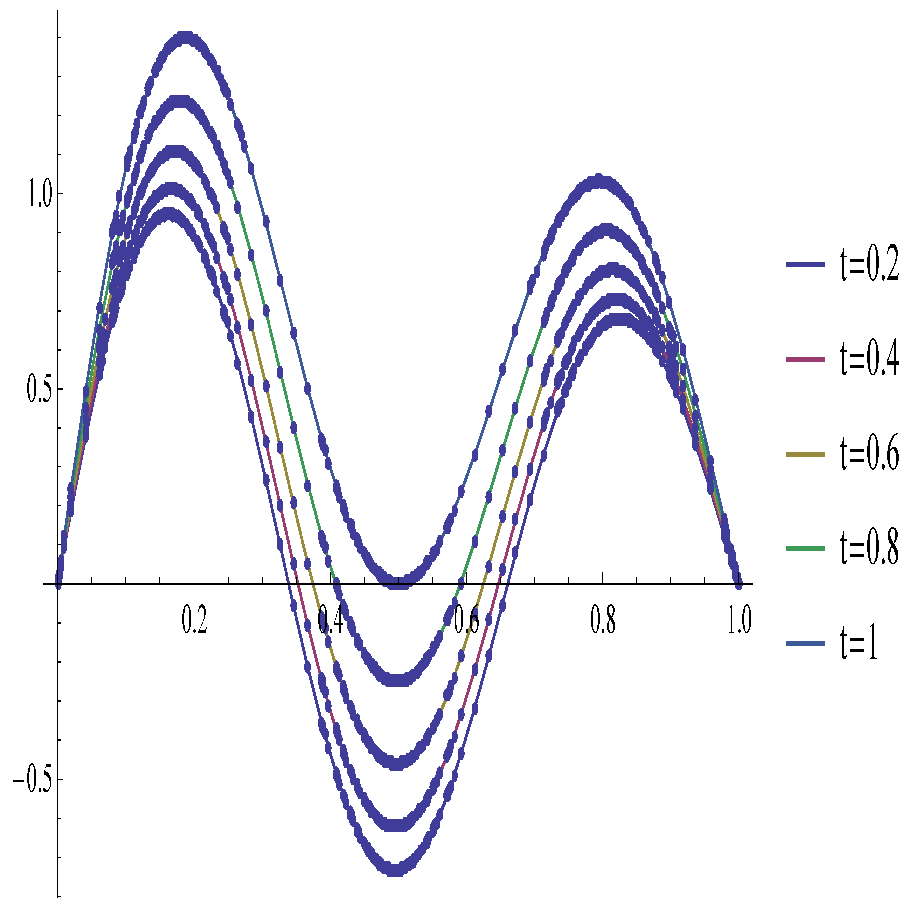
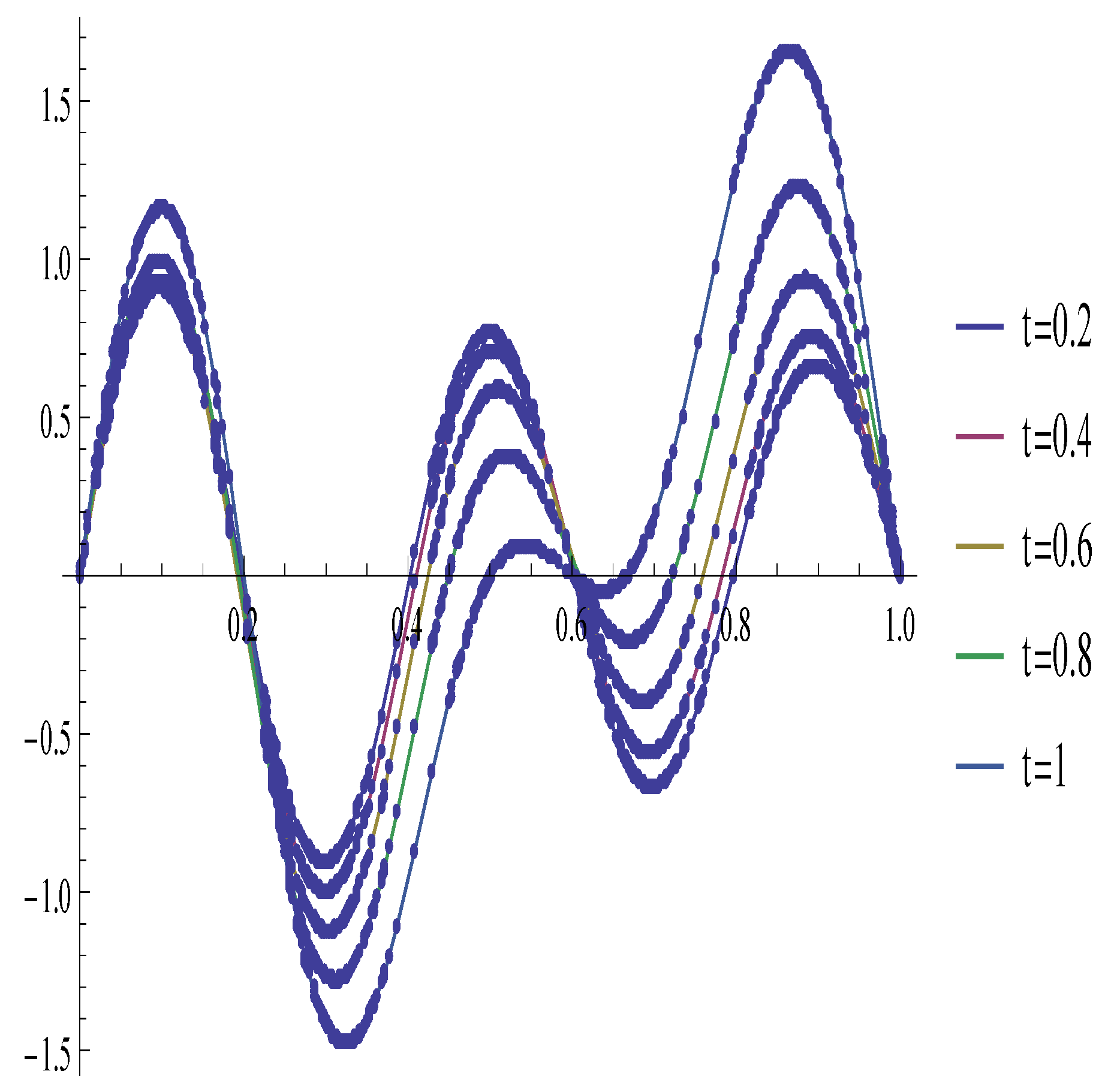
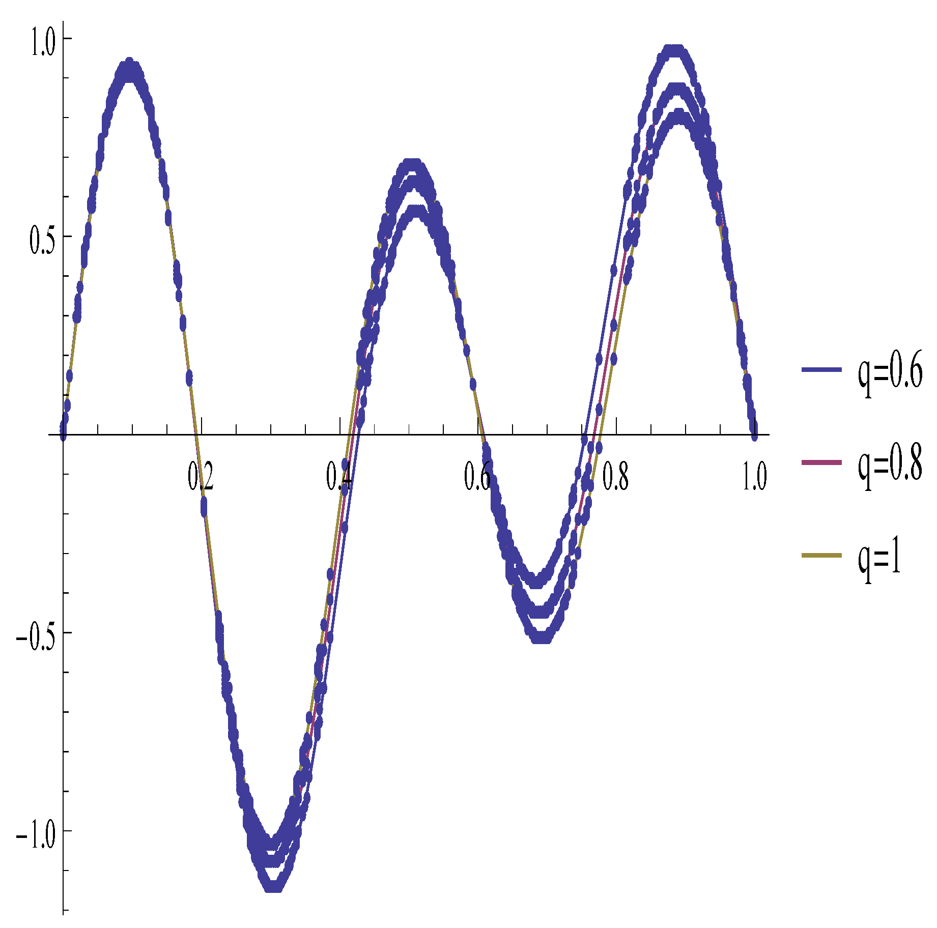
5. Illustrative Examples

In this section, we discuss several examples to explain the previous discussion. The first example will be about Theorem 7. We find the exact solution to the one-dimensional fractional IDEs with constant coefficients. Then, we will discuss the behavior of the solution when q approaches one.

Example 1.

Consider the following one-dimensional fractional IDE of the form

$$D^{2q}r\left(t\right)+{\alpha }_1{D}^{q}r\left(t\right)+{\alpha }_{2}r\left(t\right)+{\alpha }_3{I}^{q}r\left(t\right)=0$$

(123)

with

$$r\left(0\right)=1,D^{q}r\left(0\right)=1.$$

(124)

We will consider four cases:

1. 

If ${\alpha }_1=-3,{\alpha }_2=4$, and ${\alpha }_3=-2$, then the roots of $z^3+{\alpha }_1{z}^2+{\alpha }_{2}z+{\alpha }_3=0$ are $1,1\pm i$. Using the first part of Theorem 7, $c_1=-1,c_2=-2$ and $c_3=2$. Then, the solution of Equations (123) and (124) will be

$$r_q\left(t\right)=-E_q\left(t^q\right)+2{\cos }_q\left((1+i)t^q\right).$$

(125)

Then,

$$\begin{array}{ccc}\hfill \underset{q\to 1}{\lim }{r}_q\left(t\right)& =& \underset{q\to 1}{\lim }(-E_q\left(t^q\right)+2{\cos }_q\left((1+i)t^q\right))\hfill \end{array}$$

(126)

$$\begin{array}{ccc}& =& -e^t+2e^{t}cost,\hfill \end{array}$$

(127)

which is the solution of

$$r^{″}\left(t\right)-3r^{\prime }\left(t\right)+4r\left(t\right)-2{\int }_0^{t}r\left(s\right)ds=0,r\left(0\right)=r^{\prime }\left(0\right)=1.$$

(128)

Note that

$$\begin{array}{ccc}& & \underset{q\to 1}{\lim }{E}_q\left(\lambda t^q\right)=e^{\lambda t},\underset{q\to 1}{\lim }{\cos }_q\left((\mu +i\nu )t^q\right))=e^{\mu t}\cos \left(\nu t\right),\hfill \end{array}$$

(129)

$$\begin{array}{ccc}& & \underset{q\to 1}{\lim }{\sin }_q\left((\mu +i\nu )t^q\right))=e^{\mu t}\sin \left(\nu t\right).\hfill \end{array}$$

(130)

2. 

If ${\alpha }_1=-6,{\alpha }_2=11$, and ${\alpha }_3=-6$, then the roots of $z^3+{\alpha }_1{z}^2+{\alpha }_{2}z+{\alpha }_3=0$ are $1,2,3$. Using the second part of Theorem 7, we obtain the result that $c_1=-2,c_2=6$, and $c_3=-3$. Then, the solution of Equations (123) and (124) will be

$$r_q\left(t\right)=-2E_q\left(t^q\right)+6E_q\left(2t^q\right)-3E_q\left(3t^q\right).$$

(131)

Then,

$$\begin{array}{ccc}\hfill \underset{q\to 1}{\lim }{r}_q\left(t\right)& =& \underset{q\to 1}{\lim }(-2E_q\left(t^q\right)+6E_q\left(2t^q\right)-3E_q\left(3t^q\right))\hfill \end{array}$$

(132)

$$\begin{array}{ccc}& =& -2e^t+6e^{2t}-3e^{3t},\hfill \end{array}$$

(133)

which is the solution of

$$r^{″}\left(t\right)-6r^{\prime }\left(t\right)+11r\left(t\right)-6{\int }_0^{t}r\left(s\right)ds=0,r\left(0\right)=r^{\prime }\left(0\right)=1.$$

(134)

3. 

If ${\alpha }_1=-4,{\alpha }_2=5$, and ${\alpha }_3=-2$, then the roots of $z^3+{\alpha }_1{z}^2+{\alpha }_{2}z+{\alpha }_3=0$ are $1,1,2$. Using the third part of Theorem 7, $c_1=3,c_2=2$ and $c_3=-2$. Then, the solution of Equations (123) and (124) will be

$$r_q\left(t\right)=3E_q\left(t^q\right)+\frac{2t^q}{q}{E}_{q,q}\left(t^q\right)-2E_q\left(2t^q\right).$$

(135)

Then,

$$\begin{array}{ccc}\hfill \underset{q\to 1}{\lim }{r}_q\left(t\right)& =& \underset{q\to 1}{\lim }(3E_q\left(t^q\right)+\frac{2t^q}{q}{E}_{q,q}\left(t^q\right)-2E_q\left(2t^q\right))\hfill \end{array}$$

(136)

$$\begin{array}{ccc}& =& 3e^t+2t{e}^t-2e^{2t},\hfill \end{array}$$

(137)

which is the solution of

$$r^{″}\left(t\right)-4r^{\prime }\left(t\right)+5r\left(t\right)-2{\int }_0^{t}r\left(s\right)ds=0,r\left(0\right)=r^{\prime }\left(0\right)=1.$$

(138)

4. 

If ${\alpha }_1=-3,{\alpha }_2=3$, and ${\alpha }_3=-1$, then the roots of $z^3+{\alpha }_1{z}^2+{\alpha }_{2}z+{\alpha }_3=0$ are $1,1,1$. Using the fourth part of Theorem 7, we find that $c_1=1,c_2=0$, and $c_3=-1$. Then, the solution of Equations (123) and (124) will be

$$r_q\left(t\right)=E_q\left(t^q\right)-E_q\left(t^q\right)\ast \left(t^{2q-1}G{E}_q\left(t^q\right)\right).$$

(139)

Then,

$$\begin{array}{ccc}\hfill \underset{q\to 1}{\lim }{r}_q\left(t\right)& =& \underset{q\to 1}{\lim }(E_q\left(t^q\right)-E_q\left(t^q\right)\ast \left(t^{2q-1}G{E}_q\left(t^q\right)\right)\hfill \end{array}$$

(140)

$$\begin{array}{ccc}& =& e^t-e^t\ast t{e}^t=e^t-\frac{1}{2}{t}^2{e}^t\hfill \end{array}$$

(141)

which is the solution of

$$r^{″}\left(t\right)-3r^{\prime }\left(t\right)+3r\left(t\right)-{\int }_0^{t}r\left(s\right)ds=0,r\left(0\right)=r^{\prime }\left(0\right)=1.$$

(142)

Note that

$$\begin{array}{c}\hfill \underset{q\to 1}{\lim }G{E}_q\left(t^q\right))=\sum _{j=0}^{\infty }\frac{(j+1)t^j}{\mathsf{\Gamma }(j+2)}=\sum _{j=0}^{\infty }\frac{(j+1)t^j}{(j+1)!}=e^t.\end{array}$$

(143)

Now, we will show how we can implement Theorem 8.

Example 2.

Consider the following two-dimensional fractional IDE of the form

$$w_{xx}(x,t)+D_t^{2q}w(x,t)-3D_t^{q}w(x,t)+w_x(x,t)+3w(x,t)-I_t^{q}w(x,t)=0$$

(144)

with

$$w(0,t)=w(1,t)=0,t\ge 0$$

(145)

and

$$w(x,0)=e^{\frac{-1}{2}x}\sin \left(\pi x\right),D^{q}w(x,0)=e^{\frac{-1}{2}x}\sin \left(2\pi x\right),0\le x\le 1.$$

(146)

Theorem 8 gives the result that the solution of Equations (144)–(146) has the following form

$$w(x,t)=\sum _{n=1}^{\infty }{e}^{\frac{-1}{2}x}{r}_n\left(t\right)sin\left(n\pi x\right)$$

(147)

where $r_n\left(t\right)$ satisfies the equation

$$D_t^{2q}{r}_n\left(t\right)-3D_t^q{r}_n\left(t\right)+\left(3-\frac{4n^2{\pi }^2+1}{4}\right)r_n\left(t\right)-I_t^q{r}_n\left(t\right)=0.$$

(148)

The initial conditions in Equation (146) give

$$r_n\left(0\right)=\left\{\begin{array}{cc}1,\hfill & n=1\hfill \\ 0,\hfill & n>1\hfill \end{array}\right.,D^q{r}_n\left(0\right)=\left\{\begin{array}{cc}1,\hfill & n=2\hfill \\ 0,\hfill & n=1orn>2\hfill \end{array}\right..$$

(149)

Simple calculations imply that the equation $z^3-3z^2+\left(3-\frac{4n^2{\pi }^2+1}{4}\right)z-1=0$ has one real root

$$\begin{array}{ccc}& & {\lambda }_n=-\frac{{\gamma }_n}{12\sqrt[3]{2}}-\frac{12\sqrt[3]{2}}{{\gamma }_n}+1,\hfill \end{array}$$

(150)

and two complex roots

$$\begin{array}{c}\hfill {\mu }_n\pm i{\nu }_n=1+\frac{6\sqrt[3]{2}}{{\gamma }_n}+\frac{{\gamma }_n}{24\sqrt[3]{2}}\pm i\left(\frac{6\sqrt[3]{2}\sqrt{3}}{{\gamma }_n}-\frac{a}{8\sqrt[3]{2}\sqrt{3}}\right)\end{array}$$

(151)

where

$${\gamma }_n=\sqrt[3]{-1728{\pi }^2{n}^2+\sqrt{{\left(-1728{\pi }^2{n}^2-432\right)}^2-11943936}-432}.$$

(152)

for $n>2$, ${\beta }_{1,n}=r_n\left(0\right)=0$, and ${\beta }_{2,n}=D^q{r}_n\left(0\right)=0$. Using the first part of Theorem 8, we have

$$r_n\left(t\right)=0,n>2.$$

(153)

for $n=1$, ${\beta }_{1,1}=r_1\left(0\right)=1$, and ${\beta }_{2,1}=D^q{r}_n\left(0\right)=0$. Using the first part of Theorem 8, we have

$$\begin{array}{c}\hfill c_1=0.127535,c_2=0.0790346,c_3=0.872465.\end{array}$$

(154)

Thus,

$$\begin{array}{ccc}& & r_1\left(t\right)=0.127535E_q\left(3.61971t^q\right)-0.191303{\sin }_q\left((-0.309854+1.46532i)t^q\right)\hfill \end{array}$$

(155)

$$\begin{array}{ccc}& & +0.872465{\cos }_q\left((-0.309854+1.46532i)t^q\right).\hfill \end{array}$$

(156)

For $n=2$, ${\beta }_{1,1}=r_1\left(0\right)=0$ and ${\beta }_{2,1}=D^q{r}_n\left(0\right)=1$. Using the first part of Theorem 8, we have

$$\begin{array}{c}\hfill c_1=0.123247,c_2=0.210087,c_3=-0.123247.\end{array}$$

(157)

Thus,

$$\begin{array}{ccc}& & r_2\left(t\right)=0.123247E_q\left(4.7046t^q\right)+0.31513{\sin }_q\left((-0.852301-2.70057i)t^q\right)\hfill \end{array}$$

(158)

$$\begin{array}{ccc}& & -0.123247{\cos }_q\left((-0.852301-2.70057i)t^q\right).\hfill \end{array}$$

(159)

Therefore, the solution of the Problem (144)–(146) is given by

$$\begin{array}{c}\hfill w_q(x,t)=e^{\frac{-1}{2}x}\sin \left(\pi x\right)r_1\left(t\right)+e^{\frac{-1}{2}x}\sin \left(2\pi x\right)r_2\left(t\right).\end{array}$$

(160)

In the next two examples, we will test our numerical approach described in Section 3.

Example 3.

Consider the following two-dimensional fractional IDE of the form

$$w_{xx}(x,t)+D_t^{7/4}w(x,t)-2D_t^{7/8}w(x,t)+w_x(x,t)+3w(x,t)-4I_t^{7/8}w(x,t)=g(x,t)$$

(161)

with

$$w(0,t)=w(1,t)=0,t\ge 0$$

(162)

and

$$w(x,0)=e^{\frac{-1}{2}x}\sin \left(3\pi x\right),D^{q}w(x,0)=0,0\le x\le 1$$

(163)

where

$$\begin{array}{ccc}\hfill g(x,t)& =& \left(\left(11-4{\pi }^2\right)t^{7/4}-\frac{8t^{7/8}\mathsf{\Gamma }\left(\frac{11}{4}\right)}{\mathsf{\Gamma }\left(\frac{15}{8}\right)}-\frac{16t^{21/8}\mathsf{\Gamma }\left(\frac{11}{4}\right)}{\mathsf{\Gamma }\left(\frac{29}{8}\right)}+4\mathsf{\Gamma }\left(\frac{11}{4}\right)\right)\sin \left(\pi x\right)\hfill \end{array}$$

(164)

$$\begin{array}{ccc}& +& \frac{1}{4}{e}^{-\frac{x}{2}}\left(-\frac{16t^{7/8}}{\mathsf{\Gamma }\left(\frac{15}{8}\right)}-36{\pi }^2+11\right)\sin \left(3\pi x\right).\hfill \end{array}$$

(165)

Then, the exact solution is

$$w(x,t)=t^{7/4}{e}^{-\frac{x}{2}}\sin \left(\pi x\right)+e^{-\frac{x}{2}}\sin \left(3\pi x\right).$$

(166)

Here, we use $M_1=M_2=40.$ Then, the absolute error is defined by

$$ϵ(x,t)=\mid w(x,t)-w_{40,40}(x,t)\mid .$$

(167)

The absolute errors for different values of x and t are reported in

Table 1. The absolute errors for different values of x and t for Example 3.

x	$\mathit{ϵ}(\mathit{x},0.25)$	$\mathit{ϵ}(\mathit{x},0.5)$	$\mathit{ϵ}(\mathit{x},0.75)$
0	0	0	0
0.2	$3.12\ast {10}^{-14}$	$3.00\ast {10}^{-14}$	$3.74\ast {10}^{-14}$
0.4	$3.94\ast {10}^{-14}$	$3.28\ast {10}^{-14}$	$3.81\ast {10}^{-14}$
0.6	$4.11\ast {10}^{-14}$	$3.50\ast {10}^{-14}$	$3.99\ast {10}^{-14}$
0.8	$4.38\ast {10}^{-14}$	$3.85\ast {10}^{-14}$	$4.17\ast {10}^{-14}$
1	$4.97\ast {10}^{-14}$	$3.22\ast {10}^{-14}$	$4.31\ast {10}^{-14}$

.

We also compute the $L_2$-error, which is given by

$${ϵ}_{L_2}=\sqrt{{\int }_0^1{\int }_0^1\mid w(x,t)-w_{40,40}(x,t){\mid }^{2}dxdt}=2.84\ast {10}^{-13}.$$

(168)

In addition, the graphs of the exact and approximate solutions for t = 0.2, 0.4, 0.6, 0.8, 1 are given in Figure 1. The dot points are the approximate solutions, and the solid lines are the exact solutions.

We discuss another example with ${\nu }_2\left(t\right)$ is a non-constant function.

Example 4.

Consider the following two-dimensional fractional IDE of the form

$$w_{xx}(x,t)+D_t^{2q}w(x,t)-D_t^{q}w(x,t)+w_x(x,t)+(t^q+1)w(x,t)-I_t^{q}w(x,t)=g(x,t)$$

(169)

with

$$w(0,t)=w(1,t)=0,t\ge 0$$

(170)

and

$$w(x,0)=e^{\frac{-1}{2}x}\sin \left(5\pi x\right),D^{q}w(x,0)=0,0\le x\le 1$$

(171)

where

$$\begin{array}{ccc}\hfill g(x,t)& =& \frac{4e^{-\frac{x}{2}}{t}^q(\mathsf{\Gamma }(2q+1)\sin \left(2\pi x\right)+\mathsf{\Gamma }(3q+1)\sin \left(3\pi x\right)-\sin \left(5\pi x\right))}{4\mathsf{\Gamma }(q+1)}\hfill \end{array}$$

(172)

$$\begin{array}{ccc}& +& \frac{e^{-\frac{x}{2}}\left(4\mathsf{\Gamma }{(2q+1)}^2\sin \left(2\pi x\right)\left(t^{3q}-\mathsf{\Gamma }(3q+1)\right)-4t^{2q}\mathsf{\Gamma }{(3q+1)}^2\sin \left(3\pi x\right)\right)}{4\mathsf{\Gamma }(2q+1)\mathsf{\Gamma }(3q+1)}\hfill \end{array}$$

(173)

$$\begin{array}{ccc}& +& \frac{e^{-\frac{x}{2}}\left(\mathsf{\Gamma }(4q+1)\left(-t^{2q}\left(4t^q-16{\pi }^2+3\right)\sin \left(2\pi x\right)\right)-4t^{4q}\mathsf{\Gamma }(3q+1)\sin \left(3\pi x\right)\right)}{4\mathsf{\Gamma }(4q+1)}\hfill \end{array}$$

(174)

$$\begin{array}{ccc}& +& \frac{e^{-\frac{x}{2}}{t}^{3q}\left(\left(4t^q-36{\pi }^2+3\right)\sin \left(3\pi x\right)+\left(4t^q-100{\pi }^2+3\right)\sin \left(5\pi x\right)\right)}{4\mathsf{\Gamma }(4q+1)}.\hfill \end{array}$$

(175)

Then, the exact solution is

$$w(x,t)=-e^{-\frac{x}{2}}{t}^{2q}\sin \left(2\pi x\right)+e^{-\frac{x}{2}}{t}^{3q}\sin \left(3\pi x\right)+e^{-\frac{x}{2}}\sin \left(5\pi x\right).$$

(176)

Here, we use $M_1=M_2=40.$ Then, the absolute error for the fractional derivative of order q is defined by

$${ϵ}_q(x,t)=\mid w(x,t)-w_{40,40}(x,t)\mid .$$

(177)

The absolute errors for different values of x and t are reported in

Table 2. The absolute errors for different values of x and t for Example 4.

x	${\mathit{ϵ}}_{\frac{3}{4}}(\mathit{x},0.25)$	${\mathit{ϵ}}_{\frac{3}{4}}(\mathit{x},0.5)$	${\mathit{ϵ}}_{\frac{3}{4}}(\mathit{x},0.75)$
0	0	0	0
0.2	$4.23\ast {10}^{-14}$	$4.51\ast {10}^{-14}$	$4.11\ast {10}^{-14}$
0.4	$4.79\ast {10}^{-14}$	$4.72\ast {10}^{-14}$	$4.38\ast {10}^{-14}$
0.6	$4.91\ast {10}^{-14}$	$4.89\ast {10}^{-14}$	$4.83\ast {10}^{-14}$
0.8	$5.34\ast {10}^{-14}$	$5.21\ast {10}^{-14}$	$5.32\ast {10}^{-14}$
1	$5.80\ast {10}^{-14}$	$5.42\ast {10}^{-14}$	$5.55\ast {10}^{-14}$

.

We also compute the $L_2$-error, which is given by

$${ϵ}_{L_2}\left(q\right)=\sqrt{{\int }_0^1{\int }_0^1\mid w(x,t)-w_{40,40}(x,t){\mid }^{2}dxdt}.$$

(178)

The $L_2$- errors for different values of q are reported in

Table 3. The $L_2$- errors for different values of q for Example 4.

q	${\mathit{ϵ}}_{{\mathit{L}}_2}\left(\mathit{q}\right)$
$\frac{3}{4}$	$4.23\ast {10}^{-13}$
$\frac{7}{8}$	$4.48\ast {10}^{-13}$
$\frac{8}{9}$	$4.51\ast {10}^{-13}$
$\frac{10}{11}$	$4.42\ast {10}^{-13}$

.

Additionally, the graphs of the exact and approximate solutions for $t=0.2,0.4,0.6,0.8,1$ for $q=\frac{9}{10}$ are given in Figure 2. The dot points are the approximate solutions, and the solid lines are the exact solutions.

We also show the graph of exact and approximate solutions at $t=0.5$ for different values of q in Figure 3.

6. Conclusions

This article is divided into two main parts. In the first part, we use OMM to numerically explore the 2D fractional IDE. We derive a numerical approach and present a proof of these operational matrices. We test the numerical method on some examples to show its efficiency. Results are shown in Examples 1 and 2. We use various methods to measure the errors of the approximation, such as absolute and $L_2$ errors. In addition, we explore the effect of derivative order. Note the following when using these two examples:

1.

The absolute error for different values of x and t is on the order of ${10}^{-14}$, which is very small, as seen in Table 1 and Table 2.

2.

The $L_2$ error is also on the order of ${10}^{-13}$ and is very small, as shown in Table 3.

3.

Approximate and exact solutions for various values of t agree, as shown in Figure 1 and Figure 2.

4.

As shown in Figure 3, the approximate solution for the derivative order q converges to the solution for $q=1$.

Part 2 examines the exact solutions for 1D and 2D fractional IDEs. We use the fractional Laplace transform to generate these exact solutions. All homogeneous cases are considered. We provide two examples for two purposes. First, we show how the results obtained are implemented, especially the exact solution for some 1D and 2D IDE classes. We then show that the exact fractional solution converges to the exact solution of the ordinary derivative as the order of the fractional derivative approaches one. These results are reported in Examples 3 and 4. Note that this work uses sequential Caputo derivative. It helps us fluently implement numerical and analytical approaches. In this paper, we show that our approach works efficiently for these types of problems. This can be generalized to other types of fractional IDEs and other scientific and engineering applications.

References

1. Miller, K.S.; Ross, B. An Introduction to the Fractional Calculus and Fractional Differential Equations; John Wiley & Sons: Hoboken, NJ, USA, 1993; Volume 6. [Google Scholar]
2. Podlubny, I. Fractional Differential Equations: An Introduction to Fractional Derivatives, Fractional Differential Equations, to Methods of Their Solution and Some of Their Applications; Elsevier: Amsterdam, The Netherlands, 1999; Volume 198. [Google Scholar]
3. Kilbas, A.A.; Srivastava, H.M.; Trujillo, J.J. Theory and Applications of Fractional Differential Equations; Elsevier: Amsterdam, The Netherlands, 2006; Volume 204. [Google Scholar]
4. Zhang, S.; Wei, T. Sequential fractional derivative: Definition and its properties. J. Math. Anal. Appl. 2009, 353, 441–446. [Google Scholar]
5. Atanackovic, T.M.; Pilipovic, S. On sequential fractional derivatives in the Caputo sense. Appl. Math. Comput. 2010, 216, 3452–3460. [Google Scholar]
6. Li, X.; Liu, F.; Yang, X.J.; Baleanu, D. Sequential fractional derivative models and applications. Chaos Solitons Fractals 2021, 143, 110739. [Google Scholar]
7. Zhong, W.P.; Chen, Y.Q.; Sun, X.J.; Wei, X.J. On the sequential fractional derivative and its application to fractional partial differential equations. Commun. Nonlinear Sci. Numer. Simul. 2019, 74, 257–268. [Google Scholar]
8. Baleanu, D.; Gülsu, M.; Mohammadi, H. On the non-commutativity of sequential fractional derivatives. Appl. Math. Lett. 2013, 26, 393–397. [Google Scholar]
9. Zhang, H.; Li, Y.; Shen, Y. An efficient and accurate numerical method for solving multi-term fractional differential equations based on sequential fractional derivatives. J. Comput. Phys. 2020, 409, 109346. [Google Scholar]
10. Columbu, A.; Frassu, S.; Viglialoro, G. Refined criteria toward boundedness in an attraction-repulsion chemotaxis system with nonlinear productions. Appl. Anal. 2023, 1–17. [Google Scholar] [CrossRef]
11. Li, T.; Frassu, S.; Viglialoro, G. Combining effects ensuring boundedness in an attraction–repulsion chemotaxis model with production and consumption. Z. Angew. Math. Phys. 2023, 74, 109. [Google Scholar] [CrossRef]
12. Volterra, V. Theory of Functionals and of Integral and Integro-Differential Equations; Dover Publications: Mineola, NY, USA, 1913. [Google Scholar]
13. Baleanu, D.; Diethelm, K.; Scalas, E.; Trujillo, J.J. (Eds.) Fractional Calculus Models and Numerical Methods; World Scientific: Singapore, 2012; Volume 3. [Google Scholar]
14. Wang, Y.; Sun, H.; Li, C. Stability analysis of fractional differential equations with Caputo derivative. Commun. Nonlinear Sci. Numer. Simul. 2012, 17, 1318–1326. [Google Scholar] [CrossRef]
15. Wu, G.C.; Liao, S.J. An efficient approach to obtain higher-order approximations of fractional derivatives by the generalized Taylor matrix method. J. Vib. Control 2012, 18, 1013–1023. [Google Scholar]
16. Canuto, C.; Hussaini, M.Y.; Quarteroni, A.; Zang, T.A. Spectral Methods: Fundamentals in Single Domains; Springer Science & Business Media: Berlin/Heidelberg, Germany, 2006. [Google Scholar]
17. Abuasbeh, K.; Kanwal, A.; Shafqat, R.; Taufeeq, B.; Almulla, M.A.; Awadalla, M. A Method for Solving Time-Fractional Initial Boundary Value Problems of Variable Order. Symmetry 2023, 15, 519. [Google Scholar] [CrossRef]
18. Abuasbeh, K.; Shafqat, R.; Alsinai, A.; Awadalla, M. Analysis of the Mathematical Modelling of COVID-19 by Using Mild Solution with Delay Caputo Operator. Symmetry 2023, 15, 286. [Google Scholar] [CrossRef]
19. Dallashi, Q.; Syam, M.I. An Efficient Method for Solving Second-Order Fuzzy Order Fuzzy Initial Value Problems. Symmetry 2022, 14, 1218. [Google Scholar] [CrossRef]
20. Tayeb, M.; Boulares, H.; Moumen, A.; Imsatfia, M. Processing Fractional Differential Equations Using ψ-Caputo Derivative. Symmetry 2023, 15, 955. [Google Scholar] [CrossRef]
21. Podlubny, I. Fractional Differential Equations; Academic Press: San Diego, CA, USA, 1999. [Google Scholar]
22. Baleanu, D.; Mustafa, O.G. On the solutions of sequential fractional differential equations. J. Comput. Nonlinear Dyn. 2013, 8, 031012. [Google Scholar]
23. Vatsala, A.S.; Pageni, G.; Vijesh, V.A. Analysis of Sequential Caputo Fractional Differential Equations versus Non-Sequential Caputo Fractional Differential Equations with Applications. Foundations 2022, 2, 1129–1142. [Google Scholar] [CrossRef]
24. Alomari, A.K.; Baleanu, D.; Al-Smadi, M.O. An efficient operational matrix method for solving multi-term time-fractional diffusion equations. Appl. Math. Comput. 2020, 367, 124820. [Google Scholar]
25. Syam, M.I.; Sharadga, M.; Hashum, I. A numerical method for solving fractional delay differential equations based on the operational matrix. Chaos Solitons Fractals 2021, 147, 110977. [Google Scholar] [CrossRef]
26. Kashkari, B.; Syam, M. Fractional-order Legendre operational matrix of fractional integration for solving the Riccati equation with fractional order. Appl. Math. Comput. 2016, 290, 281–291. [Google Scholar] [CrossRef]
Figure 1. The exact and approximate solutions for t = 0.2 , 0.4 , 0.6 , 8 , 1 .
Symmetry 15 01263 g001
Figure 2. The exact and approximate solutions for t = 0.2 , 0.4 , 0.6 , 8 , 1 .
Symmetry 15 01263 g002
Figure 3. The exact and approximate solutions at t = 0.5 for different values of q.
Symmetry 15 01263 g003