Article

Generalized Support Vector Regression and Symmetry Functional Regression Approaches to Model the High-Dimensional Data

1
Department of Statistics, Faculty of Mathematics, Statistics and Computer Sciences, Semnan University, P.O. Box 35195-363, Semnan 35131-19111, Iran
2
Institute of Mathematical Sciences, Faculty of Science, Universiti Malaya, Kuala Lumpur 50603, Malaysia
*
Authors to whom correspondence should be addressed.
Symmetry 2023, 15(6), 1262; https://doi.org/10.3390/sym15061262
Submission received: 15 March 2023 / Revised: 17 May 2023 / Accepted: 17 May 2023 / Published: 15 June 2023
(This article belongs to the Special Issue Symmetry in Multivariate Analysis)

Abstract

:
The analysis of the high-dimensional dataset when the number of explanatory variables is greater than the observations using classical regression approaches is not applicable and the results may be misleading. In this research, we proposed to analyze such data by introducing modern and up-to-date techniques such as support vector regression, symmetry functional regression, ridge, and lasso regression methods. In this study, we developed the support vector regression approach called generalized support vector regression to provide more efficient shrinkage estimation and variable selection in high-dimensional datasets. The generalized support vector regression can improve the performance of the support vector regression by employing an accurate algorithm for obtaining the optimum value of the penalty parameter using a cross-validation score, which is an asymptotically unbiased feasible estimator of the risk function. In this regard, using the proposed methods to analyze two real high-dimensional datasets (yeast gene data and riboflavin data) and a simulated dataset, the most efficient model is determined based on three criteria (correlation squared, mean squared error, and mean absolute error percentage deviation) according to the type of datasets. On the basis of the above criteria, the efficiency of the proposed estimators is evaluated.

1. Introduction

There are now a variety of methods for data collecting. High-dimensional datasets can be developed because of the nature of the data as well as the lower cost involved in data collection. This means that the number of explanatory variables (p) is greater than the number of observations (n) [1,2]. The multiple linear regression is a standard statistical technique in a researcher’s toolbox. The multiple linear regression model is given by Y = X β + ϵ where Y = ( y 1 , , y n ) is a response variable, X = ( x 1 , , x n ) is a design matrix that includes the predictor or explanatory variables, and ϵ = ( ϵ 1 , , ϵ n ) is a vector of error terms with E ( ϵ ) = 0 and Var ( ϵ ) = σ 2 I n . Furthermore, β = ( β 1 , , β p ) is an unknown p-dimensional vector of regression coefficients that describe the relationship between a predictor’s variable and the response. Implementing a linear regression is problematic in such data and the results are misleading. The estimation of coefficients using the least-squares method is in the following form:
β ^ = ( X X ) 1 X Y .
In high-dimensional cases, the inverse of X X does not exist, because the matrix is not the full rank. In this situation, different methods are proffered to analyze the data, and the best method is selected according to the time, accuracy, and cost (see [3,4,5]).
To analyze the high-dimensional data, due to the existence of many explanatory variables, it is possible that some of these variables are not related to the response variable. Hence, the principal component method is a common approach among the alternative methods to reduce the dimensions of explanatory variables.
In recent years, machine learning in data analysis has developed significantly, and many scientists resort to this method to solve high-dimensional problems in the datasets.
Among the various methods and algorithms that are available in the field of machine learning, support vector machines are one of the most important and widely used, and these are a powerful tool for data classification [6].
The support vector regression model has the advantage that it does not look for the minimum error, but seeks the optimal error. The optimal error is the error that makes the model more efficient and accurate. Aircraft control without a pilot, computer quality analysis, the design of artificial limbs, routing systems, etc., are some of the applications of this model. Therefore, in this method, there is a need for a system that can learn through training and pattern distinction in order to function properly in categorizing data. Some researchers have used machine learning algorithms to increase the predictive performance [7,8].
Functional data analysis is an important tool in statistical modeling, in which the behavior of the data is a function of another variable. The functional regression model is used in many fields such as meteorology, chemometrics, diffusion tensor imaging tractography, and other areas [9,10,11].
Based on [12,13,14,15], the criteria used to evaluate and compare the fitted models are the squared correlation between the estimated and real values of the response variable ( R 2 or R-squared), the root mean squared error (RMSE), and mean absolute percentage error (MAPE), which are defined as follows:
R 2 = C o v 2 ( Y i , Y ^ i ) V a r ( Y i ) V a r ( Y ^ i ) , RMSE = 1 T i = 1 T ( Y i Y ^ i ) 2 , MAPE = 1 T i = 1 T Y i Y ^ i Y i ,
where Y i is the real value of the response variable, Y ^ i is the predicted value of the response variable, and T is the total number of test samples. The models with higher values of R-squared and MAPE and the models with lower values of RMSE have a better fit to the data [16].

2. Materials and Methods

In this paper, a number of techniques for modeling high-dimensional data are introduced, and the best model is then chosen based on the estimation of the response variable and proposed criteria.

2.1. Principal Component Method

The principal component method is one of data reduction techniques that involves reducing the dimensions and conserving as much information as possible from the explanatory variables. The principal components have been organized in a non-correlational way so that a small number of components can demonstrate a significant percentage of the information in the primary explanatory variables. Selecting the adequate number of components is noteworthy and various methods have been proposed to select the appropriate number of these components. One of the methods of finding the best number of principal components is to retain enough components to reach a large percentage of the total variation of the original variables. Values between 70 % and 90 % are usually acceptable, although smaller values might be appropriate as the sample size increases. Another way is to exclude the principal components that have eigenvalues that are less than the mean value of eigenvalues. Plotting the scree diagram is an intuitive technique to find the best number of principal components. In this diagram, we plot the eigenvalue of each component ( λ i ) against i. The number of components selected is the value of i that corresponds to an “elbow” in the curve, i.e., a change in the slope from “steep” to “shallow”. It is important to notice that each of the proposed methods may provide different answers. The researcher can use the method according to the dataset substance.

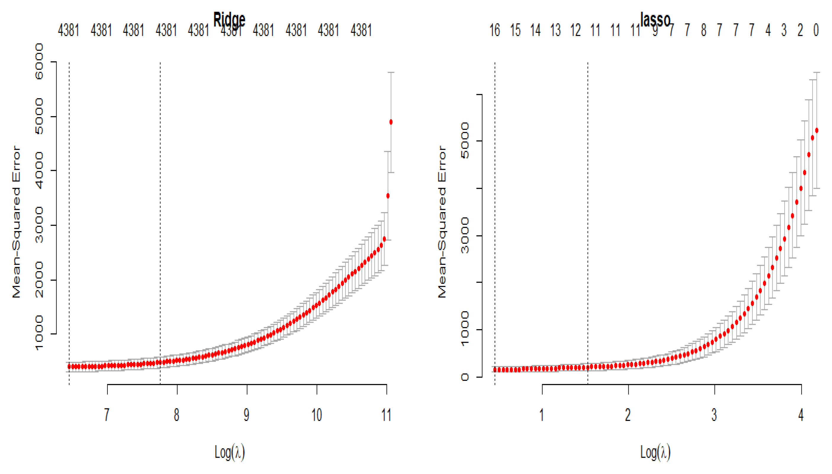
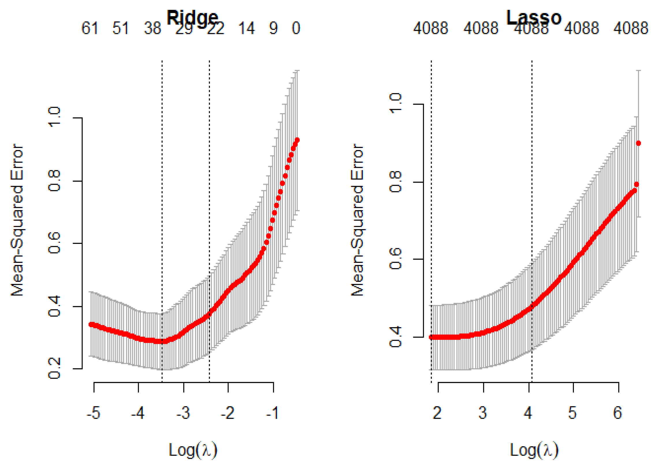
2.2. LASSO Regression

The basic motivation for the LASSO comes from an impressive method suggested by Breiman [4] that minimizes the non-negative garotte as follows:
i = 1 n Y i j = 1 p c j β ^ j X j i 2 c j 0 , j c j s
In this optimization problem, the estimators β ^ j are selected by the least square error. Parameter s is the penalty and when it is reduced, the garotte will tighten.
This method is renowned among researchers for the death penalty. In this method, some variables are deleted, and the rest are shrunk. In another form, the optimization problem of the LASSO regression can be presented as follows:
i = 1 n Y i j = 1 p X i j β j 2 + λ j = 1 p | β j | , i = 1 , , n , j = 1 , , p
One of the advantages of this method is the yielding to stable and continuous estimators [4]. One of the disadvantages of the LASSO method is that it has insufficient performance in correlated explanatory variables because it selects just one variable between correlated variables as a group and this is not the best reason. In a high-dimensional linear regression model, LASSO at most chooses n variables from p explanatory variables with n observations [17]. So, the effective explanatory variables may be removed.

2.3. Ridge Regression

Occasionally in regression models, the researchers encounter the collinearity between the explanatory variables, and this usually occurs in high-dimensional models. Andrei Nikolayevich Tikhonov, who is renowned for his important findings in topology, functional analysis, physics, and mathematics, presented the Tikhonov regularization as a solution to this ill-conditioned problem. Since X X is not invertible in high-dimensional cases, the least-squares regression method is not applicable. In this regard, the problem can be solved using the ridge method, in which positive value k is added to matrix X X . Although the ridge regression estimator of coefficients is biased, same as LASSO estimation, there are some values for k, in which the variance of the ridge estimation is less than the variance of the least-squares estimation, such that the mean-squared error of the ridge estimator is smaller than the variance of the least-squares estimator. The ridge estimator of β is calculated as follows:
β ^ = X X + k I 1 X Y , k 0 ,
where k is called the ridge parameter and its value is very important to find the appropriate model [18,19,20,21,22].

2.4. Functional Regression Model

Recently, due to the expansion of data types, modern technological innovations in data collection, data storage, and so on, the functional datasets are very observable and applicable [23]. This dataset uses many scientific fields. For example, neuroscientists look at patterns of functional connectivity between signals in different brain regions measured over time using magnetic resonance imaging in order to treat patients [24]. To analyze this type of dataset, firstly, it is necessary to convert the discrete dataset into the continuous dataset in order to apply one of the following methods.

Smoothing of Functional Data

At first, the discrete dataset must be converted into a continuous dataset, and this can be carried out by estimating a curve or a straight line using the smoothing method, such as the Fourier basis for periodical datasets and the spline approach for other datasets.
In general, under the assumption of the linear combination between the variables, the functional model can be considered as follows:
Y i = j = 1 k c j ϕ j ( t i ) + ϵ i = f ( t i ) + ϵ i ,
where f is a linear combination of the coefficients, ϕ j ’s are the basic functions and c j ’s are the coefficients. Overall, any vector in a vector space can be represented as a linear combination of the base vectors and any continuous function in a functional space can be written as a linear combination of the basic functions. The basic functions can be represented by one of the following cases:
  • Fourier basis:
    The majority of the Fourier basis functions are used for a dataset that is periodical, such as weather datasets that denote that it is usually cold in winter and warm in summer. The Fourier bases are represented as follows:
    1 , sin ( ω t ) , cos ( ω t ) , sin ( 2 ω t ) , cos ( 2 ω t ) , , sin ( m ω t ) , cos ( m ω t ) ,
    where ω is called the frequency period and is equal to 2 π p , and p is the recurrence period. For instance, the recurring period for the weather dataset is 365 days;
  • Spline basis:
    The spline functions are polynomial functions that first divide a discrete dataset into equal parts and then fit the best curve to each part. If its degree is zero, it estimates using the vertical and horizontal lines, and if its degree is one, it computes linearly and the higher degrees are computed as a curve. In addition, the area of the curve that is at the junction can be smoothed, and the points that are located at the junction are called knots. If there are numerous knots, they cause a low bias, and a high variance will lead to a rough fitting of the graph. It is important to note that there must be at least one observation in each knot.
    Some other basis functions include the constant, power, exponential, etc. The non-parametric regression function can be demonstrated as follows:
    Y i = f ( t i ) + ϵ i , i = 1 , , n ,
    where the errors are independent and have an identical distribution with the zero mean and variance σ 2 . To estimate f ( t i ) , according to the basis functions, we have
    f ^ ( t i ) = j = 1 p c j ϕ j ( t i ) ,
    where ϕ j ( t ) is the basis function that depends on the type of data and c j are the coefficients. For estimating the functional coefficients, the sum of squares error is minimized as follows:
    H ( c ) = i = 1 n ( Y i f ( t i ) ) 2 = i = 1 n ( Y i j = 1 p c j ϕ j ( t i ) ) 2 .
    The above equation can be rewritten in matrix form
    H ( c ) = ( Y Φ c ) ( Y Φ c ) .
    According to the least squares problem, the solution of the above minimization problem is c ^ = ( Φ Φ ) 1 Φ Y . So, we have:
    Y ^ = c ^ Φ = Φ ( Φ Φ ) 1 Φ S Y = SY
    where S is called a smoothing matrix.
    Selecting the number of basis functions is very important because the small number of basis functions leads to a large bias value and small variance value that yield to the under-fitting of the fitted model, and a large number of basis functions leads to a small bias value and a large variance value that yield to the over fitting of the fitted model.

2.5. Support Vector Regression Approach

Although support vector machines (SVMs) are powerful tools in classification, they are not well known in regression. A support vector regression (SVR) is a model of support vector machines, that takes continuous values instead of discrete values in the response variables. In support vector machines, we know that when there is a small amount of data in the margin, the dividing line is appropriate, despite the fact that in the SVR, when there is more data in the margin, the model is outperformed. The purpose of this section is to fit a model on the data { x k , y k } k = 1 N using a support vector regression, in which the response variable is continuous. The support vector regression model is defined as:
y = f ( x , W ) = W x + b ,
where W is the coefficient of the support vector regression and b is the intercept.

2.5.1. The Kernel Tricks in the Support Vector Machine

If there is no linear boundary between the datasets, the data will be moved to a new space, a new linear boundary must be found for the data in that new space, and x must be changed to Φ ( x ) in the whole issue discussed above. Thus, all of the data enter a new space, so computing the inner product Φ ( x ) Φ ( x ) is very difficult, and it therefore introduces a new way to calculate the inner product without changing it to a new space.
One of these ways is to use the kernel trick. The four most popular kernels for SVMs are as follows:
  • Linear kernel: The simplest kernel function is the product of the inner product of < x , y > plus an optional constant value of c as the intercept:
    k ( x , y ) = x y + c ;
  • Polynomial kernel: When all training data are normalized, the polynomial kernel is appropriate. Its kernel form is as follows:
    k ( x , y ) = ( α x y + c ) d ,
    where the parameters intercept (c), slope ( α ), and the degree of polynomials (d) can be adjusted according to the data;
  • Gaussian kernel: A sample of a radial function and its kernel are as follows:
    k ( x , y ) = e x p x y 2 2 σ 2 ,
    where parameter σ is adjustable and significantly determines the smoothness of the Gaussian kernel;
  • Sigmoid kernel: It is known as a multilayer perceptron (MLP) kernel. The sigmoid kernel originates from the neural network technique, where the bipolar sigmoid function is often utilized as an activation function for artificial neurons. This kernel function is defined as follows:
    k ( x , y ) = tanh ( α x y + c ) ,
    in which there are two adjustable parameters, the slope ( α ) and the intercept (c).
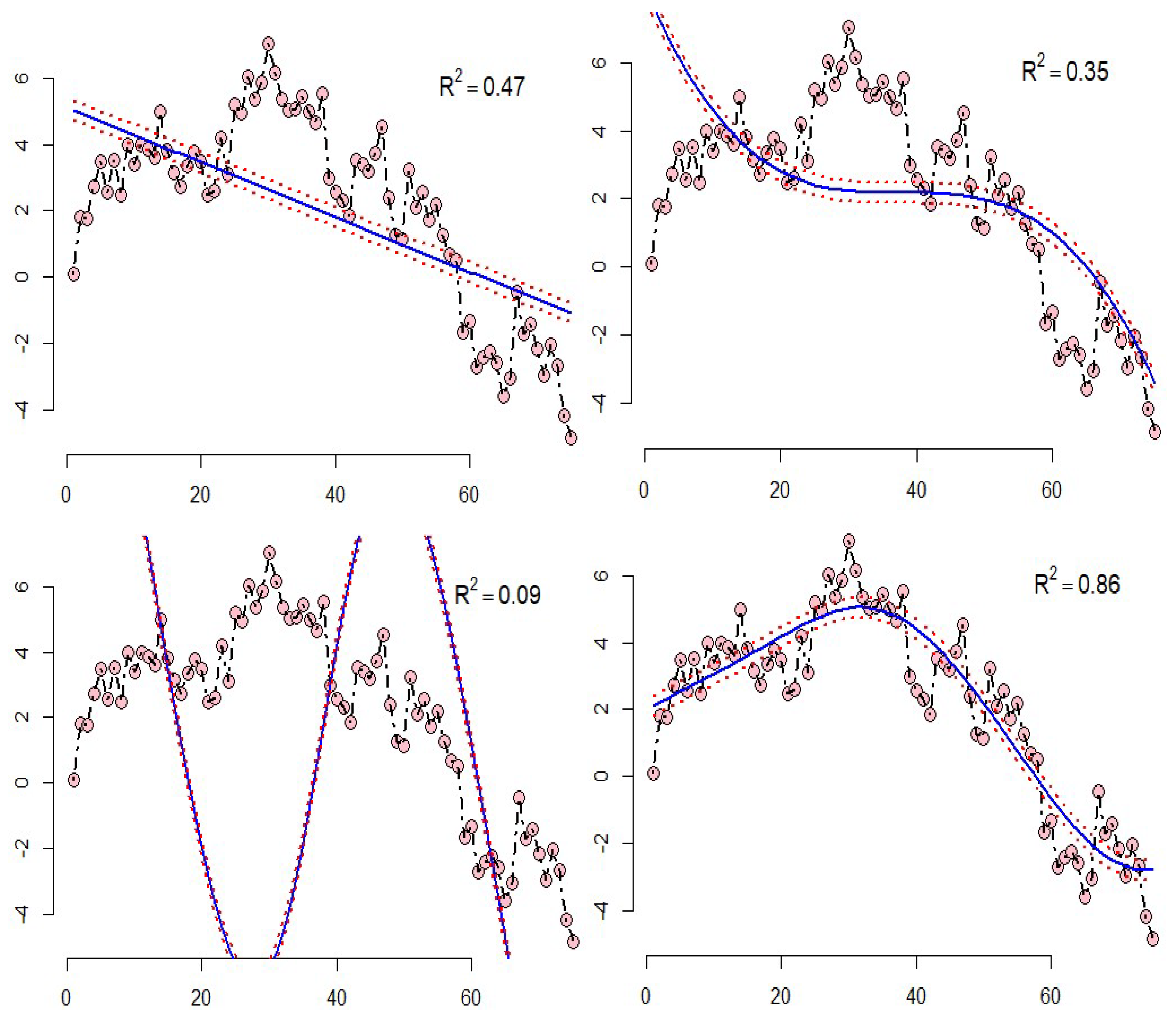
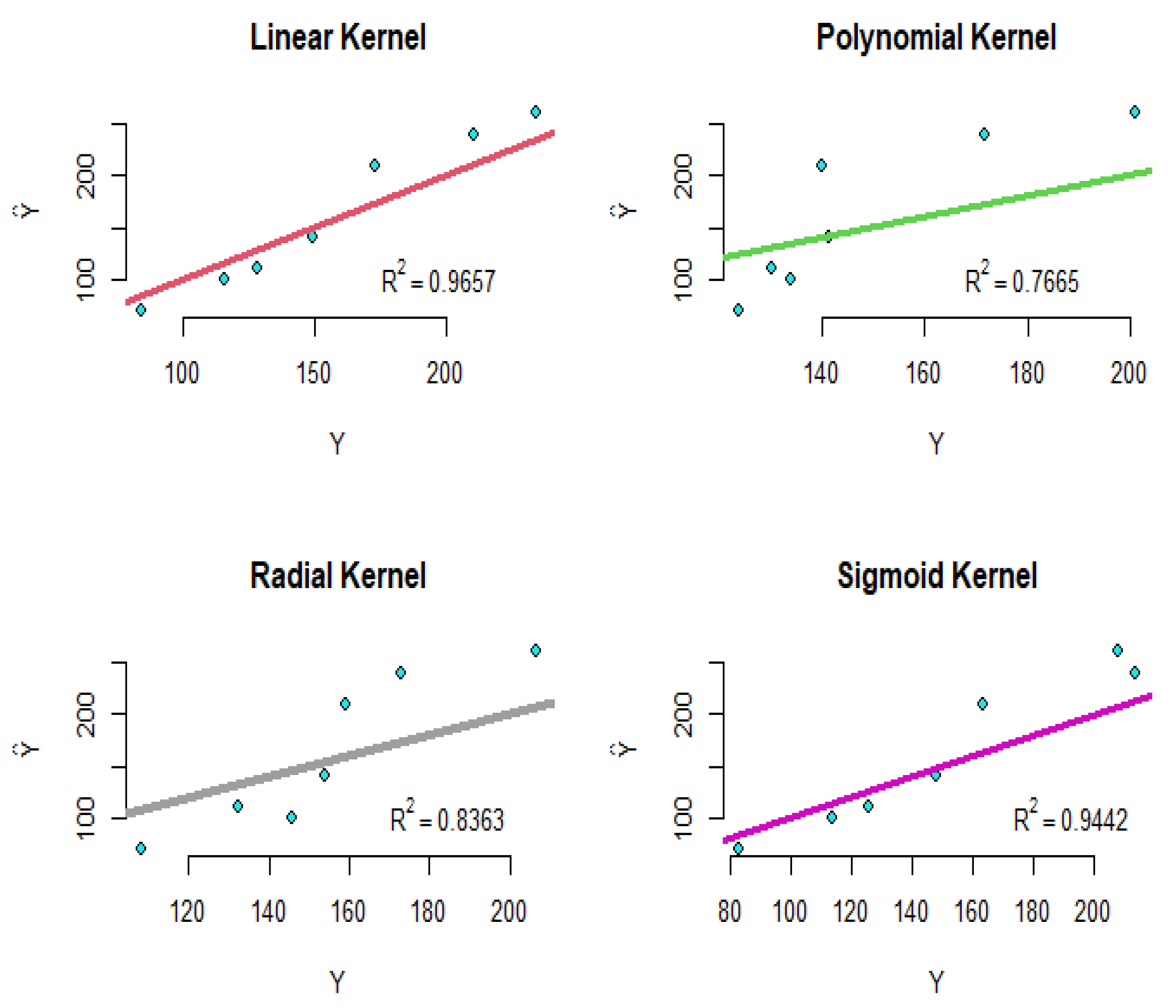
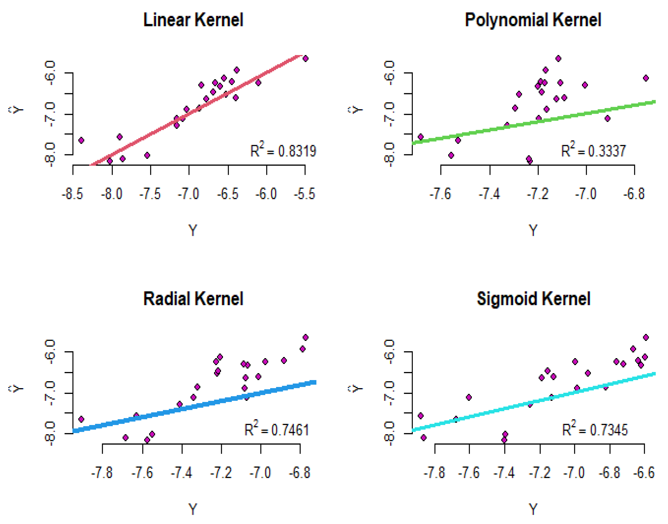
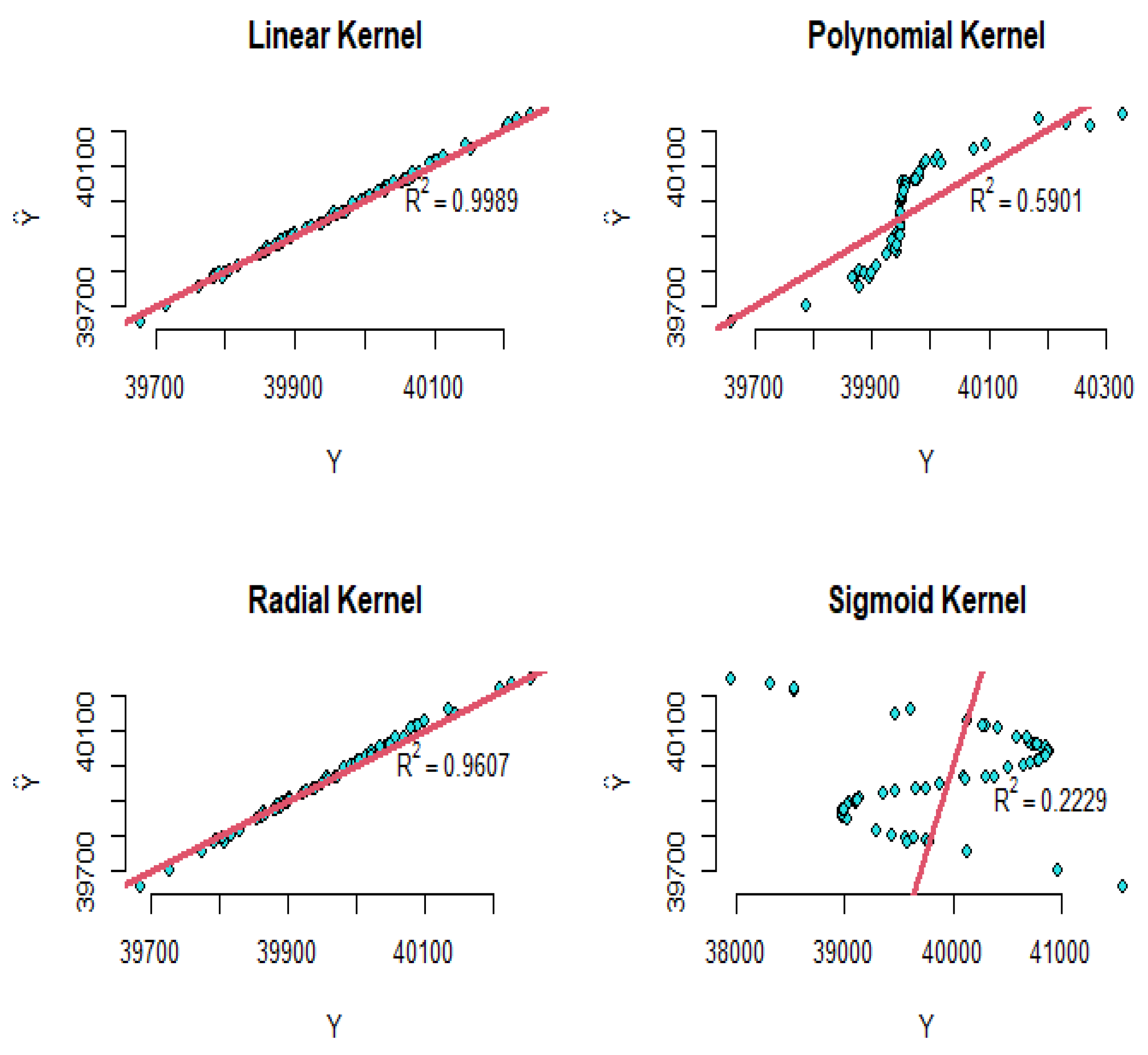
  • Example 1: The results of the SVR for the two-dimensional data, which is simulated with the four mentioned kernels, can be shown in Figure 1. The top right diagram shows the SVR model with a linear kernel, the top left diagram shows the polynomial kernel, the bottom right diagram shows the sigmoid kernel, and the bottom left diagram shows the radial kernel in which the squared correlation between the real data and predicted data R 2 are shown. According to Figure 1, it can be concluded that the model with the radial kernel has better performance than the other kernels;
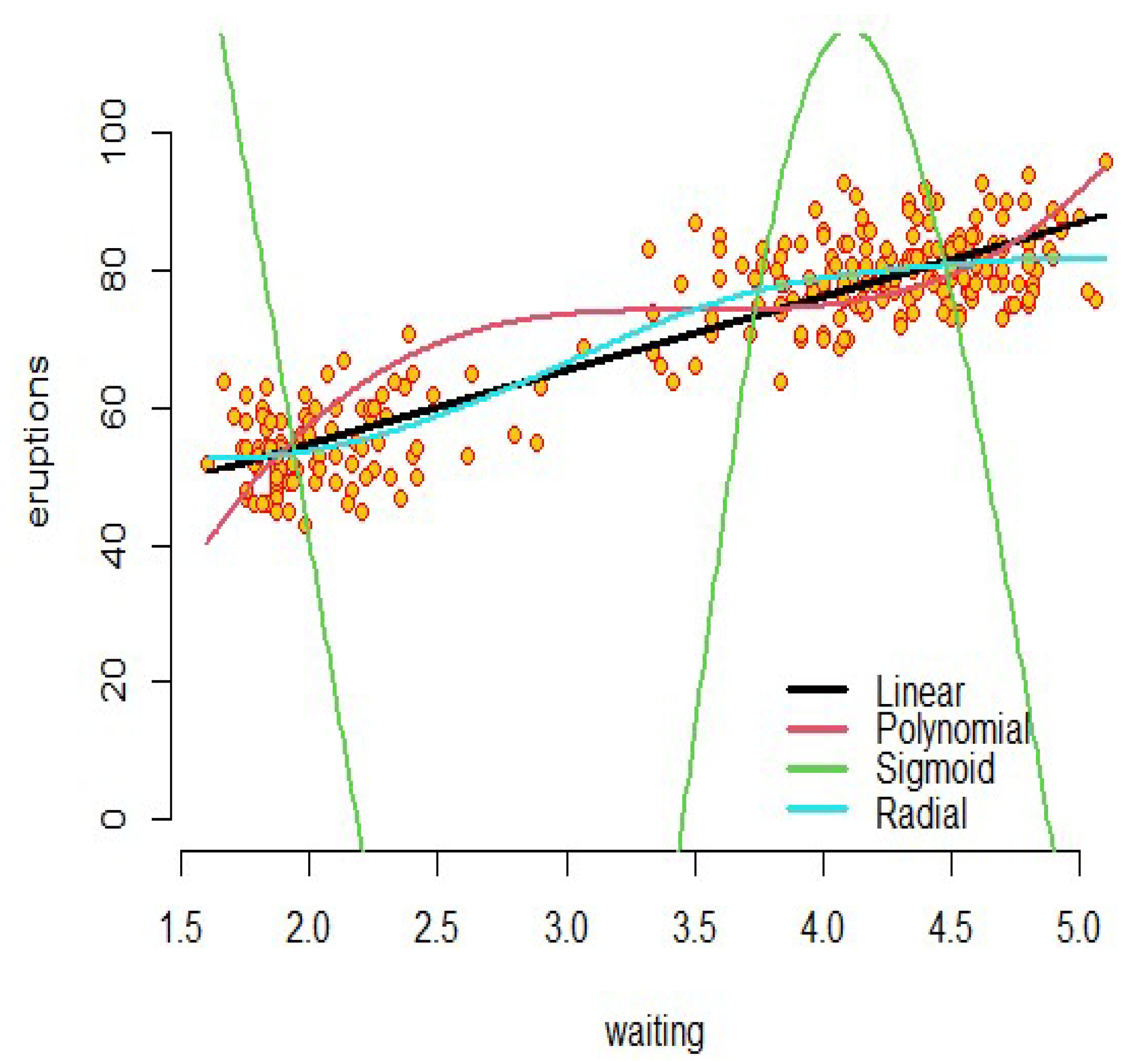
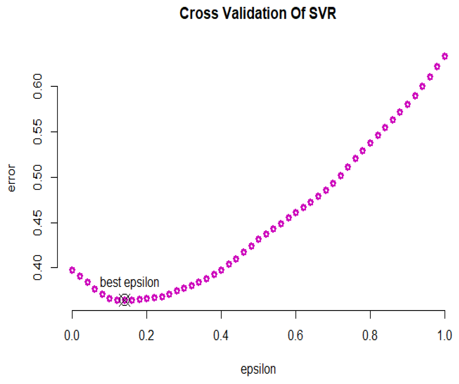
  • Example 2: As an interesting example, we can refer to real data (faithful) in R software. The dataset contains two variables: “eruptions” is the eruption time in minutes of the old faithful geyser, and is used as the response variable; and “waiting” is the waiting time between eruptions in minutes in Yellowstone National Park, Wyoming, USA as the predictor. The results of the support vector regression with introduced kernels are shown in Figure 2. For these fitted models, the sigmoid kernel has not performed well, but the other kernels have had acceptable results.

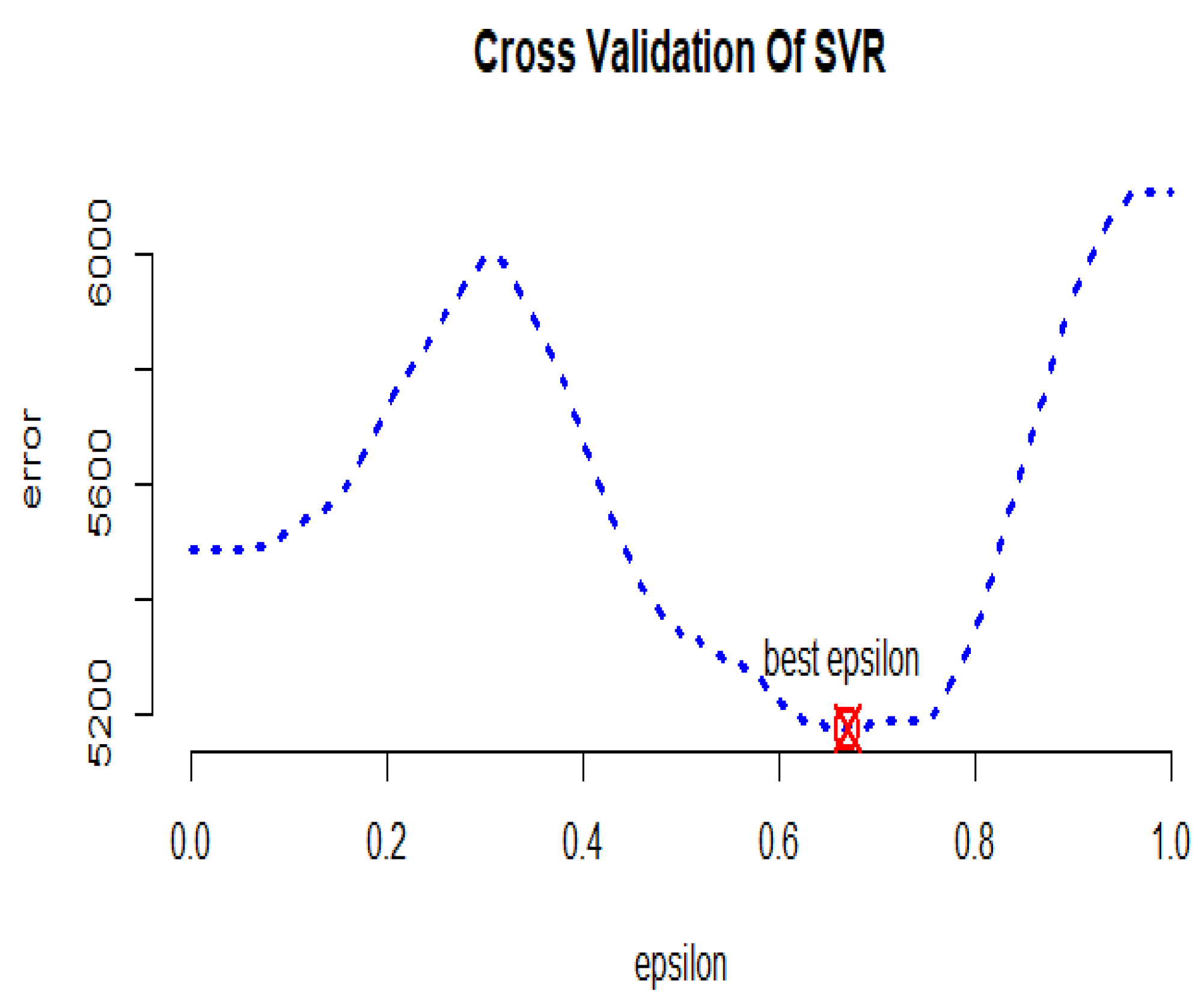
2.5.2. Generalized Support Vector Regression

As seen, the ridge, LASSO, and elastic net regression models are used by applying a penalty parameter subject to minimizing the complexity or to reducing the number of features selected in the final model. In the generalized support vector regression (GSVR) method, although the error fit may not be minimized, it can be flexible in order to make the final model more efficient. In this method, the optimal error is selected by minimizing the cross-validation criterion, which is defined as follows:
C . V . = 1 N k = 1 N y k f ^ ( k ) ( x , W ) 2 ,
where f ^ ( k ) ( x , W ) is the estimator obtained by omitting the k th observation ( x k , y k ) .
Furthermore, the error fit is defined as follows:
R = 1 2 W 2 + c i = 1 N | y i f ( x i , W ) | ϵ
where
| y f ( x , W ) | ϵ = 0 , | y f ( x , W ) | ϵ | y f ( x , W ) | ϵ , o . w .

3. Results Based on the Analysis of Real Datasets

3.1. Yeast Gene Data

In this section, the real high-dimensional data about the yeast genes are analyzed (http://www.exploredata.net/Downloads/Gene-Expression-Data-Set, accessed on 1 January 1997). This dataset of 4381 genes in 10 different ranges of time have been measured by Spellman. The information about genes are the explanatory variables and the times are considered as the response variable. More information about yeast gene data can be found in [25,26] that contain 4381 randomly selected genes as the predictor variables and a target variable denoting the cell cycle state as a response variable. The functional regression model for yeast gene data can be considered as follows:
Y i = j = 1 4381 X j ( t ) β j ( t ) + ϵ i , i = 1 , , 23 .
First, the explanatory variables are converted into the continuous curves using the spline basis function, which is depicted in Figure 3.
Using the principal component regression, we select the sufficient number of curves with a sufficient amount of data information (around 0.73 percent). Based on the scree diagram in Figure 4, it shows that five principal components are sufficient for describing these data.
According to Figure 5, we see that the amount of smoothness of converted variables is appropriate for these types of data.
According to Figure 5, we see that the amount of smoothness of the converted variables is appropriate for these types of data. The diagnostic plots of the functional principal component regression model depicted in Figure 6 identifies the goodness of fit. As it can be seen in this figure, the residuals do not follow a specific pattern, and the standardized residuals fall in the interval from 2 to 2, which is satisfactory for the functional principal component regression model.
The cross-validation plots of the LASSO and ridge regression models versus the penalty parameter are depicted in Figure 7 in order to obtain the optimal values of the penalty parameter, which are 1.62 and 845.10 , respectively.
The R-squared values for the functional principal component, LASSO, and ridge regression models are 0.9350 , 0.7778 , and 0.8079 , respectively. Now, the gene data are modeled using the SVR as follows:
Y i = w 0 + j = 1 4381 w j X j + ϵ i ,
where X j are the introduced genes, Y i are the times, and w i are the coefficients of the SVR model. Using the four proposed kernels, the modeling implements and the results are shown in Figure 8. As shown in this figure, the R-squared values for the linear, polynomial, radial, and sigmoid kernels are equal to 0.9657 , 0.7665 , 0.8363 , and 0.9442 , respectively. To compare the results intuitively, the straight line y = x is plotted in all of the diagrams of Figure 8. Therefore, according to these results, the linear and sigmoid kernels have performed better than the other kernels.
In Figure 9, the cross-validation criterion is used to obtain the optimal error value of the GSVR model, which is equal to 0.66 . Furthermore, the optimal values of parameters γ and c are equal to 0 and 0.01 , respectively.
Table 1 displays the summarized results and compares the fitted models based on the introduced criteria for the yeast gene data. According to the R-squared values, the SVR with the linear kernel, LASSO, and ridge have had satisfactory results. Based on the RMSE values, LASSO is more efficient than the other models. The SVR with linear and sigmoid kernels and the functional principal component regression have performed well based on the MAPE criterion. In general, the SVR model with the linear kernel has performed better than the other models.

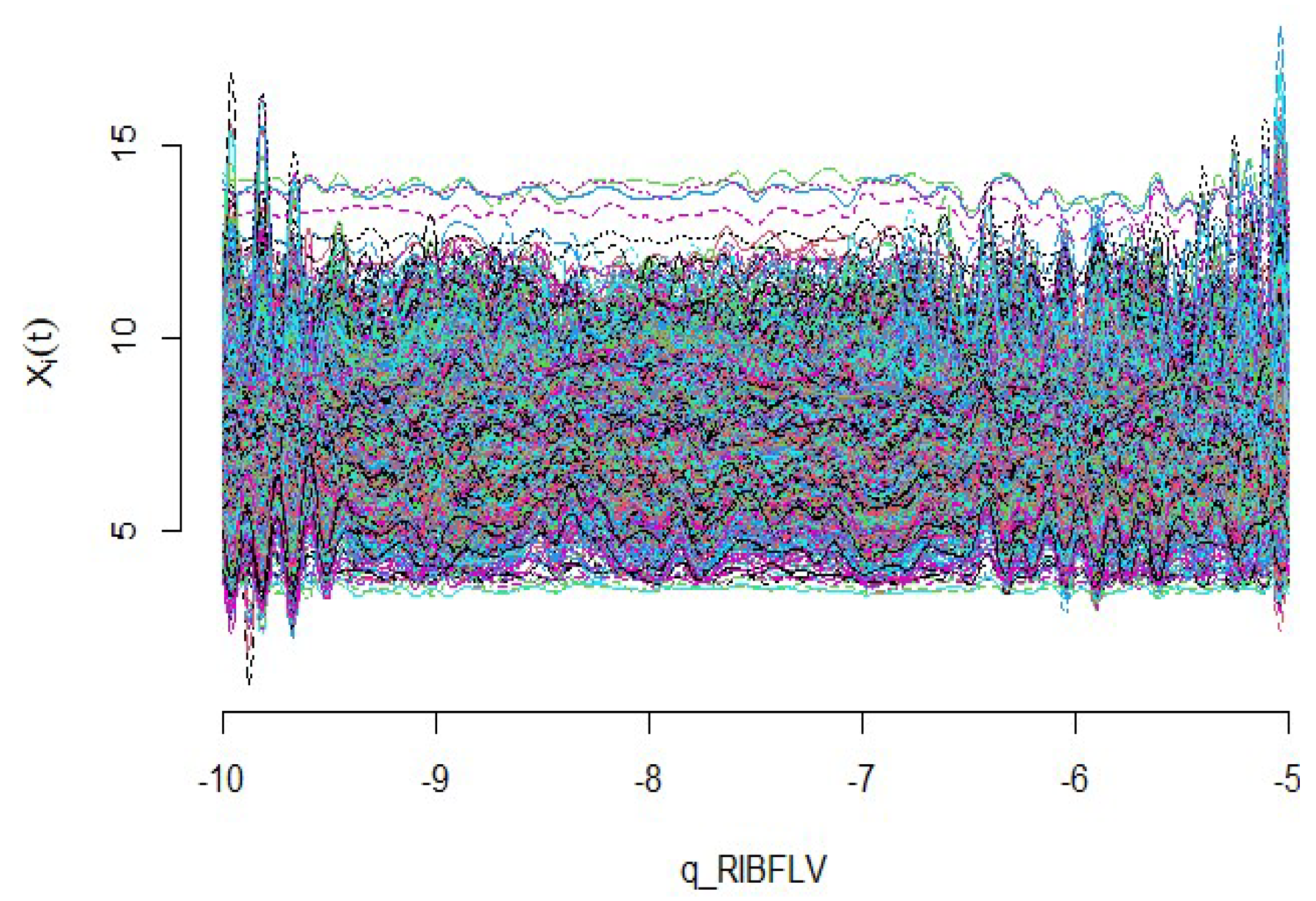
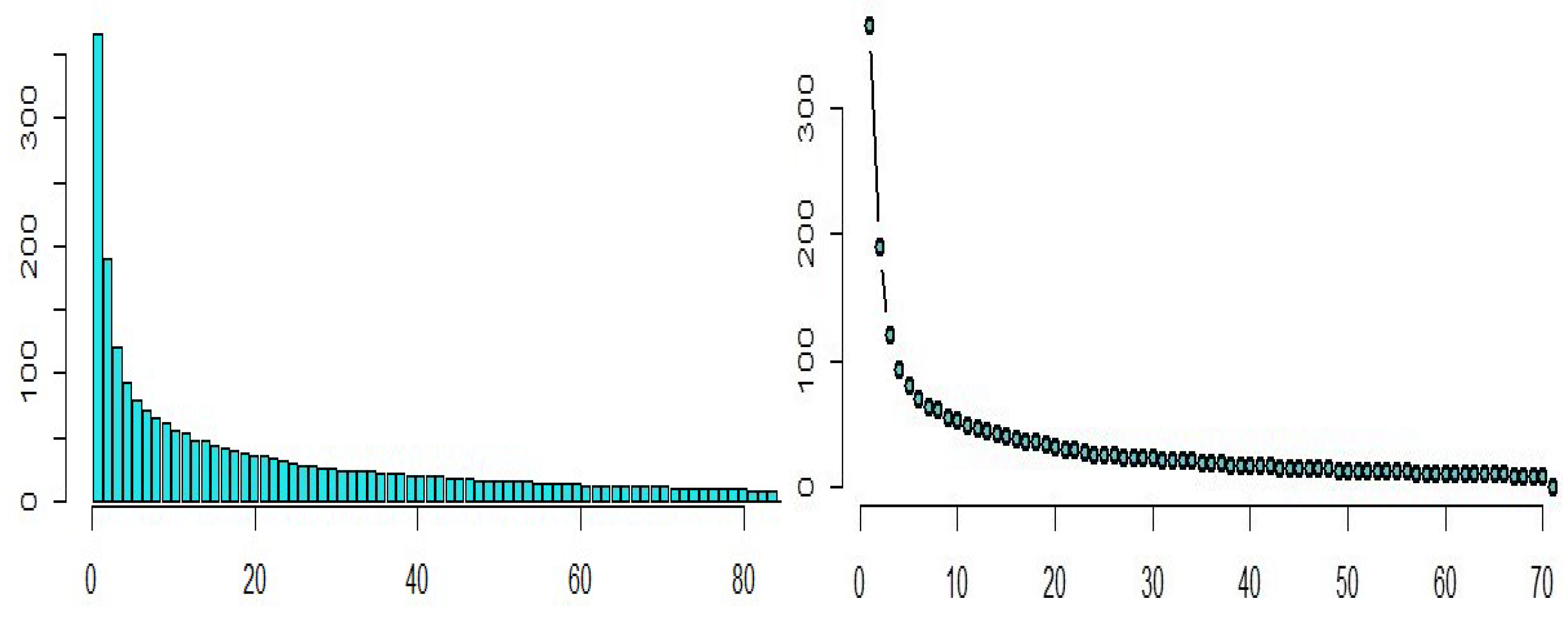
3.2. Riboflavin Data

To demonstrate the performance of the suggested techniques for the high-dimensional regression model, we analyze the riboflavin production dataset (also known as vitamin B2) in Bacillus subtilis, which can be found in the R package “hdi”. Riboflavin is one of the B vitamins that are water soluble. Riboflavin is naturally present in some foods, is added to some food products, and is available as a dietary supplement. This vitamin is an essential component of two major coenzymes, flavin mononucleotide (FMN; also known as riboflavin-5’-phosphate) and flavin adenine dinucleotide. In this dataset, based on n = 71 observations, there exists a single scalar response variable as the logarithm of the production rate of riboflavin and p = 4088 explanatory variables representing the logarithm of the expression level of 4088 gene surfaces. Foremost, the variables in the riboflavin data are converted into the continuous curves according to the number of optimized basic functions, and these can be observed in Figure 10. So, the functional regression model for these data can be considered as follows:
Y i = j = 1 4088 X j ( t ) β j ( t ) + ϵ i , i = 1 , , 71 ,
where Y i is the logarithm of the riboflavin production rate for the ith individual, X j ( t ) expresses the logarithm of the level of jth gene, and β j ( t ) is a functional coefficient of jth gene.
Based on the scree diagram in Figure 11, we see that 12 principal components are sufficient for describing these data, which have around 0.81 percent of information about the data.
According to Figure 12, we see that the amount of smoothness of the converted variables is appropriate for these types of data. To check the validity of the estimated model, we verify the diagnostic plots of the functional principal component regression model depicted in Figure 13. As it can be seen in this figure, the residuals do not follow a specific pattern and the standardized residuals fall in the standard interval; therefore, the functional principal component regression model is appropriate.
The cross-validation plots of the LASSO and ridge regression models are presented in Figure 14 in order to obtain the optimal values of the penalty parameters, which are 0.0335 and 6.2896 , respectively.
The R-squared values for the functional principal component, LASSO, and ridge regression are 0.6863 , 0.7617 , and 0.7848 , respectively. Now, the riboflavin production data are modeled using the SVR for different kernels, as follows:
Y i = w 0 + j = 1 4088 w j X j + ϵ i ,
where X j are the logarithm of gene surfaces, Y i are the logarithm of the riboflavin production rate, and w i are the coefficients of the SVR model. Using four proposed kernels, the modeling implements and the results are shown in Figure 15. To compare the results intuitively, the straight line y = x is plotted in all of the diagrams in this figure. As shown in Figure 15, the R-squared values for the linear, polynomial, radial, and sigmoid kernels are equal to 0.8319 , 0.3337 , 0.7461 , and 0.7345 , respectively. Therefore, according to these results, the linear kernel has performed better than the other kernels.
In Figure 16, the cross-validation criterion is used to obtain the optimal error value of the GSVR model, which is equal to 0.14 . Furthermore, the optimal values of parameters γ and c are equal to 1 and 10, respectively. Table 2 displays the summarized results and compares the fitted models based on the introduced criteria for the riboflavin production data. According to the R-squared values, the SVR with the sigmoid kernel and GSVR have had satisfactory results. Based on the RMSE values, the SVR with the linear kernel and GSVR are more efficient than the other models. The GSVR and SVR with the linear kernel have performed well based on the MAPE criterion. In general, the GSVR model has performed better than the other models.

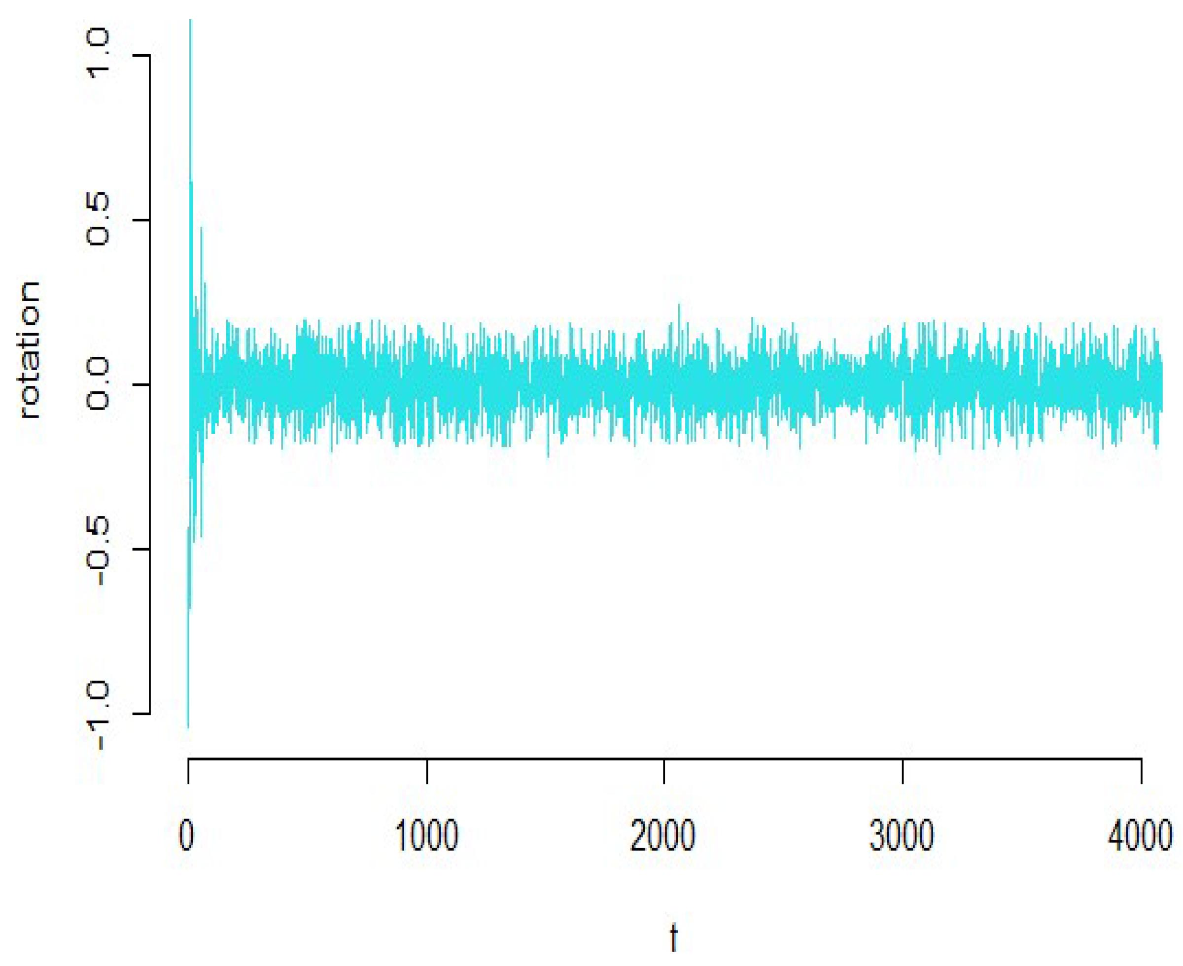
3.3. Simulated Dataset

Then, we performed some Monte Carlo simulation studies to examine the proposed models. Due to high-dimensional problem, as mentioned before, the number of explanatory variables should be greater than the number of observations ( p > n ) . Therefore, the explanatory variables with a dependent structure are simulated from the following model for n = 200 and p = 540 :
x i j = ( 1 ρ 2 ) 1 2 z i j + ρ z i p , i = 1 , , n , j = 1 , , p ,
where the random numbers z i j are the independent standard normal distribution, and ρ 2 determines the correlation between any two explanatory variables, which is equal to 0.9 in this research [27]. Hence, the response variable is obtained from the following formula:
y = X β + ϵ ,
where β i for i = 1 , , 0.4 p are generated from the standard normal distribution and β i = 0 for i > 0.4 p . Furthermore, the values of the errors ϵ i are generated randomly and independently from the normal distribution with zero mean and σ 2 = 1.44 . According to these types of data, firstly, the functional curves related to the explanatory variables are estimated. As seen in Figure 17, the simulated explanatory variables are converted into the continuous curves using the B-spline basic function.
Using the principal component regression analysis, we select the required number of curves with a sufficient amount of information about the data (around 0.70 percent), based on the scree diagram plotted in Figure 18, in which eight principal components can be found and are sufficient for describing these data.
According to Figure 19, we see that the amount of smoothness of the converted variables is appropriate for the simulated dataset. To check the validity of the estimated model, we turn to the diagnostic plots of the functional principal component regression model depicted in Figure 20. As it can be seen in this figure, the residuals do not follow a specific pattern, the standardized residuals fall in the standard interval; therefore, the functional principal component regression model is appropriate for the high-dimensional simulated data.
The cross-validation plots of the LASSO and ridge regression models are presented in Figure 21 to obtain the the optimal values of the penalty parameter.
The R-squared values for the functional principal component, LASSO, and ridge regression are obtained and they are 0.9738 , 0.9983 , and 0.9981 , respectively. Now, we will remodel the simulation data using the SVR for different kernels, as follows:
Y i = w 0 + j = 1 540 w j X j + ϵ i , i = 1 , , 200 ,
where w i are the coefficients of the SVR model. Using the four proposed kernels, the modeling implements and the results are shown in Figure 22. As shown in this figure, the R-squared values for the linear, polynomial, radial, and sigmoid kernels are equal to 0.9989 , 0.5901 , 0.2229 , and 0.9607 , respectively. Therefore, according to these results, the linear and radial kernels have had outstanding results rather than the other kernels.
In Figure 23, the cross-validation criterion is used to obtain the optimal error value of the GSVR model, which is equal to 0.36 . Furthermore, the optimal values of parameters γ and c are equal to 0.0 and 0.10 , respectively. Table 3 displays the summarized results and compares the fitted models based on the introduced criteria for the simulated dataset. According to the R-squared values, the SVR with the linear kernel and GSVR have had a satisfactory result. Based on the RMSE values, the GSVR is more efficient than the other models. The LASSO, ridge regression, SVR with linear kernel, and GSVR have performed well based on the MAPE criterion. Generally, the GSVR has performed better than the other models.
Moreover, we are reminded that modeling is completed and the figures are depicted using R software with e1071, fda.usc, glmnet, and hdi libraries.

4. Conclusions

The analysis of the high-dimensional data due to the non-invertibility of matrix X X is not possible with classical methods. Among the various modern methods and algorithms for solving the high-dimensional challenges, a support vector regression approach is a widely used and is a powerful technique in the field of machine learning, and can be a suitable choice for predicting high-dimensional datasets. In statistical modeling where the behavior of the data is a function of another variable, a functional data analysis is an essential tool. Therefore, in this research, some methods are the same as those for the functional principal components, LASSO, ridge, and support vector regression (with linear, polynomial, radial, and sigmoid kernels) and extended from the support vector regression (generalized support vector regression) using the cross-validation criterion, and were proposed to analyze and predict the high-dimensional datasets (yeast gene, riboflavin production, and simulated datasets). The numerical experiments showed that the generalized support vector regression and support vector regression with the linear kernel can be effectively applied to predict the high-dimensional datasets. As is known, obtaining the optimal value of the ridge parameter is not generally simple and it depends on the criterion used in the prediction problem and dataset. Furthermore, the ridge regression method combats the multicollinearity problem and estimates the parameters by adding shrinkage parameter k to the diagonal elements of X X , which leads to distortion of the data [28,29]. LASSO is based on balancing the opposing factors of bias and variance to build the most predictive model. In fact, LASSO shrinks the regression coefficients toward zero by penalizing the regression model with a l 1 -norm penalty term. In high-dimensional datasets, these properties may lead to shrink some coefficients of the effective predictors toward zero. This is the main drawback of LASSO. Another challenge in the LASSO method is the bias-variance trade-off in modeling which is related to the shrinkage parameter of the LASSO approach. Bias refers to how correct (or incorrect) the model is. A very simple model that makes a lot of mistakes is said to have a high bias. A very complicated model that performs well with its training data is said to have a low bias. Unfortunately, many of the suggestions made, for example that sample size (n) should be greater than 100 or that n should be greater than five times the number of variables, are based on minimal empirical evidence, which is a drawback of the principal component regression method. Furthermore, the reduction in dimensionality that can often be achieved through a principal components analysis is possible only if the original variables are correlated; if the original variables are independent of one another, a principal components analysis cannot lead to any simplification. To combat these drawbacks, as new research for the future, we suggest to improve the support vector regression method using penalized mixed-integer non-linear programming that can be solved using metaheuristic algorithms.

Author Contributions

Conceptualization, M.R. and A.R.; methodology, M.R.; software, A.R. and F.J.; validation, N.A.M. and M.R.; formal analysis, A.R. and F.J.; investigation, N.A.M. and M.R.; resources, A.R.; data curation, A.R.; writing—original draft preparation, M.R. and A.R.; writing—review and editing, N.A.M. and M.R.; visualization, A.R. and F.J.; supervision, M.R.; project administration, M.R. and N.A.M.; funding acquisition, N.A.M. and M.R. All authors have read and agreed to the published version of the manuscript.

Funding

This research was funded by Universiti Malaya Research Grant (GPF083B–2020).

Data Availability Statement

All used datasets are available in R software at “e1071”, “fda.usc”, and “hdi libraries”.

Acknowledgments

We would like to sincerely thank two anonymous reviewers for their constructive comments, which led us to put many details in the paper and improve the presentation.

Conflicts of Interest

The authors declare no conflict of interest.

References

  1. Taavoni, M.; Arashi, M. High-dimensional generalized semiparametric model for longitudinal data. Statistics 2021, 55, 831–850. [Google Scholar] [CrossRef]
  2. Efron, B.; Hastie, T. Computer Age Statistical Inference; Cambridge University Press: Cambridge, UK, 2016. [Google Scholar]
  3. Jolliffe, I.T. Principal Component Analysis; Springer: Aberdeen, UK, 2002. [Google Scholar]
  4. Tibshirani, R. Regression Shrinkage and Selection via the Lasso. J. R. Stat. Soc. Ser. B 1996, 58, 267–288. [Google Scholar] [CrossRef]
  5. Hoerl, A.E.; Kennard, R.W. Ridge regression: Some simulation. Commun. Stat. 1975, 4, 105–123. [Google Scholar] [CrossRef]
  6. Vapni, V.N. The Nature of Statistical Learning Theory; Springer: New York, NY, USA, 1995. [Google Scholar]
  7. Kao, L.J.; Chiu, C.C.; Lu, C.J.; Yang, J.L. Integration of nonlinear independent component analysis and support vector regression for stock price forecasting. Neurocomputing 2013, 99, 534–542. [Google Scholar] [CrossRef]
  8. Xiao, Y.; Xiao, J.; Lu, F.; Wang, S. Ensemble anns-pso-ga approach for day-ahead stock e-exchange prices forecasting. Int. J. Comput. Intell. Syst. 2014, 7, 272–290. [Google Scholar] [CrossRef] [Green Version]
  9. Ramsay, J.O.; Silverman, B.W. Functional Data Analysis; Springer: New York, NY, USA, 2005. [Google Scholar]
  10. Ferraty, F.; Vieu, P. Nonparametric Functional Data Analysis: Theory and Practice; Springer: New York, NY, USA, 2006. [Google Scholar]
  11. Goldsmith, J.; Scheipl, F. Estimator selection and combination in scalar-on-function regression. Comput. Stat. Data Anal. 2014, 70, 362–372. [Google Scholar] [CrossRef]
  12. Choudhury, S.; Ghosh, S.; Bhattacharya, A.; Fernandes, K.J.; Tiwari, M.K. A real time clustering and SVM based price-volatility prediction for optimal trading strategy. Neurocomputing 2014, 131, 419–426. [Google Scholar] [CrossRef]
  13. Nayak, R.K.; Mishra, D.; Rath, A.K. A naïve svm-knn based stock market trend reversal analysis for indian benchmark indices. Appl. Soft Comput. 2015, 35, 670–680. [Google Scholar] [CrossRef]
  14. Patel, J.; Shah, S.; Thakkar, P.; Kotecha, K. Predicting stock market index using fusion of machine learning techniques. Expert Syst. Appl. 2015, 42, 2162–2172. [Google Scholar] [CrossRef]
  15. Araújo, R.D.A.; Oliveira, A.L.; Meira, S. A hybrid model for high-frequency stock market forecasting. Expert Syst. Appl. 2015, 42, 4081–4096. [Google Scholar] [CrossRef]
  16. Sheather, S. A Modern Approach to Regression with R; Springer: New York, NY, USA, 2009. [Google Scholar]
  17. Roozbeh, M.; Babaie–Kafaki, S.; Manavi, M. A heuristic algorithm to combat outliers and multicollinearity in regression model analysis. Iran. J. Numer. Anal. Optim. 2022, 12, 173–186. [Google Scholar]
  18. Arashi, M.; Golam Kibria, B.M.; Valizadeh, T. On ridge parameter estimators under stochastic subspace hypothesis. J. Stat. Comput. Simul. 2017, 87, 966–983. [Google Scholar] [CrossRef]
  19. Fallah, R.; Arashi, M.; Tabatabaey, S.M.M. On the ridge regression estimator with sub-space restriction. Commun. Stat. Theory Methods 2017, 46, 11854–11865. [Google Scholar] [CrossRef]
  20. Roozbeh, M. Optimal QR-based estimation in partially linear regression models with correlated errors using GCV criterion. Comput. Stat. Data Anal. 2018, 117, 45–61. [Google Scholar] [CrossRef]
  21. Roozbeh, M.; Najarian, M. Efficiency of the QR class estimator in semiparametric regression models to combat multicollinearity. J. Stat. Comput. Simul. 2018, 88, 1804–1825. [Google Scholar] [CrossRef]
  22. Yüzbaşi, B.; Arashi, M.; Akdeniz, F. Penalized regression via the restricted bridge estimator. Soft Comput. 2021, 25, 8401–8416. [Google Scholar] [CrossRef]
  23. Zhang, X.; Xue, W.; Wang, Q. Covariate balancing functional propensity score for functional treatments in cross-sectional observational studies. Comput. Stat. Data Anal. 2021, 163, 107303. [Google Scholar] [CrossRef]
  24. Miao, R.; Zhang, X.; Wong, R.K. A Wavelet-Based Independence Test for Functional Data with an Application to MEG Functional Connectivity. J. Am. Stat. Assoc. 2022, 1–14. [Google Scholar] [CrossRef]
  25. Spellman, P.T.; Sherlock, G.; Zhang, M.Q.; Iyer, V.R.; Anders, K.; Eisen, M.B.; Brown, P.O.; Botstein, D.; Futcher, B. Comprehensive Identification of Cell Cycle–regulated Genes of the Yeast Saccharomyces cerevisiae by Microarray Hybridization. Mol. Biol. Cell 1998, 9, 3273–3297. [Google Scholar] [CrossRef]
  26. Carlson, M.; Zhang, B.; Fang, Z.; Mischel, P.; Horvath, S.; Nelson, S.F. Gene Connectivity. Function, and Sequence Conservation: Predictions from Modular Yeast Co-expression Networks. BMC Genom. 2006, 7, 40. [Google Scholar] [CrossRef] [PubMed]
  27. McDonald, G.C.; Galarneau, D.I. A Monte Carlo evaluation of some ridge-type estimators. J. Am. Stat. Assoc. 1975, 70, 407–416. [Google Scholar] [CrossRef]
  28. Roozbeh, M.; Babaie–Kafaki, S.; Aminifard, Z. Two penalized mixed–integer nonlinear programming approaches to tackle multicollinearity and outliers effects in linear regression model. J. Ind. Manag. Optim. 2020, 17, 3475–3491. [Google Scholar] [CrossRef]
  29. Roozbeh, M.; Babaie–Kafaki, S.; Aminifard, Z. Improved high-dimensional regression models with matrix approximations applied to the comparative case studies with support vector machines. Optim. Methods Softw. 2022, 37, 1912–1929. [Google Scholar] [CrossRef]
Figure 1. SVR model for the simulated data.
Symmetry 15 01262 g001
Figure 2. SVR model for the faithful data.
Symmetry 15 01262 g002
Figure 3. Yeast gene data curves.
Symmetry 15 01262 g003
Figure 4. Scree diagram for the yeast gene data.
Symmetry 15 01262 g004
Figure 5. Diagram of the functional coefficients of the yeast gene data.
Symmetry 15 01262 g005
Figure 6. Diagnostic plots for the functional principal component regression model for the yeast gene data.
Symmetry 15 01262 g006
Figure 7. Penalty cross-validation diagram for the yeast gene data.
Symmetry 15 01262 g007
Figure 8. The diagram of the real values versus the fitted values for the SVR of the yeast gene data.
Symmetry 15 01262 g008
Figure 9. GSVR cross-validation diagram for the yeast gene data.
Symmetry 15 01262 g009
Figure 10. Riboflavin production data curves.
Symmetry 15 01262 g010
Figure 11. Scree diagram for the riboflavin production data.
Symmetry 15 01262 g011
Figure 12. Diagram of the functional coefficients for the riboflavin production data.
Symmetry 15 01262 g012
Figure 13. Diagnostic plots for the functional principal component regression model for the riboflavin production data.
Symmetry 15 01262 g013
Figure 14. Penalty cross-validation diagram for the riboflavin production data.
Symmetry 15 01262 g014
Figure 15. The diagram of the real values versus the fitted values for the SVR of the riboflavin production data.
Symmetry 15 01262 g015
Figure 16. GSVR cross-validation diagram for the riboflavin production data.
Symmetry 15 01262 g016
Figure 17. Simulated data curves.
Symmetry 15 01262 g017
Figure 18. Scree diagram of the simulated data.
Symmetry 15 01262 g018
Figure 19. Estimation of the functional coefficients of the simulated data.
Symmetry 15 01262 g019
Figure 20. Diagnostic plots for the functional principal component regression model of the simulated data.
Symmetry 15 01262 g020
Figure 21. Penalty cross-validation for the simulated data.
Symmetry 15 01262 g021
Figure 22. The diagram of the real values versus the fitted values for the SVR of the simulated dataset.
Symmetry 15 01262 g022
Figure 23. GSVR cross-validation diagram for the simulated dataset.
Symmetry 15 01262 g023
Table 1. Comparison of the proposed approaches for the yeast gene data.
CriterionR 2 RMSEMAPE
Method
Functional principal component 0.9350 22.1786 0.1569
Ridge regression 0.9526 27.2272 0.2551
LASSO regression 0.9584 18.8379 0.2194
SVR with linear kernel 0.9657 23.1250 0.1428
SVR with polynomial kernel 0.7665 50.0320 0.2920
SVR with sigmoid kernel 0.9442 29.8033 0.1583
SVR with radial kernel 0.8363 45.0107 0.2702
GSVR 0.9178 22.8142 0.1614
Table 2. Comparison of the proposed approaches for the riboflavin production data.
CriterionR 2 RMSEMAPE
Method
Functional principal component 0.6863 0.4238 0.0535
Ridge regression 0.7848 0.4025 0.0498
LASSO regression 0.7617 0.5365 0.0733
SVR with linear kernel 0.8319 0.3056 0.0352
SVR with polynomial kernel 0.3337 0.7170 0.0854
SVR with sigmoid kernel 0.9442 29.8033 0.1583
SVR with radial kernel 0.7461 0.6217 0.0754
GSVR 0.8363 0.3071 0.0339
Table 3. Comparison of the proposed approaches for the the simulation data.
CriterionR 2 RMSEMAPE
Method
Functional principal component 0.9738 82.4995 0.0015
Ridge regression 0.9981 8.0627 0.0001
LASSO regression 0.9983 7.6356 0.0001
SVR with linear kernel 0.9989 7.8584 0.0001
SVR with polynomial kernel 0.5901 237.1014 0.0024
SVR with sigmoid kernel 0.2229 1102.886 0.0186
SVR with radial kernel 0.9607 39.6032 0.0003
GSVR 0.9984 6.4692 0.0001
Disclaimer/Publisher’s Note: The statements, opinions and data contained in all publications are solely those of the individual author(s) and contributor(s) and not of MDPI and/or the editor(s). MDPI and/or the editor(s) disclaim responsibility for any injury to people or property resulting from any ideas, methods, instructions or products referred to in the content.

